Search for $ZH\rightarrow\ell^{+}\ell^{-}b\bar{b}$ production in $9.7$ fb^-1 of $p\bar{p}$ collisions with the D0 detector

Abstract

We present a search for the standard model (SM) Higgs boson produced in association with a $Z$ boson in 9.7 fb^-1 of $p\bar{p}$ collisions collected with the D0 detector at the Fermilab Tevatron Collider at $\sqrt{s}$ = 1.96 $\mathrm{Te\kern-1.00006ptV}$. Selected events contain one reconstructed $Z\rightarrow e^{+}e^{-}$ or $Z\rightarrow\mu^{+}\mu^{-}$ candidate and at least two jets, including at least one jet likely to contain a $b$ quark. To validate the search procedure, we also measure the cross section for $ZZ$ production, and find that it is consistent with the SM expectation. We set upper limits at the $95\%$ C.L. on the product of the $ZH$ production cross section and branching ratio $\mathcal{B}(H\to\mbox{$b\overline{b}$})$ for Higgs boson masses $90\leq M_{H}\leq 150~{}\mathrm{Ge\kern-1.00006ptV}$. The observed (expected) limit for $M_{H}=125~{}\mathrm{Ge\kern-1.00006ptV}$ is a factor of 7.1 (5.1) larger than the SM prediction.

I Introduction

In the standard model (SM), the spontaneous breaking of the electroweak gauge symmetry generates masses for the $W$ and $Z$ bosons and produces a new scalar elementary particle, the Higgs boson higgs . Precision electroweak data, including the latest $W$ boson mass measurements from the CDF cdf-wmass and D0 d0-wmass collaborations and the latest Tevatron combination for the top quark mass tev-top , constrain the mass of the SM Higgs boson to $M_{H}<$ 152 GeV ew-fit at the 95% confidence level (C.L.). Direct searches at the CERN $e^{+}e^{-}$ Collider (LEP) lep-higgs , by the CDF and D0 collaborations at the Fermilab Tevatron $p\overline{p}$ Collider tev-results , and by the ATLAS and CMS collaborations at the CERN Large Hadron Collider (LHC) atlas-results ; cms-results further restrict the allowed range to $122.1<M_{H}<127.0$ GeV. ATLAS and CMS have discovered a new boson with properties consistent with those of the SM Higgs boson at ${M_{H}~{}\approx~{}126~{}\mathrm{Ge\kern-1.00006ptV}}$ new-atlas-results ; new-cms-results , primarily through its decays into $\gamma\gamma$ and $ZZ$, while the CDF and D0 collaborations have reported combined evidence for a particle consistent with such a boson produced in association with weak bosons and decaying to $b\bar{b}$ tev-results2 .

For ${M_{H}\lesssim 135~{}\mathrm{Ge\kern-1.00006ptV}}$, the dominant Higgs boson decay is to the $b\bar{b}$ final state. At the Tevatron the best sensitivity to a low mass Higgs boson is obtained from the analysis of its production in association with a $W$ or $Z$ boson and its subsequent decay into pairs of $b$ quarks. Evidence for a signal in this decay mode complements the ATLAS and CMS observations and provides further indication that the new particle is consistent with the SM Higgs boson that also couples directly to fermions.

We present a search for the process $ZH\rightarrow\ell^{+}\ell^{-}b\bar{b}$, where $\ell$ is either a muon or an electron, in $9.7$ fb^-1 of $p\bar{p}$ collisions at $\sqrt{s}$ = 1.96 $\mathrm{Te\kern-1.00006ptV}$ using the D0 detector. This Article is a detailed description of a published Letter zh_prl providing inputs included in the CDF and D0 combination described in Ref. tev-results2 . The CDF collaboration has performed a search in the same final state cdf-zhiggs . This analysis extends and supersedes the previous D0 result obtained on 4.2 fb^-1 of integrated luminosity pubzh .

We select events that contain a $Z$ boson candidate, reconstructed in one of four independent channels defined by lepton identification criteria. Selected events must also contain a Higgs boson candidate, reconstructed from two jets. At least one jet must be identified as likely to originate from a $b$ quark (“$b$ tagged”). The backgrounds to this selection include the production of a $Z$ boson in association with jets, $t\overline{t}$ production, diboson production, and multijet events with non-prompt muons or electrons, or with jets misidentified as electrons. They are estimated using Monte Carlo (MC) simulations and control samples in the data. We employ a kinematic fit to improve the reconstruction of the $H\to\mbox{$b\overline{b}$}$ resonance. Subsequently, we develop a two-stage multivariate analysis to separate the signal from the backgrounds and extract results from the shapes of the resulting multivariate discriminants. To validate the search procedure, we also present a measurement of the $ZZ$ production cross section in the same final state used for the Higgs boson search.

We describe the D0 detector in Section II and the event selection in the four analysis channels in Section III. Background and signal MC simulations are detailed in Section IV and multijet estimation is described in Section V. In Section VI we discuss the normalization applied to the background samples. The kinematic fit is described in Section VII. We describe the multivariate analysis strategy in Section VIII and the systematic uncertainties affecting the final results in Section IX. We present the results for Higgs boson production and diboson production in Section X and summarize our results in Section XI.

II The D0 detector

The D0 detector d0det ; run1det consists of a central tracking system in a 2 T superconducting solenoidal magnet, surrounded by a central preshower (CPS) detector, a liquid–argon sampling calorimeter, and a muon spectrometer. The central tracking system consists of a silicon microstrip tracker (SMT) and a scintillating fiber tracker (CFT), and provides coverage for charged particles in the pseudorapidity d0coords range $|\mbox{$\eta_{\mathrm{det}}$}|<3$, where $\eta_{\mathrm{det}}$ is the pseudorapidity measured with respect to the center of the detector. The CPS is located immediately before the inner layer of the calorimeter, and has about one radiation length of absorber, followed by three layers of scintillating strips. The calorimeter consists of a central cryostat (CC), covering $|\mbox{$\eta_{\mathrm{det}}$}|<1.1$, and two end cryostats (EC), covering up to $|\mbox{$\eta_{\mathrm{det}}$}|\approx 4.2$. In each cryostat the calorimeters are divided into electromagnetic (EM) layers on the inside and hadronic layers on the outside. Plastic scintillator detectors improve the calorimeter measurement in the inter-cryostat regions (ICRs, $1.1<|\mbox{$\eta_{\mathrm{det}}$}|<1.5$) between the CC and the ECs. The muon spectrometer is located beyond the calorimeter and consists of a layer of tracking detectors and scintillation trigger counters before a 1.8 T iron toroidal magnet, followed by two similar layers after the toroid. It provides coverage up to $|\mbox{$\eta_{\mathrm{det}}$}|\approx 2$. The instantaneous luminosity is measured by a system composed of two disks of scintillators positioned in front of the ECs. A three-level trigger system selects events for data logging and subsequent offline analysis.

III Event Selection

The search is performed in four independent channels defined by the subdetectors used for lepton identification: the dimuon channel ($\mu\mu$), the muon + isolated track channel ($\mu\mu_{\rm trk}$), the dielectron channel ($ee$), and the electron + ICR electron channel ($ee_{\rm ICR}$). The data for this analysis were collected from April 2002 to February 2006 (Run $2$a), and from June 2006 to September 2011 (Run $2$b). Between Run $2$a and Run $2$b, a new layer of the SMT was installed and the trigger system was upgraded d0upgrade . Run $2$a corresponds to an integrated luminosity of 1.1 fb^-1. Run $2$b is further sub-divided into three periods that we analyze independently to account for time-dependent effects in the performance of the detector. We refer to them as Runs 2b1 (corresponding to an integrated luminosity of 1.2 fb^-1), 2b2 (3.0 fb^-1), and 2b3 (4.4 fb^-1).

III.1 Triggering

In the $ee$ and $ee_{\rm ICR}$ channels we analyze events acquired predominantly with triggers that provide real-time identification of electrons and jets. In the $ee$ channel we accept events that satisfy any trigger requirement, with a measured efficiency consistent with 100% within 1%. In the $ee_{\rm ICR}$ channel the set of triggers used has an efficiency of 90–100% depending on the region of the detector toward which the electron points, and we apply the trigger efficiency, measured in data and parametrized by electron $\eta$, electron $\phi$, and jet transverse momentum, to the MC events as a weight. Specific selection requirements applied to the two channels are described in Sec. III.2.

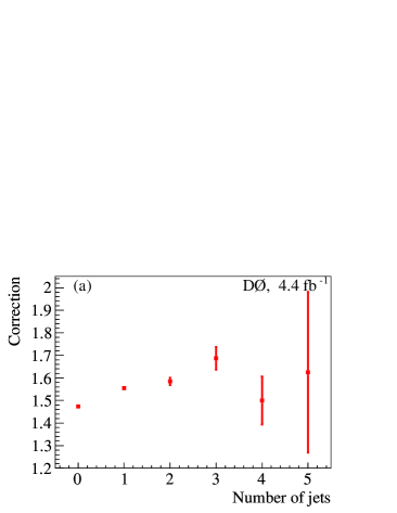
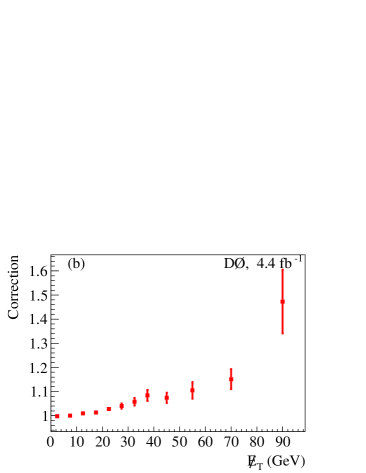
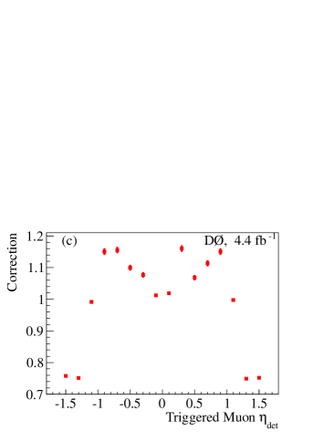
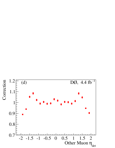
In the $\mu\mu$ and $\mu\mu_{\rm trk}$ channels we accept events that satisfy any trigger requirement, although most were recorded using triggers that contain muon selection terms. To correctly model the efficiency of the inclusive set of triggers for these events, we develop a correction based on a reference data sample, for which we demand that the leading muon with $|\mbox{$\eta_{\mathrm{det}}$}|<1.5$ satisfies one of the triggers that require a single muon. We confirm that this reference sample is well modeled by the MC when we apply the corresponding trigger efficiencies. We then derive a normalization correction factor equal to the ratio of the number of events in the inclusively triggered sample to the single-muon trigger sample in bins of the number of jets in the event. Shape-only correction factors are determined in zero-jet events in bins of $\eta$ of each of the two muons and the transverse energy imbalance ($\not{E}_{\rm T}$). To account for changes in the trigger conditions, and hence efficiency, with time, we derive separate corrections for each of the four data-taking periods. Figure 1 shows as an example the correction factors for the $\mu\mu$ channel in Run $2$b3.

After imposing data quality requirements, the integrated luminosity recorded by these triggers is 9.7 fb^-1 in each channel.

Figure 1: (color online). Trigger correction factors for the $\mu\mu$ channel in Run $2$b3 as a function of (a) jet multiplicity, (b) $\not{E}_{\rm T}$, (c) $\eta_{\mathrm{det}}$ of the triggered muon, and (d) $\eta_{\mathrm{det}}$ of the other muon. The correction applied to the single muon trigger is the product of all four components.

III.2 Offline Event Selection

The event selection in all channels requires a $p\overline{p}$ interaction vertex (PV) that has at least three associated tracks, and is located within $\pm$60 cm of the center of the detector along the beam direction. In the dimuon channel ($\mu\mu$) we select events with at least two muons identified in the muon system, matched to central tracks with transverse momenta $\mbox{$p_{\rm T}$}>10~{}\mathrm{Ge\kern-1.00006ptV}$ and $|\mbox{$\eta_{\mathrm{det}}$}|~{}<~{}2$. At least one muon must have $|\mbox{$\eta_{\mathrm{det}}$}|~{}<~{}1.5$ and $\mbox{$p_{\rm T}$}>15~{}\mathrm{Ge\kern-1.00006ptV}$. The two muons must also have opposite charges. The distance between the PV and each of the muon tracks along the $z$ axis, $d_{\mathrm{PV}}^{z}$, must be less than 1 cm. The distance of closest approach of each muon track to the PV in the plane transverse to the beam direction, $d_{\mathrm{PV}}$, must be less than $0.04~{}$cm for tracks with at least one hit in the SMT. Muon tracks without any SMT hits must have $d_{\mathrm{PV}}~{}<~{}0.2$ cm, and the momentum resolution of these tracks is improved through a constraint to the position of the PV in the transverse plane.

At least one muon must be separated from all jets (see below) by $\Delta\mathcal{R}~{}=~{}\sqrt{(\Delta\eta)^{2}+(\Delta\phi)^{2}}>0.5$, where the jets must have $\mbox{$p_{\rm T}$}~{}>~{}20~{}\mathrm{Ge\kern-1.00006ptV}$ and $|\mbox{$\eta_{\mathrm{det}}$}|~{}<~{}2.5$. If only one muon satisfies this criterion, we also require that the ratio ($R_{\mathrm{TRK}}$) of the vector sum of the transverse momenta of all tracks in a cone of $\Delta\mathcal{R}~{}<~{}0.5$ around that muon to its $p_{\rm T}$ satisfy $R_{\mathrm{TRK}}~{}<~{}0.2$, and that the ratio ($R_{\mathrm{CAL}}$) of the transverse energy deposited in the calorimeter in a hollow cone with $0.1~{}<~{}\Delta\mathcal{R}~{}<~{}0.4$ around that muon to its $p_{\rm T}$ satisfy $R_{\mathrm{CAL}}~{}<~{}0.2$. If both muons are separated from jets, then only the leading muon must satisfy the additional track and calorimeter isolation requirements described above. To reduce contamination from cosmic rays, the muon tracks must not be back-to-back in $\eta$ and $\phi$.

The $\mu\mu_{\rm trk}$ channel is designed to recover dimuon events in which one muon is not identified in the muon system, primarily because of gaps in the muon system coverage. In this channel we require the presence of exactly one muon with $|\mbox{$\eta_{\mathrm{det}}$}|~{}<~{}1.5$ and $\mbox{$p_{\rm T}$}~{}>~{}15~{}\mathrm{Ge\kern-1.00006ptV}$ that must satisfy the same tracker and calorimeter isolation requirements used for the $\mu\mu$ channel. We also require the presence of an isolated track with $|\mbox{$\eta_{\mathrm{det}}$}|<2$ and $\mbox{$p_{\rm T}$}>20~{}\mathrm{Ge\kern-1.00006ptV}$, separated from the muon by $\Delta\mathcal{R}~{}>~{}0.1$. This track-only muon ($\mu_{\rm trk}$) must have at least one SMT hit, $d_{\mathrm{PV}}<0.02$ cm, and $d_{\mathrm{PV}}^{z}<1$ cm. It must be separated from all jets having $\mbox{$p_{\rm T}$}~{}>15~{}\mathrm{Ge\kern-1.00006ptV}$ and $|\mbox{$\eta_{\mathrm{det}}$}|<2.5$ by $\Delta\mathcal{R}~{}>~{}0.5$. It must also satisfy the same tracker and calorimeter isolation requirements as the first muon. The muons must have opposite charges. To ensure that the $\mu\mu$ and $\mu\mu_{\rm trk}$ selections do not overlap, we reject events that contain any additional muons with $|\mbox{$\eta_{\mathrm{det}}$}|~{}<~{}2$ and $\mbox{$p_{\rm T}$}~{}>10~{}\mathrm{Ge\kern-1.00006ptV}$. For the small fraction of events (approximately 0.1%) with more than one track passing these requirements, the track whose invariant mass with the muon is closest to the $Z$ boson mass is chosen.

In the dielectron ($ee$) channel we select events with at least two electrons with $\mbox{$p_{\rm T}$}~{}>~{}15~{}\mathrm{Ge\kern-1.00006ptV}$ that pass selection requirements based on the energy deposition and shower shape in the calorimeter and the CPS. Electrons are accepted in the CC with $|\mbox{$\eta_{\mathrm{det}}$}|<1.1$ and in the EC with $1.5<|\mbox{$\eta_{\mathrm{det}}$}|<2.5$, but at least one of the electrons must be identified in the CC. Electrons are selected from EM clusters reconstructed within a cone of radius $\mathcal{R}~{}=~{}0.2$ and satisfying the following requirements: (i) at least 90% (97%) of the cluster energy is deposited in the EM calorimeter of the CC (EC); (ii) the calorimeter isolation variable $I=[E_{\mathrm{tot}}^{0.4}-E_{\mathrm{EM}}^{0.2}]/E_{\mathrm{EM}}^{0.2}$ is less than 0.09 (0.05) in the CC (EC), where $E_{\mathrm{tot}}^{0.4}$ is the total energy in a cone of radius $\mathcal{R}~{}=~{}0.4$ and $E_{\mathrm{EM}}^{0.2}$ is the EM energy in a cone of radius $\mathcal{R}~{}=~{}0.2$; (iii) the scalar sum of the transverse momenta of all tracks in a hollow cone of $0.05<\Delta\mathcal{R}<0.4$ around the electron is less than 4 $\mathrm{Ge\kern-1.00006ptV}$ in the CC, and less than or equal to $0$ to $2$ $\mathrm{Ge\kern-1.00006ptV}$ in the EC, depending on $\eta_{\mathrm{det}}$ of the electron; (iv) the output of an artificial neural network – which combines the energy deposition in the first EM layer, track isolation, and energy deposition in the CPS – is consistent with that expected from an electron; (v) CC electrons must match central tracks or a set of hits in the tracker consistent with that of an electron trajectory; and (vi) for EC electrons the energy-weighted cluster width in the third EM layer must be consistent with that expected from an EM shower.

In the $ee_{\rm ICR}$ channel, events must contain exactly one electron in either the CC or EC with $\mbox{$p_{\rm T}$}>15~{}\mathrm{Ge\kern-1.00006ptV}$, and a track pointing toward one of the ICRs, where electromagnetic object identification is compromised. This ICR track must be matched to a calorimeter energy deposit with $E_{\mathrm{T}}>15~{}\mathrm{Ge\kern-1.00006ptV}$. The ICR electron must satisfy a requirement on the output of a neural network, designed to separate electrons from jets, that combines the track quality, the track isolation and the energy deposition in the scintillator detectors located in the ICR. If the electron is found in the EC, we require that the ICR electron has the same rapidity sign. In both the $ee$ and the $ee_{\rm ICR}$ channels, any tracks matched to electrons must have $d_{\mathrm{PV}}^{z}<1$ cm.

We reconstruct jets in the calorimeter using an iterative midpoint cone algorithm runiicone with a cone of $\mathcal{R}~{}=~{}0.5$. The energies of jets are corrected for detector response, presence of noise and multiple $p\overline{p}$ interactions, and energy flowing out of (into) the jet cone from particles produced inside (outside) the cone d0jes . In all lepton channels, jets must have $\mbox{$p_{\rm T}$}>20~{}\mathrm{Ge\kern-1.00006ptV}$ and $|\mbox{$\eta_{\mathrm{det}}$}|<2.5$. To reduce the impact from multiple $p\overline{p}$ interactions at high instantaneous luminosities, jets must contain at least two associated tracks originating from the PV. We further require that each of these tracks have at least one hit in the SMT. Jets meeting these criteria are considered “taggable” by the $b$-tagging algorithm described below. However, jets separated from electrons selected in the $ee$ and $ee_{\rm ICR}$ channels by $\Delta\mathcal{R}~{}<~{}0.5$ are excluded from the analysis, as they are considered to be reconstructed from calorimeter activity generated by the electrons themselves.

We use “inclusive” to denote the event sample selected by requiring the presence of two leptons with an invariant mass $40<M_{\ell\ell}<200~{}\mathrm{Ge\kern-1.00006ptV}$. We use “pretag” to denote the sample that meets the additional requirements of having at least two taggable jets with $\mbox{$p_{\rm T}$}>20~{}\mathrm{Ge\kern-1.00006ptV}$ and $|\mbox{$\eta_{\mathrm{det}}$}|<2.5$, and $70<M_{\ell\ell}<110~{}\mathrm{Ge\kern-1.00006ptV}$.

To distinguish events containing a $H\to b\bar{b}$ decay from background processes involving light quarks ($uds$), $c$ quarks, and gluons, jets are identified as likely to originate from the decay of $b$ quarks ($b$ tagged) if they pass “loose” or “tight” requirements on the output of a neural network trained to separate $b$ jets from light quark or gluon jets. This discriminant is an improved version of the neural network $b$-tagging discriminant described in Ref. bid , using a larger number of input variables related to secondary vertex information, as well as a more sophisticated multivariate strategy. The $b$-jet tagging efficiency for taggable jets with $|\eta|<1.1$ and $\mbox{$p_{\rm T}$}\approx 50~{}\mathrm{Ge\kern-1.00006ptV}$ and the corresponding misidentification rate of light jets are $72\%$ and $7\%$ for loose $b$ tags, and $47\%$ and $0.4\%$ for tight $b$ tags. We classify events with at least one tight and one loose $b$ tag as double-tagged (DT). If an event fails the DT requirement, but contains a single tight $b$ tag, we classify it as single-tagged (ST). The $H\rightarrow~{}b\bar{b}$ candidate is composed of the two highest-$p_{\rm T}$ tagged jets in DT events, and the tagged jet plus the highest-$p_{\rm T}$ non-tagged jet in ST events.

IV Monte Carlo Simulation

The dominant background process for the $ZH$ search is the production of a $Z/\gamma^{*}$ boson (referred to hereafter as a $Z$ boson) in association with jets, with the $Z$ boson decaying to leptons ($Z+$jets). The light-flavor component ($Z+$LF) includes jets from only light quarks or gluons. The heavy-flavor component ($Z+$HF) includes $Z+b\bar{b}$ and $Z+c\bar{c}$ production. The $Z+$LF, $Z+b\bar{b}$, and $Z+c\bar{c}$ backgrounds are generated separately, and overlaps between them are removed. The remaining backgrounds are from $t\bar{t}$, diboson ($WW$, $WZ$, and $ZZ$) and multijet production with non-prompt muons or electrons, or with jets misidentified as electrons.

We simulate $ZH$ and diboson production with pythia pythia . In the $ZH$ samples, we consider the $\ell^{+}\ell^{-}b{\bar{b}}$, $\ell^{+}\ell^{-}c{\bar{c}}$, and $\ell^{+}\ell^{-}\tau^{+}\tau^{-}$ final states. The $\ell^{+}\ell^{-}\mbox{$b\overline{b}$}$ final state accounts for 99% (97%) of the signal yield in the DT (ST) sample. The $Z+$jets and $t\bar{t}$ processes are simulated with alpgen alpgen . The events generated with alpgen use pythia for parton showering and hadronization. Because this procedure can generate additional jets, we use the MLM matching scheme mlm to avoid double counting partons produced by alpgen and those subsequently added by the showering in pythia. All simulated samples are generated using the CTEQ6L1 cteq6 leading-order parton distribution functions (PDF). To simulate the underlying event, consisting of all particles not originating from the hard scatter of interest in the $p\overline{p}$ collision, we use D0 Tune A d0tunea .

All samples are processed using a detector simulation program based on geant3 geant . Events from randomly chosen beam crossings with the same instantaneous luminosity distribution as the data are overlaid on the generated events to model the effects of multiple $p\overline{p}$ interactions and detector noise. Finally, the simulated events are reconstructed using the same offline algorithms used to process the data.

We take the cross section and branching ratios for the signal from Refs. zhxsec ; hbr . For the diboson processes, we use next-to-leading order (NLO) cross sections from mcfm mcfm . We scale the inclusive $Z$ boson cross sections to next-to-NLO dyxsec , and apply additional NLO heavy-flavor correction factors, also calculated from mcfm, of 1.52 and 1.67 to the normalizations of the $Z+b\bar{b}$ and $Z+c\bar{c}$ samples, respectively. For the $t\overline{t}$ background, we use the approximate next-to-NLO cross section ttbarxsec .

IV.1 MC Corrections

Jet energy calibration and resolution are corrected in simulated events to match those measured in data, and we smear the energies of simulated leptons to reproduce the resolution observed in data. We apply scale factors to MC events to account for differences in reconstruction efficiency between the data and simulation for jets and leptons. We also correct the efficiency for jets to be taggable and to satisfy $b$-tagging requirements in the simulation to reproduce the respective efficiencies in data.

To improve the modeling of the $p_{\rm T}$ distribution of the $Z$ boson, we reweight the simulated $Z$ boson events to be consistent with the observed $Z$ boson $p_{\rm T}$ spectrum in data zptrw . In our signal samples, we correct the generator-level $p_{\rm T}$ of the $ZH$ system to match the distribution from resbos resbos .

Additional corrections are applied to improve agreement between data and background simulation, using two control samples with negligible expected signal contributions: the inclusive and pretag samples discussed in Section III.2. Motivated by a comparison of the alpgen jet angular distributions with those from data zjets and the sherpa generator sherpa , we reweight the $Z+$jets events to improve the modeling of the distributions of the pseudorapidities of the two jets. The reweighting factors are calculated with the pretag sample as the ratio of the data to the sum of the simulated $Z+$LF and $Z+$HF backgrounds after having subtracted all other backgrounds from the data. Since the energy resolution for jets in the ICR differs from the resolution for jets in the CC or EC, we exclude jets with $1.0<|\mbox{$\eta_{\mathrm{det}}$}|<1.6$ when determining these reweighting factors and develop a separate reweighting for jets in the ICR. These corrections are parametrized in $\eta$ and display variations of up to 20%. After applying the corrections, we renormalize to the yield from alpgen.

V Multijet Background

The multijet backgrounds are estimated from control samples in the data. The selection criteria in each channel are nearly the same as for the inclusive sample, with the differences described below. For the $ee$ channel, the electron isolation and shower shape requirements are reversed. The multijet sample in the $ee$ channel suffers from a bias due to trigger conditions towards tighter electron identification criteria. The multijet background is therefore reweighted to correct for this bias, and a systematic uncertainty is assigned to account for the uncertainty in the fit that calculates the correction. For the $ee_{\rm ICR}$ channel, the electron in the ICR must fail the neural network output requirement described in Section III.2. In the $\mu\mu$ channel, a multijet event must contain a $Z$ boson candidate that fails any of the isolation requirements. The two muons forming the $Z$ boson candidate must have the same charge. In the $\mu\mu_{\rm trk}$ channel, the multijet sample must pass all selection criteria, except that the two muons should have the same charge. These samples are used to define templates that are normalized by the procedure described in Section VI. The multijet background comprises approximately 7% of both the ST and DT samples after normalization.

VI Normalization Procedure

We adjust the normalization of the multijet background and all simulated background and signal samples using a simultaneous template fit of the dilepton mass ($M_{\ell\ell}$) distributions in each channel, data-taking period, and jet multiplicity bin ($n_{\mathrm{jet}}=$ 0, 1, or $\geq$ 2). This improves the accuracy of the background model and reduces the impact of some systematic uncertainties. The inclusive event sample is used so that we fit to the inclusive $Z$ boson cross section, which is known with much greater accuracy than the $Z$ + 2 jets cross section. The fit minimizes the $\chi^{2}$:

$$\chi^{2}=\sum_{i,j,m}\frac{\left(D_{m}^{ij}-\alpha^{ij}\cdot Q_{m}^{ij}-k_{\epsilon}^{i}\cdot\left(k_{Z}^{j}\cdot Z_{m}^{ij}+O_{m}^{ij}\right)\right)^{2}}{D_{m}^{ij}},$$ (1)

where $m$ runs over the bins of $M_{\ell\ell}$, $j$ runs over $n_{\mathrm{jet}}$, and $i$ indicates the channel. In the normalization fit we divide the $ee$ channel into two sub-channels: CC-CC, in which both electrons are in the CC, and CC-EC in which one electron is in the CC and one electron is in the EC. We also divide each channel into the four data-taking periods (Run $2$a, Run $2$b1, Run $2$b2, and Run $2$b3).

The number of data events are $D_{m}^{ij}$, and the fit adjusts the normalization of $Q_{m}^{ij}$, the multijet sample, $Z_{m}^{ij}$, the simulated $Z$ boson (including $Z+\mbox{$b\overline{b}$}$ and $Z+\mbox{$c\overline{c}$}$) sample, and $O_{m}^{ij}$, all other simulated samples. The fit parameters are the multijet scale factors $\alpha^{ij}$ that apply to $Q_{m}^{ij}$, the combined luminosity and efficiency scale factors $k_{\epsilon}^{i}$ for channel $i$ that are applied to $Z_{m}^{ij}$ and $O_{m}^{ij}$, and the $Z$ boson cross section scale factors $k_{Z}^{j}$ that apply to $Z_{m}^{ij}$. The parameters $\alpha^{ij}$ are fixed to unity for the $\mu\mu_{\rm trk}$ channel, as the only criterion in this channel for multijet selection is that the two muons fail the opposite-charge requirement, and a jet is equally likely to fake a $\mu^{+}$ or a $\mu^{-}$. We also fix $k_{Z}^{0}=1$, approximately equivalent to assuming that the inclusive $Z$ boson cross section is known exactly. In the assessment of the systematic uncertainty from the background fit, $k_{Z}^{0}$ is varied within the uncertainty on the inclusive $Z$ boson cross section zhxsec .

The $k_{Z}^{j}$ parameters are expected to be independent of data-taking periods, since these are the cross section scale factors for $Z+$jets production and any time-dependent detector effects should be absorbed by $k_{\epsilon}^{i}$. However, we observe a discrepancy in $k_{Z}^{j}$ between the Run $2$a and Run $2$b data, which we attribute to differences in jet reconstruction and identification algorithms between the two epochs. For this reason, we perform two separate fits for the $k_{Z}^{j}$: 1) using the Run $2$a period only, and 2) using the Run $2$b period only, but keeping the separation between Run $2$b1, Run $2$b2, and Run $2$b3 for the other parameters. We assign a systematic uncertainty on the Run $2$a normalization to account for this discrepancy. Tables 1 and 2 show the results of the fits for Run $2$a and Run $2$b, respectively. In Section IX we discuss the uncertainties arising from the normalization procedure.

Table 1: Parameters from the combined normalization fit for Run $2$a. Statistical uncertainties are less than 1%, and systematic uncertainties are on the order of 5%. There are no uncertainties for $\alpha^{ij}$ for the $\mu\mu_{\rm trk}$ channel or for $k^{0}_{Z}$ since they are fixed.

Channel	$k_{\epsilon}^{i}$	$\alpha^{i0}$	$\alpha^{i1}$	$\alpha^{i2}$
Run $2$a
$ee$CC-CC	1.03	0.34	0.29	0.14
$ee$CC-EC	1.01	0.33	0.27	0.29
$ee_{\rm ICR}$	1.02	0.12	0.07	0.01
$\mu\mu$	0.93	1.4	0.46	0.44
$\mu\mu_{\rm trk}$	0.91	1	1	1

$k_{Z}^{0}$	$k_{Z}^{1}$	$k_{Z}^{2}$
1	0.97	1.06

Table 2: Parameters from the combined normalization fit for Run $2$b. Statistical uncertainties are less than 1%, and systematic uncertainties are on the order of 5%. There are no uncertainties for $\alpha^{ij}$ for the $\mu\mu_{\rm trk}$ channels or for $k^{0}_{Z}$ since they are fixed.

Channel	$k_{\epsilon}^{i}$	$\alpha^{i0}$	$\alpha^{i1}$	$\alpha^{i2}$
Run $2$b1
$ee$CC-CC	0.99	0.18	0.13	0.14
$ee$CC-EC	0.97	0.17	0.15	0.15
$ee_{\rm ICR}$	0.97	0.11	0.08	0.10
$\mu\mu$	0.97	1.4	0.44	0.31
$\mu\mu_{\rm trk}$	1.04	1	1	1
Run $2$b2
$ee$CC-CC	1.02	0.10	0.11	0.14
$ee$CC-EC	1.01	0.099	0.11	0.14
$ee_{\rm ICR}$	0.92	0.077	0.065	0.061
$\mu\mu$	0.98	1.5	0.41	0.41
$\mu\mu_{\rm trk}$	1.03	1	1	1
Run $2$b3
$ee$CC-CC	1.04	0.13	0.12	0.13
$ee$CC-EC	1.04	0.12	0.11	0.11
$ee_{\rm ICR}$	1.01	0.080	0.071	0.061
$\mu\mu$	0.99	1.2	0.44	0.35
$\mu\mu_{\rm trk}$	1.01	1	1	1

$k_{Z}^{0}$	$k_{Z}^{1}$	$k_{Z}^{2}$
1	0.90	0.94

As a cross-check, we repeat the fit for each channel independently, and find the results to be consistent with the simultaneous fit. We assign the RMS of the observed deviations from the combined fit as a systematic uncertainty.

Table 3 gives the number of events observed in the inclusive, pretag, ST and DT samples, and the expected number of events for the different background components and the signal (assuming $M_{H}~{}=~{}125$ GeV), following all MC corrections and the normalization fit.

Table 3: Expected and observed event yields for all lepton channels combined after requiring two leptons (inclusive), after also requiring at least two taggable jets and $70<M_{\ell\ell}<110~{}\mathrm{Ge\kern-1.00006ptV}$ (pretag), and after requiring exactly one (ST) or at least two (DT) $b$ tags. The $ZH$ yields are given for $M_{H}=125$ GeV. Expected yields are obtained following the background normalization procedure described in Section VI. The uncertainties quoted on the total background and signal include all systematic uncertainties and uncertainties from limited MC statistics.

	Data	Total Background	MJ	$Z+$LF	$Z+$HF	Diboson	$t\overline{t}$	$ZH$
Inclusive	$1845610$	$1841683$	$160746$	$1630391$	$46462$	$2914$	$1170$	$17.3$	$\pm$	$1.1$
Pretag	$25849$	$25658$	$1284$	$19253$	$4305$	$530$	$285$	$9.2$	$\pm$	$0.6$
ST	$886$	$824\pm 102$	$54$	$60$	$600$	$33$	$77$	$2.5$	$\pm$	$0.2$
DT	$373$	$366\pm 39\phantom{0}$	$25.7$	$3.5$	$219$	$19$	$99$	$2.9$	$\pm$	$0.2$

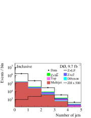
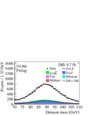
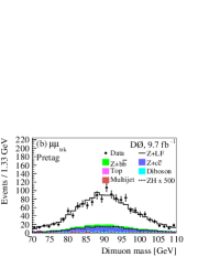
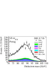
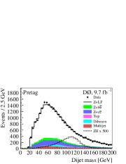
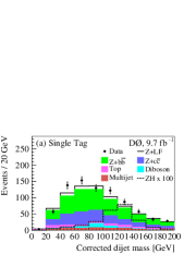
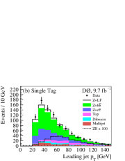
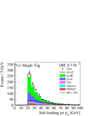
Figure 2 shows the jet multiplicity distribution in the inclusive sample for the combination of all channels. The dimuon and dielectron mass spectra in the pretag sample are shown in Fig. 3. In Figs. 4 and 5, we show distributions of the transverse momenta of the two jets with the highest $p_{\rm T}$ and the invariant mass of the dijet system constructed from those two jets. In all plots, data points are shown with error bars that reflect statistical uncertainty only, and discrepancies in data-MC agreement are within the systematic uncertainties described in Sec. IX.

Figure 2: (color online). Jet multiplicity distribution in the inclusive sample, summed over all lepton channels, along with the background expectation. The signal distribution for $M_{H}=$ 125 GeV is scaled by a factor of 500.

Figure 3: (color online). The dilepton mass spectra, along with the background expectation, for the (a) $\mu\mu$, (b) $\mu\mu_{\rm trk}$, (c) $ee$ and (d) $ee_{\rm ICR}$  channels in the pretag sample. The signal distributions for $M_{H}=$ 125 GeV are scaled by a factor of 500.

Figure 4: (color online). The $p_{T}$ spectra of the (a) leading and (b) sub-leading jets, along with the background expectations, summed over all lepton channels in the pretag sample. The signal distributions, for $M_{H}=$ 125 GeV, are scaled by a factor of 500.

Figure 5: (color online). Distribution of the dijet invariant mass, along with the background expectation, summed over all lepton channels in the pretag sample. The signal distribution, for $M_{H}=$ 125 GeV, is scaled by a factor of 500.

VII Kinematic Fit

We use a kinematic fit to improve the resolution of the dijet invariant mass. The fit varies the energies and angles of the two leptons from the $Z$ boson candidate, and of the two jets that form the Higgs boson candidate (and of a third jet, if present) within their experimental resolutions, subject to three constraints: the reconstructed dilepton mass must be consistent with the $Z$ boson mass and the $x$ and $y$ components of the vector sum of the transverse momenta of the leptons and jets must be consistent with zero.

The fit minimizes a negative log likelihood function:

$$-\ln L_{\mathrm{fit}}=-\sum_{i}\ln f_{i}(y_{i}^{\mathrm{obs}},y_{i}^{\mathrm{pred}})-\sum_{j}\ln C_{j},$$ (2)

where $C_{j}$ ($j=$ 1,2,3) are the probability densities for kinematic constraints, and $f_{i}$ is the probability density (transfer function) for observable $y_{i}^{\mathrm{obs}}$ whose predicted value is $y_{i}^{\mathrm{pred}}$. The fit contains twelve independent observables for events with two jets: four particles $\times$ three variables ($E$ or $1/\mbox{$p_{\rm T}$}$, $\eta$ and $\phi$). For events with three jets, there are fifteen observables.

The probability density for the $Z$ boson mass constraint is a Breit-Wigner function using the values for the mass and width of the $Z$ boson from Ref. pdg . The constraints on the total transverse momentum components are Gaussian distributions with a mean of zero and a width of 7 GeV, as determined from the simulated $ZH$ samples.

We use Gaussian transfer functions for all observables except the energies of the jets. In this case we use three sets of transfer functions, derived from MC studies for: (i) jets that originate from a $b$ quark and do not contain a muon, (ii) jets that originate from a $b$ quark and contain a muon, and (iii) jets that originate from a light quark or gluon. For the jets that form the Higgs boson candidate we use one of the $b$ quark transfer functions, depending on whether they contain a reconstructed muon. For the third jet, if present, we use the light-quark transfer function.

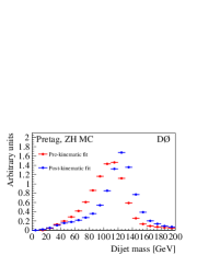
The kinematic fit improves the dijet mass resolution by 10$-$15%, depending on $M_{H}$. The resolution for $M_{H}$ = 125 GeV is approximately 15 GeV (i.e. 12%) after the fit. Distributions of the dijet invariant mass spectra, before and after adjustment by the kinematic fit, are shown in Fig. 6.

Figure 6: (color online). The dijet invariant mass for the simulated $ZH$ signal, at $M_{H}=$ 125 GeV, summed over all lepton channels in the pretag sample, shown before and after the kinematic fit.

VIII Multivariate Analysis

We use a two-step multivariate analysis strategy based on random forest discriminants (RF), an ensemble classifier that consists of many decision trees dtree , as implemented in the tmva software package tmva , to improve the discrimination of signal from background. In a first step, we train a dedicated RF ($t\overline{t}$ RF) that considers $t\overline{t}$ as the only background and $ZH$ as the signal. This approach takes advantage of the distinctive signature of the $t\overline{t}$ background, for instance the presence of large $\not{E}_{\rm T}$. In a second step, we use the $t\bar{t}$ RF output to define two independent regions: a $t\bar{t}$-enriched region and a $t\bar{t}$-depleted region. In each region, we train a global RF to separate the $ZH$ signal from all backgrounds. In both steps we consider ST and DT events separately and train the discriminants for each value of the tested Higgs boson mass in the range $90<M_{H}<150$ GeV in steps of 5 GeV. Compared to the result described in Ref. pubzh , this two-step strategy improves sensitivity to the signal by 5–10%, depending on $M_{H}$.

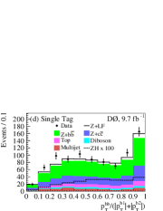
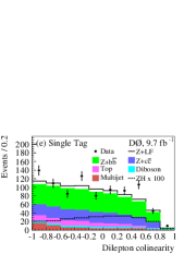
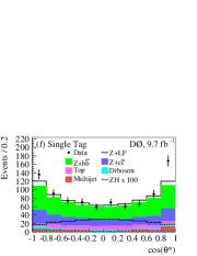
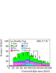
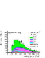
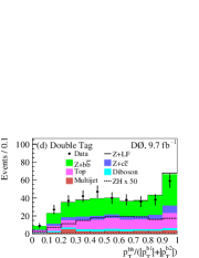
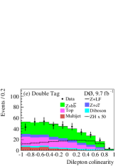
The input variables used for the multivariate analysis include the transverse momenta of the two $b$-jet candidates and the dijet mass, before and after the jet energies are adjusted by the kinematic fit, angular differences between the jets, between the leptons, and between the dijet and dilepton systems, the opening angle between the proton beam and the $Z$ boson candidate in the rest frame of the $Z$ boson, $\cos\theta^{*}$ Parke:1999 , and composite kinematic variables, such as the $p_{\rm T}$ of the dijet system and the scalar sum of the transverse momenta of the leptons and jets. Table 4 provides a complete list of input variables. We show selected distributions of the input variables in Figs. 7 and 8 for ST and DT events, respectively.

Figure 7: (color online). Distributions in ST events of (a) the dijet invariant mass corrected by the kinematic fit, (b) the $p_{T}$ of the leading jet from the Higgs boson candidate, (c) the $p_{T}$ of the sub-leading jet from the Higgs boson candidate, (d) the $p_{T}$ of the dijet system divided by the scalar sum of the transverse momenta of the two jets, (e) the colinearity of the two leptons, and (f) $\cos\theta^{*}$ Parke:1999 . The signal distributions for $M_{H}=$ 125 GeV are scaled by a factor of 100.

Figure 8: (color online). Distributions in DT events of (a) the dijet invariant mass corrected by the kinematic fit, (b) the $p_{T}$ of the leading jet from the Higgs boson candidate, (c) the $p_{T}$ of the sub-leading jet from the Higgs boson candidate, (d) the $p_{T}$ of the dijet system divided by the scalar sum of the transverse momenta of the two jets, (e) the colinearity of the two leptons, and (f) $\cos\theta^{*}$. The signal distributions for $M_{H}=$ 125 GeV are scaled by a factor of 50.

Table 4: Variables used for the $t\overline{t}$ and global RF training. The jets that form the Higgs boson candidate are referred to as $b1$ and $b2$, ordered in $p_{\rm T}$.

variables	$t\bar{t}$ RF	global RF
Invariant mass of the dijet system before (after) the kinematic fit	$\surd$	$\surd$
Transverse momentum of the first jet before (after) kinematic fit	$\surd$	$\surd$
Transverse momentum of the second jet before (after) kinematic fit	$\surd$	$\surd$
Transverse momentum of the dijet system before the kinematic fit	$\surd$	$\surd$
$\Delta\phi$ between the two jets in the dijet system	$-$	$\surd$
$\Delta\eta$ between the two jets in the dijet system	$-$	$\surd$
Invariant mass of all jets in the event	$\surd$	$\surd$
Transverse momentum of all jets in the event	$\surd$	$\surd$
Scalar sum of the transverse momenta of all jets in the event	$\surd$	$-$
Ratio of dijet system $p_{T}$ over the scalar sum of the $p_{T}$ of the two jets ($\mbox{$p_{\rm T}^{bb}$}/(|\mbox{$p_{\rm T}^{b1}$}|+|\mbox{$p_{\rm T}^{b2}$}|)$)	$\surd$	$-$
Invariant mass of the dilepton system	$\surd$	$-$
Transverse momentum of the dilepton system	$\surd$	$\surd$
$\Delta\phi$ between the two leptons	$\surd$	$\surd$
cosine of the angle between the two leptons (colinearity)	$\surd$	$\surd$
$\Delta\phi$ between the dilepton and dijet systems	$\surd$	$\surd$
cosine of the angle between the incoming proton and the $Z$ in the zero momentum frame ($\cos\theta^{*}$) Parke:1999	$-$	$\surd$
Invariant mass of dilepton and dijet system	$-$	$\surd$
Scalar sum of the transverse momenta of the leptons and jets	$-$	$\surd$
Missing transverse energy of the event	$\surd$	$-$
$\not{E}_{\rm T}$ significance met_sig	$\surd$	$\surd$
Negative log likelihood from the kinematic fit (Eq. 1)	$\surd$	$\surd$
$t\overline{t}$ RF output	$-$	$\surd$

To avoid biases in the training procedure, we divide the MC samples into three independent sub-samples: 25% of the events are used to train the RFs (for both the $t\overline{t}$ RF and the global RF); 25% of the events are used to test the RF discrimination performance and check for overtraining (for both the $t\overline{t}$ RF and the global RF), and the remaining 50% of the events (the evaluation sub-sample) are used for the statistical analysis to obtain Higgs boson cross section limits.

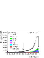
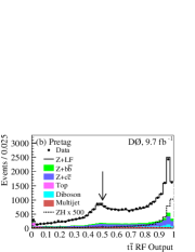
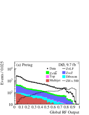
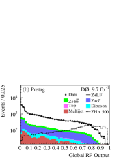
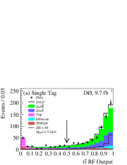
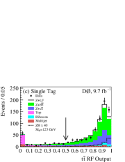
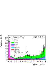
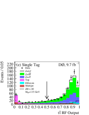
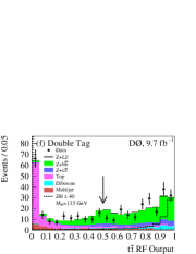
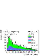
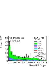
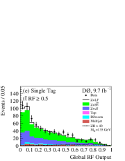
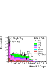
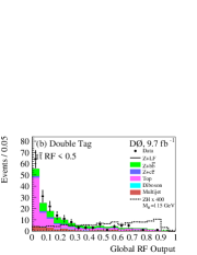
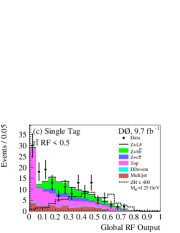
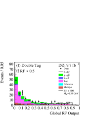
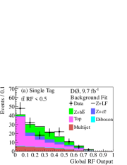
Figures 10 and 10 show the pretag distributions of the $t\overline{t}$ RF and the global RF outputs, respectively, trained for $M_{H}$ = 125 GeV. Figures 11-13 show the corresponding distributions after applying the $b$-tagging requirements for several different values of $M_{H}$. The requirement that separates the $t\overline{t}$-depleted region ($t\overline{t}$ RF $<0.5$) and the $t\overline{t}$-enriched region ($t\overline{t}$ RF $>0.5$) is shown in Figs. 10 and 11.

Figure 9: (color online). The $t\overline{t}$ RF output ($M_{H}=125~{}\mathrm{Ge\kern-1.00006ptV}$) for all lepton channels combined in the pretag sample (a) trained for ST events and (b) trained for DT events. The arrows indicate the $t\overline{t}$ RF selection requirement used to define the $t\overline{t}$-enriched and depleted sub-samples. The signal distributions for $M_{H}=$ 125 GeV are scaled by a factor of 500.

Figure 10: (color online). Global RF output ($M_{H}=125~{}\mathrm{Ge\kern-1.00006ptV}$) for all lepton channels combined for (a) pretag events evaluated with the ST-trained RF and (b) pretag events evaluated with the DT-trained RF. The signal distributions for $M_{H}=$ 125 GeV are scaled by a factor of 500.

Figure 11: (color online). The $t\overline{t}$ RF output for all lepton channels combined in ST and DT events for $M_{H}$ = 115 GeV (a, b), for $M_{H}$ = 125 GeV (c, d), and for $M_{H}$ = 135 GeV (e, f). The signal distributions correspond to the $M_{H}$ used for the RF training and are scaled by a factor of 40. The arrows indicate the $t\overline{t}$ RF selection requirement used to define the $t\overline{t}$-enriched and depleted sub-samples.

Figure 12: (color online). Global RF distributions for ST and DT events in the $t\overline{t}$-depleted region for $M_{H}$ = 115 GeV (a, b), for $M_{H}$ = 125 GeV (c, d), and for $M_{H}$ = 135 GeV (e, f). The signal distributions correspond to the $M_{H}$ used for the RF training and are scaled by a factor of 40.

Figure 13: (color online). Global RF distributions for ST and DT events in the $t\overline{t}$-enriched region for $M_{H}$ = 115 GeV (a, b), for $M_{H}$ = 125 GeV (c, d), and for $M_{H}$ = 135 GeV (e, f). The signal distributions correspond to the $M_{H}$ used for the RF training and are scaled by a factor of 400.

IX Systematic Uncertainties

We assess the impact of systematic uncertainties on both the normalization and shape of the predicted global RF distributions for the signal and for each background source. We summarize the magnitude of these uncertainties in Tables 5 – 7, and provide additional details below. Unless otherwise stated, we consider each source of systematic uncertainty to be 100% correlated for each process across all samples.

The uncertainties on the integrated luminosity and the lepton identification efficiencies are absorbed by the uncertainties on the normalization procedure described in Section VI. The uncertainties on the normalization of the multijet background are determined from the statistical uncertainties on the fit, typically around 10%. These are uncorrelated across channels but are correlated within a channel (i.e., between the different $b$-tag samples, and between the $t\overline{t}$-depleted and enriched regions). We compare the value of $k_{Z}^{2}$ from the combined normalization to the values obtained from independent fits in each channel We assess an uncertainty for each channel that is equal to the RMS (3–5%) of the observed deviations. This uncertainty is taken to be uncorrelated across channels. The normalization of the $Z+$jets background to the pretag data constrains that sample within the statistical uncertainty (1–2%) of the pretag data. Since this sample is dominated by the $Z$+LF background, the normalization of the $t\overline{t}$, diboson, and $ZH$ samples acquires a sensitivity to the inclusive $Z$ boson cross section, for which we assess a 6% uncertainty dyxsec . We assign this uncertainty to these samples as a common uncertainty. We apply a 9% uncertainty to the Run $2$a prediction of $Z+$LF production to account for the different values of $k_{Z}^{2}$ obtained for Run $2$a and Run $2$b. For $Z+$HF production, we evaluate a cross section uncertainty of 20% based on Ref. mcfm . For the diboson and $t\overline{t}$ backgrounds, we take the uncertainties on the cross sections to be 7% mcfm and 10% ttbarxsec , respectively. The cross section uncertainty for the signal is 6% zhxsec .

Sources of systematic uncertainty affecting the shapes of the final discriminant distributions are the jet energy scale, jet energy resolution, jet identification efficiency, and $b$-tagging efficiency. Shape uncertainties are assessed by repeating the full analysis with each source of uncertainty varied by $\pm 1$ s.d. Other sources include trigger efficiency, multijet modeling in the $ee$ channel, PDF uncertainties pdf , data-determined corrections to the model for $Z+$jets, modeling of the underlying event, the MLM matching applied to alpgen $Z$+LF events mlm , and from varying the factorization and renormalization scales for the alpgen $Z+$jets simulation.

Table 5: Systematic uncertainties that are common across all sub-samples. Systematic uncertainties for $ZH$ production shown in this Table are obtained for $M_{H}=125$ GeV. Relative uncertainties are given in percent. When two numbers are given, the first is for Run $2$b and the second is for Run $2$a.

Relative uncertainties (%)

Contribution	$ZH$	Multijet	$Z$+LF	$Z+\mbox{$b\overline{b}$}$	$Z+\mbox{$c\overline{c}$}$	Dibosons	$t\overline{t}$
Multijet Normalization	–	10	–	–	–	–	–
$k^{0}_{Z}$ Uncertainty	1.6 / 6.9	–	–	–	–	1.6 / 6.9	1.6 / 6.9
$k^{2}_{Z}$ Uncertainty	–	–	0.7 / 1.8	0.7 / 1.8	0.7 / 1.8	–	–
$k^{2}_{Z}$ RMS	5.1 / 3	–	5.1 / 3	5.1 / 3	5.1 / 3	5.1 / 3	5.1 / 3
Run $2$a Normalization	– / 9	–	–	–	–	– / 9	– / 9
Theoretical Cross Sections	6	–	–	20	20	7	10
PDFs	0.6	–	1.0	2.4	1.1	0.7	5.9

Table 6: Systematic uncertainties on ST events in the $t\overline{t}$-depleted and enriched regions. Systematic uncertainties for $ZH$ production shown in this Table are obtained for $M_{H}=125$ GeV. Relative uncertainties are given in percent. As these uncertainties change the shape of the global RF distributions, the numbers refer to average per-bin changes. When a range is given, the uncertainty varies by $Z$ boson decay channel.

Relative uncertainties (%) in the $t\bar{t}$-depleted region for ST events

Contribution	$ZH$	Multijet	$Z$+LF	$Z+\mbox{$b\overline{b}$}$	$Z+\mbox{$c\overline{c}$}$	Dibosons	$t\overline{t}$
Jet Energy Scale	0.6	–	3.1	2.3	2.3	4.8	0.3
Jet Energy Resolution	0.7	–	2.7	1.3	1.6	1.0	1.1
Jet Identification	0.6	–	1.5	0.0	0.5	0.7	0.7
Jet Taggability	2.0	–	1.9	1.7	1.7	1.8	2.2
Heavy Flavor Tagging Efficiency	0.5	–	–	1.6	3.9	–	0.7
Light Flavor Tagging Efficiency	–	–	68	–	–	2.9	–
Trigger	0.4–2	–	0.1–2	0.2–2	0.2–2	0.2–2	0.5–2
$Z$ boson $p_{T}$ Model	–	–	1.6	1.7	1.5	–	–
$Z$+jets Jet Angles	–	–	1.7	1.7	1.7	–	–
alpgen MLM	–	–	0.2	–	–	–	–
alpgen Scale	–	–	0.3	0.5	0.5	–	–
Multijet Shape for $ee$ channel	–	45	–	–	–	–	–
Underlying Event	–	–	0.4	0.4	0.4	–	–

Relative uncertainties (%) in the $t\bar{t}$-enriched region for ST events

Contribution	$ZH$	Multijet	$Z$+LF	$Z+\mbox{$b\overline{b}$}$	$Z+\mbox{$c\overline{c}$}$	Dibosons	$t\overline{t}$
Jet Energy Scale	7.5	–	4.6	1.7	3.9	11	2.5
Jet Energy Resolution	0.2	–	4.5	0.7	3.1	3.9	0.7
Jet Identification	1.2	–	2.1	1.0	1.2	0.9	0.7
Jet Taggability	2.1	–	7.3	2.7	3.0	2.0	3.2
Heavy Flavor Tagging Efficiency	0.5	–	–	1.3	4.8	–	0.8
Light Flavor Tagging Efficiency	–	–	73	–	–	4.1	–
Trigger	1–4	–	1–4	0.7–4	0.7–4	1–8	1–8
$Z$ boson $p_{T}$ Model	–	–	3.3	1.5	1.4	–	–
$Z$+jets Jet Angles	–	–	1.7	2.3	2.7	–	–
alpgen MLM	–	–	0.4	–	–	–	–
alpgen Scale	–	–	0.7	0.7	0.7	–	–
Multijet Shape for $ee$ channel	–	59	–	–	–	–	–
Underlying Event	–	–	0.9	1.1	1.1	–	–

Table 7: Systematic uncertainties on DT events in the $t\overline{t}$-depleted and enriched regions. Systematic uncertainties for $ZH$ production shown in this Table are obtained for $M_{H}=125$ GeV. Relative uncertainties are given in percent. As these uncertainties change the shape of the global RF distributions, the numbers refer to average per-bin changes. When a range is given, the uncertainty varies by $Z$ boson decay channel.

$ZH\rightarrow\ell\ell\mbox{$b\overline{b}$}$ Relative uncertainties (%) in the $t\bar{t}$-depleted region for DT events

Contribution	$ZH$	Multijet	$Z$+LF	$Z+\mbox{$b\overline{b}$}$	$Z+\mbox{$c\overline{c}$}$	Dibosons	$t\overline{t}$
Jet Energy Scale	0.5	–	4.6	3.0	1.3	4.5	1.4
Jet Energy Resolution	0.4	–	7.0	1.8	2.9	0.9	0.9
Jet Identification	0.6	–	7.9	0.3	0.5	0.5	0.5
Jet Taggability	1.7	–	7.0	1.5	1.5	3.0	1.7
Heavy Flavor Tagging Efficiency	4.4	–	–	5.0	5.6	–	3.8
Light Flavor Tagging Efficiency	–	–	75	–	–	4.7	–
Trigger	0.4–2	–	0.6–6	0.3–2	0.3–3	0.4–2	0.6–5
$Z_{p_{T}}$ Model	–	–	2.9	1.4	1.9	–	–
$Z$+jets Jet Angles	–	–	1.9	3.5	3.8	–	–
alpgen MLM	–	–	0.2	–	–	–	–
alpgen Scale	–	–	0.4	0.5	0.5	–	–
Multijet Shape for $ee$ channel	–	66	–	–	–	–	–
Underlying Event	–	–	0.5	0.4	0.4	–	–

$ZH\rightarrow\ell\ell\mbox{$b\overline{b}$}$ Relative uncertainties (%) in the $t\bar{t}$-enriched region for DT events

Contribution	$ZH$	Multijet	$Z$+LF	$Z+\mbox{$b\overline{b}$}$	$Z+\mbox{$c\overline{c}$}$	Dibosons	$t\overline{t}$
Jet Energy Scale	6.6	–	0.8	1.6	2.2	5.9	1.5
Jet Energy Resolution	1.4	–	267	1.4	2.1	4.0	0.4
Jet Identification	0.9	–	0.6	0.5	3.6	2.8	0.6
Jet Taggability	2.0	–	0.9	1.6	1.9	3.1	2.1
Heavy Flavor Tagging Efficiency	4.0	–	–	5.1	6.6	–	4.2
Light Flavor Tagging Efficiency	–	–	72	–	–	–	–
Trigger	1–3	–	1–3	0.6–3	0.7–4	0.7–4	1–3
$Z$ boson $p_{T}$ Model	–	–	1.8	1.4	1.5	–	–
$Z$+jets Jet Angles	–	–	1.4	3.7	2.3	–	–
alpgen MLM	–	–	0.5	–	–	–	–
alpgen Scale	–	–	0.8	0.5	0.4	–	–
Multijet Shape for $ee$ channel	–	91	–	–	–	–	–
Underlying Event	–	–	0.9	0.7	0.5	–	–

X Results

We use the global RF output distributions of the four sub-samples (ST and DT in the $t\overline{t}$-depleted and $t\overline{t}$-enriched regions) in each channel along with the corresponding systematic uncertainties to extract results for both Higgs boson production and diboson production. The use of separate channels and sub-samples takes advantage of the sensitivity from the signal-rich sub-samples and allows for a better background assessment based on the signal-poor sub-samples. The binning of each distribution is chosen such that the statistical uncertainty for each bin is less than 20% for the signal-plus-background prediction and 25% for the background-only prediction.

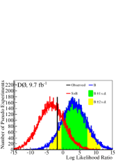
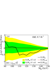
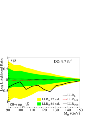
We evaluate the consistency of the data with the background-only ($B$) and signal-plus-background ($S+B$) hypotheses using a modified frequentist (CL_S) method cls . This method uses the negative log likelihood ratio $LLR=-2\ln(L_{S+B}/L_{B})$, where $L_{S+B}$ and $L_{B}$ are the Poisson likelihoods for the $S+B$ and the $B$ hypotheses, respectively.

We combine our results by summing the $LLR$ over all bins of all contributing channels and sub-samples. The signal and background predictions are functions of nuisance parameters that account for the presence of systematic uncertainties. We maximize $L_{S+B}$ with respect to the $S+B$ hypothesis and $L_{B}$ with respect to the $B$ hypothesis with independent fits that allow the sources of nuisance parameters to vary within Gaussian priors wade . The maximized values of $L_{B}$ and $L_{S+B}$ are then used in the calculation of the $LLR$.

We integrate the $LLR$ distributions obtained from $B$ and $S+B$ pseudo-experiments to obtain the $p$-values $CL_{B}$ and $CL_{S+B}$ for the two hypotheses. If the data are consistent with the $B$ hypothesis, we exclude values of the product of the $ZH$ production cross section and branching ratios for which $CL_{S}~{}=~{}CL_{S+B}/CL_{B}<0.05$ at the 95% C.L.

X.1 Results for Diboson Production

To validate the search procedure, we search for $ZZ$ production in the $\ell^{+}\ell^{-}\mbox{$b\overline{b}$}$ final state. We use the same event selection, corrections to our background models, normalization fit parameters, RF training procedure, and statistical analysis methods as for the $ZH$ search. Our search also includes contributions from $ZZ\rightarrow\ell^{+}\ell^{-}\mbox{$c\overline{c}$}$ and $WZ$ production in the $\mbox{$c\overline{s}$}\ell^{+}\ell^{-}$ final state where the $c$ jet passes the $b$-tagging requirement. We collectively refer to them as $VZ$ production. The $WW$ process is considered to be background.

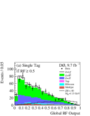
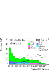
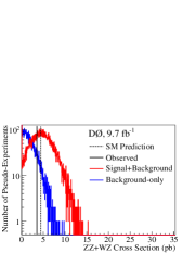
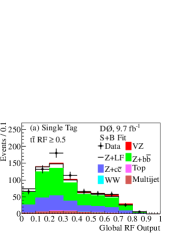
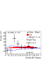
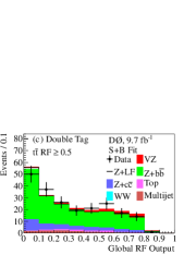
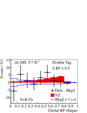
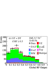
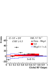
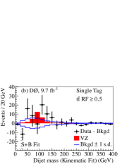
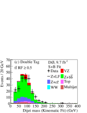
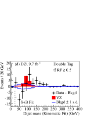
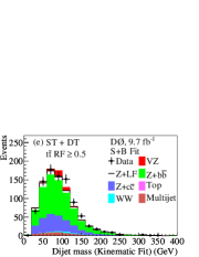
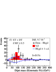
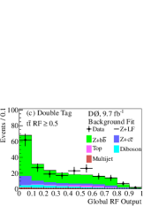
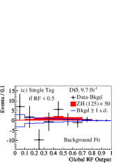
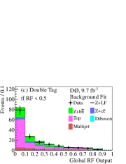
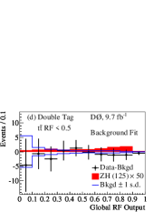
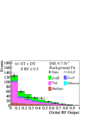
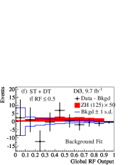
Figure 14 compares the $LLR$ value observed in the data to distributions obtained from $B$ and $S+B$ pseudo-experiments. To obtain $\sigma_{VZ}$ in units of the SM value, we maximize $L_{S+B}$ with respect to the nuisance parameters and a signal scale factor $f$, keeping the ratio of the $ZZ$ and $WZ$ cross sections fixed to the SM prediction. We find $f=0.8\pm 0.6$, which translates to $\sigma_{VZ}=3.5\pm 2.5$ pb given the predicted total SM cross section of $\sigma_{VZ}=4.4\pm 0.3~{}\text{pb}$ mcfm . Figure 15 compares this result to the SM cross section and to the distribution of results obtained from $B$ and $S+B$ pseudo-experiments. The probability ($p$-value) that the $B$ hypothesis results in a cross section greater than that determined from the data is 0.071, equivalent to 1.5 standard deviations (s.d.). The expected $p$-value is 0.032, corresponding to 1.9 s.d. In Figs. 16 and 17 we show the global RF and post-kinematic fit dijet mass distributions after the likelihood fit, separately for ST and DT events in the $t\overline{t}$-depleted region. The diboson signal consists of 66% (93%) $ZZ$ production and 34% (7%) $WZ$ production in the ST (DT) sample.

Figure 14: (color online). $LLR$ distributions obtained from $B$ and $S+B$ pseudo-experiments, using the global RF output as the final variable, for the $VZ$ search. The vertical line indicates the $LLR$ obtained from the data.

Figure 15: (color online). Distribution of $VZ$ cross sections obtained from $B$ and $S+B$ pseudo-experiments. The observed cross section from the data and the SM cross section are also shown.

Figure 16: (color online). Global RF output distributions for the $VZ$ search after the fit to data in the $S+B$ hypothesis in (a) ST events, (c) DT events, and (e) ST and DT events combined. Distributions are summed over all $Z\to\ell\ell$ channels. The $VZ$ signal distribution, scaled to the measured $\sigma_{VZ}$, is compared to the data after subtracting the fitted background in (b) ST events, (d) DT events, and (e) ST and DT events combined. Data points are shown with Poisson statistical errors. Also shown is the uncertainty on the background after the fit.

Figure 17: (color online). Dijet invariant mass distributions for the $VZ$ search after the kinematic fit and after the fit to the data in the $S+B$ hypothesis in (a) ST events, (c) DT events, and (e) ST and DT events combined. Distributions are summed over all $Z\to\ell\ell$ channels. The $VZ$ signal distribution, scaled to the measured $\sigma_{VZ}$, is compared to the data after subtracting the fitted background in (b) ST events, (d) DT events, and (e) ST and DT events combined. Also shown is the uncertainty on the background after the $S+B$ fit.

X.2 Higgs Boson Search Results

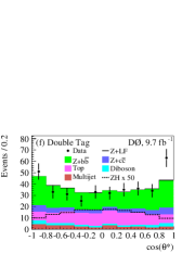
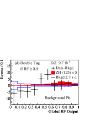
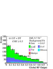
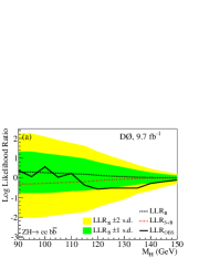
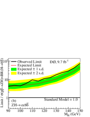
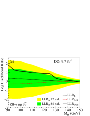
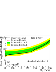
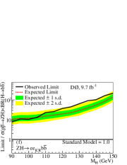
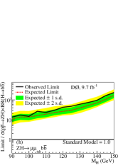
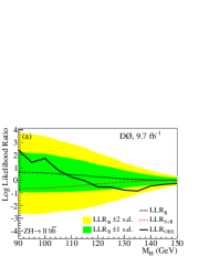
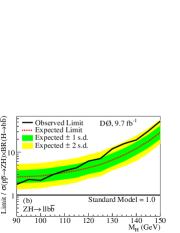
In Figs. 18 and 19 we show the global RF distributions for $M_{H}=125~{}\mathrm{Ge\kern-1.00006ptV}$ after the fit of the nuisance parameters to the data in the $B$ hypothesis. Figure 20 shows the observed and expected (median) $LLR$ values for the individual analysis channels. Also shown are the upper limits at the 95% C.L. on the product of the $ZH$ production cross section and branching ratio for $H\to\mbox{$b\overline{b}$}$. The $LLR$ values for all lepton channels combined are shown in Fig. 21(a), and limits are shown in Fig. 21(b) and Table 8. The limits are expressed as a ratio to the SM prediction. At $M_{H}=125~{}\mathrm{Ge\kern-1.00006ptV}$ the observed (expected) limit on this ratio is 7.1 (5.1).

Table 8: The expected and observed upper limits at the 95% C.L. on the SM Higgs boson production cross section for $ZH\rightarrow\ell^{+}\ell^{-}b\bar{b}$, expressed as a ratio to the SM cross section.

$M_{H}~{}(\mathrm{Ge\kern-1.00006ptV})$	90	95	100	105	110	115	120	125	130	135	140	145	150
Expected	2.6	2.7	2.8	3.0	3.4	3.7	4.3	5.1	6.6	8.7	12	18	29
Observed	1.8	2.3	2.2	3.0	3.7	4.3	6.2	7.1	12	16	19	31	53

Figure 18: (color online). Global RF output distributions in the $t\overline{t}$-depleted region, assuming $M_{H}=$ 125 GeV, after the fit to the data in the $B$ hypothesis for (a) ST events, (c) DT events, and (e) ST and DT events combined. Background-subtracted distributions for (a), (c), and (e) are shown in (b), (d), and (f), respectively. Signal distributions for $M_{H}=$ 125 GeV are shown with the SM cross section scaled by a factor of $5$ in (b), (d), and (f).

Figure 19: (color online). Global RF output distributions in the $t\overline{t}$-enriched region, assuming $M_{H}=$ 125 GeV, after the fit to the data in the $B$ hypothesis for (a) ST events, (c) DT events, and (e) ST and DT events combined. Background-subtracted distributions for (a), (c), and (e) are shown in (b), (d), and (f), respectively. Signal distributions for $M_{H}=$ 125 GeV are shown with the SM cross section scaled by a factor of $50$ in (b), (d) and (f).

Figure 20: (color online). Observed and expected $LLR$ values for the $S+B$ and $B$ hypotheses, along with the $\pm 1$ and $\pm 2$ s.d. bands for the $B$ hypotheses, as well as observed and expected cross section upper limits (along with the $\pm 1$ and $\pm 2$ s.d. bands for the expected limit) relative to the SM cross section, (a, b) for the $ee$ channel, (c, d) for the $\mu\mu$ channel, (e, f) for the $ee_{\rm ICR}$ channel, and (g, h) for the $\mu\mu_{\rm trk}$ channel.

Figure 21: (color online). (a) Observed and expected $LLR$ values as a function of $M_{H}$ for the $S+B$ and $B$ hypotheses, along with the $\pm 1$ and $\pm 2$ s.d. bands for the $B$ hypotheses, for all lepton channels combined. (b) Expected and observed cross section upper limits at the 95% C.L. for $ZH\rightarrow\ell^{+}\ell^{-}b\bar{b}$ production, relative to the SM cross section.

XI Summary

In summary, we have searched for SM Higgs boson production in association with a $Z$ boson in the final state of two charged leptons (electrons or muons) and two $b$-quark jets using 9.7 fb^-1 of $p\bar{p}$ collisions at $\sqrt{s}$ = 1.96 TeV. To validate the methods used in this analysis, we have determined the cross section for $ZZ$ production in the same final state and found it to be a factor of $0.8\pm 0.6$ relative to the SM prediction, with a significance of 1.5 s.d. We have set an upper limit on the product of the $ZH$ production cross section and branching ratio for $H\to\mbox{$b\overline{b}$}$ as a function of $M_{H}$. The observed (expected) limit at the 95% C.L. for $M_{H}=125$ GeV is 7.1 (5.1) times the SM expectation.