Carbon Abundances for Red Giants in the Draco Dwarf Spheroidal Galaxy

Abstract

Measurements of [C/Fe], [Ca/H], and [Fe/H] have been derived from Keck I LRISb spectra of 35 giants in the Draco dwarf spheroidal galaxy. The iron abundances are derived by a spectrum synthesis modeling of the wavelength region from 4850 to 5375 Å, while calcium and carbon abundances are obtained by fitting the Ca II H and K lines and the CH G band respectively. A range in metallicity of $-2.9\leq{\rm[Fe/H]}\leq-1.6$ is found within the giants sampled, with a good correlation between [Fe/H] and [Ca/H]. The great majority of stars in the sample would be classified as having weak absorption in the $\lambda$3883 CN band, with only a small scatter in band strengths at a given luminosity on the red giant branch. In this sense the behavior of CN among the Draco giants is consistent with the predominantly weak CN bands found among red giants in globular clusters of metallicity ${\rm[Fe/H]}<-1.8$. Over half of the giants in the Draco sample have ${\rm[Fe/H]}>-2.25$, and among these there is a trend for the [C/Fe] abundance to decrease with increasing luminosity on the red giant branch. This is a phenomenon that is also seen among both field and globular cluster giants of the Galactic halo, where it has been interpreted as a consequence of deep mixing of material between the base of the convective envelope and the outer limits of the hydrogen-burning shell. However, among the six Draco giants observed that turn out to have metallicities $-2.65<{\rm[Fe/H]}<-2.25$ there is no such trend seen in the carbon abundance. This may be due to small sample statistics or primordial inhomogeneities in carbon abundance among the most metal-poor Draco stars. We identify a potential carbon-rich extremely metal-poor star in our sample. This candidate will require follow up observations for confirmation.

1 Introduction

The Draco dwarf spheroidal (dSph) galaxy is chemically inhomogeneous. A spread in heavy element abundance was first revealed by the spectrophotometric study of Zinn (1978) and confirmed by the low-resolution spectroscopy of Kinman et al. (1980), Stetson (1984), and Smith (1984). The inhomogeneities are present across a range of elements including Ca (Lehnert et al. 1992; Winnick 2003; Smith et al. 2006), other $\alpha$ elements, and the iron-peak elements (Shetrone et al. 1998a, 2001a; Cohen & Huang 2009; Kirby et al. 2010). Draco has an integrated visual luminosity of $L_{V}=2.6\times 10^{5}L_{\odot}$ (Mateo 1998), such that its luminosity and stellar mass are comparable to those of a medium-mass globular cluster (Hodge 1964). The general element spread within Draco and other dSphs has been interpreted as the result of internal chemical evolution (Zinn 1978; Ikuta & Arimoto 2002; Winnick 2003; Marcolini et al. 2006; Cohen & Huang 2009; Kirby et al. 2011a, 2011b). The presence of dark matter halos in dSphs such as Draco (Pryor & Kormendy 1990; Armandroff et al. 1995; Kleyna et al. 2001, 2002; Mashchenko et al. 2006) can help account for why systems of such low stellar mass can have sustained a prolonged episode of element buildup by retaining ejecta from evolving stars and/or by capturing new gas. Dwarf spheroidals are now playing a major role in the context of the hierarchical formation and evolution of galaxies, and their internal abundance patterns are providing insights into how such evolution took place (e.g., Shetrone et al. 2001a; Geisler et al. 2005; Robertson et al. 2005; Kirby et al. 2008; Frebel et al. 2010).

A contrast between the Draco dSph and globular clusters of similar luminous mass is striking because clusters of this mass are generally very homogeneous in many of the $\alpha$ and Fe-peak elements that are inhomogeneous in Draco. The CNO group elements are a notable exception, since inhomogeneities in the isotopes of this element group are commonplace within globular clusters, even in clusters of lower stellar mass than the Draco dSph. Concerning carbon and nitrogen certain distinctive patterns have been discerned within globular clusters. Stars of similar effective temperature and luminosity within the same cluster can exhibit very different strengths of the $\lambda$3883 or $\lambda$4215 CN band in the spectrum (e.g., Norris & Smith 1981). The fact that such differences occur among main sequence stars within a cluster, as first found by Hesser (1978), suggests that they date from very early times in cluster history, perhaps originating from a period of cluster chemical evolution instigated by stars more massive than the present main sequence turnoff stars. Among stars on the upper part of the red giant branch (RGB) there is an apparently separate phenomenon that is evinced as a decline in mean surface carbon abundance with increasing stellar luminosity (e.g., Kraft 1984). The inference is that some interior mixing process is at work within such stars to transport material from the vicinity of the hydrogen-burning shell to the base of the convective envelope, whereupon it can be rapidly convected to the stellar surface. See Gratton et al. (2012) for a more extensive review of this subject.

There is much less known about the CN and CH distributions within dwarf spheroidal galaxies than within globular clusters. Norris et al. (2010) have a moderate number of stars with carbon abundances in the Bootes and Segue I systems but the stars in these ultra faint dwarf galaxies are extremely metal-poor and may not serve as a guide for what the carbon evolution may look like in a more massive ”classical” dwarf galaxy. If the CN inhomogeneities within clusters are of a primordial origin, then it is of interest to know whether they are present within the different environments of dSph systems. Dwarf spheroidals are known to have both metallicity spread and a spread in ages (see the recent review by Tolstoy et al. 2009). The spread in metallicity may mean that the most metal-poor stars may have a different primordial origin for the C and N compared to the more metal-rich stars. In addition, some observations and models, e.g. Revaz et al. (2009), suggest that in some dwarf galaxies there may be a spread of ages at a single metallicity. As a final complication, there are carbon depletions of luminous cluster red giants that are the product of a stellar interior mixing process that appears to also function within halo field red giants of the Milky Way. If the mixing process is a fundamental attribute of the evolution of low-mass metal-poor stars then it would also be expected to occur among red giants in the dwarf spheroidal satellites of the Galaxy. With such questions in mind, the present paper reports upon an observational study of CN and CH bands in the spectra of red giants in the Draco dwarf spheroidal system.

In the Galactic halo a very significant fraction of extremely metal-poor stars is carbon enhanced, recently measured to be as high as 32% by Yong et al. (2012) for stars with ${\rm[Fe/H]}<-3$. In general the fraction is supposed to decrease with increasing metallicities, but several studies still find high fractions for stars just outside the extremely-low metallicity regime (25% for ${\rm[Fe/H]}<-2.5$ by Marsteller et al. 2005, at least 21% for ${\rm[Fe/H]}<-2.0$ by Lucatello et al. 2006, and 14% for ${\rm[Fe/H]}<-2.0$ by Cohen et al. 2005). In recent work by Starkenburg et al. (2011) carbon measurements were compiled for nine stars with ${\rm[Fe/H]}<-2.5$ in the Sculptor dSph (seven of which have ${\rm[Fe/H]}<-3.0$), and none of these stars was found to be carbon enhanced. Based on this sample of nine stars, Starkenburg et al. estimated that there is a low probability of $\sim$ 2% – 13% that the lack of carbon enhanced stars in Sculptor is entirely a chance effect. Thus carbon may vary from star to star at a given metallicity for several reasons within dSphs such as Draco, and determining the general trends and the reasons why the exceptions stand out requires a large sample.

2 Observations and Reductions

Spectra of 35 red giants in the Draco dwarf spheroidal were obtained with the blue channel of the LRIS spectrograph (Oke et al. 1995; McCarthy et al. 1998) on the Keck I telescope. This blue channel is denoted as LRISb throughout this paper. Observations were made using the multi-object mode of LRISb in which the single long-slit assembly is replaced by a slit mask. The results reported in this paper are based on observations acquired on UT 2007 June 19 of two different slit mask fields. Each slit mask field was exposed on for a total of five 1800 s integrations. Since LRIS is a dual-channel spectrometer a mirror was used in place of a dichroic to reflect all light to the LRISb side. The dispersive element employed for the spectroscopy was the 400/3400 grism, and the detector was a $2\times 2{\rm K}\times 4{\rm K}$ Marconi E2V CCD with 15 $\mu$m pixels. Sky conditions were clear. As determined by the emission lamp lines the delivered resolution was 630. Because we used slit masks the wavelength coverage varied depending upon the slit position within the field but for those slits in the middle of the mask produced spectra covering the entire optical range.

Basic astrometric and photometric properties of the stars observed are given in Table 1. Stars can be identified via the right ascensions and declinations listed. Column 1 of the table gives the identification assigned here, whereas Column 2 lists alternative designations from Baade & Swope (1961), Stetson (1984) and Winnick (2003). Infrared photometry in Table 1 is obtained from the 2MASS catalog for the $J$, $H$ and $K_{s}$ bands. Metallicities derived by Winnick (2003) are listed in the Column headed ${\rm[Fe/H]}_{\rm CaT}$ in Table 1.

Optical photometry for members of Draco in our program is based on CCD frames obtained by H. E. Bond with the Kitt Peak National Observatory 0.9 m telescope on 1996 September 22. The T2KA chip at the Ritchey-Chretien focus provides a $23^{\prime}\times 23^{\prime}$ field, which encloses the core of the galaxy ($r_{c}=9^{\prime}$; Irwin & Hatzidimitriou 1995). A combination of $BVI$ filters was used with exposure times of 300, 180, and 300 s, respectively, under photometric conditions. The photometry was calibrated to the network of $BVI$ standard stars established by Siegel & Bond (2005). Data were reduced using the IRAF CCDPROC pipeline and photometry was measured with DAOPHOT/ALLSTAR (Stetson 1987, 1994). DAOGROW (Stetson 1990) was used to perform curve-of-growth fitting for aperture correction on both program and standard stars. The raw photometry was calibrated using the iterative matrix inversion technique described in Harris et al. (1981) and Siegel et al. (2002) to translate the photometry to the standard system of Landolt (1992) and Siegel & Bond (2005). The $V$ magnitudes plus $(B-V)$ and $(V-I)$ colors derived from this photometry for the Draco program stars are listed in Table 1.

The color-magnitude diagram (CMD) of the observed Draco sample is plotted in Figure 1, based on the $(V,B-V)$ photometry from Table 1. A linear least-squares (lsq) fit to the sequence defined by this sample has the equation $V_{\rm lsq}=21.655-3.402(B-V)$, and is shown by the solid line in the figure. The standard deviation in the slope of this relation is 0.291. Each star presents a color residual $\Delta(B-V)=(B-V)-(B-V)_{\rm lsq}$ with respect to this lsq fit. In a chemically inhomogeneous system these color residuals would be expected to correlate with stellar metallicity, an expectation that is testable with the data.

The spectra were reduced using iraf 2dspec routines. To set the final velocity/wavelength scale the blended stellar lines in the spectra themselves were used. The position of each line was determined (using splot in IRAF) from a synthetic spectrum convolved to the resolution of LRISb with stellar parameters typical of our sample stars. Although flux standard stars were observed with the LRIS long slit, the spectra cover a different wavelength range than some of the observed spectra, and thus were of limited use for fluxing the data. Fluxing was done after the final abundance analysis was completed and is discussed in the following section.

3 Abundance Analysis and Indices

3.1 Stellar Parameters

For this analysis we used photometric surface gravities and effective temperatures and metallicities from the red portion of the spectrum (see Section 3.2 for this procedure). As an initial guess we used the metallicities from Winnick (2003) for the 25 stars in common. Winnick (2003) used a metallicity calibration from the calcium triplet lines to obtain metallicities for the Draco dSph giants. For those stars without a metallicity estimate we began with a metallicity of ${\rm[M/H]}=-2$. When an initial estimate of the metallicity was more than 0.15 dex different from the derived low resolution metallicity another iteration was made with a second determination of effective temperature and surface gravity.

Effective temperatures were obtained for stars in the sample by using metallicities, photometry and the calibrations of Ramírez & Meléndez (2005) and a reddening of $E(B-V)=0.03$. The values of $T_{\rm eff}$ listed in Column 8 of Table 2 are an average of the temperatures obtained using the $(V-I)$, $(B-V)$, $(V-J)$, $(V-H)$, and $(V-K)$ calibrations, after potentially iterating if the initial guess of the metallicity was not sufficiently accurate.

The surface gravity was obtained using the standard equation:

$${\rm log}\,g={\rm log}\,g_{\odot}+{\rm log}(M/M_{\odot})+0.4(M_{\rm{bol}}-M_{\rm{bol}\odot})+4\,{\rm log}(T_{\rm{eff}}/T_{{\rm eff}\odot}),$$ (1)

where the bolometric magnitude is given by

$$M_{\rm bol}=V-(m-M)_{V}+BC_{V}.$$ (2)

The distance modulus, $(m-M)_{V}$, was adopted as 19.65, $M_{{\rm bol}\odot}=4.75$ , $\log g_{\odot}=4.44$ cgs, $T_{{\rm eff}\odot}=5790K$. The bolometric correction $BC_{V}(T_{\rm eff}$) was taken from Alonso et al. (1999).

The microturbulence was determined from a calibration of the Lick-Texas group (e.g., Kraft & Ivans 2003) analyses of globular cluster giants and the DART (Tolstoy et al. 2006) analyses of dSph giants as follows:

$$v_{t}=-0.41\log g+2.15,$$ (3)

where $v_{t}$ is in km s^-1 and $g$ is in cgs. Values of surface gravity and microturbulence velocity adopted for each Draco star to be analyzed are listed in Columns 10 and 11 respectively of Table 2.

3.2 Analysis Procedure

The line list used for this project includes atomic, C₂, CN, SiH, and MgH lines from the Kurucz compilation (http://kurucz.harvard.edu/LINELISTS/GFHYPERALL). The CH line list came from B. Plez 2010 (private communication). Model atmospheres were computed without convective overshooting from the Kurucz (1993) grid, using interpolation software developed by A. McWilliam 2009 (private communication).

Synthetic spectra were computed using the 2010 scattering version of MOOG (Sneden 1973, Sobeck et al. 2011). The standard version of MOOG treats continuum scattering ($\sigma_{\nu}$) as if it were absorption ($\kappa_{\nu}$) in the source function, i.e., $S_{\nu}=B_{\nu}$ (the Planck function), an approximation that is only valid at long wavelengths. At shorter wavelengths, Cayrel et al. (2004) have shown that the scattering term must be taken into account such that the source function becomes $S_{\nu}=(\kappa_{\nu}B_{\nu}+\sigma_{\nu}J_{\nu})/(\kappa_{\nu}+\sigma_{\nu})$. For metal-poor red giants, the difference in iron line abundances usually becomes notable ($>0.05$ dex) below 5000 Å. The scattering corrections are negligible for red lines ($>5000$ Å), but can approach 0.4 dex for resonance lines in the blue.

Some assumptions about element abundance ratios were needed for the analysis. For oxygen and the other alpha elements the abundances were assumed to be [$\alpha$/Fe]=[Ca/Fe], although the choice of [O/Fe] had little impact on the final carbon determination (a change of [O/Fe] of 0.3 dex from that assumed by setting [O/Fe] = [Ca/Fe] causes the derived [C/Fe] to change by 0.06 dex). The carbon isotope ratio was assumed to be ${\rm C}^{12}/{\rm C}^{13}=10$. Little is known regarding the isotopic carbon ratio among red giants in dwarf galaxies so we adopt a value between that found among the brightest halo red giants and those near the bump in the luminosity function, see Gratton et al. (2000) for field stars and Smith et al. (2007), Shetrone (2003) and Recio-Blanco & de Laverny (2007) for globular cluster stars.

The iron abundance was determined from the 4850-5375 Å region by using a spectrum synthesis approach. Synthetic spectra with different iron abundances were compared to an observed spectrum, excluding regions with bad sky subtraction or cosmic rays. The abundance is taken from the synthetic spectrum that produced the smallest residuals about a constant value that was allowed to vary from comparison to comparison to compensate for errors in the continuum normalization.

The [Ca/Fe] abundance was determined from the Ca II H and K lines via a technique similar to that used to determine the iron abundance except that the [Ca/H] abundance was now allowed to vary instead of [Fe/H]. Three pixels at the core of both the H and K lines were excluded from the comparisons since those regions were found to be not well fit by the model atmospheres and techniques used.

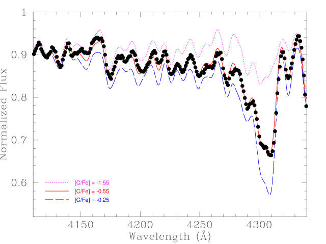
Figure 2: The normalized spectrum for star 161 (star 3157 in Cohen & Huang 2009). The black dots represent the observed spectra and the three lines are synthetic spectra with different [C/Fe] ratios.

After [Fe/H] and [Ca/H] were determined the G band at $\sim 4300$ Å was modeled to derive carbon abundances using the same techniques that were applied to the 4850-5375 Å region for iron abundance measurement except that only carbon was allowed to vary. Figure 2 shows a small section of the observed spectrum for star 161, displayed as the black points, along with several synthetic spectra with different [C/Fe] ratios.

The [Fe/H], [Ca/H] and [C/Fe] abundances derived from the synthetic spectra analyses of the LRISb spectra are listed in Columns 4, 6 and 8 of Table 2. A low order polynomial fit of the initial spectrum divided by the final synthetic spectrum was divided back into the initial spectrum to produce the final normalized observed spectrum.

3.3 Error Analysis

Four stars, denoted 361, 409, 410, 427 in Table 1, were observed through both of the slit masks employed. These multiple observations allow us to compare the abundance results for internal consistency. The average of differences in [Fe/H], [Ca/H], and [C/Fe] between these observed pairs is 0.04, 0.05, and 0.10 dex, respectively. Our estimate for the typical fitting (measurement) errors for these three abundances are 0.08, 0.06, and 0.05 dex, respectively.

The formal internal error of the mean of the effective temperatures is small. In order to look for systematic and external errors we compared the temperatures derived in this work with spectroscopic temperatures derived in the high resolution analyses of Shetrone et al. (2001a) and Cohen & Huang (2009) for five stars that we have in common. Our temperatures are 33 $\pm$ 56 K cooler than the literatures values with a standard deviation of 110 K. This standard deviation is far larger than the internal errors on the photometric effective temperature for these stars. Thus we inflate our internal scatter error by 80 K (combined in quadrature) to cover the possible external errors. These modified temperature errors $\epsilon(T_{\rm eff})$ are listed in Column 12 of Table 2.

The uncertainty on the abundances were determined using the standard practice of propagating the uncertainties in stellar parameters and combining in quadrature. The temperature was varied by the amount listed in Column 12 of Table 2. The gravity and microturbulence were varied by 0.2 dex and 0.3 km s^-1 respectively. Since [Fe/H] is relatively insensitive to mistakes in the model atmosphere metallicity the error in the model metallicity can be formulated by combining the error in gravity, temperature and microturbulence for [Fe/H]. By contrast, [Ca/H] and [C/Fe] are more sensitive to errors in the model atmosphere metallicity thus we also include the error in [Fe/H] along with the errors in gravity, microturbulence and effective temperature in the quadrature sum. With each new model the features were refit and new abundances determined. This analysis was performed for several stars spanning the range in temperature and metallicity of the Draco sample, resulting in an average error formula for [C/Fe] of $\epsilon{\rm[C/Fe]}=[0.0194+(\epsilon{\rm[Fe/H]})^{2}+(0.0005\times\epsilon(T_{\rm eff}))^{2}]^{1/2}$ and $\epsilon{\rm[Ca/H]}=[0.0013+(0.4\times\epsilon{\rm[Fe/H]})^{2}+(0.0006\times\epsilon(T_{\rm eff})^{2}]^{1/2}$ for [Ca/H]. The uncertainties thereby computed for the [Fe/H], [Ca/H] and [C/Fe] abundances are listed in Columns 5, 7 and 9 respectively of Table 2.

3.4 Comparisons with Other Abundances

The veracity of the [Fe/H] abundances from Column 4 of Table 2 can be tested via several comparisons. The first comparison is shown in Figure 3, in which [Ca/H] as derived from the Ca II H and K lines is plotted versus [Fe/H] from Fe I lines. There is a clear correlation with a slight offset in the sense that [Ca/H] is systematically $\sim 0.05$ dex greater than [Fe/H] except at the highest metallicities in the sample with ${\rm[Fe/H]}>-1.8$. Various symbols are used in Figure 3 to denote three different metallicity ranges based on the LRISb [Fe/H] abundances: filled squares (${\rm[Fe/H]}<-2.25$), filled circles ($-2.25\leq{\rm[Fe/H]}\leq-1.85$), and filled triangles (${\rm[Fe/H]}>-1.85$). These symbols for stars of different metallicity are also used in other figures of this paper.

Winnick (2003) derived [Fe/H] for a large sample of Draco giants from calibrating the strength of the Ca II near-infrared triplet lines. There are 25 stars in our Draco program for which Winnick derived such abundances, that are denoted here as ${\rm[Fe/H]}_{\rm CaT}$ (Table 1). A plot of ${\rm[Fe/H]}_{\rm CaT}$ versus the [Fe/H] abundances from Column 4 of Table 2 is presented in Figure 4. By and large the comparison is quite favorable, with the data scattering about the line corresponding to equality. The LRISb metallicities are identical with ${\rm[Fe/H]}_{\rm CaT}$ to within the 0.03 dex error on the mean difference (the standard deviation being 0.17 dex). There is perhaps a tendency for the Ca triplet values of [Fe/H] (as calibrated by Winnick) to be systematically less than the LRISb abundances by $\sim 0.1$ dex for the lowest-metallicity stars in the sample. This is not entirely surprising as more recent non-linear calibrations for the Ca triplet have been suggested for very metal-poor stars, see Starkenburg et al. (2010).

Iron abundances have been measured from medium-resolution spectra for several of the stars in Table 2 by Kirby et al. (2010). The comparison between the Kirby et al. [Fe/H] values and our sample is given in Table 3 and shown in Figure 4 as blue triangles. The general agreement is very good ($+0.04\pm 0.05$, $\sigma=0.16$). A comparison can also be made based on a small overlap with high-resolution studies by Shetrone et al. (2001a), Fulbright et al. (2004), and Cohen & Huang (2009). In the case of the three giants with high-resolution abundances of ${\rm[Fe/H]}<-2.0$ dex the agreement with the LRISb-based [Fe/H] values is excellent ($-0.05\pm 0.06$ dex). However, for the two more metal rich giants (187 and 240) the agreement is quite poor, with the LRISb [Fe/H] values being $0.39\pm 0.01$ less than those of Shetrone et al. (2001a). The cause of this larger discrepancy is not known. The agreement between our [Ca/Fe] abundance ratios and those in the two high resolution samples is excellent ($-0.04\pm 0.06$).

Another check upon the [Fe/H] abundances from Table 2 is to see whether they correlate with the position of stars on the RGB of the CMD of Draco. The color residual $\Delta(B-V)$ defined in Section 2 is plotted in Figure 5 versus the LRISb [Fe/H] abundance from Column 4 of Table 2. A correlation is evident, albeit with notable scatter. One interpretation of Figure 5 might be that the relation between metallicity and color on the RGB of Draco is not 1-to-1, particularly among the lowest metallicity giants. This complication was first discussed by Stetson (1980) and Zinn (1980). In a system such as Draco in which there is a metallicity spread it can be hard to distinguish between RGB and asymptotic giant branch (AGB) stars, making it more difficult to interpret any relation between color and metallicity. Scatter in Figure 5 can also result from another source, namely that the linear fit in Figure 1 does not properly represent the curvature of the RGB in the CMD. This could be particularly important for stars at the fainter end of our sample where the locus of the RGB is becoming steeper than at higher luminosities. Other potential sources of confusion between color and metallicity are spreads in age and a spread in the [$\alpha$/Fe] abundance ratio (both as a function of metallicity and at a fixed metallicity).

There are very few studies of [C/Fe] in dwarf galaxies. Cohen & Huang (2009) have a sample of eight stars, one of which we have also observed. That star in common is star 161, called 3157 in Cohen & Huang (2009) and shown in Figure 2. We determine a [C/Fe] of $-0.55$ while Cohen & Huang (2009) derive $-0.29$. The solar Fe and C abundances adopted by Cohen & Huang (2009) are 7.45 and 8.59, respectively, while we use the default Fe and C abundance found in MOOG, i.e., 7.52 and 8.56. When this is accounted for the discrepancy is reduced slightly, from 0.26 to 0.22 dex. As a further test we used the Cohen & Huang (2009) stellar parameters for star 161 and recovered their preferred [C/Fe] abundance to within our measurement error of 0.05 dex. This shows that our technique and spectra can derive abundances having an accuracy dominated by modeling and systematic errors.

4 Indices

To flux calibrate the data the spectral flux continuum output option from MOOG 2010 (Sneden 1973) was used as given for the final stellar model and abundances from our analysis. With this option the flux values used within MOOG to normalize the synthetic spectra were sent to the output. We multiplied the final normalized observed spectrum by these synthetic flux values to produce a fluxed spectrum.

Two indices were measured from the fluxed LRISb spectra. Denoted $S(3839)$ and $S_{2}$(CH) they quantify the strength of the $\lambda$3883 CN and $\lambda$4300 CH band respectively. The definitions of these indices are

$$S(3839)=-2.5\,\log\,\int_{3846}^{3883}I_{\lambda}\,d\lambda\,/\int_{3883}^{3916}I_{\lambda}\,d\lambda$$ (4)

from Norris et al. (1981), and

$$S_{2}{\rm(CH)}=-2.5\,\log\,\frac{\int_{4280}^{4320}I_{\lambda}\,d\lambda\,}{\frac{1}{2}(\int_{4050}^{4100}I_{\lambda}\,d\lambda+\int_{4320}^{4360}I_{\lambda}\,d\lambda)}$$ (5)

from Martell et al. (2008b). Values of these indices for the Draco stars observed with LRISb are listed in Table 2.

Two sets of index values were obtained for the stars 361, 409, 410, 427, since they were observed through both of the slit masks employed. The agreement among the two sets of index measurements is good, such that the mean index values for these stars are listed in Table 2. The greatest difference in $S(3839)$ is 0.045 for star 410, while for the other three stars it is less than 0.015. In the case of the $S_{2}$(CH) index the greatest difference is 0.029 for star 409, whereas for the other three stars it is less than 0.010.

5 Results

5.1 The [Fe/H] Abundance

The iron abundances from this work show a range among the Draco stars observed of $-2.9\leq{\rm[Fe/H]}\leq-1.6$. This is very similar, but slightly less, than the range from $-3.0$ to $-1.5$ dex found by Cohen & Huang (2009) and Shetrone et al. (1998a), and $-2.97$ to $-1.44$ found by Shetrone et al. (2001a), all from HIRES spectroscopy for smaller samples of red giants. It is not as broad as the ranges from $-3.1$ to $-1.0$ dex found by Winnick (2003) and Kirby et al. (2011b) on the basis of WIYN Ca triplet line spectroscopy and Keck DEIMOS spectroscopy respectively. Using Strömgren photometry of red giants Faria et al. (2007) derived a metallicity distribution function for Draco that extends mainly from [Fe/H] = $-1.4$ to $-2.2$, with a mean of $-1.74$ dex, and a small fraction of stars outside this range. Our LRISb abundance range is either weighted to more metal-poor stars than the Faria et al. (2007) distribution, or else there is an offset between the abundance scale of Faria et al. (2007) and that of the present work. The referee pointed out that Faria et al. used the older calibrations of Hilker (2000) and Anthony-Twarog & Twarog (1994), which do not cover the metal poor tail. Re-calibrations of the Draco data to newer Stromgren-metallicity scales (Aden et al. 2009; Calamida et al. 2007, 2009) could alleviate the present discrepancy.

The highest metallicity stars in our Draco sample have [Fe/H] similar to that of the globular clusters M3 and M13, and close to the peak in the metallicity distribution of globular clusters of the Galactic halo. The most metal-poor globular clusters in the Milky Way, such as M15 and M30, have ${\rm[Fe/H]}\sim-2.4$ (Sneden et al. 1997; Carretta et al. 2009). Stars of lower metallicity than this are present in the LRISb Draco sample. Hence the stars in the Draco dSph evince a metallicity spread that overlaps substantially with the metallicity distribution of halo globular clusters. A comparison between the color spread on the RGB of the Draco system and the range among halo globular clusters is consistent with this conclusion (Zinn 1980; Aparicio et al. 2001; Bellazzini et al. 2002; Cioni & Habing 2005).

Star 235 is worth noting. It is alternatively designated Draco 119 or 195-119 in some papers after the notation used in the color-magnitude study of Baade & Swope (1961). The peculiar low-metallicity nature of this giant was first evident in the DDO photometry of Hartwick & McClure (1974) and the low-resolution spectroscopy of Kinman et al. (1980). It had been included in the survey of Zinn (1978) but had not shown an unduly low metallicity from his spectrophotometry, although the [Fe/H] derived by Zinn was amongst the lowest in his program. The abundance derived for it here is close to [Fe/H] = $-3.0$, making it not only the lowest-metallicity star in our sample, but also of a lower metallicity than any globular cluster. High-resolution spectroscopic abundance analyses have shown that this is indeed the case (Shetrone et al. 1998a, 2001a; Fulbright et al. 2004). From a historical perspective Draco 119 is one of the earliest known examples to suggest that dwarf spheroidal galaxies contain some stars that are more metal-poor than any in the Milky Way globular cluster system. More recent and larger samples, e.g. Kirby et al. (2011b), have found more stars with [Fe/H]$<-3.0$ showing that sample selection and size are critical in understanding the metal-poor tail of the metallicity distribution function.

5.2 The CN Index

The CN index $S(3839)$ is plotted versus $M_{\rm bol}$ in Figure 6. Symbols are coded according to metallicity as in Figure 3. The CN index on average increases with increasing luminosity, typical of trends seen in globular clusters. The spread in CN index at a given $M_{\rm bol}$ is 0.06 or less with the exception of only a few stars. There is little to distinguish between the stars in the metallicity ranges $-2.65\leq{\rm[Fe/H]}<-2.25$ and $-2.25\leq{\rm[Fe/H]}\leq-1.85$ within the figure, and most of these giants would be considered to have weak CN bands.

Given that the majority of Draco stars in our LRISb sample have metallicities of ${\rm[Fe/H]}<-1.8$, perhaps the most appropriate globular clusters with which to compare the Draco result are metal-poor systems such as M55 (Smith & Norris 1982; Briley et al. 1993), M53 (Martell et al. 2008a) and NGC 5466 (Shetrone et al. 2010), all of which show only limited dispersions in $S(3839)$ at a given magnitude on the RGB. Globular clusters with metallicities of ${\rm[Fe/H]}\geq-1.7$ can show bimodal CN variations with spreads of up to 0.4 mag in the $S(3839)$ index among otherwise similar giants. However among globular clusters more metal-poor than this, and particularly at the metallicities of most giants in Figure 6, the CN inhomogeneities within globular clusters tend to be much more muted. Thus there is nothing necessarily unusual about Draco with respect to the behavior of the CN bands of its red giants.

Nonetheless there are some stars (325, 348, and 354) that do seem to show stronger $\lambda$3883 CN bands than other Draco giants of similar $M_{\rm bol}$. Draco 325 and 354 have values of the $S(3839)$ index that are 0.08-0.10 mag larger than that of star 276. These three stars have similar [Fe/H] abundance ($-1.6$ to $-1.70$ dex), and CN inhomogeneities are commonplace within globular clusters of such metallicity. The most CN-rich giant in the sample is 348 (${\rm[Fe/H]}=-1.9$), with an $S(3839)$ index more than 0.1 mag larger than other Draco giants of similar [Fe/H] and luminosity. Star 348 has stronger CN than any of the three giants with ${\rm[Fe/H]}>-1.8$ in the LRISb sample (compared to which it has a similar $M_{\rm bol}$). Thus the CN band of 348 is suggestive of either a selective carbon or nitrogen abundance enhancement.

5.3 The Carbon Abundance Trends

Behavior of the $\lambda$4300 CH-band index $S_{2}$(CH) is shown versus bolometric magnitude in Figure 7, the plotted points again being coded with the same metallicity-dependent symbols as in Figure 3. First impressions from the figure are of a random scatter, however if stars are considered according to their [Fe/H] metallicity then a few features show up. In the case of either a constant carbon abundance, or a carbon abundance that decreases with stellar luminosity, the $S_{2}$(CH) index will decrease in value with increasing luminosity on the upper RGB (Martell et al. 2008b). A trend of this sort can be discerned, on average, among the giants with $-2.25<{\rm[Fe/H]}<-1.85$. By contrast, the $S_{2}$(CH) index increases with increasing luminosity among the metal-poorer group of giants with $-2.65<{\rm[Fe/H]}<-2.25$. Whether this possible trend is a general property of this particular metallicity subgroup in Draco remains to be seen, the trend could arguably be a consequence of small sample statistics and the inclusion of one star 621 that has the weakest CH band in our entire Draco program. Both the CN and CH index increase, on average, with increasing luminosity for the [Fe/H] = $-2.25$ to $-2.65$ subgroup, however this need not imply an abundance-driven correlation between the stars within this group because the $S(3839)$ index is sensitive to effective temperature.

There are, however, hints of a CN-CH correlation among at least some of the stars in the LRISb Draco sample. The giant with the largest $S(3839)$ index (348) also has the largest $S_{2}$(CH) index. Among the three giants with ${\rm[Fe/H]}>-1.85$ there is a range of 0.1 mag in $S_{2}$(CH) such that the giant with the smallest CH index also has the smallest $S(3839)$. The most metal-poor star in the sample with ${\rm[Fe/H]}=-3.0$ has a notably weaker CH band than other giants of similar bolometric magnitude.

We have also determined the [C/Fe] abundance ratio using synthetic spectra and thus are somewhat independent of the CH indices (although they do come from the same spectra and the fluxing relies on the synthetic fit from MOOG). These abundance ratios are shown in Figure 8 versus stellar bolometric magnitude. The symbols are again coded according to metallicity as in Figure 3. As with Figure 7 a first glance gives the impression of a scatter diagram, but when the various metallicity subgroups are considered a notable trend is evident. Among the giants with ${\rm[Fe/H]}>-2.25$ the average [C/Fe] on the RGB declines with increasing stellar luminosity. The three giants with ${\rm[Fe/H]}>-1.8$, as well as the very metal-poor giant 235, follow much the same trend displayed by giants in the metallicity range $-2.25<{\rm[Fe/H]}<-1.85$. Therefore, among the majority of stars in the LRISb Draco sample there is evidence of a declining carbon abundance with advancing evolution up the RGB. The notable exception to this general trend concerns the stars with ${\rm[Fe/H]}<-2.25$, among which if there is any trend at all it is one of increasing [C/Fe] up the RGB.

All but one of the Draco stars in our LRISb sample are found to have ${\rm[C/Fe]}<0$. This result seems analogous to the depleted carbon abundances typically encountered among stars on the upper half of the RGBs of globular clusters. The range of carbon abundances within the bulk of our Draco sample and the result that [C/Fe] is predominantly less than 0.0 dex is consistent with the findings of Cohen & Huang (2009). We discuss the carbon rich stars (${\rm[C/Fe]}>0.0$) in the next subsection. Cohen & Huang (2009) found a trend between [C/Fe] and [Fe/H] among the eight stars in their Draco sample (see their Figure 3), but such is not the case with the results of the present sample. A plot of [C/Fe] versus [Fe/H] from the LRISb data (Figure 9) shows a notable spread in [C/Fe] at a given [Fe/H] but no obvious correlation.

There appears to be a dispersion in [C/Fe] of up to 0.6 dex among giants of similar [Fe/H] and/or similar $M_{\rm bol}$, and some of this dispersion may be of a primordial nature, particularly among those giants with ${\rm[Fe/H]}<-2.25$. However, the luminosity-dependent trend seen among the other Draco stars in Figure 8 is suggestive that some type of deep mixing process is acting within the Draco giants so as to bring CN(O)-processed material up to their surfaces from the interior hydrogen-burning shell. In this sense the Draco stars appear to be behaving in a manner analogous to the red giants of metal-poor globular clusters such as M92, M15, and NGC 5466 (Carbon et al. 1982; Trefzger et al. 1983; Langer et al. 1986; Bellman et al. 2001; Shetrone et al. 2010), as well as halo field giants of comparable [Fe/H] metallicity (Gratton et al. 2000).

A direct comparison between the run of [C/Fe] with bolometric magnitude $M_{\rm bol}$ for the Draco stars in our sample with $-2.25\leq{\rm[Fe/H]}\leq-1.85$ and for red giants in NGC 5466 is shown in Figure 10. The carbon abundances for NGC 5466 are taken from the “Main sample” listed in Table 2 of Shetrone et al. (2010), with a distance modulus of $(m-M)_{V}=16.15$ being adopted for the cluster. We have chosen to exclude the single CH star in NGC 5466 to avoid confusion of the main trend. NGC 5466 makes for a good comparison because it is similar in metallicity to the Draco giants plotted in Figure 10, and because the RGB shows only a small dispersion in [C/Fe] at a given absolute magnitude. The Draco giants exhibit a similar trend of decreasing [C/Fe] with increasing luminosity. The one notable difference is that there is a larger dispersion (rms of 0.19 dex) in [C/Fe] at a given $M_{\rm bol}$ in Draco than in NGC 5466. However, given the larger individual errors in Table 2 the reduced $\chi^{2}=0.86$ is consistent with all of the given scatter being due to our modeling and systematic errors. Figure 10 suggests that at a given $M_{\rm bol}$ on the RGB many of the Draco stars are comparable in [C/Fe] to giants of NGC 5466, although some Draco stars do extend to lower carbon abundances than their NGC 5466 counterparts of similar $M_{\rm bol}$. The open symbols in Figure 10 are taken from the Draco sample of Cohen & Huang (2009) and the crosses are Ursa Minor dSph giants from Cohen & Huang (2010). While these samples are small and limited to the brightest giants both are consistent with the other Draco and NGC 5466 stars plotted.

Figure 11 is analogous to Figure 10 except that it shows the Draco and Ursa Minor stars with ${\rm[Fe/H]}>-1.85$. We have kept the NGC 5466 points in this figure as a guide to the expected range for the “normal” C-depletion pattern even though NGC 5466 is more metal-poor than the dwarf spheroidal stars plotted. All of the Draco and Ursa Minor points fall among the NGC 5466 points. Cohen & Huang (2009) showed that the most metal-rich Draco stars exhibit significant s-process enhancement suggesting contribution from AGB stars, while Cohen & Huang (2010) showed that the most metal-rich Ursa Minor giants show no significant s-process enhancement and thus are more like typical Type II halo giants. Despite these differences there does not seem to be any detectable (within our observational uncertainties) carbon enrichment associated with this s-process enhancement in Draco. This may place useful constraints on future chemical enrichment models.

Whether the lack of a carbon-luminosity relation among the giants in our sample with ${\rm[Fe/H]}<-2.25$ could be due to small sample statistics or the additional effect of primordial inhomogeneities in the carbon abundance is not known. Given that the carbon-enhanced star 589 in our sample has a measured [Fe/H] also in this range, it may be that some of these lower-metallicity giants are exhibiting a much more modest carbon-star-like phenomenon that has been obscured even further by deep mixing. Perhaps one is reminded of the so-called “insipid CH star” identified in the Sculptor dSph by Shetrone et al. (1998b). The large frequency of these C-rich objects in dSphs has been noted before, e.g., Shetrone et al. (2001b), Cohen & Huang (2009). Shetrone et al. (2001b) compared the CH star frequency in dSphs and found it to be more than an order of magnitude larger than in globular clusters. Cohen & Huang (2009) point out that most of these CH stars are more metal-poor than the most metal-poor globular clusters and thus a better comparison would be the metal-poor field halo stars where the frequency of very C-rich stars is about 20%. The very C-rich stars are discussed further in Section 5.4.

The three brightest stars in Figure 8 have bolometric magnitudes close to the theoretical tip of the first-ascent RGB. A comparison can be made with theoretical isochrones from the Dartmouth Stellar Evolution Database (Web site stellar.dartmouth.edu) described by Dotter et al. (2008). The isochrones are derived from stellar evolutionary tracks computed by the Dartmouth Stellar Evolution Program (Bjork & Chaboyer 2006; Dotter et al. 2007). The tip of the RGB of the Dartmouth isochrone for $Y=0.2454$, 12 Gyr, [Fe/H] = $-2.00$, and [$\alpha$/Fe] = 0.20 is located at $M_{V}=-2.61$, $\log L/L_{\odot}=3.25$, $M_{\rm bol}=-3.38$. The two giants with the highest [C/Fe] abundance in the metallicity range $-2.65<{\rm[Fe/H]}<-2.25$ are close in luminosity to this limit, and as such may potentially be AGB stars. Their high carbon abundances might be related to evolutionary effects during the AGB phase of evolution, such as the dredge-up of carbon from the deep interior. These giants may also be slightly younger, and of a slightly higher mass, than most red giants in our Draco sample. Such differences could contribute to why these stars do not follow the pattern of declining carbon abundance with advancing luminosity exhibited by other giants in Draco. Such stars may also be responsible for the conclusions of Smith et al. (2006) who found that the most luminous stars in Draco tend to higher carbon band indices than what might be expected based on globular cluster results.

5.4 Exceptionally Carbon-rich Stars

As noted above, there are a few exceptions to the general trend that [C/Fe] is less than 0.0 dex on the RGB in Draco. The Cohen & Huang (2009) sample contains one red giant with [Fe/H] = $-3.0$ that is enhanced in carbon ([C/Fe] = 0.3 dex). Star 589 in our LRISb sample, for which we find [C/Fe] = 0.60, may be another example of such a star. Not only is the [C/Fe] ratio above solar for both of these stars but their [Fe/H] abundances are similar as well. Unfortunately, due to the position of star 589 with respect to the center of our slit plate we did not get a full spectrum and we have no information on the strength of the Ca H and K lines or the $S(3839)$ index. Carbon stars are known in Draco and have been studied in a number of papers (Aaronson et al. 1982; Shetrone et al. 2001b; Smith et al. 2006; Abia 2008). Abia (2008) confirm that the very luminous C-rich stars in Draco are metal-poor (${\rm[M/H]}\leq-2$) and at least two of the three Draco stars in their survey are variables suggesting that they are thermally pulsing AGB carbon stars. In contrast, star 589 is far less luminous, however, it does lie blueward of the bulk of the Draco RGB population suggesting that it might be an AGB star. A comparison of the Abia (2008) C-rich stars to the C-rich star of Cohen & Huang (2009) is not so clear. They have similar surface gravities and optical luminosities but vastly different temperatures, and the Abia (2008) objects are more carbon enhanced. By the definition of Aoki et al. (2007) all five of these C-rich stars could be labeled as carbon-rich extremely metal-poor (CEMP) stars.

The small survey by Starkenburg et al. (2011) of very metal-poor stars in the Sculptor dSph did not reveal any CEMP stars, however their survey covered ${\rm[Fe/H]}<-2.5$ which would not have included stars such as the insipid CH star in Sculptor found by Shetrone et al. (1998b). If the same criterion of ${\rm[Fe/H]}<-2.5$ was applied to our Draco sample and if followup observations reveal star 589 to be a true CEMP star we would have one CEMP star out of five stars. If we combine our sample with that of Cohen & Huang (2009) then we would have one or two CEMP stars out of a sample of seven Draco stars with [Fe/H] $<-2.5$. Draco is not the only dwarf galaxy to exhibit some CEMP stars, Norris et al. (2010) and Frebel et al. (2010) find CEMP stars in several ultra faint dwarf galaxies. Why these dwarf galaxies should exhibit CEMP stars while the Sculptor dSph does not is unclear. Shetrone et al. (2001b) note that the CH stars they find are redward of the majority of stars in the CMD due to the Bond-Neff effect (Bond & Neff 1969), where extra opacity sources, presumably strong CN and CH bands in these metal-poor stars, remove light from the blue part of the spectrum. Perhaps this selection plays some role in systems where the CEMP targets are identified from a CMD. Further possible CH stars from the literature (e.g. Shetrone et al. 2001b, Smith et al. 2006) could be used to follow up the CEMP fraction in Draco.

6 Conclusions

In summary, the CN and CH molecular bands in the spectra of Draco red giants behave in ways that are not dissimilar to that of globular cluster giants of comparably low metallicity. There is evidence for several CN-enhanced giants but the range in CN strength is relatively small at a given luminosity on the giant branch, in keeping with behavior seen in globular clusters of [Fe/H] $<-1.8$. There is evidence of correlations between CN and CH band strength among several giants. Red giants in our LRISb sample with [Fe/H] $>-2.25$ evince a trend of decreasing [C/Fe] with increasing luminosity, such as to afford evidence of the type of deep interior mixing that is commonly found among both cluster and field metal-poor giants of the Galactic halo. The one subgroup of stars in our sample that possibly shows disparate behavior with regard to CH and CH are those giants in the metallicity range ${\rm[Fe/H]}<-2.25$, among which [C/Fe] appears to be greater at higher luminosities. Observations of additional stars in this metallicity range are needed to determine whether this is a consequence of small sample statistics or is a general property of Draco giants of such metallicity. Our LRISb Draco sample includes one star that potentially could be a CEMP star, however, we suggest that a follow-up spectrum be obtained to determine if it truly belongs to the CEMP category and if there are any r- or s- process enhancements.

Figure 1: The color-magnitude diagram of red giants observed in the Draco dwarf spheroidal. A least-squares fit is shown by the solid line.

Figure 3: Calcium verses iron abundance as derived from LRISb spectra. The [Ca/H] and [Fe/H] values are from Columns 4 and 5 of Table 2. Symbols are coded according to the [Fe/H] abundance: filled squares (${\rm[Fe/H]}<-2.25$), filled circles ($-2.25\leq{\rm[Fe/H]}\leq-1.85$), and filled triangles (${\rm[Fe/H]}>-1.85$). The solid line shows the locus for [Ca/H]=[Fe/H].

Figure 4: Metallicities ${\rm[Fe/H]}_{\rm CaT}$ from the Ca triplet analysis of Winnick (2003) (red circles) and ${\rm[Fe/H]}$ from Kirby et al. (2010) (blue triangles) vs. [Fe/H] values derived from LRISb spectra (as listed in Table 2).

Figure 5: The red giant branch color residual $\Delta(B-V)$ for Draco stars in Table 2 vs. the metallicity [Fe/H] derived from LRISb spectra.

Figure 6: The CN index $S(3839)$ vs. bolometric magnitude for the LRISb sample of Draco giants. Symbols are used to denote [Fe/H] abundance according to the convention of Figure 3, i.e., filled squares (${\rm[Fe/H]}<-2.25$), filled circles ($-2.25\leq{\rm[Fe/H]}\leq-1.85$), filled triangles (${\rm[Fe/H]}>-1.85$).

Figure 7: The CH index $S_{2}$(CH) vs. bolometric magnitude for the LRISb sample of Draco giants. Symbols denote [Fe/H] abundance according to the usage of Figure 3, i.e., filled squares (${\rm[Fe/H]}<-2.25$), filled circles ($-2.25\leq{\rm[Fe/H]}\leq-1.85$), filled triangles (${\rm[Fe/H]}>-1.85$).

Figure 8: Carbon abundance [C/Fe] vs. bolometric magnitude for giants in the LRISb program. Symbols denote [Fe/H] abundance as in previous figures, i.e., filled squares (${\rm[Fe/H]}<-2.25$), filled circles ($-2.25\leq{\rm[Fe/H]}\leq-1.85$), filled triangles (${\rm[Fe/H]}>-1.85$). Note that Star 589 is not shown and would be off the top of the scale with [C/Fe]$=0.6$.

Figure 9: Carbon abundance [C/Fe] vs. [Fe/H] for giants in the LRISb program. Symbols denote [Fe/H] abundance as in preceding figures. Note that Star 589 is not shown and would be off the top of the scale with [C/Fe]$=0.6$.

Figure 10: Carbon abundance [C/Fe] vs. absolute bolometric magnitude for Draco giants (filled circles) with metallicities in the range $-2.25\leq{\rm[Fe/H]}\leq-1.85$. Stars in the globular cluster NGC 5466 are shown as a $\times$ symbol, with the data being taken from Shetrone et al. (2010). The open circles are Draco stars also in the metallicity range $-2.25\leq{\rm[Fe/H]}\leq-1.85$ taken from Cohen & Huang (2009). The large crosses are Ursa Minor stars from Cohen & Huang (2010) in the same metallicity range.

Figure 11: Carbon abundance [C/Fe] vs. absolute bolometric magnitude for Draco giants (filled triangles) with metallicities of ${\rm[Fe/H]}>-1.85$. The open triangles and large crosses are Draco and Ursa Minor stars respectively taken from Cohen & Huang (2009, 2010) in the same metallicity range. Stars in the globular cluster NGC 5466 (although of a lower metallicity than the Draco stars plotted here) are shown as a $\times$ symbol, with the data being gleaned from Shetrone et al. (2010).

Table 1: Data for Giants Observed in the Draco Dwarf Spheroidal

ID	Alt ID	RA(2000)	Dec(2000)	$V$	$(B-V)$	$(V-I)$	$J$	$H$	$K$	${\rm[Fe/H]}_{\rm CaT}$
161	3157	17:19:41.85	57:52:19.5	16.87	1.20	1.29	14.70	14.12	14.09	–2.74
183	24	17:19:58.90	57:57:21.2	17.10	1.34	1.33	14.88	14.16	14.15	–2.67
187	267	17:19:44.75	57:57:37.3	17.15	1.38	1.44	14.74	13.92	13.89	–1.75
235	119	17:20:16.14	57:52:56.3	17.56	1.06	1.22	15.56	15.12	14.85	–3.06
237	490	17:19:39.97	57:54:25.1	17.60	1.20	1.24	15.42	14.74	14.65	–2.04
239	449	17:19:51.82	57:59:18.0	17.54	1.23	1.25	15.31	14.85	14.51	–2.00
240	11	17:20:05.68	57:57:53.0	17.64	1.18	1.27	15.51	14.81	14.68	–1.96
249	22209	17:20:21.13	57:49:27.5	17.62	1.16	1.31	15.58	15.02	14.96	–2.29
262	45	17:19:57.92	57:56:58.6	17.72	1.10	1.24	15.69	14.83	14.81	–2.19
276	286	17:19:45.14	57:55:14.5	17.78	1.17	1.29	15.66	14.90	14.73	–1.91
285	297	17:19:41.16	57:54:56.9	17.86	1.14	1.18	15.81	15.14	15.12	–2.02
314	506	17:19:53.05	57:51:38.1	18.00	1.02	1.18	16.30	15.43	15.49	–2.78
325	$\cdots$	17:20:16.99	57:53:12.5	18.12	1.08	1.24	16.18	15.43	15.28	$\cdots$
326	281	17:19:43.49	57:56:33.5	18.05	1.04	1.17	16.02	15.44	15.18	–1.85
327	522	17:20:13.39	57:50:51.9	18.11	1.12	1.15	16.31	15.68	15.42	–2.12
330	3213	17:20:11.64	57:49:36.6	18.14	0.98	1.20	16.16	15.59	15.43	–2.35
334	462	17:19:43.01	57:58:39.7	18.16	1.01	1.20	16.14	15.71	15.66	–1.94
337	3210	17:20:05.33	57:50:18.4	18.18	0.94	1.14	16.25	15.75	15.59	–2.10
348	335	17:20:06.92	57:52:37.4	18.19	1.04	1.20	15.94	15.84	15.47	–1.84
354	22	17:20:01.60	57:57:04.8	18.17	1.08	1.15	16.25	15.65	15.35	–1.58
361	K	17:19:55.79	57:53:48.9	18.23	1.04	1.18	16.40	15.69	15.73	–1.80
363	H	17:20:15.72	57:53:43.5	18.21	0.91	1.08	16.54	15.93	15.67	–2.45
368	350	17:20:20.39	57:51:58.5	18.26	0.92	1.10	16.45	15.77	$\cdots$	–2.07
386	273	17:19:50.05	57:56:40.9	18.35	0.98	1.16	16.54	16.04	15.56	–1.85
389	$\cdots$	17:19:53.46	57:56:16.7	18.34	1.05	1.10	16.55	15.52	15.66	$\cdots$
409	$\cdots$	17:19:56.60	57:52:43.1	18.45	0.91	1.13	16.50	15.80	$\cdots$	$\cdots$
410	$\cdots$	17:19:57.66	57:54:35.4	18.41	1.05	1.11	16.40	15.78	$\cdots$	$\cdots$
427	$\cdots$	17:19:56.92	57:52:23.2	18.51	0.84	1.06	16.70	16.17	$\cdots$	$\cdots$
482	$\cdots$	17:20:24.98	57:54:50.9	18.70	0.91	1.12	$\cdots$	$\cdots$	$\cdots$	$\cdots$
483	$\cdots$	17:19:57.03	57:52:58.1	18.62	0.90	1.00	$\cdots$	$\cdots$	$\cdots$	$\cdots$
546	$\cdots$	17:20:01.96	57:51:30.6	18.81	0.89	1.03	$\cdots$	$\cdots$	$\cdots$	$\cdots$
589	$\cdots$	17:19:50.23	57:53:15.5	18.94	0.70	1.02	$\cdots$	$\cdots$	$\cdots$	$\cdots$
621	$\cdots$	17:20:15.42	57:53:30.5	18.93	0.86	0.93	$\cdots$	$\cdots$	$\cdots$	$\cdots$
643	$\cdots$	17:20:24.11	57:55:15.7	19.03	0.87	1.01	$\cdots$	$\cdots$	$\cdots$	$\cdots$
775	$\cdots$	17:20:02.77	57:48:57.4	19.30	0.72	0.93	$\cdots$	$\cdots$	$\cdots$	$\cdots$
810	$\cdots$	17:19:50.28	57:55:20.4	19.39	0.87	1.00	$\cdots$	$\cdots$	$\cdots$	$\cdots$

Table 2: Indices and Abundances for Draco dSph Red Giants

Star	$S(3839)$	$S_{2}$(CH)	[Fe/H]	$\epsilon$[Fe/H]	[Ca/H]	$\epsilon$[Ca/H]	[C/Fe]	$\epsilon$[C/Fe]	$M_{\rm bol}$	$T_{\rm eff}$	$\epsilon(T_{\rm eff})$	$\log g$	$v_{t}$
1	2	3	4	5	6	7	8	9	10	11	12	13	14
161	–0.094	0.624	–2.55	0.15	–2.43	0.09	–0.55	0.21	–3.45	4378	85	0.52	1.94
183	–0.006	0.643	–2.47	0.16	–2.49	0.09	–0.67	0.22	–3.28	4279	93	0.55	1.93
187	–0.028	0.600	–2.05	0.15	–2.00	0.09	–0.80	0.21	–3.35	4127	82	0.46	1.96
235	–0.137	0.534	–2.91	0.15	–2.81	0.09	–1.08	0.21	–2.70	4533	85	0.88	1.79
237	–0.109	0.624	–2.04	0.15	–1.94	0.09	–0.85	0.21	–2.75	4327	84	0.78	1.83
239	–0.113	0.619	–2.00	0.16	–1.89	0.09	–0.95	0.21	–2.81	4324	87	0.75	1.84
240	–0.089	0.643	–2.11	0.15	–1.98	0.09	–0.75	0.21	–2.70	4334	82	0.80	1.82
249	–0.070	0.615	–1.90	0.16	–2.02	0.09	–1.20	0.22	–2.66	4436	90	0.86	1.80
262	–0.116	0.622	–2.34	0.16	–2.16	0.09	–0.78	0.21	–2.59	4383	88	0.87	1.80
276	–0.143	0.603	–1.71	0.15	–1.87	0.09	–1.20	0.21	–2.57	4312	83	0.85	1.80
285	–0.115	0.609	–1.87	0.15	–1.85	0.09	–1.10	0.21	–2.42	4428	85	0.95	1.76
314	–0.116	0.606	–2.63	0.18	–2.53	0.11	–0.68	0.24	–2.22	4611	110	1.10	1.70
325	–0.037	0.702	–1.65	0.15	–1.77	0.09	–0.83	0.21	–2.16	4435	86	1.06	1.72
326	–0.119	0.686	–2.00	0.15	–1.92	0.09	–0.68	0.21	–2.21	4453	83	1.04	1.72
327	–0.139	0.662	–2.05	0.17	–1.90	0.10	–0.73	0.23	–2.11	4558	102	1.13	1.69
334	–0.097	0.693	–1.94	0.16	–1.84	0.09	–0.68	0.21	–2.06	4545	88	1.14	1.68
337	–0.141	0.638	–2.00	0.15	–1.97	0.09	–0.93	0.21	–2.02	4597	81	1.18	1.67
348	0.010	0.744	–1.92	0.18	–1.87	0.10	–0.53	0.23	–2.06	4471	104	1.11	1.69
354	–0.062	0.704	–1.58	0.16	–1.61	0.09	–0.78	0.21	–2.07	4500	87	1.12	1.69
361	–0.113	0.691	–1.92	0.16	–1.80	0.09	–0.63	0.22	–1.98	4567	92	1.18	1.67
363	–0.156	0.607	–2.15	0.17	–2.10	0.10	–0.98	0.22	–1.94	4730	97	1.26	1.63
368	–0.133	0.591	–2.00	0.16	–1.97	0.09	–1.15	0.21	–1.92	4642	87	1.23	1.64
386	–0.126	0.692	–1.90	0.17	–1.83	0.10	–0.69	0.23	–1.85	4597	99	1.25	1.64
389	–0.120	0.679	–1.85	0.18	–1.83	0.10	–0.78	0.23	–1.88	4527	108	1.20	1.66
409	–0.143	0.650	–2.20	0.15	–2.11	0.09	–0.87	0.21	–1.76	4556	92	1.26	1.63
410	–0.127	0.694	–1.95	0.16	–1.82	0.09	–0.67	0.21	–1.83	4498	87	1.22	1.65
427	–0.140	0.576	–2.30	0.15	–2.27	0.09	–0.95	0.21	–1.63	4725	82	1.38	1.58
482	–0.146	0.716	–2.15	0.15	–2.09	0.09	–0.55	0.21	–1.48	4623	85	1.40	1.58
483	–0.172	0.608	–2.32	0.19	–2.17	0.11	–0.90	0.24	–1.53	4734	115	1.42	1.57
546	–0.165	0.626	–2.20	0.16	–1.95	0.09	–0.98	0.21	–1.34	4717	88	1.49	1.54
589	….	….	–2.80	0.25	….	….	+0.60	0.30	–1.12	4920	166	1.65	1.47
621	–0.199	0.519	–2.50	0.23	–2.55	0.13	–1.03	0.28	–1.20	4826	148	1.59	1.50
643	–0.167	0.703	–2.20	0.16	–1.98	0.09	–0.38	0.21	–1.10	4756	87	1.60	1.49
775	–0.132	0.691	–1.90	0.15	–1.75	0.09	–0.40	0.21	–0.74	4987	86	1.83	1.40
810	….	….	–1.87	0.15	–1.92	0.09	–0.73	0.21	–0.73	4774	83	1.76	1.43

Table 3: Comparisons Between Abundances

LRISb ID	Alt ID	[Fe/H]	[C/Fe]	[Fe/H]	[Fe/H]	[Fe/H]	[C/Fe]	[Fe/H]	[C/Fe]	[Fe/H]
		LRISb	LRISb	SCS	Winnick	C&H	C&H	FRC	FRC	K et al.
161	3157	–2.55	–0.55	….	….	–2.45	–0.29	….	….	–2.50
183	24	–2.47	–0.67	–2.36	–2.67	….	….	….	….	….
187	267	–2.05	–0.80	–1.67	–1.75	….	….	….	….	–1.72
235	119	–2.91	–1.08	–2.97	–3.06	….	….	–2.95	–0.48	–2.95
240	11	–2.11	–0.95	–1.72	–1.96	….	….	….	….	–1.91
262	45	–2.34	–0.78	….	….	….	….	….	….	–2.11
348	335	–1.92	–0.53	….	….	….	….	….	….	–1.88
386	273	–1.90	–0.69	….	….	….	….	….	….	–1.89
483	….	–2.32	–0.90	….	….	….	….	….	….	–2.20
546	….	–2.20	–0.98	….	….	….	….	….	….	–2.18
810	….	–1.87	–0.73	….	….	….	….	….	….	–2.00

References

- (1)
- (2) Aaronson, M., Liebert, J., & Stocke, J. 1982, ApJ, 254, 507
- (3) Abia, C. 2008, AJ, 136, 250
- (4) Aden, D., Feltzing, S., Koch, A., et al. 2009, AA 506, 1147
- (5) Alonso, A., Arribas, S., & Martínez-Roger, C. 1999, A&AS, 140, 261
- (6) Anthony-Twarog, B.J. & Twarog B.A. 1994, AJ 107, 1577
- (7) Aoki, W., Beers, T., Christlieb, N., Norris, J., Ryan, S. & Tsangarides, S. 2007, ApJ, 655, 492
- (8) Aparicio, A., Carrera, R., & Martínez-Delgado, D. 2001, AJ, 122, 2524
- (9) Armandroff, T. E., Olszewski, E. W., & Pryor, C. 1995, AJ, 110, 2131
- (10) Baade, W., & Swope, H. H. 1961, AJ, 66, 300
- (11) Bellazzini, M., Ferraro, F. R., Origlia, L., Pancino, E., Monaco, L.,& Oliva, E. 2002, AJ, 124, 3222
- (12) Bellman, S., Briley, M. M., Smith, G. H., & Claver, C. F. 2001, PASP, 113, 326
- (13) Bjork, S. R. & Chaboyer, B. 2006, ApJ, 641, 1102
- (14) Bond, H.E. & Neff, J.S. 1969, ApJ 158, 1235
- (15) Briley, M. M., Smith, G. H., Hesser, J. E., & Bell, R. A. 1993, AJ, 106, 142
- (16) Calamida, A., Bono, G., Stetson, P. B., et al. 2007, ApJ, 670, 400
- (17) Calamida, A., Bono, G., Stetson, P.B., et al. 2009, ApJ 706, 1277
- (18) Carbon, D. F., Romanishin, W., Langer, G. E., Butler, D., Kemper, E., Trefzger, C. F., Kraft, R. P., & Suntzeff, N. B. 1982, ApJS, 4, 207
- (19) Carretta, E., Bragaglia, A., Gratton, R., D’Orazi, V., & Lucatello, S. 2009, A&A, 508, 695
- (20) Cayrel, R., Depagne, E., Spite, M., Hill, V., Spite, F., Francois, P., Plez, B., Beers, F., Primas, F., Andersen, J., Barbuy, B., Bonifacio, P., Molaro, P., Nordstrom, B. 2004, A&A, 416, 1117
- (21) Cioni, M. -R. L., & Habing, H. J. 2005, A&A, 442, 165
- (22) Cohen, J.G. & Huang, W. 2010, ApJ 719, 931
- (23) Cohen, J., Shectman, S., Thompson, I., McWillian, A., Christlieb, N., Melendez, J., Zickgraf, F., Ramirez, S., Swenson, A. 2005, ApJ, 633, 109
- (24) Cohen, J. G., & Huang, W. 2009, ApJ, 701, 1053
- (25) Dotter, A., Chaboyer, B., Jevremović, D., Baron, E., Ferguson, J. W., Sarajedini, A., & Anderson, J. 2007, AJ, 134, 376
- (26) Dotter, A., Chaboyer, B., Jevremović, D., Kostov, V., Baron, E., & Ferguson, J. W. 2008, ApJS, 178, 89
- (27) Faria, D., Feltzing, S., Lundstrom, I., et al. 2007, A&A, 465, 357
- (28) Frebel, A., Kirby, E. N., & Simon, J. D. 2010, Nature, 464, 72
- (29) Fulbright, J. P., Rich, R. M., & Castro, S. 2004, ApJ, 612, 447
- (30) Geisler, D., Smith, V. V., Wallerstein, G., Gonzalez, G., & Charbonnel, C. 2005, AJ, 129, 1428
- (31) Gratton, R. G., Carretta, E., & Bragaglia, A. 2012, A&ARv, 20, 50
- (32) Gratton, R. G., Sneden, C., Carretta, E., & Bragaglia, A. 2000, A&A, 354, 169
- (33) Harris, W. E., Fitzgerald, M. P., & Reed, B. C. 1981, PASP, 93, 507
- (34) Hartwick, F. D. A., & McClure, R. D. 1974, ApJ, 193, 321
- (35) Hesser, J. E. 1978, ApJ, 223, L117
- (36) Hilker, M. 2000, AA 355, 994
- (37) Hodge, P. W. 1964, AJ, 69, 853
- (38) Ikuta, C., & Arimoto, N. 2002, A&A, 391, 55
- (39) Irwin, M., & Hatzidimitriou, D. 1995, MNRAS, 277, 1354
- (40) Kinman, T. D., Kraft, R. P., & Suntzeff, N. B. 1980, in Physical Processes in Red Giants, eds. I. Iben Jr. & A. Renzini (Reidel, Dordrecht), p. 71
- (41) Kirby, E. N., Guhathakurta, P., Simon, J.D., et al. 2010, ApJS, 191, 352
- (42) Kirby, E., N., Cohen, J. G., Smith, G. H., Majewski, S. R., Sohn, S. T., & Guhathakurta, P. 2011a, ApJ, 727, 79
- (43) Kirby, E. N., Lanfranchi, G. A., Simon, J. D., Cohen, J. G., & Guhathakurta, P. 2011b, ApJ, 727, 78
- (44) Kirby, E. N., Simon, J. D., Geha, M., Guhathakurta, P., & Frebel, A. 2008, ApJ, 685, L43
- (45) Kleyna, J., Wilkinson, M. I., Evans, N. W., & Gilmore, G. 2001, ApJ, 563, L115
- (46) Kleyna, J., Wilkinson, M. I., Evans, N. W., Gilmore, G., & Frayn, C. 2002, MNRAS, 330, 792
- (47) Kraft, R. P. 1984, PASP, 106, 553
- (48) Kraft, R. P., & Ivans, I. I. 2003, PASP, 115, 143
- (49) Kurucz, R. L. 1993, yCat: VI/39, 6039, 0
- (50) Landolt, A. U. 1992, AJ, 104, 340
- (51) Langer, G. E., Kraft, R. P., Carbon, D. F., Friel, E., & Oke, J. B. 1986, PASP, 98, 473
- (52) Lehnert, M. D., Bell, R. A., Hesser, J. E., & Oke, J. B. 1992, ApJ, 395, 466
- (53) Lucatello S., Beers, T., Christlieb, N., Barklem, P., Rossi, S. Marsteller, B., Sivarani, T., Lee, Y.S. 2006, ApJ, 652, 37
- (54) Marcolini, A., D’Ercole, A., Brighenti, F., & Recchi, S. 2006, MNRAS, 371, 643
- (55) Marsteller, B., Beers, T., Rossi, S., Christlieb, N., Bessell, M. Rhee, J. 2005, NuPhA, 758, 312
- (56) Martell, S. L., Smith, G. H., & Briley, M. M. 2008a, PASP, 120, 7
- (57) Martell, S. L., Smith, G. H., & Briley, M. M. 2008b, PASP, 120, 839
- (58) Mashchenko, S., Sills, A, & Couchman, H. M. 2006, ApJ, 640, 252
- (59) Mateo, M. L. 1998, ARA&A, 36, 435
- (60) McCarthy, J. K., Cohen, J.G., Butcher, B., et al. 1998, SPIE, 3355, 81
- (61) Norris, J., Cottrell, P. L., Freeman, K. C., & Da Costa, G. S. 1981, ApJ, 244, 205
- (62) Norris, J., & Smith, G. H. 1981, in Proc. IAU Colloq. 68, Astrophysical Parameters for Globular Clusters, ed. A.G.D. Philip & D.S. Hayes (Schenectady, NY: Davis Press), 109
- (63) Norris, J.E., Wyse, R.F.G., Gilmore, G. et al. 2010, ApJ 723 1632
- (64) Oke, J. B., Cohen, J. G., Carr, M., Cromer, J., Dingizian, A., & Harris, F. H. 1995, PASP, 107, 375O
- (65) Pryor, C., & Kormendy, J. 1990, AJ, 100, 127
- (66) Ramírez, I., & Meléndez, J. 2005, ApJ, 626, 446
- (67) Recio-Blanco, A, & de Laverny P. 2007, A&AL, 461, 13
- (68) Revaz, Y., Jablonka, P., Sawala, T., Hill, V., Letarte, B., Irwin, M., Battaglia, G., Helmi, A., Shetrone, M. Tolstoy, E., Venn, K. 2009, A&A, 501, 189.
- (69) Robertson, B., Bullock, J. S., Font, A. S., Johnston, K. V., & Hernquist, L. 2005, ApJ, 632, 872
- (70) Shetrone, M. D. 2003, ApJL, 585, 45
- (71) Shetrone, M. D., Bolte, M., & Stetson, P. B. 1998a, AJ, 115, 1888
- (72) Shetrone, M. D., Briley, M., & Brewer, J. P. 1998b, A&A, 335, 919
- (73) Shetrone, M. D., Côté, P., & Sargent, W. L. W. 2001a, ApJ, 548, 5922
- (74) Shetrone, M. D., Côté, P., & Stetson, P. B. 2001b, PASP, 113, 1122
- (75) Shetrone, M., Martell, S. L., Wilkerson, R., Adams, J., Siegel, M. H., Smith, G. H., & Bond, H. E. 2010, AJ, 140, 1119
- (76) Siegel, M. H., & Bond, H. E. 2005, AJ, 129, 2924
- (77) Siegel, M. H., Majewski, S. R., Reid, I. N., & Thompson, I. B. 2002, ApJ, 578, 151
- (78) Smith, G. H. 1984, AJ, 89, 801
- (79) Smith, G. H., & Norris, J. 1982, ApJ, 254, 149
- (80) Smith, G. H., Shetrone, M. D., & Strader, J. 2007, PASP, 119, 722
- (81) Smith, G. H., Siegel, M. H., Shetrone, M. D., & Winnick, R. 2006, PASP, 118,1361
- (82) Sneden, C. 1973, ApJ, 184, 839
- (83) Sneden, C., Kraft, R. P., Shetrone, M. D., Smith, G. H., Langer, G. E., & Prosser, C. F. 1997, AJ, 114, 1964
- (84) Sobeck, J. S., Kraft, R. P.. Sneden, C., Preston, G. W., Cowan, J. J., Smith, G. H., Thompson, I. B., & Shectman, S. A. 2011, AJ, 141, 175
- (85) Starkenburg, E., Hill, V., Tolstoy, E. et al. 2010, AA 513, 34
- (86) Starkenburg, E., Hill, V., Tolstoy, E., Gonzalez Hernandez, J. Irwin, M., Helmi, A., Boschman, L., Francois, P., Battaglia, G., Jablonka, P., Tafelmeyer, M., Shetrone, M., Venn, K., de Boer, T. 2011, EAS, 48, 13
- (87) Stetson, P. B. 1980, AJ, 85, 398
- (88) Stetson, P. B. 1984, PASP, 96, 128
- (89) Stetson, P. B. 1987, PASP, 99, 191
- (90) Stetson, P. B. 1990, PASP, 102, 932
- (91) Stetson, P. B. 1994, PASP, 106, 250
- (92) Tolstoy, E., Hill, V., Irwin, M., et al. 2006, Msngr, 123, 33
- (93) Tolstoy, E., Hill, V., & Tosi, M. 2009, ARA&A, 47, 371
- (94) Trefzger, C. F., Carbon, D. F., Langer, G. E., Suntzeff, N. B., & Kraft, R. P. 1983, ApJ, 266, 144
- (95) Winnick, R. A. 2003, PhD thesis, Yale University
- (96) Yong, D., Norris, J., Bessell, M., Christlieb, N., Asplund, M., Beers, T., Barklem, P., Frebel, A., Ryan, S. 2013, ApJ 762, 26
- (97) Zinn, R. 1978, ApJ, 225, 790
- (98) Zinn, R. 1980, AJ, 85, 1468
- (99)