Optimal stochastic transport in inhomogeneous thermal environments

Abstract

We consider optimization of the average entropy production in inhomogeneous temperature environments within the framework of stochastic thermodynamics. For systems modeled by Langevin equations (e.g. a colloidal particle in a heat bath) it has been recently shown that a space dependent temperature breaks the time reversal symmetry of the fast velocity degrees of freedom resulting in an anomalous contribution to the entropy production of the overdamped dynamics. We show that optimization of entropy production is determined by an auxiliary deterministic problem describing motion on a curved manifold in a potential. The “anomalous contribution” to entropy plays the role of the potential and the inverse of the diffusion tensor is the metric. We also find that entropy production is not minimized by adiabatically slow, quasi-static protocols but there is a finite optimal duration for the transport process. As an example we discuss the case of a linearly space dependent diffusion coefficient.

1 Introduction

The last decades have witnessed a tremendous development in our abilities to fabricate artificial devices on the micro- and nanometer scale, and to manipulate and monitor biological and soft matter systems. Out of the numerous evidences for this progress we mention just two remarkable examples, the realization of a micrometer-sized Stirling-engine [1] and the verification of Landauer’s principle [2] using a colloidal particle in a double-well potential to represent the information memory. Both these examples link small non-equilibrium systems, in which diffusive processes due to thermal fluctuations play a dominant role, to concepts well-known from macroscopic classical thermodynamics. The theoretical basis for this connection is provided by stochastic thermodynamics, a framework which systematically extends thermodynamic quantities such as exchanged heat, applied work [3] or entropy production to individual fluctuating trajectories [4]. For the distribution functions of such quantities, exact general results can be obtained, the Jarzynski relation being probably the most prominent example [5].

For both the above mentioned experimental examples [1, 2], it is well-known that optimal bounds exist in the limit of adiabatically slow modulation of the system: the Carnot efficiency for the Stirling engine [1], and the Landauer bound for information erasure [2]. However, is it possible to find an optimal time-dependent “control” (realized by external forcings) so that a specific quantity of interest becomes optimal during a process which takes only finite time? Within the framework of stochastic thermodynamics, this question has first been posed by Seifert [6] in order to minimize the mean work applied to a colloidal particle in a laser trap and to calculate efficiency of finite-time working cycles [7]. Afterwards it has been further extended to more general optimization problems in a number of publications, see e.g. [8, 9, 10, 11, 12, 13, 14].

All these studies have been performed for systems in contact with a single heat bath at constant temperature. In many cases of interest, however, especially when considering Brownian and molecular motors (see for example [3, 15, 16]), transport is induced by systematically changing the temperature in time and/or by generating temperature gradients. A recent work [17] considered the case of a time varying (though spatially homogeneous) temperature which is used as an additional control parameter. In the present Letter we study optimal finite-time processes in the presence of temperature gradients by optimizing the total entropy production [12] of a system described by Langevin equations. In doing so, we take into account that, if temperature is not homogeneous in space, the correct expression for the entropy production in the strong friction limit is not simply given by the overdamped approximation of the entropy production functional, but has an additional “anomalous” contribution stemming from a symmetry breaking of the fast velocity degrees of freedom induced by the temperature gradient [18].

In an earlier work, it has been shown that for a constant diffusion matrix, the control which optimizes heat or work is essentially given by the solution of an auxiliary problem described by deterministic transport according to Burgers equation [10]. However, this is not the case any more if temperature is space dependent. We will show here that optimization of entropy production in inhomogeneous temperature environments can still be mapped into a deterministic transport problem. Furthermore, we find that for constant temperatures but space dependent friction coefficient the auxiliary problem is equivalent to finding the geodesics on a curved manifold, where the metric tensor is the inverse of the diffusion matrix.

2 Entropy production in inhomogeneous media

We consider driven diffusive motion in an inhomogeneous temperature environment modeled by the Langevin equation

$$\dot{\boldsymbol{x}}(t) = \frac{\boldsymbol{f}(\boldsymbol{x},t)}{\gamma(\boldsymbol{x})}+T(\boldsymbol{x})\boldsymbol{\nabla}\gamma^{-1}(\boldsymbol{x})+\sqrt{\frac{2T(\boldsymbol{x})}{\gamma(\boldsymbol{x})}}\,\boldsymbol{\eta}(t)$$ (1)

where we have allowed temperature $T(\boldsymbol{x})$ and friction coefficient $\gamma(\boldsymbol{x})$ to be space-dependent with stationary profiles. The first term $\boldsymbol{f}(\boldsymbol{x},t)/\gamma(\boldsymbol{x})$ on the right-hand side represents the external deterministic driving forces acting on the particle, while the last term $\sqrt{2T(\boldsymbol{x})/\gamma(\boldsymbol{x})}\,\boldsymbol{\eta}(t)$ models the impact of thermal fluctuations by unbiased Gaussian white noise with correlations $\langle\eta^{i}(t)\eta^{j}(s)\rangle=\delta^{ij}\delta(t-s)$ (we set Boltzmann’s constant to unity). This multiplicative noise term is interpreted in the non-anticipative Itô-convention. The unusual contribution $T\nabla\gamma^{-1}$ is a consequence of space-dependence of friction [19] and results from the small-inertia limit of the underlying Langevin-Kramers dynamics [20]. The inhomogeneous heat bath is assumed to locally fulfill Einstein’s relation $D(\boldsymbol{x})=\mathbb{I}T(\boldsymbol{x})/\gamma(\boldsymbol{x})$ for the diffusion matrix $D(\boldsymbol{x})$, which is proportional to the identity matrix $\mathbb{I}$.

In the following, we briefly recapitulate known properties of the entropy production associated with diffusive motion according to (1). It can be shown that the entropy production in the environment is given by the sum of two terms: a regular one and an anomalous one[18]. The regular one is defined as the log-ratio of the probability $P$ of a specific forward path, which is a solution $\boldsymbol{x}(t)$ of (1), to the probability $\tilde{P}$ for the occurrence of the backward path in the time-reversed overdamped dynamics [21]. The anomalous contribution accounts for the breaking of time-reversal symmetry in velocities, induced by the temperature gradient. It appears in the limit of vanishingly small inertia of the full Langevin-Kramers dynamics, but would be overlooked in the naive overdamped approximation when setting mass to zero [18]. The entropy production in the environment thus reads

$$S_{\mathrm{env}} = \log{\frac{P}{\tilde{P}}}+S_{\mathrm{anom}}=$$

$$= \int\frac{1}{T}(\boldsymbol{f}-\boldsymbol{\nabla}T)\circ\mathrm{d}\boldsymbol{x}+S_{\mathrm{anom}}\,,$$

where the integral is along the path $\boldsymbol{x}(t)$ and the product labeled by the open circle has to be evaluated according to the midpoint rule (Stratonovich convention). Note that in addition to the entropy production $\boldsymbol{f}/T$ as an effect of the external forces there is also a regular contribution $-\boldsymbol{\nabla}T/T$ from the spatial change of temperature along the path.

The entropy of the system itself is defined as [22]

$$S_{\mathrm{sys}}=-\ln\rho(\boldsymbol{x},t)\,,$$ (3)

where $\rho(\boldsymbol{x},t)$ is the solution of the Fokker-Planck equation associated with (1). The total entropy production (in the system and the environment) along the path $\boldsymbol{x}(t)$ is therefore given by

$$S_{\mathrm{tot}}=\underbrace{\int\left[-\mathrm{d}\ln\rho+\frac{1}{T}(\boldsymbol{f}-\boldsymbol{\nabla}T)\circ\mathrm{d}\boldsymbol{x}\right]}_{S_{\mathrm{reg}}}+S_{\mathrm{anom}}\,.$$ (4)

Averaging (4) over many realizations of the path $\boldsymbol{x}(t)$ with given distribution $\rho_{0}(\boldsymbol{x}_{0})=\rho(\boldsymbol{x}_{0},t=0)$ of the initial points $\boldsymbol{x}_{0}=\boldsymbol{x}(t=0)$, we find the quantity of main interest, the total average entropy production $\langle S_{\mathrm{tot}}\rangle$. It can be written as

$$\langle S_{\mathrm{tot}}\rangle=\int_{0}^{\tau}\mathrm{d}t\left\langle\boldsymbol{v}D^{-1}\boldsymbol{v}+\frac{(n+2)}{6}\frac{(\boldsymbol{\nabla}T)^{2}}{\gamma T}\right\rangle\,,$$ (5)

where $n$ is the dimensionality of $\boldsymbol{x}$ and $\tau$ denotes the time at which the path $\boldsymbol{x}(t)$ ends. The first term represents the regular entropy production, the second term is the anomalous contribution [18]. To obtain the specific form of the regular part from the expression in (4), we have made use of the Fokker-Planck equation for $\rho(\boldsymbol{x},t)$ associated with (1), which can be written in form of the transport equation

$$\frac{\partial\rho}{\partial t}+\boldsymbol{\nabla}(\boldsymbol{v}\rho)=0$$ (6)

with the current velocity [23, 24]

$$\boldsymbol{v}=\frac{1}{\gamma}\left(\boldsymbol{f}-\boldsymbol{\nabla}T-T\boldsymbol{\nabla}\ln\rho\right)\,,$$ (7)

and using the partial integration “trick” $\langle\boldsymbol{\nabla}h\rangle=-\langle h\,\boldsymbol{\nabla}\ln\rho\rangle$, which is valid for arbitrary functions $h=h(\boldsymbol{x},t)$ (bounded at infinity). Note that if temperature is constant (the regular case with $\boldsymbol{\nabla}T=0$), the average total entropy production (5) is simply a quadratic form of the current velocity [21].

From expression (5) it is clear that the average entropy production is largely determined by the evolution of the distribution of paths $\boldsymbol{x}(t)$. Extremal entropy production therefore requires a specific “optimal” evolution of paths. Such “optimal” evolution can be imposed on the system by applying a suitable time-dependent protocol [6] to control (parts of) the external potentials and forces. In our model (1), the external control is incorporated into the term $\boldsymbol{f}(\boldsymbol{x},t)$ by its explicit time-dependence.

In the remainder of the paper, we study the conditions under which the total average entropy production (5) becomes extremal. This optimization problem is typically subject to constraints, in particular the distribution $\rho_{0}(\boldsymbol{x}_{0})$ of initial points is usually prescribed. Other additional constraints may be present as well, like a specific final distribution $\rho(\boldsymbol{x},t=\tau)$ or a specific value of the control at final time $\tau$.

3 Optimization of entropy production

We now study the problem of optimizing the average entropy production $\langle S_{\mathrm{tot}}\rangle$, which is of the general form

$$\langle S_{\mathrm{tot}}\rangle=\left\langle\int\mathrm{d}t\,L(\boldsymbol{x}(t),\boldsymbol{v}(\boldsymbol{x}(t),t),t)\right\rangle\,,$$ (8)

where $L$ contains the regular part of the entropy production and the anomalous one,

$$L=(D^{-1})_{ij}(\boldsymbol{x})\,v^{i}v^{j}-U(\boldsymbol{x})\,.$$ (9)

The “potential” term is given by the anomalous entropy production

$$U=-\frac{(n+2)}{6T\gamma}\frac{\partial T}{\partial x^{i}}\frac{\partial T}{\partial x^{i}}\,.$$ (10)

The first step in our analysis consists in rewriting the average in (8) over many realizations of the path along which the integral is performed into an equivalent average over the distribution $\rho(\boldsymbol{x},t)$, obeying (6),

$$\langle S_{\mathrm{tot}}\rangle = \int\mathrm{d}\boldsymbol{x}\int\mathrm{d}t\,L(\boldsymbol{x}(t),\boldsymbol{v}(\boldsymbol{x}(t),t),t)\rho(\boldsymbol{x},t)$$

$$= \int\mathrm{d}\boldsymbol{x}_{0}\,\rho_{0}(\boldsymbol{x}_{0})\int\mathrm{d}t\,L(\xi(t;\boldsymbol{x}_{0}),\dot{\xi}(t;\boldsymbol{x}_{0}),t)\,.$$

In the second step we have used the formal solution

$$\rho(\boldsymbol{x},t)=\int\mathrm{d}\boldsymbol{x}_{0}\,\delta(\boldsymbol{x}-\xi(t;\boldsymbol{x}_{0}))\rho_{0}(\boldsymbol{x}_{0})$$ (12)

of the Fokker-Planck equation (6), where $\xi(t;\boldsymbol{x}_{0})$ solves the auxiliary deterministic dynamics

$$\dot{\xi}(t;\boldsymbol{x}_{0})=\boldsymbol{v}(\xi(t;\boldsymbol{x}_{0}),t)$$ (13)

and $\rho_{0}(\boldsymbol{x}_{0})$ is the distribution of the path starting points $\boldsymbol{x}_{0}$. As already mentioned, $\rho_{0}$ is typically specified by the problem at hand. The optimal average entropy production is thus obtained by extremizing the time-integral

$$S_{\xi}=\int_{0}^{\tau}\mathrm{d}t\,L(\xi(t;\boldsymbol{x}_{0}),\dot{\xi}(t;\boldsymbol{x}_{0}),t)\,$$ (14)

in the second line of (3) for any given initial point $\boldsymbol{x}_{0}$. This corresponds to a standard variational problem for the auxiliary trajectories $\xi(t;\boldsymbol{x}_{0})$, with the “trajectory-wise” entropy production (14) being identical to the cost function [12]. The integrand $L(\xi,\dot{\xi},t)$, as specified in (9), can be interpreted as the “Lagrange-function” of the problem. It contains a kinetic-like term $(D^{-1})_{ij}\dot{\xi}^{i}\dot{\xi}^{j}$ in curved space and a potential-like term $U$. The metric of the space is equivalent to the inverse of the diffusion coefficient,

$$g_{ij}=(D^{-1})_{ij}\,.$$ (15)

The optimal solutions $\xi(t;\boldsymbol{x}_{0})$ of this variational problem solve the Euler-Lagrange equations

$$\ddot{\xi}^{i}+\Gamma^{i}_{jk}\dot{\xi}^{j}\dot{\xi}^{k}+\frac{1}{2}D^{ij}\frac{\partial U}{\partial\xi^{j}}=0$$ (16)

with the Christoffel-Symbols $\Gamma^{i}_{jk}$, defined as $\Gamma^{i}_{jk}=\frac{1}{2}g^{im}\left(\frac{\partial g_{mk}}{\partial x^{j}}+\frac{\partial g_{mj}}{\partial x^{k}}-\frac{\partial g_{jk}}{\partial x^{m}}\right)$.

The relation (16) and its implications for optimal stochastic transport are the main results of this paper. We remark that if the temperature profile is homogeneous the anomalous contribution vanishes ($U=0$) and minimization of the entropy production is equivalent to finding the geodesics for free deterministic motion in a space with metric tensor (15).

According to (12) and (13) the optimal density $\rho(\boldsymbol{x},t)$ is transported along these auxiliary trajectories with a local velocity which corresponds to the current velocity (7) at this point. It is remarkable that the auxiliary deterministic dynamics (16) on the curved manifold can be fully described in terms of the current velocity. Once the auxiliary problem is solved, the external protocol acting on $\boldsymbol{f}(\boldsymbol{x},t)$ has to be adapted to generate the optimal transport according to the solution of (16).

Since the Euler-Lagrange equation (16) is a second-order differential equation, we need—in addition to the initial point $\boldsymbol{x}_{0}$—a second condition to obtain a unique solution, e.g., we need to fix the initial velocity or an intermediate point along the trajectory. This freedom can be used to meet the additional constraints of the optimization problem. For instance, to reproduce a given final density $\rho(\boldsymbol{x},\tau)$ we may choose the final points $\xi(\tau;\boldsymbol{x}_{0})$, so that the relation $\rho(\boldsymbol{x},\tau)=\int\mathrm{d}\boldsymbol{x}_{0}\,\delta(\boldsymbol{x}-\xi(\tau;\boldsymbol{x}_{0}))\rho_{0}(\boldsymbol{x}_{0})$ is fulfilled. In that case, for a constant temperature (no anomalous potential term), the optimization problem is equivalent to an optimal assignment problem mapping the initial density $\rho_{0}(\boldsymbol{x}_{0})$ to the final one $\rho(\boldsymbol{x},\tau)$ with the quadratic cost function $\int\mathrm{d}\boldsymbol{x}_{0}\,\rho_{0}(\boldsymbol{x}_{0})\int\mathrm{d}t\,(D^{-1})_{ij}\dot{\xi}^{i}\dot{\xi}^{j}$ [12]. If, however, no additional constraints are specified we can exploit the freedom of choosing a second condition for the solution of (16) to perform a further optimization step over the final densities $\rho(\boldsymbol{x},\tau)$.

4 Example: one-dimensional motion for a linear diffusion coefficient

In order to highlight the influence of an inhomogeneous temperature it is instructive to study the one-dimensional transport of a Brownian particle between given initial and final states (as introduced by Seifert and Schmiedl in [7]). We will here compare two cases: the anomalous one of a linear temperature profile and a regular one where temperature is constant but friction is space dependent. We know that the latter situation is solved by geodesics. The difference between the two cases gets more marked as the transport time increases and the process is closer to quasi-static operation.

In one dimension, the auxiliary equation of motion (16) reads

$$\ddot{\xi}-\frac{1}{2D}\frac{dD}{d\xi}\dot{\xi_{t}}\dot{\xi_{t}}+\frac{1}{2}D\frac{dU}{d\xi}=0\;$$ (17)

where we remark that in the regular case of constant temperature the potential term vanishes ($U=0$).

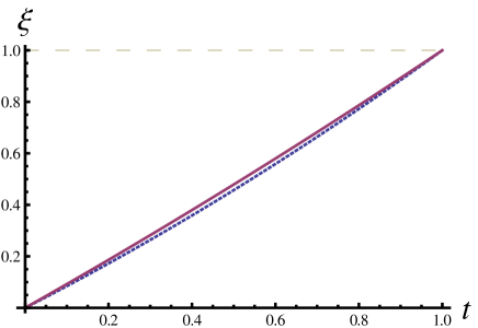
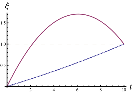
Figure 1: Optimal trajectory between position $x_{0}=0$ and and $x_{\tau}=1$ as a function of time for $T_{0}=1$, $\vartheta=1$, $\gamma_{0}=1$. The dotted line refers to the case without the entropic anomaly and the solid line to the anomalous case of inhomogeneous temperature, while the reference dashed line indicates the arrival position $x_{\tau}$. Top: transport in a time $\tau=1$. Bottom: transport in a time $\tau=10$.

Since (17) (like its general counterpart (16)) is obtained from extremizing a “Lagrange-function” (9), we actually face a Hamiltonian dynamics with preserved “energy” $(D^{-1})_{ij}\dot{\xi}^{i}\dot{\xi}^{j}+U$. Therefore, (17) can be easily solved for the quadratic velocity with the result

$$\dot{\xi}\dot{\xi} = \left(C-U(\xi)\right)D(\xi)$$ (18)

$$= CD(\xi)+\frac{1}{2\gamma^{2}(\xi)}\left(\frac{dT(\xi)}{d\xi}\right)^{2}\,,$$

where $C$ is an integration constant corresponding to the conserved “energy”. For the thermally inhomogeneous study case we choose a linear temperature profile and a constant friction coefficient

$$T(x)=T_{0}+\vartheta x\,,\qquad\gamma=\gamma_{0}\,,$$ (19)

with constant temperature gradient $\vartheta$. In order to avoid non-physical zero or negative temperatures we restrict to positions larger than $x_{\mathrm{min}}=-T_{0}/\vartheta$. For the case of space-dependent friction we can define

$$T=T_{0}\,,\qquad\gamma(x)=\frac{\gamma_{0}}{1+\vartheta/T_{0}\,x}\,.$$ (20)

Therefore, in both cases, we have the same space dependent diffusion coefficient

$$D(x)=\frac{T_{0}+\vartheta x}{\gamma_{0}}\,,$$ (21)

but only for the space-dependent temperature profile the second term in (18) contributes, representing the anomalous entropy production. With these definitions, the right-hand side of (18) is linear in $\xi$ and can be solved explicitly with a solution that is quadratic in time:

$$\xi(t;x_{0})=x_{0}-\bigl{(}x_{0}+X\bigr{)}\frac{t}{\tau}+\bigl{(}x_{\tau}+X\bigr{)}\left(\frac{t}{\tau}\right)^{2}$$ (22)

with

$$X=x_{0}+\frac{2T_{0}}{\vartheta}-\sqrt{4\left(x_{0}+\frac{T_{0}}{\vartheta}\right)\left(x_{\tau}+\frac{T_{0}}{\vartheta}\right)+\chi\frac{\vartheta^{2}\tau^{2}}{2\gamma_{0}^{2}}}\,,$$ (23)

and the prescribed initial position $\xi(0;x_{0})=x_{0}$ and final position $\xi(\tau;x_{0})=x_{\tau}$, where for the sake of simplicity we have considered $x_{\tau}>x_{0}$ (i.e. motion towards the hotter region). In (23), we have introduced the characteristic parameter $\chi$ to distinguish between the anomalous case with inhomogeneous temperature (setup (19), $\chi=1$) and the regular one with constant temperature but space-dependent friction (setup (20), $\chi=0$). Actually, the term involving $\chi$ in the square root represents $-\tau^{2}DU$ coming from (18).

Beside its dependence on the parameters that define the specific system (like $T_{0}$, $\vartheta$, and $\gamma_{0}$), and on the initial and final positions $x_{0}$, $x_{\tau}$, this optimal solution also depends on the process duration $\tau$. In the absence of the anomalous contribution to the entropy production ($\chi=0$), this dependence corresponds to a trivial rescaling of time. The optimal trajectory then is a parabola with positive curvature $x_{\tau}+X|_{\chi=0}$, independent of process duration. In presence of the anomaly ($\chi=1$), however, the evolution of $\xi(t;x_{0})$ depends on $\tau$ also via $X$ and can change qualitatively. For processes that take exactly $\tau=\sqrt{2}(x_{\tau}-x_{0})\gamma_{0}/\vartheta$, the solution $\xi(t;x_{0})$ is a straight line, while it is a parabola with a positive (negative) concavity for shorter (longer) process durations. Interestingly, for very slow processes with

$$\tau>\tau_{\mathrm{o.s.}}=\frac{2\gamma_{0}}{\vartheta}\sqrt{2(x_{\tau}-x_{0})(x_{\tau}+\frac{T_{0}}{\vartheta})}$$ (24)

the optimal trajectory even overshoots the target position at $x_{\tau}$ and eventually changes direction to finally reach it. Such a counter-intuitive behavior can be traced back to the influence of the anomalous contribution to the “cost” of the optimal trajectory.

In the present case, the entropic cost of the optimal evolution reads (see eqs. (9), (10), (14) and (18))

$$S_{\xi} = \int_{0}^{\tau}\mathrm{d}t\,\left[C-2U(\xi)\right]$$ (25)

$$= \int_{0}^{\tau}\mathrm{d}t\,\left[\frac{4\gamma_{0}}{\vartheta\tau^{2}}\bigl{(}x_{\tau}+X\bigr{)}+\chi\frac{\vartheta^{2}/\gamma_{0}}{T_{0}+\vartheta\xi}\right]\,,$$

where in the second step we have used the explicit form (19) of the linear temperature profile. The first term of the integrand of the cost is constant whereas the second one depends on the position $\xi$. In fact, the instantaneous cost is lower at high temperatures which, in this case, are reached for large values of $\xi$. When the transport time is fixed and long it can therefore be profitable to spend part of it where the anomalous term is less costly even though this is away from the target.

It is now interesting to consider the dependence of the total cost on the duration of the transport operation $\tau$ (Fig. 2).

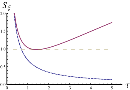
Figure 2: Optimal cost between position $x_{0}=0$ and and $x_{\tau}=1$ as a function of process duration $\tau$ for $T_{0}=1$, $\vartheta=1$, $\gamma_{0}=1$. The dotted line refers to the case without the entropic anomaly (solved by geodesics) and the solid line to the anomalous case of inhomogeneous temperature. The reference dashed line indicates the minimum cost for the anomalous case achieved for a time $\tau=\frac{\sqrt{2}(x_{\tau}-x_{0})\gamma_{0}}{\vartheta}=\sqrt{2}$.

Naively we would expect a slow, quasi-static process (long $\tau$) to be less dissipative and therefore associated with a lower entropy production. For the non-anomalous setting of constant temperature this is indeed the case (see [12]) as we have

$$S_{\xi}(\tau)=\frac{4\gamma_{0}}{\vartheta\tau}\bigl{(}x_{\tau}+X|_{\chi=0}\bigr{)}\sim\frac{1}{\tau}\,.$$ (26)

When a temperature gradient is present the situation changes drastically as the anomalous contribution increases with the process duration and the minimum cost is achieved at finite time. For the discussed linear temperature profile the optimal cost reads

$$S_{\xi}(\tau) = \frac{4\gamma_{0}}{\vartheta\tau}\left(x_{\tau}+X|_{\chi=1}\right)$$ (27)

$$+ \sqrt{2}\log{\left[\frac{1-\left(\frac{x_{\tau}+X|_{\chi=1}-\frac{\vartheta\tau}{\gamma_{0}\sqrt{2}}}{x_{\tau}-x_{0}}\right)^{2}}{1-\left(\frac{x_{\tau}+X|_{\chi=1}+\frac{\vartheta\tau}{\gamma_{0}\sqrt{2}}}{x_{\tau}-x_{0}}\right)^{2}}\right]}$$

where we recall that $X|_{\chi=1}$ also depends on $\tau$ as specified in (23). This expression is not a monotonic decreasing function of $\tau$ and therefore, there is a finite valued $\tau$ minimizing it:

$$\tau^{*}=\frac{\sqrt{2}(x_{\tau}-x_{0})\gamma_{0}}{\vartheta}\,.$$ (28)

It is interesting to note that this optimal duration of the protocol depends inversely on the intensity of the gradient and corresponds to the case in which the solution of (22) is a straight line. Furthermore, considering (24), we can see that the overshooting of the final target takes places for transport times that are longer than the optimal ones $\tau_{\mathrm{o.s.}}=2\sqrt{\frac{x_{\tau}+T_{0}/\vartheta}{(x_{\tau}-x_{0})}}\tau^{*}>2\tau^{*}$. Before moving to the conclusion we wish to recall that, although the solutions (22) are sufficient to assess the optimal transport duration and highlight several peculiarities of the optimal protocol in presence of temperature gradients, they still depend on the explicit evolution of the probability density (via the current velocity). In order to have a complete solution for the protocols one has to consider the specific initial distribution and solve the corresponding assignment problem.

5 Conclusion

We have shown that the optimization of entropy production for driven diffusion processes in an inhomogeneous temperature environment can be mapped into an auxiliary deterministic transport problem describing motion on a curved manifold. The metric tensor of the manifold is given by the inverse of the diffusion matrix. Contributions to the entropy production due to the “entropic anomaly” [18] play the role of a potential energy for the auxiliary deterministic dynamics on the curved manifold. In non-anomalous cases the optimization reduces to the solution of geodesics. Recently, geodesics were found as optimal solutions in control parameter space for excess power in [14] within a linear response analysis, and for slowly varying protocols driving a particle in a harmonic potential in [17]. Using the simple example of one-dimensional diffusion in a linear temperature gradient, we demonstrated that optimization of entropy production including the anomaly requires finite processing times which are inversely proportional to the gradient. In contrast, for regular settings (homogeneous temperature), the optimal average entropy production is reached in the quasi-static limit of adiabatically slow operation. We have also shown that for slow transports the anomalous optimal trajectory is markedly different from the regular one and may display non trivial features such as overshooting of the final target. We have here presented the details in the case of a space-dependent temperature and friction coefficient. However, temperature and viscosity (friction) variations with time can be treated along similar lines, the main difference to our central result (16) being an additional term from the time-derivative of the metric tensor.

- [1] \NameBlickle V. Bechinger C. \REVIEWNat. Phys.82012143.
- [2] \NameBérut A., Arakelyan A., Petrosyan A., Ciliberto S., Dillenschneider R. Lutz E. \REVIEWNature4832012187.
- [3] \NameSekimoto K. \BookStochastic Energetics \Vol799 \PublLecture Notes in Physics, Springer, Berlin Heidelberg \Year2010.
- [4] \NameSeifert U. \REVIEWRep. Prog. Phys.7520121.
- [5] \NameJarzynski C. \REVIEWPhys. Rev. Lett.7819972690.
- [6] \NameSchmiedl T. Seifert U. \REVIEWPhys. Rev. Lett.982007108301.
- [7] \NameSchmiedl T. Seifert U. \REVIEWEPL812008 20003.
- [8] \NameThen H. Engel A. \REVIEWPhys. Rev. E772008041105.
- [9] \NameGeiger P. Dellago C. \REVIEWPhys. Rev. E812010021127.
- [10] \NameAurell E., Mejia-Monasterio C. Muratore-Ginanneschi P. \REVIEWPhys. Rev. Lett.1062011250601.
- [11] \NameAurell E., Mejia-Monasterio C. Muratore-Ginanneschi P. \REVIEWPhys. Rev. E852012020103(R).
- [12] \NameAurell E., Gawȩdzki K., Mejia-Monasterio C., Mohayaee R. Muratore-Ginanneschi P. \REVIEWJ. Stat. Phys.1472012487.
- [13] \NameMuratore-Ginanneschi P. \ReviewarXiv:1210.1133 [cond-mat.stat-mech]\Year2012.
- [14] \NameSivak D. A.Crooks G. E. \REVIEWPhys. Rev. Lett.1082012190602.
- [15] \NameJülicher F., Ajdari A. Prost J. \REVIEWRev. Mod. Phys 6919971269–1282.
- [16] \NameReimann P. \REVIEWPhys. Rep.361200257.
- [17] \NameZulkowski P. R., Sivak D. A., Crooks G. E. DeWeese M. R. \REVIEWPhys. Rev. E862012041148
- [18] \NameCelani A., Bo S., Eichhorn R. Aurell E. \REVIEWPhys. Rev. Lett.1092012260603.
- [19] \NameLau A. W. C. Lubensky T. C \REVIEWPhys. Rev. E762007011123
- [20] See the Supplementary Information of [18].
- [21] \NameChetrite R. Gawȩdzki K. \REVIEWCommun. Math. Phys.2822007469.
- [22] \NameSeifert U. \REVIEWPhys. Rev. Lett.952005040602.
- [23] \NameNelson E. \BookDynamical theories of Brownian motion \PublPrinceton University Press, Princeton N. J. \Year1967
- [24] \NameGuerra F.Morato L. M. \REVIEWPhys. Rev. D2719831774.