Spread of visited sites of a random walk along the generations of a branching process

Abstract

In this paper we consider a null recurrent random walk in random environment on a super-critical Galton-Watson tree. We consider the case where the log-Laplace transform $\psi$ of the branching process satisfies $\psi(1)=\psi^{\prime}(1)=0$ for which G. Faraud, Y. Hu and Z. Shi in [9] show that, with probability one, the largest generation visited by the walk, until the instant $n$, is of the order of $(\log n)^{3}$. In [3] we prove that the largest generation entirely visited behaves almost surely like $\log n$ up to a constant. Here we study how the walk visits the generations $\ell=(\log n)^{1+\zeta}$, with $0<\zeta<2$. We obtain results in probability giving the asymptotic logarithmic behavior of the number of visited sites at a given generation. We prove that there is a phase transition at generation $(\log n)^{2}$ for the mean of visited sites until $n$ returns to the root. Also we show that the visited sites spread all over the tree until generation $\ell$.

1 Introduction

We start giving an iterative construction of the environment. Let $(A_{i},i\geq 1)$ a positive random sequence and $N$ an independent $\mathbb{N}$-valued random variable following a distribution $q$, in other words $\mathbb{P}(N=i)=q_{i}$ for $i\in\mathbb{N}$. Let $\phi$ the root of the tree and $(A(\phi^{i}),i\leq N_{\phi}))$ an independent copy of $(A_{i},i\leq N)$. Then, we draw $N_{\phi}$ children to $\phi$: these individuals are the first generation. Each child $\phi_{i}$ is associated with the corresponding $A(\phi^{i})$ and so on. At the $n$-th generation, for each individual $x$ we pick $(A(x^{i}),i\leq N_{x})$ an independent copy of $(A_{i},i\leq N)$ where $N_{x}$ is the number of children of $x$ and $A(x^{i})$ is the random variable attached to $x^{i}$. The set $\mathbb{T}$, consisting of the root and its descendants, forms a Galton-Watson tree (GW) of offspring distribution $q$ and where each vertex $x\neq\phi$ is associated with a random variable $A(x)$.
We denote by $|x|$ the generation of $x$, $\overset{\leftarrow}{x}$ the parent of $x$, and for convenience reasons we add $\overset{\leftarrow}{\phi}$, the parent of $\phi$. The set of environments denoted by E is the set of all sequences $((A(x^{i}),i\leq N_{x}),x\in\mathbb{T})$, with $P$ and $E$ respectively the associated probability measure and expectation.
We assume that the distribution of $(A_{i},i\leq N)$ is non-degenerate and, to obtain a supercritical GW, that $E[N]>1$. Moreover we add uniform ellipticity conditions

$$\exists\ 0<\varepsilon_{0}<1,\ P-a.s\ \ \forall i,\varepsilon_{0}\leq A_{i}\leq 1/\varepsilon_{0},$$ (1.1)

$$\exists\ N_{0}\in\mathbb{N},P-a.s\ N\leq N_{0}.$$ (1.2)

Given $\mathcal{E}\in\bf E$, we define a $\mathbb{T}$-valued random walk $(X_{n})_{n\in\mathbb{N}}$ starting from $\phi$ by its transition probabilities,

$$p(x,x^{i})=\frac{A(x^{i})}{\sum_{j=1}^{N_{x}}A(x^{j})+1},\ p(x,\overset{\leftarrow}{x})=1-\sum_{j=1}^{N_{x}}p(x,x^{j}),\ p(\overset{\leftarrow}{\phi},\phi)=1.$$

Note that our construction implies that $(p(x,.),x\in\mathbb{T})$ is an independent sequence. We denote by $\mathbb{P}^{\mathcal{E}}$ the probability measure associated to this walk, the whole system is described under the probability $\mathbb{P}$, the semi-direct product of $P$ and $\mathbb{P}^{\mathcal{E}}$.
To study asymptotical behaviours associated to $(X_{n})_{n\in\mathbb{N}}$, a quantity appears naturally: the potential process $V$ associated to the environment which is actually a branching random walk. It is defined by $V(\phi):=0$ and

$$V(x):=-\sum_{z\in\rrbracket\phi,x\rrbracket}\log A(z),x\in\mathbb{T}\backslash\{\phi\},$$

where $\llbracket\phi,x\rrbracket$ is the set of vertices on the shortest path connecting $\phi$ to $x$ and $\rrbracket\phi,x\rrbracket=\llbracket\phi,x\rrbracket\backslash\{\phi\}$. We put ourself in the non lattice case so $\log A_{i}$ can not be written as $b+c\mathbb{Z}$, and introduce the moment-generating function

$$\psi(t):=\log E\left[\sum_{|x|=1}e^{-tV(x)}\right],$$

characterizing the environment. Note that the hypothesis we discuss above implies that $\psi$ is defined on $\mathbb{R}$, and $\psi(0)>0$. In fact the hypothesis (1.1) and $\eqref{hyp2}$ are not always needed for our work and they could be replaced by the existence of $\psi$ in $(-\delta,1+\delta)$ with $\delta>0$ together with the existence of a moment larger than 1 for $N$. In Section 2 for example we could lighten the hypothesis this way, but it would be much more complicated in Section 4.
Thanks to the work of M.V. Menshikov and D. Petritis, see [15] and the first part of [8] by G. Faraud, if

$$\psi(1)=\psi^{\prime}(1)=0$$ (1.3)

then $X$ is null recurrent, with $\psi^{\prime}(1)=-E\left[\sum_{|x|=1}V(x)e^{-V(x)}\right]$. In [9] (see also [12]), G. Faraud, Y. Hu and Z. Shi study the asymptotic behavior of $\max_{0\leq i\leq n}{|X_{i}|}=X_{n}^{*}$, i.e. the largest generation visited by the walk. Assuming (1.3), they prove the existence of a positive constant $a_{0}$ (explicitely known) such that $\mathbb{P}$ a.s. on the set of non-extinction of the GW

$$\lim_{n\rightarrow+\infty}\frac{X_{n}^{*}}{(\log n)^{3}}=a_{0}.$$ (1.4)

In [3] we were interested in the largest generation entirely visited by the walk, that is to say the behavior of $R_{n}:=\sup\{k\geq 1,\forall|z|=k,\mathcal{L}(z,n)\geq 1\}$, with $\mathcal{L}$ the local time of $X$ defined by $\mathcal{L}(z,n):=\sum_{k=1}^{n}\mathds{1}_{X_{k}=z}$. More precisely, if (1.3) is realized, $\mathbb{P}$ a.s. on the set of non-extinction

$$\lim_{n\rightarrow+\infty}\frac{R_{n}}{\log n}=\frac{1}{\tilde{\gamma}},$$ (1.5)

where $\tilde{\gamma}:=\sup\{a\in\mathbb{R},\ \tilde{J}(a)>0\}$ with $\tilde{J}(a):=\inf_{t\geq 0}\{\psi(-t)-at\}$.
Although in [3] all recurrent cases are treated, here we focus only on the hypothesis $\eqref{hyp0}$.
According to (1.4) and (1.5), until generation $\nicefrac{{\log n}}{{\tilde{\gamma}}}$ all the points are visited but $X$ does not visit generations further than $a_{0}(\log n)^{3}$. The aim of this paper is to study the asymptotic of the number of visited sites at a given generation $(\log n)^{1+\zeta}$ with $0<\zeta<2$. For this purpose we define the number of visited sites at generation $m\in\mathbb{N}$ until the instant $n$

$$M_{n}(m):=\#\{|z|=m,\mathcal{L}(z,n)\geq 1\},$$

and before $n$ returns to the root $K_{n}(.):=M_{T_{\phi}^{n}}(.)$ where $T_{x}^{n}=\inf\{k>T_{x}^{n-1},X_{k}=x\}$ for $n\geq 1$ and $T_{x}^{0}=0$ for $x\in\mathbb{T}$.
Let $Z_{m}$ the number of descendants at generation $m\in\mathbb{N}$, we have $Z_{1}=N$. Our first results quantify the number of visited points at a given generation $\ell:=(\log n)^{1+\zeta}$. Thanks to the hypothesis of ellipticity, $\psi$ can be written as a power series in particular, for any $x$ small enough, $\psi(1-x)=\sum_{j=1}^{+\infty}u_{j}x^{j}$, where $u_{j}=\psi^{(j)}(1)$, these are called cumulants and here $u_{1}:=\psi^{\prime}(1)=0$, $u_{2}:=\psi^{\prime\prime}(1)=\sigma^{2}$. Let us define the function $f$, for any $x$ small enough

$$f(x):=1-\frac{x}{2\sigma^{2}}+x^{2}\lambda(x).$$

$\lambda$ is the Cramér’s series depending on the cumulants of $\psi(1-x)$ (for more details on the Cramér’s series see for example [17] p. 219-223).

Theorem 1.1

For all $0<\zeta<2$, $\varepsilon>0$ independent of $\zeta$ there exists $C_{0}>0$ such that

$$\lim_{n\rightarrow+\infty}\mathbb{P}\left(\frac{\psi(0)}{\tilde{\gamma}}(1-\varepsilon)\leq\frac{\log M_{n}(\ell)}{\log n}\leq 1-C_{0}\left(\frac{\log\log n}{\log n}\vee\frac{1}{(\log n)^{\zeta}}\right)\right)=1.$$ (1.6)

Also for all $n$ large enough, there exist two positive constants $C_{1}$ and $C_{2}$ such that

$$\frac{C_{1}}{(\log n)^{\varepsilon}}\frac{e^{(\log n)\cdot f[(\log n)^{-\zeta}]}}{(\log n)^{(1+\tilde{\zeta})/2}}\leq{\mathbb{E}[K_{n}(\ell)]}\leq C_{2}\frac{e^{(\log n)\cdot f[(\log n)^{-\zeta}]}}{(\log n)^{(1+\tilde{\zeta})/2}},$$ (1.7)

with $\tilde{\zeta}:=\mathds{1}_{0<\zeta<1}+\zeta\mathds{1}_{1\leq\zeta<2}$.

(1.6) shows that, at each generation $\ell$, the cardinal of visited sites is at least $n^{\psi(0)(1-\varepsilon)/\tilde{\gamma}}$ for any $\zeta$, that is to say like the last generation entirely visited $R_{n}$ ($\psi(0)/\tilde{\gamma}<1$, by convexity of $\psi$ and the fact that $\psi(1)=0$). Also the upper bound of $M_{n}(\ell)$ is at most of the order of $ne^{-C_{3}(\log n)^{1-\zeta}}/(\log n)^{C_{4}}$, with $C_{3},C_{4}>0$. This suggests that it may have a phase transition when $\zeta=1$. Although we are not able to show this for $M_{n}(\ell)$ the existence of a phase transition is proved in (1.7) for the mean of $K_{n}(\ell)$. Indeed by definition of $f$,

$$(\log n)f[(\log n)^{-\zeta}]=\log n-\frac{(\log n)^{1-\zeta}}{2\sigma^{2}}+(\log n)^{1-2\zeta}\lambda((\log n)^{-\zeta})$$

We can see that in the neighborhood of generation $(\log n)^{2}$ that is to say when $\zeta=1$, the asymptotic behavior of $\mathcal{N}_{\zeta}:=\mathbb{E}[K_{n}(\ell)]$ changes. We easily check that for all $0<\zeta<\zeta^{\prime}\leq 1$, $\lim_{n\rightarrow+\infty}\mathcal{N}_{\zeta^{\prime}}/\mathcal{N}_{\zeta}=+\infty$ whereas for all $1\leq\zeta<\zeta^{\prime}<2$, $\lim_{n\rightarrow+\infty}\mathcal{N}_{\zeta^{\prime}}/\mathcal{N}_{\zeta}=0$. So the generations of order $(\log n)^{2}$ are, in mean, the most visited generation (in term of distinct site visited) until $n$ returns to the origin. Finally notice that when $\zeta>1/2$ we are in a Gaussian behavior as $e^{(\log n)f[(\log n)^{-\zeta}]}\sim ne^{-\frac{(\log n)^{1-\zeta}}{2\sigma^{2}}}$, and when $\zeta\geq 1$, $e^{(\log n)f[(\log n)^{-\zeta}]}\sim n$.

In order to establish our second result, recall Neveu’s notation to introduce a partial order on our tree. In [16], to each vertex $x$ at generation $m\in\mathbb{N}$, Neveu associates a sequence $x_{1}\dots x_{m}$ where $x_{i}\in\mathbb{N}$, to simplify we write $x=x_{1}\dots x_{m}$.
This sequence gives the complete “genealogy” of $x$: if $y=x_{1}\dots x_{i}$ with $|y|=i<m$, $y$ is the unique ancestor of $x$ at generation $i$ and we write $y<x$.
For instance $\overset{\leftarrow}{x}=x_{1}\dots x_{m-1}$ and $1\leq x_{m}\leq N_{\overset{\leftarrow}{x}}$, in other words $x$ is the $x_{m}$-th child of $\overset{\leftarrow}{x}$.
To extend this partial order for $|x|=|z|$, we write $x<z$ if there exists $i<m$ such that $x_{k}=z_{k}$ for $k<i$ and $x_{i}<z_{i}$. Hence we can number individuals at a given generation “from the left to the right” and for $A$ a subset of $\{z\in\mathbb{T},|z|=m\}$, ${\bf inf}\,A$ and ${\bf sup}\,A$ are respectively the minimum and maximum associated to this numbering.
Our last result gives an idea of the way the visited points spread on the tree, for this purpose we introduce clusters: let $z\in\mathbb{T}$ and $m\geq|z|$, we call cluster issued from $z$ at generation $m$ denoted $\mathcal{C}_{m}(z)$, the set of descendants $u$ of $z$ such that $|u|=m$, in other words

$$\mathcal{C}_{m}(z):=\{u>z,\ |u|=m\}.$$ (1.8)

At some point we need to quantify the number of individuals between two disjoint clusters with common generations. For given initial and terminal generations, denote $\mathscr{C}$ a set of disjoint clusters. Let $(\mathcal{D}_{j},1\leq j\leq|\mathscr{C}|)$, with $|\mathscr{C}|$ the cardinal of $\mathscr{C}$, an ordered sequence of (disjoint) clusters belonging to $\mathscr{C}$, that is to say for all $j$, ${\bf sup}\,\mathcal{D}_{j}<{\bf inf}\,\mathcal{D}_{j+1}$. We define the minimal distance between clusters in the following way ${\bf{D}}(\mathscr{C}):=\min_{1\leq j\leq|\mathscr{C}|-2}({\bf inf}\,\mathcal{D}_{j+2}-{\bf sup}\,\mathcal{D}_{j})$, where, by definition, ${\bf inf}\,\mathcal{D}_{j+2}-{\bf sup}\ \mathcal{D}_{j}$ is the number of individuals between ${\bf sup}\,\mathcal{D}_{j}$ and ${\bf inf}\,\mathcal{D}_{j+2}$. Notice that we do not look at two successive clusters, but two successive separate by one. We now state a second result

Theorem 1.2

For $0<\zeta<2$ and $\varepsilon>0$ recalling that $\ell=(\log n)^{1+\zeta}$

$$\lim_{n\rightarrow+\infty}\mathbb{P}\left(\max_{|z|=\ell-\log n/\tilde{\gamma}}\min_{y\in\mathcal{C}_{\ell}(z)}{\mathcal{L}(y,n)\geq 1}\right)=1,$$ (1.9)

$$\lim_{n\rightarrow+\infty}\mathbb{P}\left(\min_{z\in\mathcal{C}_{\varepsilon\ell^{1/3}}(\phi)}\max_{y>z,|y|=\ell}\mathcal{L}(y,n)\geq 1\right)=1.$$ (1.10)

Let $k_{n}$, $h_{n}$ and $r_{n}$ positive sequences of integers such that $k_{n}r_{n}+(k_{n}-1)h_{n}=\ell$. For all $1\leq i\leq k_{n}$, let us denote $\mathscr{C}_{i}$ a set of clusters initiated at generation $(i-1)(r_{n}+h_{n})$ and with end points at generation $ir_{n}+(i-1)h_{n}$ (see Figure 3), also define the following event for all $m>0$ and $q>0$

$$\mathscr{A}_{i}(m,q):=\bigcup_{\mathscr{C}_{i}}\left\{\left\{{|\mathscr{C}_{i}|\geq q,\bf{D}}(\mathscr{C}_{i})\geq m\right\}\bigcap_{\mathcal{D}\in\mathscr{C}_{i}}\left\{{\forall z\in\mathcal{D},\mathcal{L}(z,n)\geq 1}\right\}\right\}.$$

There exist $0<{\bf k}<1\wedge\zeta$, $0<{\bf r}<1$ with $0<{\bf k}+{\bf r}\leq 1$ and for $k_{n}=(\log n)^{{\bf k}}$, $r_{n}=(\log n)^{{\bf r}}$

$$\lim_{n\rightarrow+\infty}\mathbb{P}\left(\bigcap_{i=2}^{k_{n}}\mathscr{A}_{i}(e^{\psi(0)h_{n}/2},e^{\psi(0)r_{n}(i-1)/2})\right)=1.$$ (1.11)

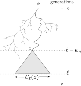
Figure 1: One large cluster

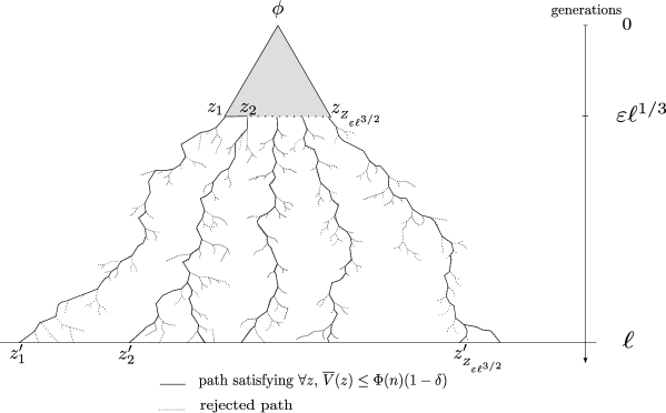
Figure 4: Distant visited sites

(1.9) implies the existence of a cluster starting at a generation $\ell-\log n/\tilde{\gamma}$ completely visited (see Figure 1). As conditionnaly on the tree until generation $|z|$, $|\mathcal{C}_{\ell}(z)|$ is equal in law to $Z_{\ell-|z|}=Z_{\psi(0)\log n/\tilde{\gamma}}$, this cluster is large and, in particular, (1.9) implies the lower bound in (1.6).
(1.10) tells that we can find visited individuals at generation $\ell=(\log n)^{1+\zeta}$, with a common ancestor to a generation close to the root, that is to say before generation $\varepsilon\ell^{1/3}$ (see Figure 4). Thus, with a probability close to one, at least $e^{\varepsilon(1-\varepsilon)\psi(0)\ell^{1/3}/2}$ individuals of generation $\ell$ separate by at least $e^{\psi(0)\ell/2}$ individuals of the same generation $\ell$, are visited.
Finally (1.11) tells that if we make cuts regularly on the tree we can find many visited clusters (which number increases with the generation) well separated. In particular these visited clusters can not be in a same large visited clusters as they are separated by at least $e^{\psi(0)h_{n}/2}\sim e^{\psi(0)(\log n)^{1+\zeta-\bf{k}}/2}>n$ individuals (see also Figure 3).

To obtain these results we show that $K_{n}(\ell)$ can be linked to a random variable depending only on the random environment and $n$. For all $z\in\mathbb{T}$, all integer $k$ and all real $a$, we define the random variable

$$\mathcal{R}_{a}^{z}(k):=\#\{u>z,|u|=k,\overline{V}(z)\leq a\},$$

where $\overline{V}(z)=\max_{u\in\rrbracket\phi,z\rrbracket}V(u)$. For notational simplicity, we write $\mathcal{R}_{a}(k)$ for $\mathcal{R}_{a}^{\phi}(k)$. We obtain the following

Proposition 1.3

Let $\varepsilon>0$ and $\Phi$ a sequence such that

$$(1-\varepsilon)\log n\leq\Phi(n)\leq\log n+o(\log n).$$ (1.12)

Then, for all $0<\zeta<2$ there exists $C_{0}^{\prime}>0$

$$\lim_{n\rightarrow+\infty}P\left(\frac{\psi(0)}{\tilde{\gamma}}(1-\varepsilon)\leq\frac{\log\mathcal{R}_{\Phi(n)}(\ell)}{\Phi(n)}\leq 1-C_{0}^{\prime}\left(\frac{\log\log n}{\Phi(n)}\vee\frac{\Phi(n)}{\ell}\right)\right)=1,$$ (1.13)

$$E[\mathcal{R}_{\Phi(n)}(\ell)]\asymp(\ell^{-1}\mathds{1}_{0<\zeta<1}+\Phi(n){\ell^{-3/2}}\mathds{1}_{1\leq\zeta<2}){e^{\Phi(n)f(\Phi(n)/\ell)}}.$$ (1.14)

We use the notation $a_{n}\asymp b_{n}$ when there exists two positive constants $c_{1}$ and $c_{2}$ such that $c_{1}b_{n}\leq a_{n}\leq c_{2}b_{n}$ for all $n$ large enough. The lack of precision for the first result shows no difference between $\mathcal{R}_{\log n}(\ell)$ and $M_{n}(\ell)$ (see (1.6)), unlike between the means of $\mathcal{R}_{\log n}(\ell)$ and ${K}_{n}(\ell)$.

The rest of the paper is organized as follow: in Section 2 we study $\mathcal{R}_{\Phi(n)}(\ell)$ and prove Proposition 1.3. In Section 3 we link $\mathcal{R}_{\Phi(n)}(\ell)$ and $M_{n}(\ell)$, which leads to Theorem 1.1 and (1.9) of Theorem 1.2. In Section 4 we prove the end of Theorem 1.2. Also we add an appendix where we state known results on branching processes and local limit theorems for sums of i.i.d. random variables.
Note that for typographical simplicity, we do not distinguish a real number and its integer part throughout the article.

2 Expectation and bounds of $\boldsymbol{\mathcal{R}_{\Phi(n)}(\ell)}$

In this section we only work with the environment more especially with what we call number of accessible points $\mathcal{R}_{\Phi(n)}(\ell)$.

2.1 Expectation of $\boldsymbol{\mathcal{R}_{\Phi(n)}(\ell)}$ (proof of (1.14))

According to Biggins-Kyprianou identity (also called many-to-one formula, see part A of appendix), $E[\mathcal{R}_{\Phi(n)}(\ell)]=E\left[e^{S_{\ell}}\mathds{1}_{\bar{S}_{\ell}\leq\Phi(n)}\right]$ where $S_{j}$ is a centered random walk, we only have to prove

Lemma 2.1

For all $\varepsilon>0$, $\Phi$ satisfying (1.12), for all $0<\zeta<2$

$$E\left[e^{S_{\ell}}\mathds{1}_{\bar{S}_{\ell}\leq\Phi(n)}\right]\asymp e^{\Phi(n)f(\Phi(n)/\ell)}\left[\ell^{-1}\mathds{1}_{0<\zeta\leq 1}+\Phi(n)\ell^{-3/2}\mathds{1}_{1\leq\zeta<2}\right].$$

Proof.
For $\varepsilon>0$:

$$E\left[e^{S_{\ell}}\mathds{1}_{\bar{S}_{\ell}\in{\bf I}_{\Phi(n)}}\right]\leq E\left[e^{S_{\ell}}\mathds{1}_{\bar{S}_{\ell}\leq\Phi(n)}\right]\leq E\left[e^{S_{\ell}}\mathds{1}_{\bar{S}_{\ell}\in{\bf I}_{\Phi(n)}}\right]+e^{\Phi(n)(1-\varepsilon)}.$$

with $I_{\Phi}:=]\Phi(n)(1-\varepsilon),\Phi(n)]$. For every sequence $(u_{n})_{n\in\mathbb{N}}$, we denote $\bar{u}_{j}:=\max_{1\leq i\leq j}u_{i}$ and $\underline{u}_{j}:=\min_{1\leq i\leq j}u_{i}$, also let $\mathscr{S}_{j}:=\{\bar{S}_{j-1}<S_{j}=\bar{S}_{\ell}\}$. First, as $S_{0}=0$

$$\sum_{j=1}^{\ell}E\left[e^{S_{\ell}}\mathds{1}_{{S}_{j}\in{\bf I}_{\Phi(n)},\mathscr{S}_{j}}\right]\leq E\left[e^{S_{\ell}}\mathds{1}_{\bar{S}_{\ell}\in{\bf I}_{\Phi(n)}}\right]\leq\sum_{j=1}^{\ell}E\left[e^{S_{\ell}}\mathds{1}_{{S}_{j}\in{\bf I}_{\Phi(n)},\mathscr{S}_{j}}\right]+1.$$

For $0\leq i\leq j$, let $\tilde{S}_{i}:=S_{j}-S_{j-i}$, with this notation $\{\bar{S}_{j-1}<S_{j}\}=\{\tilde{\underline{S}}_{j-1}>0\}$ and $\tilde{S}_{j}=S_{j}$. Writing $S$ as a sum of i.i.d. random variables, we easily see that $(S_{i})_{0\leq i\leq j}$ and $(\tilde{S}_{i})_{0\leq i\leq j}$ have the same law. Then, conditioning on $\sigma\{S_{k},k\leq j\}$

$$E\left[e^{S_{\ell}}\mathds{1}_{{S}_{j}\in{\bf I}_{\Phi(n)},\mathscr{S}_{j}}\right]=D_{j}F_{\ell-j}$$ (2.1)

with $F_{m}:=E\left[e^{S_{m}}\mathds{1}_{\bar{S}_{m\leq 0}}\right]$ and $D_{j}:=E\left[e^{S_{j}}\mathds{1}_{S_{j}\in{\bf I}_{\Phi(n)},\underline{S}_{j-1}>0}\right]$.
By (B.1), $\forall j\leq\ell,\,F_{\ell-j}\asymp(\ell-j+1)^{-3/2}$ then it remains to estimate $D_{j}$. For any $A>0$

$$D_{j} =\sum_{k=\Phi(n)(1-\varepsilon)+1}^{\Phi(n)}E\left[e^{S_{j}}\mathds{1}_{k-1<S_{j}\leq k,\underline{S}_{j}>0}\right]$$

$$\asymp\sum_{k=\Phi(n)(1-\varepsilon)+1}^{\Phi(n)}e^{k}P(k-1<S_{j}\leq k,\underline{S}_{j}>0)(\mathds{1}_{k\leq Aj^{1/2}}+\mathds{1}_{k>Aj^{1/2}})$$

$$=:D_{j}^{1}+D^{2}_{j}.$$

We now need to distinguish the cases $0<\zeta<1$ and $1\leq\zeta<2$.
When $0<\zeta<1$, $D^{1}_{j}=0$ as $k>A\ell^{1/2}$. Also using Lemma B.6 for $A$ large enough

$$H^{2}_{j} :=\sum_{k=\Phi(n)(1-\varepsilon)+1}^{\Phi(n)}e^{k}P(k-1<S_{j}\leq k,\underline{S}_{j}>0)\mathds{1}_{Aj^{1/2}<k<\varepsilon j}$$

$$\asymp\sum_{k=\Phi(n)(1-\varepsilon)+1}^{\varepsilon j\wedge\Phi(n)}e^{k}P(k-1<S_{j}\leq k,\underline{S}_{j}>0)\asymp\sum_{k=\Phi(n)(1-\varepsilon)+1}^{\varepsilon j\wedge\Phi(n)}\frac{e^{kf(k/j)}}{j},$$ (2.2)

recall that $f(x)=1-x/(2\sigma^{2})+x^{2}\lambda(x)$ where $\lambda$ is the Cramér’s serie associated to $V$. (2.2) implies that $H^{2}_{j}\geq c_{-}e^{(\varepsilon j\wedge\Phi(n))f((\varepsilon j\wedge\Phi(n))/j)}/j$. For the upper bound, we can assume without loss of generality that $\varepsilon$ is small enough to ensure that for $|x|\leq\varepsilon$, $\lambda(x)$ converges and $f^{\prime}(x)$ is negative. Therefore, the derivative of $F$ defined by $F(x):=e^{xf(x/j)}/f(x/j)$ satisfies in the same interval $F^{\prime}(x)\geq e^{xf(x/j)}-c_{+}xe^{xf(x/j)}/j\geq e^{xf(x/j)}(1-c_{+}\varepsilon)$, with $c_{+}>0$. Integrating this last inequality, for $\varepsilon$ small enough

$$\int_{\Phi(n)(1-\varepsilon)}^{\varepsilon j\wedge\Phi(n)}e^{xf(x/j)}\leq\left[F(x)\right]_{\Phi(n)(1-\varepsilon)}^{\varepsilon j\wedge\Phi(n)}/(1-c_{+}\varepsilon)\leq C_{+}e^{(\varepsilon j\wedge\Phi(n))f((\varepsilon j\wedge\Phi(n))/j)},$$ (2.3)

and finally

$$H^{2}_{j} \leq\frac{C_{+}}{j}\int_{\Phi(n)(1-\varepsilon)}^{\Phi(n)}e^{xf(x/j)}dx\leq\frac{C_{+}}{j}e^{(\varepsilon j\wedge\Phi(n))f((\varepsilon j\wedge\Phi(n))/j)}.$$

Note that for $s>0$ small enough, $\psi(1-s)\leq{s}/{2}$. So the exponential Markov inequality applied to $P(sS_{j}>sk)$ and the identity $E[e^{sS_{j}}]=e^{j\psi(1-s)}$ yield

$$\tilde{H}^{2}_{j}:=\sum_{k=\Phi(n)(1-\varepsilon)+1}^{\Phi(n)}e^{k}P(k-1<S_{j}\leq k,\underline{S}_{j}>0)\mathds{1}_{k\geq\varepsilon j}\leq e^{\Phi(n)(1-s/2)}.$$

In particular $\tilde{H}^{2}_{j}=o(H_{j}^{2})$ for all $j\geq\Phi(n)^{1+u}$ with $u>0$. Finally, as for any $\varepsilon$ small enough $(\varepsilon j\wedge\Phi(n))f((\varepsilon j\wedge\Phi(n))/j)$ is increasing in $j$, for any $0<u<\zeta$

$$\sum_{j=1}^{\ell}D_{j}F_{\ell-j}\asymp\sum_{j=\Phi(n)^{1+u}}^{\ell}(\ell-j+1)^{-3/2}j^{-1}e^{(\varepsilon j\wedge\Phi(n))f((\varepsilon j\wedge\Phi(n))/j)}\asymp e^{\Phi(n)f(\Phi(n)/\ell)}/\ell.$$ (2.4)

Indeed, writing $\sum_{j=\Phi(n)^{1+u}}^{\ell}(\ell-j+1)^{-3/2}j^{-1}e^{(\varepsilon j\wedge\Phi(n))f((\varepsilon j\wedge\Phi(n))/j)}:=\sum_{j=\Phi(n)^{1+u}}^{\ell}G_{j}$, $\sum_{j=\Phi(n)^{1+u}}^{\ell}G_{j}\geq G_{\ell}$ and as

$$\sum_{j=\Phi(n)^{1+u}}^{\frac{\ell}{2}}G_{j} \leq \frac{C_{+}e^{\Phi(n)f(\Phi(n)/\ell)}}{\phi(n)^{1+u}\ell^{\frac{1}{2}}}\leq\frac{C_{+}e^{\Phi(n)f(\Phi(n)/\ell)}}{\ell},$$

$$\sum_{j=\frac{\ell}{2}+1}^{\ell}G_{j} \leq \frac{C_{+}e^{\Phi(n)f(\Phi(n)/\ell)}}{\ell}\sum_{j=\frac{\ell}{2}+1}^{\ell}{(\ell-j+1)^{-\frac{3}{2}}}\leq\frac{C_{+}e^{\Phi(n)f(\Phi(n)/\ell)}}{\ell},$$

(2.4) follows.
When $1\leq\zeta<2$, we prove that the main contribution comes from $D^{1}_{j}$. As for any $n$ large enough, $\Phi(n)\leq A\ell^{1/2}$ for some $A>0$, for any $j\geq(\Phi(n)/A)^{2}$ using Lemma B.6

$$D^{1}_{j}\asymp\sum_{k=\Phi(n)(1-\varepsilon)}^{\Phi(n)}\frac{ke^{k}}{j^{3/2}}e^{-k^{2}/(2\sigma^{2}j)}\asymp\frac{\Phi(n)}{j^{{3}/{2}}}e^{\Phi(n)f(\Phi(n)/\ell)}.$$

When $j<(\Phi(n)/A)^{2}$, similar computations than for $H_{j}$ and $\tilde{H}_{j}$ give

$$\sum_{j=1}^{\ell}D^{2}_{j}F_{\ell-j} \leq\sum_{j=1}^{(\Phi(n)/A)^{2}}F_{\ell-j}(H_{j}^{2}+\tilde{H}_{j}^{2})\leq C_{+}e^{\Phi(n)(1-(A^{2}/2\sigma^{2}\wedge s/2))}.$$

Finally $\sum_{j=1}^{\ell}D_{j}F_{\ell-j}\asymp{\Phi(n)e^{\Phi(n)f(\Phi(n)/\ell)}}{\ell^{-3/2}},$ this together with (2.4) finishes the proof. $\blacksquare$

2.2 Bounds for $\boldsymbol{\log\mathcal{R}_{\Phi(n)}(\ell)}$ (proof of (1.13))

The upper bound is a direct consequence of Markov inequality and (1.14).
For the lower bound, we first need an estimation on the deviation of $\min_{|z|=m}\overline{V}(m)$, this topic has been studied in details in [9],

Proposition 2.2

Let $a_{n}$ a positive sequence such that $a_{n}\sim n^{1/3}$, there exists $b_{0}>0$ such that for any $0<b<b_{0}$

$$\lim_{n\rightarrow+\infty}\frac{1}{a_{n}}\log P\left(\min_{|z|=n}\overline{V}(z)\leq ba_{n}\right)=b-b_{0}.$$ (2.5)

A useful consequence of the above Proposition is the following

Lemma 2.3

Assume that $a_{n}$ is a positive increasing sequence such that $a_{n}\sim n^{1/3}$, there exists a constant $\mu>0$ such that for any $n$ large enough

$$P\left(\min_{|z|=n}\overline{V}(z)>\mu a_{n}\right)\leq\lambda_{n}+o(\lambda_{n}),$$ (2.6)

where $\lambda_{n}=e^{-c_{1}e^{c_{1}a_{n}}}$ if $q_{0}+q_{1}=0$, and $\lambda_{n}=e^{-{c_{1}a_{n}}}$ otherwise, also $c_{1}>0$ depends only on the distribution $P$.

Proof.
Clearly for $z_{1}<z$, $\overline{V}(z)\leq\overline{V}(z_{1})+\tilde{V}(z_{1},z)$ where $\tilde{V}(z_{1},z)=\max_{z_{1}<x\leq z}V(x)-V(z_{1})$. In the sequel, writing $\tilde{V}(z_{1},z)$ implies that $z_{1}<z$ implicitly. For $0<\eta<1$ and $v_{n}:=\nicefrac{{\eta b_{0}a_{n}}}{{\alpha}}$

$$P\left(\min_{|z|=n}\overline{V}(z)>2\eta b_{0}a_{n}\right)\leq P\left(\min_{|z_{1}|=v_{n}}\min_{|z|=n}\tilde{V}(z_{1},z)>2\eta b_{0}a_{n}-\max_{|z_{1}|=v_{n}}\overline{V}(z_{1})\right).$$

Using that $\max_{|z_{1}|=v_{n}}\overline{V}(z_{1})\leq\alpha v_{n}$ by ellipticity and for $\mathcal{A}_{n}:=\left\{Z_{v_{n}}\geq e^{\eta\psi(0)v_{n}}\right\}$

$$P\left(\min_{|z|=n}\overline{V}(z)>2\eta b_{0}a_{n}\right) \leq P\left(\min_{|z_{1}|=v_{n}}\min_{|z|=n}\tilde{V}(z_{1},z)>\eta b_{0}{a}_{n}\right)$$

$$\leq P\left(\min_{|z_{1}|=v_{n}}\min_{|z|=n}\tilde{V}(z_{1},z)>\eta b_{0}a_{n},\mathcal{A}_{n}\right)+P(\bar{\mathcal{A}}_{n}).$$

Theorem A.2 tells that if $q_{0}+q_{1}>0$, there exists $\nu>0$ such that $P(\bar{\mathcal{A}}_{n})\leq e^{-\nu(1-\eta)\psi(0)v_{n}}$, otherwise there exists $\beta^{\prime}>0$ such that $\log P(\bar{\mathcal{A}}_{n})\sim-e^{\beta^{\prime}(1-\eta)\psi(0)v_{n}}$. Stationarity gives that $\min_{|z|=n}\tilde{V}(z_{1},z)$ and $\min_{|z|=n-v_{n}}\overline{V}(z)$ have the same law, and independence of the sub-branching processes rooted at generation $v_{n}$ together with (2.5) imply

$$P\left(\min_{|z_{1}|=v_{n}}\min_{|z|=n}\tilde{V}(z_{1},z)>\eta b_{0}a_{n},{\mathcal{A}}_{n}\right) \leq P\left(\min_{|z|=n-v_{n}}\overline{V}(z)>\eta b_{0}a_{n}\right)^{e^{\eta\psi(0)v_{n}}}$$

$$\leq\left(1-e^{-(b_{0}(1-\eta)+o(1))a_{n}}\right)^{e^{\eta\psi(0)v_{n}}},$$

we conclude choosing $\eta$ sufficiently close to $1$ to get $(1-\eta)<\eta^{2}\psi(0)/\alpha$. $\blacksquare$

To obtain the lower bound for $\log\mathcal{R}_{\Phi(n)}(\ell)$, we prove the existence of a cluster $\mathcal{C}_{\ell}(z)$ (see (1.8)) with $|z|=\ell-w_{n}$ where $w_{n}:=\Phi(n)(1-\varepsilon)/\tilde{\gamma}$ and such that $\forall z^{\prime}\in\mathcal{C}_{\ell}(z),\,\overline{V}(z^{\prime})\leq\Phi(n)$. In other words for $|z|<\ell$, let $Z^{z}_{\ell}$ the number of descendants of $z$ at generation $\ell$, we prove

$$\lim_{n\rightarrow+\infty}P\left(\bigcup_{|z|=\ell-w_{n}}\left\{\#\{z^{\prime}\in\mathcal{C}_{\ell}(z),\,\overline{V}(z^{\prime})\leq\Phi(n)\}=Z^{z}_{\ell}\right\}\right)=1,$$ (2.7)

which implies according Theorem A.2 that

$$\lim_{n\rightarrow+\infty}P\left(\mathcal{R}_{\Phi(n)}(\ell)\geq e^{\psi(0)w_{n}(1-\varepsilon)}\right)=1.$$

Let $\mathcal{B}:=\bigcup_{|z|=\ell-w_{n}}\{\overline{V}(z)\leq y_{n},\mathcal{R}_{\Phi(n)-y_{n}}^{z}(\ell)=Z^{z}_{\ell}\}$ where $y_{n}:=\mu\ell^{1/3}$

$$P(\mathcal{B})\geq P\left(\left\{\mathcal{R}_{y_{n}}(\ell-w_{n})\geq 1\right\}\bigcap\bigcup_{|z|=\ell-w_{n},\overline{V}(z)\leq y_{n}}\left\{\mathcal{R}^{z}_{\Phi(n)-y_{n}}(\ell)=Z^{z}_{\ell}\right\}\right)$$

$$=\sum_{k\geq 1}P\left.\left(\mathcal{R}_{y_{n}}(\ell-w_{n})=k\right)P\left(\bigcup_{|z|=\ell-w_{n},\overline{V}(z)\leq y_{n}}\left\{\mathcal{R}^{z}_{\Phi(n)-y_{n}}(\ell)=Z^{z}_{\ell}\right\}\right|\mathcal{R}_{y_{n}}(\ell-w_{n})=k\right).$$

Let us denote $z_{1},\dots,z_{k},\dots$ the ordered points at generation $\ell-w_{n}$ satisfying $\overline{V}(z_{i})\leq y_{n}$. Conditionally on $\{\mathcal{R}_{y_{n}}(\ell-w_{n})=k\}$, $z_{1}$ exists and

$$\left\{\mathcal{R}^{z_{1}}_{\Phi(n)-y_{n}}(\ell)=Z^{z_{1}}_{\ell}\right\}\subset\bigcup_{|z|=\ell-w_{n},\overline{V}(z)\leq y_{n}}\left\{\mathcal{R}^{z}_{\Phi(n)-y_{n}}(\ell)=Z^{z}_{\ell}\right\}.$$

Furthermore, by stationarity $\mathcal{R}^{z_{1}}_{\Phi(n)-y_{n}}(\ell)$ and $\mathcal{R}_{\Phi(n)-y_{n}}(w_{n})$ have the same law, so

$$P(\mathcal{B}) \geq P\left(\mathcal{R}_{\Phi(n)-y_{n}}(w_{n})=Z_{w_{n}}\right)\sum_{k\geq 1}P\left(\mathcal{R}_{y_{n}}(\ell-w_{n})=k\right)$$

$$\geq P\left(\max_{|z|=w_{n}}\overline{V}(z)\leq\Phi(n)-y_{n}\right)P\left(\min_{|z|=\ell-w_{n}}\overline{V}(z)\leq y_{n}\right)$$

As $y_{n}=o(\Phi(n))$, the first probability tends to one thanks to a result of Mac-Diarmid [14] (see also [3] Lemma 2.1), so does the second one as a consequence of Lemma 2.3. $\blacksquare$

3 Expectation of $\boldsymbol{K_{n}(\ell)}$, bounds for $\boldsymbol{\log K_{n}(\ell)}$ and $\boldsymbol{\log M_{n}(\ell)}$

3.1 Proof of (1.7)

We start with general upper and lower bounds for the annealed expectation of $K_{n}(\ell)$.

Lemma 3.1

For $n\in\mathbb{N}$:

$$C_{-}(nA^{-}_{n}+B^{-}_{n})\leq\mathbb{E}[K_{n}(\ell)]\leq C_{+}(nA^{+}_{n}+B^{+}_{n})$$

where

$$A_{n}^{+}:=E\left[e^{S_{\ell}-\bar{S}_{\ell}}\mathds{1}_{\sum_{i=1}^{\ell}e^{S_{i}}>c_{-}n}\right],B_{n}^{+}:=E\left[e^{S_{\ell}}\mathds{1}_{\bar{S}_{\ell}\leq\log(c_{+}n)}\right],$$

$$A^{-}_{n}:=E\left[\frac{e^{S_{\ell}}}{\sum_{i=1}^{\ell}e^{S_{i}}}\mathds{1}_{\bar{S}_{\ell}>\log(c_{+}n)}\right]\textrm{ and }B^{-}_{n}:=E\left[e^{S_{\ell}}\mathds{1}_{\sum_{i=1}^{\ell}e^{S_{i}}\leq c_{-}n}\right],$$

$C_{-}$ and $c_{-}$ (respectively $C_{+}$ and $c_{+}$) are positive constants that may decrease (respectively increase) from line to line.

Proof.
Markov property gives $\mathbb{E}^{\mathcal{E}}[K_{n}(\ell)]=\sum_{|z|=\ell}(1-e^{n\log(1-p_{z})})$, with $p_{z}:=\mathbb{P}^{\mathcal{E}}_{\phi}(T_{z}<T_{\phi})$. Obviously on $\{np_{z}\geq 1\}$, $1-e^{-1}\leq 1-e^{n\log(1-p_{z})}\leq 1.$ As for $x\in[0;1[$, $-x(1+\nicefrac{{x}}{{2}})\leq\log(1-x)\leq-x$ and $x(1-\nicefrac{{x}}{{2}})\leq 1-e^{-x}\leq x$, on $\{np_{z}<1\}$

$$-3p_{z}/2\leq\log(1-p_{z})\leq-p_{z}\mbox{ and }\frac{np_{z}}{4}\leq 1-e^{n\log(1-p_{z})}\leq\frac{3np_{z}}{2},$$

then

$$C_{-}({np_{z}}\mathds{1}_{np_{z}<1}+\mathds{1}_{np_{z}\geq 1})\leq 1-e^{n\log(1-p_{z})}\leq C_{+}(np_{z}\mathds{1}_{np_{z}<1}+\mathds{1}_{np_{z}\geq 1}).$$

Using successively the fact that $c_{-}(\sum_{x\in\rrbracket\phi,z\rrbracket}e^{V(x)})^{-1}\leq p_{z}\leq c_{+}e^{-\overline{V}(z)}$ and Biggins-Kyprianou identity (see Appendix A.1)

$$B_{n}^{-} \leq E\left[\sum_{|z|=\ell}\mathds{1}_{np_{z}\geq 1}\right]\leq B_{n}^{+}.$$

Similar arguments show $C_{-}A_{n}^{-}\leq E\left[\sum_{|z|=\ell}p_{z}\mathds{1}_{np_{z}<1}\right]\leq C_{+}A_{n}^{+}$. $\blacksquare$

We now give upper bounds for $B_{n}^{+}$ and $A_{n}^{+}$, and a lower bound for $A_{n}^{-}$.
$\bullet$ For $B_{n}^{+}$, we use Lemma 2.1 taking $\Phi(n)=\log n$.
$\bullet$ For $A_{n}^{+}$, first note that $\{\sum_{i=1}^{\ell}e^{S_{i}}>c_{-}n\}\subset\left\{\bar{S}_{\ell}>d_{n}\right\}$, with $d_{n}=\log({c_{-}n}/{\ell})$. Recalling the arguments given in (2.1), $A_{n}^{+}$ is bounded from above by

$$E\left[e^{S_{\ell}-\bar{S}_{\ell}}\mathds{1}_{{\bar{S}_{\ell}}>d_{n}}\right]=\sum_{j=\nicefrac{{d_{n}}}{{\alpha}}}^{\ell}P\left({S_{j}>d_{n},\underline{S}_{j}>0}\right)E\left[e^{S_{\ell-j}}\mathds{1}_{\bar{S}_{\ell-j}\leq 0}\right]=:\sum_{j=\nicefrac{{d_{n}}}{{\alpha}}}^{\ell}L_{j}F_{\ell-j}.$$ (3.1)

Like in the proof of Lemma 2.1, we distinguish cases $0<\zeta<1$ and $1\leq\zeta<2$.
When $0<\zeta<1$ then ${d_{n}}>A\sqrt{j}$ for any $A>0$, so applying Lemma B.6 like for (2.2) we obtain for ${d_{n}\leq\varepsilon j}$

$$\sum_{j=\nicefrac{{d_{n}}}{{\alpha}}}^{\ell}L_{j}F_{\ell-j} \asymp\sum_{j=\nicefrac{{d_{n}}}{{\alpha}}}^{\ell}F_{\ell-j}\frac{e^{(\varepsilon j\wedge d_{n})g((\varepsilon j\wedge d_{n})/j)}}{d_{n}}\asymp\frac{1}{\log n}e^{(\log n)g(\log n/\ell)},$$ (3.2)

where for any $x$, $g(x):=f(x)-1$. For $d_{n}>\varepsilon j$, a Markov inequality gives

$$\sum_{j=\nicefrac{{d_{n}}}{{\alpha}}}^{\ell}L_{j}F_{\ell-j}\leq C_{+}e^{-\varepsilon d_{n}/2}\ell^{-3/2}\leq C_{+}e^{-\varepsilon\log n/2}\ell^{-3/2},$$ (3.3)

so as $\zeta>0$, considering (3.2)

$$\sum_{j=\nicefrac{{d_{n}}}{{\alpha}}}^{\ell}L_{j}F_{\ell-j}\asymp\frac{e^{(\log n)g(\log n/\ell)}}{\log n}.$$ (3.4)

When $1\leq\zeta<2$ , first Lemma B.1 and (B.1) give

$$\sum_{j=\nicefrac{{d_{n}}}{{\alpha}}}^{(1-\varepsilon)\ell}L_{j}F_{\ell-j}\leq{C_{+}}(\varepsilon\ell)^{-3/2}\sum_{j=\nicefrac{{d_{n}}}{{\alpha}}}^{(1-\varepsilon)\ell}P(\underline{S}_{j}>0)\leq C_{+}\ell^{-3/2}\sum_{j=\nicefrac{{d_{n}}}{{\alpha}}}^{(1-\varepsilon)\ell}j^{-1/2}\leq C_{+}\ell^{-1},$$

also

$$\sum_{j=(1-\varepsilon)\ell}^{\ell}L_{j}F_{\ell-j}\leq C_{+}\sum_{j=(1-\varepsilon)\ell}^{\ell}F_{\ell-j}P(\underline{S}_{j}>0)\leq C_{+}\sum_{j=(1-\varepsilon)\ell}^{\ell}(\ell-j+1)^{-3/2}j^{-1/2}\leq C_{+}\ell^{-1/2}.$$ (3.5)

For any $j\geq(1-\varepsilon)\ell$, $d_{n}\leq Bj^{1/2}$ for all $B>0$, and let $A>B$

$$\sum_{j=(1-\varepsilon)\ell}^{\ell}L_{j}F_{\ell-j} \geq\sum_{j=(1-\varepsilon)\ell}^{\ell}F_{\ell-j}P(Bj^{1/2}<S_{j}\leq Aj^{1/2},\underline{S}_{j}>0)$$

$$=\sum_{j=(1-\varepsilon)\ell}^{\ell}F_{\ell-j}\sum_{k=Bj^{1/2}}^{Aj^{1/2}-1}P(S_{j}\in(k,k+1],\underline{S}_{j}>0)$$ (3.6)

then Lemma B.6 yields

$$\sum_{k=Bj^{1/2}}^{Aj^{1/2}-1}P(S_{j}\in[k,k+1),\underline{S}_{j}>0) \asymp\sum_{k=Bj^{1/2}}^{Aj^{1/2}}kj^{-3/2}e^{-k^{2}/(2\sigma^{2}j)}\geq C_{-}j^{-1/2}.$$

Inserting this in (3.6) give $\sum_{j=(1-\varepsilon)\ell}^{\ell}L_{j}F_{\ell-j}\geq C_{-}\ell^{-1/2}$, this together with (3.5) and the above inequality implies

$$\sum_{j=\nicefrac{{d_{n}}}{{\alpha}}}^{\ell}L_{j}F_{\ell-j}\mathds{1}_{d_{n}\leq\varepsilon j} \asymp\ell^{-1/2}\asymp\ell^{-1/2}e^{(\log n)g(\log n/\ell)}.$$ (3.7)

Collecting (3.1), (3.4) and (3.7) yields

$$A_{n}^{+}\leq E\left[e^{S_{\ell}-\bar{S}_{\ell}}\mathds{1}_{{\bar{S}_{\ell}}>d_{n}}\right]\asymp e^{(\log n)g(\log n/\ell)}\left((\log n)^{-1}\mathds{1}_{0<\zeta<1}+\ell^{-1/2}\mathds{1}_{1\leq\zeta<2}\right).$$

$\bullet$ For $A_{n}^{-}$, with $\mathcal{B}_{\ell}:=\{\sum_{i=1}^{\ell}e^{S_{i}}\leq\ell^{\varepsilon}e^{\bar{S}_{\ell}}\}$ and $b_{n}:=\log(c_{+}n)$

$$\ell^{\varepsilon}A_{n}^{-} \geq E\left[{e^{S_{\ell}-\bar{S}_{\ell}}}\mathds{1}_{\bar{S}_{\ell}>b_{n},\mathcal{B}_{\ell}}\right]=E\left[{e^{S_{\ell}-\bar{S}_{\ell}}}\left(\mathds{1}_{\bar{S}_{\ell}>b_{n}}-\mathds{1}_{\bar{S}_{\ell}>b_{n},\overline{\mathcal{B}}_{\ell}}\right)\right]:=\Gamma_{1}-\Gamma_{2}.$$ (3.8)

$\Gamma_{1}$ can be treated as $E\left[{e^{S_{\ell}-\bar{S}_{\ell}}}\mathds{1}_{\bar{S}_{\ell}>d_{n}}\right]$ so

$$\Gamma_{1}\asymp e^{(\log n)g(\log n/\ell)}\left((\log n)^{-1}\mathds{1}_{0<\zeta<1}+\ell^{-1/2}\mathds{1}_{1\leq\zeta<2}\right).$$ (3.9)

Recalling that $\mathscr{S}_{j}=\{S_{j}=\bar{S}_{\ell},\bar{S}_{j-1}<S_{j}\},\,\Gamma_{2}=\sum_{j=1}^{\ell}E\left[{e^{S_{\ell}-S_{j}}}\mathds{1}_{S_{j}>b_{n},\overline{\mathcal{B}}_{\ell},\mathscr{S}_{j}}\right]$. Note that on $\mathscr{S}_{j}$, $\overline{\mathcal{B}}_{\ell}=\{Y_{1}(j)+Y_{2}(j)>\ell^{\varepsilon}\}$ where $Y_{1}(j):=\sum_{i=1}^{j}e^{S_{i}-{S}_{j}}$ and $Y_{2}(j):=\sum_{i=j+1}^{\ell}e^{S_{i}-{S}_{j}}$. As for $0<\delta<1/2$, $\overline{\mathcal{B}}_{\ell}\subset\{Y_{1}(j)>\delta\ell^{\varepsilon}\}\cup\{Y_{2}(j)>\delta\ell^{\varepsilon}\}$

$$\Gamma_{2} \leq\sum_{j=b_{n}/\alpha}^{\ell}E\left[e^{S_{\ell}-S_{j}}\mathds{1}_{{S_{j}}>b_{n},\mathscr{S}_{j}}\left(\mathds{1}_{Y_{1}(j)>\delta\ell^{\varepsilon}}+\mathds{1}_{Y_{2}(j)>\delta\ell^{\varepsilon}}\right)\right]=:\sum_{j=b_{n}/\alpha}^{\ell}(\Pi_{j}+\Omega_{j}).$$ (3.10)

For $\sum_{j=b_{n}/\alpha}^{\ell}\Omega_{j}$, conditioning by $\sigma(S_{k},0\leq k\leq j)$

$$\Omega_{j}=P(\mathcal{H}_{j})E\left[e^{S_{\ell-j}}\mathds{1}_{\bar{S}_{\ell-j}\leq 0,Y^{+}(\ell-j)>\delta\ell^{\varepsilon}}\right]$$

where $Y^{\pm}(k):=\sum_{i=1}^{k}e^{\pm S_{i}}$ and $\mathcal{H}_{m}:=\{{{S}_{m}}>b_{n},\underline{S}_{m}>0\}$. Moreover, using (B.1) and the fact that, on $\{\bar{S}_{\ell-j}\leq 0\}$, $\{Y^{+}(\ell-j)>\delta\ell^{\varepsilon}\}=\emptyset$ for $j\leq\ell-\delta\ell^{\varepsilon}$

$$E\left[e^{S_{\ell-j}}\mathds{1}_{\bar{S}_{\ell-j}\leq 0,Y^{+}(\ell-j)>\delta\ell^{\varepsilon}}\right]\leq C_{+}(\ell-j+1)^{-3/2}\mathds{1}_{\ell-j\geq\delta\ell^{\varepsilon}},$$

and $P\left(\mathcal{H}_{j}\right)$ can be treated like $L_{j}$. Then, for $n$ large enough

$$\sum_{j=b_{n}/\alpha}^{\ell}\Omega_{j}\leq\frac{e^{(\log n)g(\log n/\ell)}}{\delta\ell^{\varepsilon}}\left((\log n)^{-1}\mathds{1}_{0<\zeta<1}+\ell^{-1/2}\mathds{1}_{1\leq\zeta<2}\right).$$ (3.11)

For $\sum_{j=b_{n}/\alpha}^{\ell}\Pi_{j}$, we have $\Pi_{j}=P\left({\mathcal{H}_{j},Y^{-}(j)>\delta\ell^{\varepsilon}}\right)F_{\ell-j}.$ Let $R:=\sup\{0<k\leq j,S_{k}\leq\gamma\log\ell\}$ with $\gamma>1$, $\tau^{+}_{x}:=\inf\{k>0,\ S_{k}\geq x\}$ for $x\in\mathbb{R}$ and $t_{n}=(\log\ell)^{2}$, then

$$\Pi_{j}=(P\left({\mathcal{H}_{j},Y^{-}(j)>\delta\ell^{\varepsilon},R\leq\tau^{+}_{t_{n}}}\right)+P\left({\mathcal{H}_{j},Y^{-}(j)>\delta\ell^{\varepsilon},R>\tau^{+}_{t_{n}}}\right))F_{\ell-j}=:\Gamma_{3}+\Gamma_{4}.$$

(a) First case $(3)$

(b) Second case $(4)$

Figure 2: Two cases

Upper bound for $\Gamma_{3}$, let $\tau^{-}_{x}:=\inf\{k>0,\ S_{k}\leq x\}$ for $x\in\mathbb{R}$. Notice that on $\{R\leq\tau^{+}_{t_{n}}\}$, $\sum_{k=\tau^{+}_{t_{n}}+1}^{j}e^{-S_{k}}\leq\ell^{1-\gamma}$ implying that $\{Y^{-}(j)>\delta\ell^{\varepsilon}\}\subset\{Y^{-}(\tau^{+}_{t_{n}})>\delta\ell^{\varepsilon}/2\}$. Thus, using strong Markov property

$$P\left({\mathcal{H}_{j},Y^{-}(j)>\delta\ell^{\varepsilon},R\leq\tau^{+}_{t_{n}}}\right)\leq P\left({\mathcal{H}_{j},Y^{-}(\tau^{+}_{t_{n}})>\delta\ell^{\varepsilon}/2,R\leq\tau^{+}_{t_{n}}}\right)$$

$$\leq\sum_{k={t_{n}/\alpha}}^{j}P\left({\mathcal{H}_{j},Y^{-}(\tau^{+}_{t_{n}})>\delta\ell^{\varepsilon}/2,\tau^{+}_{t_{n}}=k}\right)$$

$$\leq\sum_{k={t_{n}/\alpha}}^{j}\sup_{z\in[0,\alpha]}P_{z+t_{n}}\left(\mathcal{H}_{j-k}\right)P({Y^{-}(\tau^{+}_{t_{n}})>\delta\ell^{\varepsilon}/2,\tau^{-}_{0}>\tau^{+}_{t_{n}}=k}).$$ (3.12)

Case $\zeta<1$, we use the following upper bound for (3.12)

$$P(Y^{-}(\tau^{+}_{t_{n}})>{\delta\ell^{\varepsilon}}/{2},\tau^{-}_{0}>\tau^{+}_{t_{n}})\sup_{t_{n}/\alpha\leq k\leq j}\sup_{z\in[0,\alpha]}P_{z+t_{n}}\left(\mathcal{H}_{j-k}\right).$$

Lemma B.4 gives an upper bound for the first probability. Moreover with the help of Lemma B.5 and a similar reasoning as for (3.2) and (3.3), for all $t_{n}/\alpha\leq k\leq j$

$$\sup_{z\in[0,\alpha]}P_{z+t_{n}}\left(\mathcal{H}_{j-k}\right)\leq C_{+}{t_{n}}{b_{n}}^{-1}e^{(\varepsilon j\wedge b_{n})g((\varepsilon j\wedge b_{n})/j)}.$$

So $\Gamma_{3}\leq C_{+}t_{n}b_{n}^{-1}\ell^{-\varepsilon}(\ell-j+1)^{-3/2}e^{(\varepsilon j\wedge b_{n})g((\varepsilon j\wedge b_{n})/j)}$.
Case $\zeta\geq 1$, here the following upper bound for (3.12) is useful

$$P(Y^{-}(\tau^{+}_{t_{n}})>{\delta\ell^{\varepsilon}}/{2},\tau^{-}_{0}>\tau^{+}_{t_{n}})\sup_{{t_{n}}/{\alpha}\leq k\leq j/2}\sup_{z\in[0,\alpha]}P_{z+t_{n}}\left(\mathcal{H}_{j-k}\right)+P(\tau^{-}_{0}\wedge\tau^{+}_{t_{n}}\geq j/2)$$

$$\leq P(Y^{-}(\tau^{+}_{t_{n}})>{\delta\ell^{\varepsilon}}/{2},\tau^{-}_{0}>\tau^{+}_{t_{n}})P_{\alpha+t_{n}}(\underline{S}_{j/2}>0)+2E[\tau^{-}_{0}\wedge\tau^{+}_{t_{n}}]/j\leq C_{+}t_{n}\left(\frac{1}{\ell^{\varepsilon}j^{1/2}}+\frac{1}{j}\right),$$

with Lemmata B.1 and B.4. So

$$\Gamma_{3}\leq\frac{C_{+}t_{n}}{(\ell-j+1)^{3/2}}\left(\frac{1}{\ell^{\varepsilon}j^{1/2}}+\frac{1}{j}\right).$$

Upper bound for $\Gamma_{4}$, first note that on $\{R>\tau^{+}_{t_{n}}\}$, the following hitting times $\tilde{\tau}^{-}_{\gamma\log\ell}:=\inf\{k\in\rrbracket\tau^{+}_{t_{n}},j\rrbracket,S_{k}\leq\gamma\log\ell\}=\tau^{+}_{t_{n}}+\theta_{\tau^{+}_{t_{n}}}\circ\tau^{-}_{\gamma\log\ell}$, and $\tilde{\tau}^{+}_{t_{n}}:=\inf\{k\in\rrbracket\tilde{\tau}_{\gamma\log\ell}^{-},j\rrbracket,S_{k}\geq t_{n}\}=\tilde{\tau}_{\gamma\log\ell}^{-}+\theta_{\tau_{\gamma\log\ell}^{-}}\circ\tau^{+}_{t_{n}}$ (where $\theta$ is the shift operator) exist. With these notations according to Lemma B.1

$$P(\tau^{-}_{0}>\tilde{\tau}^{+}_{t_{n}})=P(\tau^{+}_{t_{n}}<\tau^{+}_{t_{n}}+\theta_{\tau^{+}_{t_{n}}}\circ\tau^{-}_{\gamma\log\ell}<\tilde{\tau}_{\gamma\log\ell}^{-}+\theta_{\tilde{\tau}_{\gamma\log\ell}^{-}}\circ\tau^{+}_{t_{n}}<\tau^{-}_{0})$$

$$\leq P(\tau^{-}_{0}>\tau^{+}_{t_{n}})\sup_{z\in[0,\alpha]}P_{\gamma\log\ell-z}(\tau^{-}_{0}>\tau^{+}_{t_{n}})\leq C_{+}\frac{\gamma\log\ell}{(t_{n})^{2}}.$$

Again at this point we distinguish the cases $\zeta<1$ or $\zeta\geq 1$.

When $\zeta<1$ the above inequality yields

$$P\left({\mathcal{H}_{j},R>\tau^{+}_{t_{n}}}\right) \leq\sup_{{2t_{n}}/{\alpha}\leq k\leq j}\sup_{z\in[0,\alpha]}P_{z+t_{n}}\left(\mathcal{H}_{j-k}\right)P(\tau^{-}_{0}>\tilde{\tau}^{+}_{t_{n}})$$

$$\leq C_{+}\frac{\gamma\log\ell}{(t_{n})^{2}}\sup_{{2t_{n}}/{\alpha}\leq k\leq j}\sup_{z\in[0,\alpha]}P_{z+t_{n}}\left(\mathcal{H}_{j-k}\right).$$

Finally using that $P\left({\mathcal{H}_{j},Y^{-}(j)>\delta\ell^{\varepsilon},R>\tau^{+}_{t_{n}}}\right)\leq P\left(\mathcal{H}_{j},R>\tau^{+}_{t_{n}}\right)$, Lemma B.5 and (B.1)

$$\Gamma_{4} \leq C_{+}\frac{e^{(\varepsilon j\wedge b_{n})g((\varepsilon j\wedge b_{n})/j)}}{b_{n}(\ell-j+1)^{3/2}\log\ell}.$$

When $\zeta\geq 1$, we have

$$P\left({\mathcal{H}_{j},Y^{-}(j)>\delta\ell^{\varepsilon},R>\tau^{+}_{t_{n}}}\right)\leq P\left({\mathcal{H}_{j},j/2\geq R>\tau^{+}_{t_{n}}}\right)+P\left({\mathcal{H}_{j},R>\tau^{+}_{t_{n}}}\vee j/2\right).$$

Moreover $P\left({\mathcal{H}_{j},j/2\geq R>\tau^{+}_{t_{n}}}\right)\leq P\left(\tau^{+}_{t_{n}}<\tau^{-}_{0}\right)\sup_{-\alpha\leq x\leq\alpha}P_{\gamma\log\ell+x}(\underline{S}_{j/2}>0)$
and $P\left({\mathcal{H}_{j},R>\tau^{+}_{t_{n}}}\vee j/2\right)\leq P(\underline{S}_{j/2}>0)\sup_{-\alpha\leq x\leq\alpha}P_{\gamma\log\ell+x}(\tau^{-}_{0}>\tau^{+}_{b_{n}})$. So using Lemma B.1

$$\Gamma_{4} \leq\frac{C_{+}}{j^{1/2}(\log\ell)(\ell-j+1)^{3/2}}.$$

Collecting (3.11) and $\Gamma_{3}$, $\Gamma_{4}$ with (3.10)

$$\Gamma_{2}\leq C_{+}\frac{e^{b_{n}g(b_{n}/\ell)}}{b_{n}\log\ell}\sim C_{+}\frac{e^{(\log n)g(\log n/\ell)}}{(\log n)\log\ell},$$

if $\zeta<1$ and

$$\Gamma_{2}\leq\frac{C_{+}}{\ell^{1/2}\log\ell}\leq C_{+}\frac{e^{(\log n)g(\log n/\ell)}}{\ell^{1/2}\log\ell},$$

if $\zeta\geq 1$. $\Gamma_{2}$ is therefore negligible compared to $\Gamma_{1}$ (see (3.9)) and (3.8) implies that $A^{-}_{n}\geq C_{+}e^{(\log n)g((\log n)^{-\zeta})}\left((\log n)^{-1-\varepsilon}\mathds{1}_{0<\zeta<1}+\ell^{-1/2-\varepsilon}\mathds{1}_{1\leq\zeta<2}\right)$. This with Lemma 3.1 finish the proof of (1.7).

3.2 From $\boldsymbol{\mathcal{R}_{\Phi(n)}(\ell)}$ to $\boldsymbol{K_{n}(\ell)}$ and $\boldsymbol{M_{n}(\ell)}$ (proof of (1.6) and (1.9))

Let $\Phi_{1}(n):=(1-2\varepsilon)\log n$, we need the following

Lemma 3.1

Let $\mathcal{A}:=\{|z|=\ell,\overline{V}(z)\leq\Phi_{1}(n)\}$,

$$\lim_{n\rightarrow+\infty}\mathbb{P}\left(\min_{z\in\mathcal{A}}\mathcal{L}(z,T_{\phi}^{n^{1-\varepsilon}})\geq 1\right)=1,$$

which implies $\lim_{n\rightarrow+\infty}\mathbb{P}(K_{n^{1-\varepsilon}}(\ell)\geq\mathcal{R}_{\Phi_{1}(n)}(\ell))=1.$

Proof.
Applying Corollary C.1,

$$\mathbb{P}^{\mathcal{E}}(\cup_{z\in\mathcal{A}}\{\mathcal{L}(z,T_{\phi}^{n^{1-\varepsilon}})=0\})\leq|\mathcal{A}|e^{-c_{-}n^{\varepsilon}\ell^{-1}}\leq\mathcal{R}_{\Phi_{1}(n)}(\ell)e^{-c_{-}n^{\varepsilon/2}}$$

Using (1.13), $E[\mathcal{R}_{\Phi_{1}(n)}(\ell)]\leq e^{\Phi_{1}(n)}$ and the proof is achieved. $\blacksquare$
The above Lemma together with (2.7) (taking $\Phi(n)=\Phi_{1}(n)$), give for $n$ large enough

$$\lim_{n\rightarrow+\infty}\mathbb{P}\left(\max_{|z|=\ell-\log n/\tilde{\gamma}}\min_{y\in\mathcal{C}_{\ell}(z)}{\mathcal{L}(y,T_{\phi}^{n^{1-\varepsilon}})\geq 1}\right)=1$$ (3.13)

To obtain the lower bound in (1.9) we finally use the following result that can be deduced from [9] (see [3] Lemma 3.2 and what follows for details)

$$\forall\delta>0,\,\lim_{n\rightarrow+\infty}\mathbb{P}(\mathcal{L}(\phi,n)\geq n^{1-\delta})=1.$$ (3.14)

For the lower bound in (1.6), we use Lemma 3.1, (3.14) and finally the lower bound in (1.13).

For the upper bound in (1.6), denote $u_{n}:=C\left({\log\log n}\vee(\log n)^{1-\zeta}\right)$, where $C>0$. As $n\leq T_{\phi}^{n}$, by Markov inequality and (1.7), $\mathbb{P}\left(\log M_{n}(\ell)\geq\log n-u_{n}\right)\leq\mathbb{P}(K_{n}(\ell)\geq ne^{-u_{n}})\leq C_{+}e^{u_{n}}e^{-(\log n)^{1-\zeta}/2\sigma^{2}}\ell^{-1/2}$ which gives the upper bound adjusting $C$ properly.

4 Visited points along the GW

In this paragraph we study the manner the random walk visits the tree.

4.1 Visits of clusters at deterministic cuts (proof of (1.11))

Recall that a cluster initiated at $z$ with end generation $m$ is the set $\mathcal{C}_{m}(z)=\{u>z,|u|=m\}$. Also take $k_{n}=\Phi(n)^{{\bf k}}$, $r_{n}=\Phi(n)^{{\bf r}}$, $s_{n}=\Phi(n)^{{\bf s}}$ with ${\bf s}>0$ and $h_{n}$ sequences such that

$$h_{n}=\frac{\ell-k_{n}r_{n}}{k_{n}-1},\ k_{n}(\alpha r_{n}+s_{n})-s_{n}\leq\Phi(n)(1-2\varepsilon),$$ (4.1)

where $\alpha:=|\log\varepsilon_{0}|$ (see (A.1) for details).
We define recursively clusters at generations $ir_{n}+(i-1)h_{n}$ for all $1\leq i\leq k_{n}$ in the following way (see also Figure 3): the iteration starts with $\check{z}_{0}=\phi$ and

$$\forall z_{i}\in\mathcal{C}_{ir_{n}+(i-1)h_{n}}(\check{z}_{i-1}),\check{z}_{i}={\bf inf}\{u>z_{i},|u|=i(r_{n}+h_{n}),\,\overline{V}(u)\leq i(\alpha r_{n}+s_{n})\}.$$

The individuals of these clusters form a subtree of the GW, moreover for all $z$ of this subtree at generation $\ell$, $\overline{V}(z)\leq\Phi(n)(1-2\varepsilon)$. For a fixed $i\in\llbracket 1;k_{n}\rrbracket$, $\mathscr{C}_{i}$ denotes, among the previously defined clusters, the ones rooted at generation $(i-1)(r_{n}+h_{n})$ and with end points at generation $ir_{n}+(i-1)h_{n}$, in other words $\mathcal{C}_{ir_{n}+(i-1)h_{n}}(.)$. We first give an upper bound for the probability that for all $i\leq k_{n}$ every clusters in $\mathscr{C}_{i}$ are fully visited before $T_{\phi}^{n^{1-\varepsilon}}$

$$\mathbb{P}^{\mathcal{E}}\left(\bigcup_{i=1}^{k_{n}}\bigcup_{\mathcal{D}\in\mathscr{C}_{i}}\bigcup_{z\in\mathcal{D}}\left\{\mathcal{L}(z,T_{\phi}^{n^{1-\varepsilon}})=0\right\}\right) \leq\sum_{i=1}^{k_{n}}\sum_{\mathcal{D}\in\mathscr{C}_{i}}\sum_{z\in\mathcal{D}}\mathbb{P}^{\mathcal{E}}\left(\mathcal{L}(z,T_{\phi}^{n^{1-\varepsilon}})=0\right).$$

In the previous formula $\bigcup_{i=1}^{k_{n}}\bigcup_{\mathcal{D}\in\mathscr{C}_{i}}$ is an abuse of notation as the sets of clusters are defined recursively. With a similar reasoning as the one for Corollary C.1 and the ellipticity condition for the number of descendants

$$\mathbb{P}^{\mathcal{E}}\left(\bigcup_{i=1}^{k_{n}}\bigcup_{\mathcal{D}\in\mathscr{C}_{i}}\bigcup_{z\in\mathcal{D}}\left\{\mathcal{L}(z,T_{\phi}^{n^{1-\varepsilon}})=0\right\}\right) \leq\exp(k_{n}r_{n}\log N_{0}-c_{-}n^{1-\varepsilon}e^{-\Phi(n)(1-2\varepsilon)}/\ell).$$ (4.2)

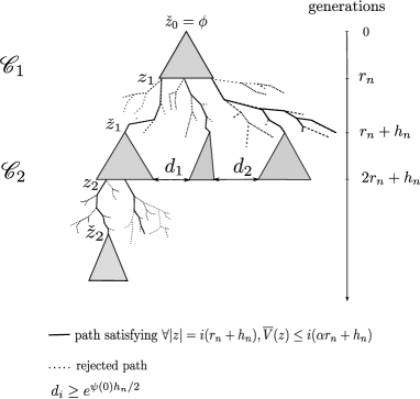
Figure 3: Clusters at regular cuts

We now prove the existence of such clusters, this implies new constraints on ${\bf k}$, ${\bf r}$ and ${\bf s}$ in addition to (4.1).

First, ellipticity conditions imply that for any site $z>y$, ${V}(z)-V(y)\leq\alpha(|z|-|y|)$ a.s. Thus, for all $a\in\mathbb{N}$ and $b>0$, $\{\exists\check{z}>z,|\check{z}|=|z|+a,\tilde{V}(z,\check{z})\leq b\}$ is a.s. contained in $\{{V}(z)-V(y)\leq\alpha(|z|-|y|),\exists\check{z}>z,|\check{z}|=|z|+a,\tilde{V}(y,\check{z})\leq\alpha(|z|-|y|)+b\}$ ($\tilde{V}$ is defined in the proof of (2.6)).
Then, with our slight abuse of notation, a.s. $\mathscr{B}:=\{$the clusters $\mathcal{C}_{.}(.)$ exist$\}$ contains

$$\bigcap_{i=1}^{k_{n}}\left\{\bigcap_{z_{i}\in\mathcal{C}_{ir_{n}+(i-1)h_{n}}(\check{z}_{i-1})}\left\{\exists\check{z}_{i}>z_{i},|\check{z}_{i}|=i(r_{n}+h_{n}),\tilde{V}(z_{i},\check{z}_{i})\leq s_{n}\right\}\right\}.$$

The independence of the increments of $V$ and the ellipticity assumptions on the number of descendants ($|\mathcal{C}_{.}(.)|\leq N_{0}^{r_{n}}$) imply

$$P(\mathscr{B}) \geq\left[P(\exists|{z}|=h_{n},\overline{V}({z})\leq s_{n})\right]^{N_{0}^{k_{n}r_{n}}}=\left[P\left(\min_{|{z}|=h_{n}}\overline{V}({z})\leq s_{n}\right)\right]^{N_{0}^{k_{n}r_{n}}}.$$

Assuming ${\bf s}\geq(1+\zeta-{\bf k})/3$, Lemma 2.3 yields $P(\mathscr{B})\geq(1-\lambda_{h_{n}})^{N_{0}^{k_{n}r_{n}}}\sim\exp\left(-N_{0}^{k_{n}r_{n}}\lambda_{h_{n}}\right)$. To choose $\bf k$, $\bf r$ and $\bf s$, we have to take into account the last constraint in (4.1), $\bf s\leq 1-\bf k$ and that if $q_{0}+q_{1}\neq 0$, $\bf k+\bf r<s$. We distinguish two cases

• if $0<\zeta\leq 1$, let $0<\delta<\zeta/2$, take ${\bf s}=(1+\zeta)/2-\delta$, ${\bf k}=\delta/2$, and ${\bf r}={(1-\zeta)}/{2}+\nicefrac{{\delta}}{{2}}$,

• if $1<\zeta<2$, let $0<\delta<(2-\zeta)/3$, take ${\bf s}=(1+\zeta)/3$, ${\bf k}=\delta$ and ${\bf r}=(1+\zeta-4\delta)/3$.

Thus in both cases

$$P(\mathscr{B}) \geq 1-C_{+}e^{-c_{1}s_{n}}N_{0}^{k_{n}r_{n}}\underset{n\rightarrow+\infty}{\longrightarrow}1.$$ (4.3)

When $q_{0}+q_{1}=0$, the above choices give an even better rate of convergence for $P(\mathscr{B})$.
We now move back to (4.2), (4.3) together with the fact that $\Phi(n)\leq\log n+o(\log n)$ implies

$$\lim_{n\rightarrow+\infty}\mathbb{P}\left(\bigcap_{i=1}^{k_{n}}\bigcap_{\mathcal{D}\in\mathscr{C}_{i}}\bigcap_{z\in\mathcal{D}}\left\{{\mathcal{L}(z,T_{\phi}^{n^{1-\varepsilon}})\geq 1}\right\},\mathscr{B}\right)=1.$$

According to (3.14), as $\mathbb{P}(n\geq T_{\phi}^{n^{1-\varepsilon}})$ tends to one we finally obtain

$$\lim_{n\rightarrow+\infty}\mathbb{P}\left(\bigcap_{i=1}^{k_{n}}\bigcap_{\mathcal{D}\in\mathscr{C}_{i}}\bigcap_{z\in\mathcal{D}}\left\{{\mathcal{L}(z,n)\geq 1}\right\},\mathscr{B}\right)=1.$$

So we can find set of clusters at regular cuts on the tree which are fully visited. To finish the proof of (1.11) we first show the existence of a lower bound for the number of visited clusters. Using successively that conditionally on $\mathscr{B},\,|\mathscr{C}_{i}|$ is equal in law to $Z_{(i-1)r_{n}}$, Theorem A.2 and (4.3)

$$P\left(\exists i\in\llbracket 2,k_{n}\rrbracket,|\mathscr{C}_{i}|\leq e^{\psi(0)(i-1)r_{n}/2}\right) \leq P\left(\exists i\in\llbracket 2,k_{n}\rrbracket,|\mathscr{C}_{i}|\leq e^{\psi(0)(i-1)r_{n}/2},\mathscr{B}\right)+P(\overline{\mathscr{B}})$$

$$\leq\sum_{i=2}^{k_{n}}P\left(Z_{(i-1)r_{n}}\leq e^{\psi(0)(i-1)r_{n}/2}\right)+P(\overline{\mathscr{B}})$$

$$\leq e^{-\psi(0)\nu r_{n}/4}+C_{+}e^{-c_{1}s_{n}}N_{0}^{k_{n}r_{n}}.$$

Note that for the first term we have used the left tail of $Z_{.}$ with $q_{0}+q_{1}>0$ as the other case provide an even better rate of convergence. Finally we prove that the previously defined visited clusters are very spaced out. Recalling the definition of ${\bf D}$ before Theorem 1.2,

$$P\left(\exists i\in\llbracket 2,k_{n}\rrbracket,{\bf{D}}(\mathscr{C}_{i})\leq e^{\psi(0)h_{n}/2}\right) \leq P(\overline{\mathscr{B}})+\sum_{i=2}^{k_{n}}P\left({\bf{D}}(\mathscr{C}_{i})\leq e^{\psi(0)h_{n}/2},\mathscr{B}\right)$$

$$\leq P(\overline{\mathscr{B}}) +\sum_{i=2}^{k_{n}}P\left(\bigcup_{\mathcal{D}\in\mathscr{C}_{i-1}}\bigcup_{z\in\mathcal{D}}\{|\mathcal{C}_{i(r_{n}+h_{n})}(z)|\leq e^{\psi(0)h_{n}/2}\}\cap\mathscr{B}\right).$$

As conditionally on $\mathscr{B},\,|\mathcal{C}_{i(r_{n}+h_{n})}(z)|$ and $Z_{h_{n}}$ are equal in law, on $\mathscr{D}_{i}:=\{|\mathscr{C}_{i}|\leq e^{2\psi(0)(i-1)r_{n}}\},$ $|\mathcal{D}|\,|\mathscr{C}_{i}|\leq N_{0}^{r_{n}}e^{2\psi(0)(i-1)r_{n}}$ so Theorem A.2 yields

$$P\left({\bf{D}}(\mathscr{C}_{i})\leq e^{\psi(0)h_{n}/2},\mathscr{B}\right) \leq P\left(\bigcup_{\mathcal{D}\in\mathscr{C}_{i-1}}\bigcup_{z\in\mathcal{D}}\{|\mathcal{C}_{i(r_{n}+h_{n})}(z)|\leq e^{\psi(0)h_{n}/2}\}\cap\mathscr{B}\cap\mathscr{D}_{i}\right)+P(\overline{\mathscr{D}}_{i})$$

$$\leq e^{r_{n}\log N_{0}+2\psi(0)(i-1)r_{n}}P(Z_{h_{n}}\leq e^{\psi(0)h_{n}/2})+e^{-\psi(0)(i-1)r_{n}}$$

$$\leq e^{r_{n}\log N_{0}+2\psi(0)(i-1)r_{n}-\nu\psi(0)h_{n}/2}+e^{-\psi(0)(i-1)r_{n}}.$$

Consequently

$$P\left(\exists i\in\llbracket 2,k_{n}\rrbracket,{\bf{D}}(\mathscr{C}_{i})\leq e^{\psi(0)h_{n}/2}\right)\leq e^{3\psi(0)k_{n}r_{n}-\nu\psi(0)h_{n}/2}+2e^{-\psi(0)r_{n}}+C_{+}e^{-c_{1}s_{n}}N_{0}^{k_{n}r_{n}},$$

moreover as $h_{n}\sim(\log n)^{1+\zeta-\bf{k}}$, ${\bf k}+{\bf r}<{\bf s}<1$ and ${\bf k}<\zeta$ we obtain the result.

4.2 Proof of (1.10)

Let $m=\varepsilon\ell^{1/3}$, $\delta>0$, define $\mathcal{B}$ the set of points $z^{\prime}$ such that for all $|z|=m$, $z^{\prime}:={\bf inf}\{u>z,|u|=\ell,\overline{V}(u)\leq\Phi(n)(1-\delta)\}$. Corollary C.1 gives

$$\mathbb{P}^{\mathcal{E}}\left(\bigcup_{z^{\prime}\in\mathcal{B}}\left\{\mathcal{L}(z^{\prime},T_{\phi}^{n^{1-\varepsilon}})=0\right\}\right)\leq|\mathcal{B}|e^{-c_{-}n^{1-\varepsilon}e^{-\Phi(n)(1-{\delta})}/\ell}\leq Z_{m}e^{-c_{-}n^{1-\varepsilon}e^{-\Phi(n)(1-{\delta})}/\ell}.$$

As $\Phi(n)\leq\log n+o(\log n)$ and $E[Z_{m}]=e^{\psi(0)m}$, taking $\delta=2\varepsilon$

$$\mathbb{P}\left(\bigcup_{z^{\prime}\in\mathcal{B}}\left\{\mathcal{L}(z^{\prime},T_{\phi}^{n^{1-\varepsilon}})=0\right\}\right)\leq e^{-c_{-}n^{\varepsilon/2}}.$$ (4.4)

We now prove that $\lim_{n\rightarrow+\infty}P(|\mathcal{B}|=Z_{m})=1$. From [14] (see also [3] Lemma 2.1), $\lim_{n\rightarrow+\infty}P(\max_{|z|=m}\overline{V}(z)\leq 2\tilde{\gamma}m)=1$, so as for $n$ large enough $\ell^{1/3}/\Phi(n)\leq\delta$ with the same arguments used in the proof of Lemma 2.3

$$P(|\mathcal{B}|<Z_{m}) \leq P\left(\bigcup_{|z|=m}\left\{\forall z^{\prime}>z,|z^{\prime}|=\ell,\overline{V}(z^{\prime})>(1-\delta)\Phi(n)\right\}\right)$$

$$\leq 1-\left(1-P\left(\min_{|z|=\ell-m}\overline{V}(z)>(1-2\delta)\Phi(n)\right)\right)^{e^{2\psi(0)m}}+e^{-\psi(0)m}$$

$$\leq 2P\left(\min_{|z|=\ell-m}\overline{V}(z)>(1-4\varepsilon)\Phi(n)\right)e^{2\psi(0)m}+e^{-\psi(0)m}.$$

To finish we put ourself in the case $q_{0}+q_{1}>0$ (the other case is treated similarly), using Lemma 2.3

$$P\left(\min_{|z|=\ell-m}\overline{V}(z)>(1-4\varepsilon)\Phi(n)\right)\leq e^{-c_{1}\ell^{1/3}}.$$

We can now choose $\varepsilon$ small enough and obtain, $P(|\mathcal{B}|=Z_{m})\geq 1-e^{-c_{1}\ell^{1/3}/2}$. Moving back to (4.4) $\mathbb{P}(\forall z\in\mathcal{B},\mathcal{L}(z,T_{\phi}^{n^{1-\varepsilon}})\geq 1,|\mathcal{B}|=Z_{m})\geq 1-o(1)$. Finally to obtain (1.10) we apply (3.14).

Appendix A Basic facts for branching processes and Galton-Watson trees

A.1 Biggins-Kypriaou identities and properties of $\boldsymbol{\psi}$

For any $n\geq 1$ and any mesurable function $F:\mathbb{R}^{n}\rightarrow[0,+\infty)$, Biggins-Kyprianou identity is given by

$$E\left[\sum_{|x|=n}e^{-V(x)}F(V(x_{i}),1\leq i\leq n)\right]=E[F(S_{i},1\leq i\leq n)]$$ (A.1)

where $(S_{i}-S_{i-1})_{i\geq 1}$ are i.i.d. random variables, and the law of $S_{1}$ is determined by

$$E[f(S_{1})]=E\left[\sum_{|x|=1}e^{-V(x)}f(V(x))\right],$$ (A.2)

for any measurable function $f:\mathbb{R}\rightarrow[0,+\infty)$. A proof can be found in [5], see also [18]. We have the following identities

$$\psi(t)=\log E[e^{(1-t)S_{1}}],\psi^{\prime}(t)=-\frac{E[S_{1}e^{(1-t)S_{1}}]}{E[e^{(1-t)S_{1}}]}.$$

In particular, $E[N]=e^{\psi(0)}=E[e^{S_{1}}]$ and the hypothesis $\psi^{\prime}(1)=0$ equates to $E[S_{1}]=0$.

Remark A.1

Let $\alpha:=|\log\varepsilon_{0}|$, we have $\mathbb{P}(|S_{1}|\leq\alpha)=1$. Indeed taking $f(x)=\mathds{1}_{|x|\leq\alpha}$ and using Biggins-Kiprianou, $\mathbb{P}(|S_{1}|\leq\alpha)=E[f(S_{1})]=e^{\psi(1)}=1$.

A.2 Left tail of $\boldsymbol{Z_{n}}$

Recall that the positive martingale $(W_{n})_{n\geq 0}:=(\nicefrac{{Z_{n}}}{{e^{\psi(0)n}}})_{n\geq 0}$ converges a.s. to a non degenerate limit $W$ (see for instance [18]). Moreover $W$ has a positive continuous density function denoted $w$. Bingham [6] shows that for the Schröder case ($q_{0}+q_{1}>0$), there exists $0<\nu<1$ such that for small $x$, $w(x)\sim x^{\nu-1}$ and for the Böttcher case ($q_{0}+q_{1}=0$) there exists $\beta\in(0,1)$ such that when $x\rightarrow 0$, $\log w(x)\sim-{x^{-\frac{\beta}{1-\beta}}}$. The results of [4] and then [10] (Theorems 4 and 5) and [11] (Theorem 7) lead to

Theorem A.2

Let $0<\kappa<1$ then $P(Z_{n}\leq e^{\kappa\psi(0)n})\sim e^{-\nu\psi(0)(1-\kappa)n}$ in the Schröder case, and $\log P(Z_{n}\leq e^{\kappa\psi(0)n})\sim\log w\left({e^{\psi(0)(\kappa-1)n}}\right)$ in the Böttcher case.

Appendix B Results for sums of i.i.d. random variables

In this section we recall basic facts for sum of i.i.d. random variables applied to $(S_{n})_{n\geq 0}$ of Section A. Recall that for all $x\in\mathbb{R}$, $\tau_{x}^{+}=\inf\{n\geq 1,S_{n}\geq x\}$ and $\tau_{x}^{-}=\inf\{n\geq 1,S_{n}\leq x\}$. The following results are standard and can be found in [1] and [19].

Lemma B.1

For all $x\in[0,y]$ and $m$ large enough

$$P_{x}(\tau^{+}_{y}<\tau^{-}_{0})\asymp\frac{x+1}{y+1},\ E[\tau^{+}_{y}\wedge\tau^{-}_{0}]\asymp y\mbox{ and }P_{x}(\tau^{-}_{0}>m)\asymp\frac{x+1}{\sqrt{m}}.$$

Recalling that for all $n\geq 1$, $Y^{-}(n)=\sum_{i=1}^{n}e^{-S_{i}}$, we have

Lemma B.2

There exists a constant $C_{+}>1$ such that for all $a\geq 0$ and $M>0$

$$P\left(Y^{-}(\tau_{a}^{+})>M,\ \tau^{+}_{a}<\tau^{-}_{0}\right)\leq\nicefrac{{C_{+}}}{{M}}.$$

Proof.
According to [2] p.19, there exists $C_{+}>1$ such that for all $0\leq a\leq L\leq 1$,

$$\mathbb{E}\left[Y^{-}({\tau^{-}_{0}\wedge\tau^{+}_{a}})\right]\leq C_{+}\nicefrac{{a+1}}{{a}}.$$

As $P\left(Y^{-}(\tau_{a}^{+})>M,\ \tau^{+}_{a}<\tau^{-}_{0}\right)\leq P\left(Y^{-}({\tau^{-}_{0}\wedge\tau^{+}_{a}})>M\right)$, we conclude using the Markov inequality. $\blacksquare$

Lemma B.3

For any $m\geq 1$,

$$E[e^{S_{m}}\mathds{1}_{\tau_{0}^{-}>m}]\asymp{(m+1)^{-3/2}}.$$ (B.1)

Proof.
The upper bound can be found in [13] p.44, the lower bound can be obtained as follows: $E[e^{S_{m}}\mathds{1}_{\tau_{0}^{-}>m}]\leq\sum_{k=0}^{\alpha m}e^{-k}P(S_{m}\in[-k,-k+1],\bar{S}_{m}<0)=\sum_{k=0}^{\alpha m}ke^{-k}m^{-3/2}\asymp{(m+1)^{-3/2}}$. $\blacksquare$

Recalling that for all $n\geq 1$, $Y^{-}(n)=\sum_{i=1}^{n}e^{-S_{i}}$, we have

Lemma B.4

There exists a constant $C_{+}>1$ such that for all $a\geq 0$ and $M>0$

$$P\left(Y^{-}(\tau_{a}^{+})>M,\ \tau^{+}_{a}<\tau^{-}_{0}\right)\leq\nicefrac{{C_{+}}}{{M}}.$$

The following Lemma may be found in the literature, however as we can prove it easily for our case we present a short proof.

Lemma B.5

Let $m>1$, assume that $b=b(m)\geq\sigma^{2}\sqrt{m}\log m$, with $\lim_{m\rightarrow+\infty}b/m=0$, and $a=a(m)>0$ is such that $\lim_{m\rightarrow+\infty}a/\sqrt{m}=0$, then for all $m$ large enough

$$P_{a}\left({S}_{m}>b,\underline{S}_{m}>0\right)\leq C_{+}\frac{a}{b}e^{b\cdot g(b/m)},$$ (B.2)

with $g(x)=f(x)-1=-\frac{x}{2\sigma^{2}}+x^{2}\lambda(x).$ For all $\varepsilon>0$ and $r>\varepsilon m$.

$$P_{a}\left({S}_{m}\geq r,\underline{S}_{m}>0\right)\leq C_{+}\frac{a}{\sqrt{m}}e^{-sr+m\psi(1-s)}.$$ (B.3)

Proof.
For (B.2), let $\omega$ a positive function of $b$ and $m$, such that $\omega\leq 2\sqrt{m}/b$ and that we choose later, write $P_{a}\left({S}_{m}>b,\underline{S}_{m}>0\right)$ as

$$P_{a}\left({S}_{m}>b,\underline{S}_{m}>0,\tau^{+}_{\sqrt{m}}\leq\omega m\right)+P_{a}\left({S}_{m}>b,\underline{S}_{m}>0,\tau^{+}_{\sqrt{m}}>\omega m\right)=:P_{3}+P_{4}.$$

Strong Markov property and homogeneity give:

$$P_{a}\left({S}_{m}>b,\underline{S}_{m}>0,\tau^{+}_{\sqrt{m}}=j\right) \leq P_{a}\left(\tau^{-}_{0}>\tau^{+}_{\sqrt{m}}=j\right)\sup_{0\leq x\leq\alpha}P_{\sqrt{m}+x}\left({S}_{m-j}>b,\underline{S}_{m-j}>0\right)$$

$$\leq P_{a}\left(\tau^{-}_{0}>\tau^{+}_{\sqrt{m}}=j\right)P\left({S}_{m-j}>b-\sqrt{m}-\alpha\right)$$

implying with Lemma B.1:

$$P_{4} \leq\sum_{j=\omega m+1}^{m}P_{a}\left(\tau^{-}_{0}>\tau^{+}_{\sqrt{m}}=j\right)P\left({S}_{m-j}>b-\sqrt{m}-\alpha\right)$$

$$\leq P_{a}\left(\tau^{-}_{0}>\tau^{+}_{\sqrt{m}}\right)\sup_{\omega m\leq j\leq m}P\left({S}_{m-j}>b-\sqrt{m}-\alpha\right)$$

$$\leq C_{+}\frac{a}{\sqrt{m}}\sup_{\omega m\leq j\leq m}P\left({S}_{m-j}>b-\sqrt{m}-\alpha\right),$$

A classical result of moderate deviations (see for instance [17], Chapter VIII, Theorem 1) implies

$$P\left({S}_{m(1-\omega)}>b-\sqrt{m}-\alpha\right) \leq\frac{C_{+}\sqrt{m(1-\omega)}}{(b-\sqrt{m}-\alpha)}e^{(b-\sqrt{m}-\alpha)g((b-\sqrt{m}-\alpha)/(m(1-\omega)))}$$

$$\sim\frac{C_{+}\sqrt{m}}{b}e^{(b-\sqrt{m})g((b-\sqrt{m})/(m(1-\omega)))}$$

We now choose $\omega$ in such a way that $(b-\sqrt{m})g((b-\sqrt{m})/(m(1-\omega)))-bg(b/m)=O(1)$, $\omega$ is actually a sum which first two terms are $\omega=2m^{1/2}/b-\lambda(b/m)/\sqrt{m}+...$. So for any $n$ large enough

$$P\left({S}_{m(1-\omega)}>b-\sqrt{m}-\alpha\right) \leq\frac{C_{+}\sqrt{m}}{b}e^{b\cdot g(b/m)}.$$

With similar computations this upper bound is still true for $P\left({S}_{m-j}>b-\sqrt{m}-\alpha\right)$ for $m(1-\varepsilon)\leq j\leq m$, so $P_{4}\leq C_{+}\frac{a}{{b}}e^{bg(b/m)}$. In the same way

$$P_{3} \leq\sum_{j=\sqrt{m}/\alpha}^{\omega m}P_{a}\left(\tau^{-}_{0}>\tau^{+}_{\sqrt{m}}=j\right)\sup_{0\leq x\leq\alpha}P_{\sqrt{m}+x}\left({S}_{m-j}>b,\underline{S}_{m-j}>0\right)$$

$$\leq\sum_{j=\sqrt{m}/\alpha}^{\omega m}P\left(S_{j}\geq{\sqrt{m}}-a\right)P\left({S}_{m-j}>b-\sqrt{m}-\alpha\right),$$

Using again [17],

$$P_{3} \leq C_{+}\sum_{j=\sqrt{m}/\alpha}^{\omega m}\frac{j^{1/2}}{\sqrt{m}-a}e^{-m/(2\sigma^{2}j)}\frac{(m-j)^{1/2}}{b-\sqrt{m}-\alpha}e^{(b-\sqrt{m}-\alpha)g((b-\sqrt{m}-\alpha)/(m-j))}$$

$$\leq C_{+}\frac{(\omega m)^{1/2}}{b}e^{-b/(2\sigma^{2}m^{1/2})}e^{b\cdot g(b/m)}=o\left(\frac{e^{b\cdot g(b/m)}.}{b}\right).$$

which finish the proof. (B.3) can be proved in a similar way with classical large deviation estimates. $\blacksquare$

The following Lemma states the local behavior of sums of i.i.d. random variables, recall that $S_{1}$ is non-lattice.

Lemma B.6

Let $\varepsilon>0$ small and $A>0$ large. For all $m$ large enough, for all $1\leq r\leq A\sqrt{m}$

$$P\left({S}_{m}\in(r,r+1],\underline{S}_{m}>0\right)=\frac{r}{m^{3/2}}e^{-r^{2}/(2\sigma^{2}m)}+o(m^{-3/2}).$$ (B.4)

For all $A\sqrt{m}\leq r\leq\varepsilon m$

$$P\left({S}_{m}\in(r,r+1],\underline{S}_{m}>0\right)\asymp\frac{1}{m}e^{rg(r/m)}.$$ (B.5)

see Lemma B.5 for the definition of $g$.

Proof.
(B.4) is F. Caravenna [7] result and (B.5) can be obtained with [17] Chapter VIII, Theorem 2 and 10 and similar arguments than in the proof of Lemma B.5. $\blacksquare$

Appendix C Probability of hitting time

Lemma C.1

For $x^{\prime}\in\llbracket\phi,x\rrbracket$:

$$\mathbb{P}_{x^{\prime}_{x}}^{\mathcal{E}}(T_{x}<T_{x^{\prime}}) = \frac{e^{V(x^{\prime}_{x})}}{\sum_{z\in\rrbracket x^{\prime},x\rrbracket}e^{V(z)}},$$ (C.1)

$$\mathbb{P}_{\overset{\leftarrow}{x}}^{\mathcal{E}}(T_{x^{\prime}}<T_{x}) = \frac{e^{V(x)}}{\sum_{z\in\rrbracket x^{\prime},x\rrbracket}e^{V(z)}}.$$ (C.2)

where $x^{\prime}_{x}$ is the only children of $x^{\prime}$ in $\llbracket x^{\prime},x\rrbracket$.

The result is classical (see for instance [3]) and a useful direct consequence of this latter is the following

Corollary C.1

Let $\mathcal{A}\subset\{z\in\mathbb{T},|z|=\ell\}$ and $\kappa>0$, there exists a positive constant $c_{7}$ such that

$$\mathbb{P}^{\mathcal{E}}_{\phi}(T_{\phi}^{n^{\kappa}}<T_{z}) \leq\exp\left(-c_{7}n^{\kappa}e^{{\overline{V}(z)}}/{\ell}\right),\,\forall z\in\mathcal{A},$$ (C.3)

$$\mathbb{P}^{\mathcal{E}}\left(\bigcup_{z\in\mathcal{A}}\{\mathcal{L}(z,T_{\phi}^{n^{\kappa}})=0\}\right) \leq|\mathcal{A}|\exp\left(-c_{7}n^{\kappa}e^{-{\max_{z\in\mathcal{A}}\overline{V}(z)}}/{\ell}\right)$$ (C.4)

Proof.
Obviously (C.4) is a consequence of (C.3). Thanks to formula (C.1), for $z\in\mathcal{A}$, $\mathbb{P}^{\mathcal{E}}_{\phi}\left(T_{z}<T_{\phi}\right)$ $\geq C_{-}e^{-\overline{V}(z)}/\ell$. Then using the strong Markov property and the recurrence of $X$, for $n$ large enough $\mathbb{P}^{\mathcal{E}}_{\phi}\left(T_{\phi}^{n^{\kappa}}<T_{z}\right)=(1-\mathbb{P}^{\mathcal{E}}_{\phi}\left(T_{z}<T_{\phi}\right))^{n^{\kappa}}\leq\exp\left(e^{-c_{7}n^{\kappa}{\overline{V}(z)}}/{\ell}\right).$ $\blacksquare$

References

- [1] E. Aidékon. Tail asymptotics for the total progeny of the critical killed branching random walk. Elec. Comm. in Probab., 15:522–533, 2010.
- [2] E. Aidékon, Y. Hu, and O. Zindy. The precise tail behavior of the total progeny of a killed branching random walk. To appear in Annals of Probability.
- [3] P. Andreoletti and P. Debs. The number of generations entirely visited for recurrent random walks on random environment. J. Theoret. Probab., To be published.
- [4] K.B. Athreya and P.E. Ney. Branching processes. Springer-Verlag, 1972.
- [5] J.D. Biggins and A.E. Kyprianou. Senata-heyde norming in the branching random walk. Ann. Probab., 25: 337–360, 1997.
- [6] N. H. Bingham. On the limit of a supercritical branching process. Journal of Applied Probability, 25: 245–228, 1988.
- [7] F. Caravenna. A local limit theorem for random walks conditioned to stay positive. Probab. Theory Related Fields, 133: 508–530, 2005.
- [8] G. Faraud. A central limit theorem for random walk in a random environment on marked galton-watson trees. Electronic Journal of Probability, 16(6):174–215, 2011.
- [9] G. Faraud, Y. Hu, and Z. Shi. Almost sure convergence for stochastically biased random walks on trees. to appear in Probab. Theory Relat. Fields, 2011.
- [10] K. Fleischmann and V. Wachtel. Lower deviation probabilities for supercritical galtonÐwatson processes. Ann. I.H.P., 43: 233–255, 2007.
- [11] K. Fleischmann and V. Wachtel. On the left tail asymptotics for the limit law of a supercritical galton-watson processes in the bötcher case. Ann. I.H.P., 45: 201–225, 2009.
- [12] Y. Hu and Z. Shi. Slow movement of recurrent random walk in random environment on a regular tree. Ann. Probab., 35:1978–1997, 2007.
- [13] Y. Hu and Z. Shi. Minimal position and critical martingale convergence in branching random walks, and directed polymers on disordered trees. Ann. Probab., 37:742–789, 2009.
- [14] C. McDiarmid. Minimal position in a branching random walk. Ann. Appl. Proba., 5(1): 128–139, 1995.
- [15] M.V. Menshikov and D. Petritis. On random walks in random environment on trees and their relationship with multiplicative chaos. Math. Comput. Sci., 415-422, 2002.
- [16] J. Neveu. Arbres et processus de galton-watson. Ann. de l’IHP, 22(2), 1986.
- [17] V.V. Petrov. Sums of Independent Random Variables. Springer-Verlag, 1975.
- [18] Z. Shi. Random walks and trees. ESAIM: Proceedings, 31: 1–39, (2011).
- [19] F. Spitzer. Principle of Random Walks. Van Nostrand, Princeton N.J., 1964.