Background fitting of Fermi GBM observations

Abstract

The Fermi Gamma-ray Burst Monitor (GBM) detects gamma-rays in the energy range 8 keV - 40 MeV. We developed a new background fitting process of these data, based on the motion of the satellite. Here we summarize this method, called Direction Dependent Background Fitting (DDBF), regarding the GBM triggered catalog. We also give some preliminary results and compare the duration parameters with the 2-years Fermi Burst Catalog.

I Introduction

Fermi has specific proper motion when surveying the sky. It is designed to catch gamma-ray bursts in an effective way. However, bursts can have a varying background, especially in the case of the Autonomous Repoint Request (ARR). Modeling this with a polynomial function of time is not efficient in many cases. Here we present the effect of these special moving feature, and we define direction dependent underlying variables. We use them to fit a general multidimensional linear function for the background.

Note that here we give a short summary of the method and some preliminary results. The detailed description of the Direction Dependent Background Fitting (DDBF) algorithm and the final results will be published soon (Szécsi et al., 2013).

II Fermi lightcurves with varying background

Fermi’s slewing algorithm is quite complex. It is designed to optimize the observation of the Gamma-Ray Sky. In Sky Survey Mode, the satellite rocks around the zenith within $\pm 50^{\circ}$, and the pointing alternates between the northern and southern hemispheres each orbit (Meegan et al., 2009; Fitzpatrick, 2011). In Autonomous Repoint Request (ARR) mode, it turns toward the burst and stays there for hours. 12 NaI detectors are placed such a way that the entire hemisphere is observable with them at the same time.

The GBM data, which we use in our analysis (called CTIME), are available at 8 energy channels, with $0.064$-second for triggered and $0.264$-second resolution for non-triggered mode. The position data is available in $30$-second resolution. This data were evenly proportioned to $0.256$-second and $0.064$-second bins using linear interpolation, in order to correspond to the CTIME data (Meegan et al., 2009).

Using GBM data, 1-second bins and summarizing the counts in the channels between 11.50–982.23 keV, one can plot a GBM lightcurve as shown in Fig. 1.

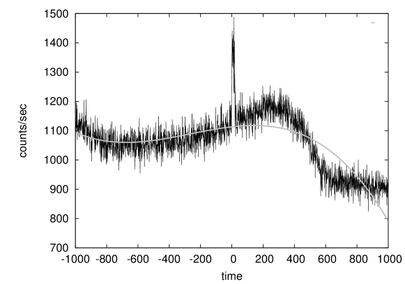
Figure 1: Lightcurve of the Fermi burst 091030613 measured by the 3rd GBM-detector, without any background filtering, with 1-second bins. The grey line is a fitted polynomial function of time of order 3.

III Direction Dependent Background Fitting (DDBF)

Analyzing ancillary spacecraft and other directional data we have found the following $(\mathbf{x}_{i})$ variables, which seem to contribute to the variation of the background: celestial distance between burst and detector orientation, celestial distance between Sun and detector orientation, rate of the Earth-uncovered sky and time (Szécsi et al., 2013).

We use the method of General Least Square for multidimensional fitting of the $\mathbf{y_{i}}$ counts to the corresponding $(\mathbf{x})$ explanatory variables. The maximum likelihood estimate of the model parameters $a_{k}$ is obtained by minimizing the quantity of

$$\chi^{2}=\Sigma_{i=1}^{N}\left(\frac{y_{i}-\Sigma_{k=1}^{M}a_{k}X_{k}(\mathbf{x}_{i})}{\sigma_{i}}\right)^{2}$$ (1)

The matrix of $A$ and vector $\mathbf{b}$ are:

$$A_{ij}=\frac{X_{j}(\mathbf{x}_{i})}{\sigma_{i}},\hskip 20.0ptb_{i}=\frac{y_{i}}{\sigma_{i}}.$$ (2)

Minimizing $\chi^{2}$ leads us to the following equation:

$$\mathbf{a}=(\mathbf{A}^{T}\mathbf{A})^{-1}\mathbf{A}^{T}\mathbf{b},$$ (3)

, where $\mathbf{A}^{T}$ means the transpose of $\mathbf{A}$, and the expression $(\mathbf{A}^{T}\mathbf{A})^{-1}\mathbf{A}^{T}$ are called generalized inverse or pseudoinverse of $\mathbf{A}$. For calculating the pseudoinverse of the design matrix $\mathbf{A}$ we used Singular Value Decomposition (SVD): $\mathbf{A}=\mathbf{US}{V}^{T}$. Using $\mathbf{U}$ and $\mathbf{V}$, the pseudoinverse of $\mathbf{A}$ can be obtained as

$$pinv(\mathbf{A})=(\mathbf{A}^{T}\mathbf{A})^{-1}\mathbf{A}^{T}=\mathbf{VS}^{-1}\mathbf{U}^{T}.$$ (4)

Since we want to have a method for all the Fermi bursts, we define our model to be quite comprehensive. Let us have $y(\mathbf{x}_{i})$ as the function of $\mathbf{x}_{i}=(x^{(1)}_{i},x^{(2)}_{i},x^{(3)}_{i},x^{(4)}_{i})$ of order 3, so the basis functions $X_{k}(\mathbf{x}_{i})$ (and columns of the design matrix) consist of every possible products of the components $x^{(l)}_{i}$ up to order 3. That means that we have $M=k_{max}=35$ basis functions and $a_{1}$, $a_{2}$…$a_{35}$ free parameters. It is sure that we do not need so many free parameters to describe a simple background. Computing the pseudoinverse we need the reciprocal of the singular values in the diagonals of $\mathbf{S}^{-1}$, but if we compute the pseudoinverse of $\mathbf{A}$, the reciprocals of the tiny and not important singular values will be unreasonably huge and enhance the numerical roundoff errors as well. This problem can be solved defining a limit value, below which reciprocals of singular values are set to zero (Szécsi et al., 2013).

One cornerstone of the fitting algorithm described above is the definition of the boundaries which divide the interval of the burst and the intervals of the background. In this work, we follow the common method of using user-selected time intervals (Paciesas et al., 2012). But unlike Paciesas et al. (2012), using the position data allows us to fit the total CTIME file instead of selecting two small intervals around the burst (Szécsi et al., 2013).

IV Model selection

The Akaike Information Criterion (AIC) is a commonly used method of choosing the right model to the data (Akaike, 1974). Assume that we have $M$ models so that the $k$th model has $k$ free parameters ($k=1...M$). When the deviations of the observed values from the model are normally and independently distributed, every model has a value AIC_k so that

$$\mathrm{AIC}_{k}=N\cdot\log{\frac{RSS_{k}}{N}}+2\cdot k$$ (5)

, where $RSS_{k}$ is the Residual Sum of Squares from the estimated model ($RSS=\Sigma_{i=1}^{N}\left(y_{i}-y(\mathbf{x}_{i},k)\right)^{2}$), $N$ is the sample size and $k$ is the number of free parameters to be estimated. Given any two estimated models, the model with the lower value of AIC_k is the one to be preferred. Given many, the one with lowest AIC_k will be the best choice: it has as many free parameters as it has to have, but not more.

We loop over the pseudoinverse operation and choose $S_{kk}$ as the limit of singular values in the $k$th step, and compute the corresponding AIC_k. The number of singular values which minimalize the AIC_k as a function of $k$ will be the best choice when calculating the pseudoinverse (Szécsi et al., 2013).

As an example we analyze the lightcurve of GRB 090113778. GRB 090113 is a long burst with T${}_{90}^{cat}$=17.408$\pm$3.238 s in the GBM Catalogue, here we show Detector 0 data:

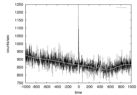
Figure 2: Up: Lightcurve of the Fermi GRB 090113778 measured by the triggered GBM-detector ’8’, and the fitted background with a grey line. Burst interval (secs): [-20:40]. Down: Underlying variables (absolute values).

Figure 3: Down left: Akaike Information Criterion. A model with 12 singular values was selected. Down right: Cumulated lightcurve of GRB 090113778.

Fig. 2 has some extra counts around 400 and 600 seconds. Both of them can be explained with the variation of the underlying variables, that is, the motion of the satellite. These are not GRB signals!

V Error analysis

The DDBF method is too complicated to give a simple expression for the error of $T_{90}$ using general rules of error propagation. We therefore repeated the process for 1000 MC simulated data.

V.1 GRB 090113778

Distribution of the Poisson-modified $T_{90}$ and $T_{50}$ values are shown in Fig. 4 for GRB090113778.

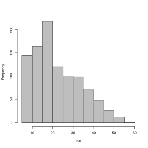
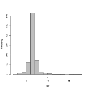
Figure 4: Distibution of the $T_{90}$ (up) and $T_{50}$ (down) values obtained from the MC simulated data for Fermi burst 090113778.

Fig. 4 shows the Monte Carlo simulated distributon of the duration values of GRB 090113778. Based on this, we give confidence intervals corresponding to 68% (1$\sigma$ level). The result is given in Table 1. Table 1. also contains some of our other, preliminary results using DDBF. For more details, see our forthcoming paper Szécsi et al. (2013).

V.2 GRB 091030613

Distribution of the Poisson-modified $T_{90}$ and $T_{50}$ values are shown in Fig. 5 for GRB091030613.

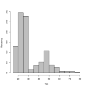
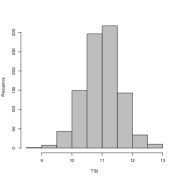
Figure 5: Distibution of the $T_{90}$ (left) and $T_{50}$ (right) values obtained from the MC simulated data for Fermi burst 091030613.

Fig. 4 shows two significant peaks around 22 and 47 seconds. The first peak at 22 seconds corresponds to the measured $T_{90}$ value. However, in some cases of the Poison noise simulation, the measured $T_{90}$ value is systematically longer: that is because this burst has a little pulse around 47 seconds (see Fig. 1.). There is no sign of this second peak in the $T_{50}$ distribution, as it is more robust.

V.3 Preliminary results

In Figures 6-10 show the MC simulated $T_{90}$ and $T_{50}$ values for the GRBs given in Table 1.

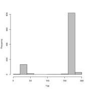
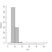
Figure 6: Distibution of the $T_{90}$ (left) and $T_{50}$ (right) values obtained from the MC simulated data for Fermi burst 081009360, GBM detector ’8’.

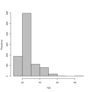
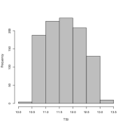
Figure 7: Distibution of the $T_{90}$ (left) and $T_{50}$ (right) values obtained from the MC simulated data for Fermi burst GRB 090102122, GBM detector ’a’.

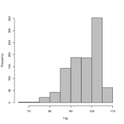
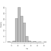
Figure 8: Distibution of the $T_{90}$ (left) and $T_{50}$ (right) values obtained from the MC simulated data for Fermi burst 090618353, GBM detector ’7’.

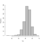
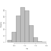
Figure 9: Distibution of the $T_{90}$ (left) and $T_{50}$ (right) values obtained from the MC simulated data for Fermi burst 090828099, GBM detector ’5’.

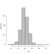
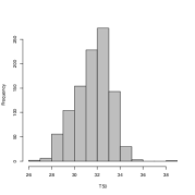
Figure 10: Distibution of the $T_{90}$ (left) and $T_{50}$ (right) values obtained from the MC simulated data for Fermi burst 100130777, GBM detector ’b’.

Burst	$T_{90}(s)$	errors $(s)$		$T_{90}^{catalog}(s)$	$T_{50}(s)$	errors $(s)$		$T_{50}^{catalog}(s)$
081009690	176.228	${+1.357}$	${-9.477}$	176.191	15.852	${+3.006}$	${-2.350}$	25.088
090102122	29.756	${+2.971}$	${-1.198}$	26.624	10.859	${+0.531}$	${-0.556}$	9.728
090113778	19.679	${+10.883}$	${-6.421}$	17.408	6.408	${+0.498}$	${-0.344}$	6.141
090618353	103.338	${+3.842}$	${-6.725}$	112.386	22.827	${+2.201}$	${-1.530}$	23.808
090828099	63.608	${+1.467}$	${-1.652}$	68.417	11.100	${+0.198}$	${-0.194}$	10.752
091030613	22.609	${+13.518}$	${-4.522}$	19.200	10.770	${+0.388}$	${-0.424}$	9.472
100130777	80.031	${+3.755}$	${-3.485}$	86.018	32.340	${+0.931}$	${-1.363}$	34.049

Table 1: Preliminary results and confidence intervals. $T_{90}^{catalog}$ and $T_{50}^{catalog}$ are from the GBM Catalogue (Paciesas et al., 2012).

VI Summary

We summarized the Direction Dependent Background Fitting (DDBF) algorithm which is designed to filter the background of the Fermi lightcurves on a longer timescale (2000 seconds of the CTIME datafile). This technique is based on the motion and orientation of the satellite. The DDBF considers the position of the burst, the Sun and the Earth as well. Based on these position information, we computed three physically meaningful underlying variables, and fitted a 4 dimensional hypersurface on the background. Singular value decomposition and Akaike information criterion was used to reduce the number of free parameters.

One of the main advantage of the DDBF method is that it considers only variables with physical meaning. Furthermore, this method can fit the total 2000 sec CTIME data as opposed to the currently used methods. This features are necessary when analyzing long GRBs and precursors, where motion effects influence the background rate sometimes in a very extreme way. Therefore, not only Sky Survey, but ARR mode GRB’s can be analyzed, and a possible long emission can be detected.

A detailed description of the DDBF method, the first resulst, the comparison with the currently used methods, and analysis of the ARR cases will be published soon (Szécsi et al., 2013).