Object-based High Contrast
Traveltime Tomography

Abstract

We consider a traveltime tomography problem that involves detection of high velocity structures in a homogeneous medium. If we only have limited measurements, this problem becomes an under-determined inverse problem and a common approach would be using prior information to guide the reconstruction process. We restrict the possible velocity into discrete values and model it as a discrete nonlinear inverse problem. However, typical iterative linearized reconstruction algorithms on grid-spacing model usually have very poor reconstruction results in the presence of high contrast boundaries. The reason is that the travel path bends significantly near the boundary, making it very difficult to infer the travel path and velocity value from measured traveltime. To handle this scenario, we propose an object-based approach to model high velocity structures by pre-defined convex objects. Compared to the typical grid-spacing model, which has variables that are proportional to the number of cells, our approach has an advantage that the number of unknown variables in the system is proportional to the number of objects, which greatly decreases the problem dimension. We have developed a fast algorithm to provide an estimate of the appearance probability of high velocity structures in the region of interest. Simulations show that our method can efficiently sample the model parameter space, and provide more robust reconstruction results for the scenario where the number of measurements is limited.

I Introduction

Traveltime tomography aims to reconstruct a velocity model by using the measured first-arrival time between transmitters and receivers. This technique is widely used to characterize the physical properties of elastic media, where the heterogeneous structures lead to different travel velocity. The transmitted signal could be a seismic wave, an acoustic sound wave, and even a fluid pressure wave. For example, traveltime tomography is applied in applications such as seismic geophysical exploration [21], measuring temperature and flow (in air [31] or ocean [17]) and testing aquifer hydraulic properties [32]. However, different from many other tomographic reconstruction problems (e.g., X-Ray or Positron emission computed tomography), where the straight line trajectory assumption is commonly used, in the problems we consider here the travel path may bend severely when it encounters a high contrast velocity abnormality. In many geophysical applications, it is common to have heterogeneous structures that exhibit large differences in velocity between neighboring areas, where the scale of heterogeneous structures is much larger than the effective wavelength. This scenario can be found in different applications: using seismic waves to find permeable fracture zones in ground-water flow characterization [18], monitoring the water/oil saturation in vegetable oil bio-remediation projects [12] and many others. Different from cases where there are only relatively small changes of velocity in the medium, in high contrast medium the travel path not only bends severely but is also dominated by these high velocity structures. Thus the straight ray path approximation is no longer a valid assumption, turning reconstruction of the velocity model into a nonlinear inverse problem. Bent ray reconstruction methods, based on iteratively finding the travel path and updating the velocity model, can be used in this context. However, in many practical situations the available measured traveltime data is very sparse, so that these methods perform poorly due to low ray-coverage and severe path bending near the boundary of high contrast structures. For a comprehensive review on this subject, we refer the reader to the overview by Berryman [4] and to Rawlinson et. al. [23].

This work is motivated by the problem of flow permeability characterization in a fractured reservoir [28]. Waterflooding, as one of the most widely used enhanced oil recovery (EOR) techniques, involves injecting water in a controlled manner in order to offer pressure support that can slowly sweep oil into the production wells [30]. During this process, the permeability of open fractures can be orders of magnitude higher than that of surrounding tight rocks, providing fast pathways for the flow. Thus, traveltime through a fracture is much faster than through surrounding rocks. The flow properties of the reservoir are dominated by these highly ‘transmissive’ zones. If a fracture is close to both an injection well and a production well, most water will flow directly through this fracture and fail to displace oil in nearby areas. This phenomenon is known as “water cycling”, which significantly reduces oil recovery efficiency. Thus, it is critical to understand the locations of fractures for flow characterization and enhancement of oil recovery efficiency. Lin et. al. [14, 15] investigate this problem by using the injected water as an input signal and measuring the change in fluid production, so that the response time of water injection can be used to provide an estimate of traveltime. In this application the physical size of fractures are much larger than the equivalent hydraulic wavelength, which makes it a valid traveltime tomography problem. The major challenge is that the traveltime measurements are limited by the borehole locations and the huge velocity change in fractures, which makes it difficult to reconstruct a high resolution image to identify fracture locations. In our previous work [13], we model the fracture network as lines in a 2D plane and use the total length of lines as regularization in model reconstruction. Here, we extend that approach to model the fracture network by arbitrary shapes, which gives us more freedom to represent the fractures.

Many different velocity models have been developed for traveltime tomography. Grid-based models [5], which divide the space volume into small cells and assign a constant velocity to each cell, are probably the most popular ones. These models can represent structures in any degree of detail by increasing the number of cells. As an alternative, object-based models [12] use pre-defined objects instead of fixed size cells to represent the velocity in space. Compared to grid-based models, if the pre-defined shape of those objects is chosen wisely, object-based methods have the advantage of representing the spatial distribution of velocity with a small number of objects instead of a large number of cells. This paper focuses on finding high velocity structures (HVS) in a relatively slow homogeneous background, where the background velocity can be estimated by geophysical testing. For example, a naturally fractured reservoir is usually characterized by two different types of media: matrix and fracture, where the permeability in fractures is much higher than in the matrix medium.

Only a limited amount of research has addressed the high contrast velocity problem in traveltime tomography. Bai and Greenhalgh [2] proposed to add irregular cells on the boundary of reconstructed objects to improve the stability when determining nonlinear ray paths. Berryman [3] used Fermat’s principle on the reconstruction of velocity model to handle the case where high contrast velocity alters the travel path severely. Zheglova et. al. [33] proposed to reconstruct structure boundaries by level set inversion. All of these approaches use a grid-based model to represent the velocity structure. Because the velocity contrast is so high, travel paths change significantly at the boundaries and most iterative linearized inversion algorithms often fail to converge when only very limited measured data is available. Also, grid-based models require a very fine grid to represent the velocity change at the boundaries between areas of different velocity. A finer grid implies we need to estimate more unknown values (the number of parameters to estimate grows linearly with the number of cells), so that for some areas we cannot determine the travel velocity because no travel path passes through the corresponding cells. This is the well known “lack of ray coverage” phenomenon.

As an alternative, in this paper, we extend our previous work [13] to use object-based models to represent the HVS. The shape of HVS is approximated by a set of pre-defined convex objects. This approach has two main advantages. First, the problem of approximating an arbitrary shape by multiple convex objects is well understood. Moreover, we can incorporate prior information about the structure to define the objects and achieve better model representations. For instance, in the fracture characterization problem fractures are known to be well approximated by planes. Thus, we can define the fundamental object as a “rectangular prism” in three dimensional space. Compared to other type of objects, such as spheres, only a small number of rectangles are needed in order to approximate the shape of fractures. In other words, by choosing the right objects we can use fewer parameters to model the structure in better detail. Fewer model parameters means that there are fewer unknown variables, leading to simpler inverse problems. Second, the travel path tracking procedure can be simplified by only considering the shortest path between objects instead of cells in spatial domain. Compared to the above methods mentioned, it avoids the “lack of path coverage” problem arising in grid-based models, which leads to a more stable solution to the problem.

To recover the velocity model from the measured traveltime, we need to solve a nonlinear inverse problem. The challenge in all inverse problems is that the solution, in this case the estimated velocity model, may not be unique when limited measurements are available. One popular approach to handle the non-uniqueness issue is to apply regularization to favor certain properties in the model [9]. The regularization approach can be viewed as model selection: it will lead to a solution that balance data-fitting and model-penalty. However, it is not trivial to choose a suitable weight for model-penalty and this usually requires cross validation in order to avoid over-fitting [20].

An alternative approach is to estimate the probability of different models in the model parameter space according to the data-fitting [26]. This gives a full description of the relative probabilities of different models, so that we can explicitly consider all likely solutions. However, generating samples and estimating the probability density is very challenging and time consuming for a high dimensional model space [16].

In this paper, we choose the second approach and use an efficient Hybrid Monte Carlo (HMC) sampling on the probability density function. In order to visualize the result, we introduce the “appearance probability map” which indicates where the high velocity objects are more likely to appear in the spatial domain. To the best of our knowledge, we are the first to use an object-based approach to solve a high contrast, discrete velocity tomography problem. Our proposed algorithm uses the HVS properties to simplify the travel path finding step, which makes the HMC sampling process much more efficient.

The rest of the paper is organized as follows. In Section II we define the object-based model to represent the different velocity structures. This is followed in Section III by the introduction of the forward operator and the mathematical formulation for the travel path finding problem. Then we give an overview of our proposed algorithm for sampling the probability distribution function in Section IV. Simulation results are given in Section V and conclusions are presented in Section VI.

II Object based model

In computer graphics, it is well established that we can approximate arbitrary structures in any level of details by increasing the number of objects [1]. Triangles, quadrilaterals or other simple convex polygons are very popular choices of fundamental objects in geometric modeling. In this work, we do not restrict the fundamental object to be any specific type of geometrical shape. Instead, we use an abstract “convex” object, where the actual type of shape can be defined as a parameter.

For example, if we choose ellipse as the type for the $i$-th object, the remaining parameters will be center location, orientation, major and minor axis. This leads to a vector representation of parameters $\hbox{\boldmath$\theta$}_{i}=\{\omega_{i},x_{i},y_{i},\psi_{i},a_{i},b_{i}\}$ where $\omega_{i}$ represents the type of object. Denote $|{\hbox{\boldmath$\theta$}}_{i}|$ the volume inside the $i$-th object. Different from the typical geometric modeling, in our model we allow the objects to overlap with each other (see Fig. 1).

(a)

(b)

Figure 1: (a) Grid based model: the HVS structure is approximated by cells. (b) Object based model: the structure is approximated by objects.

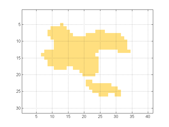
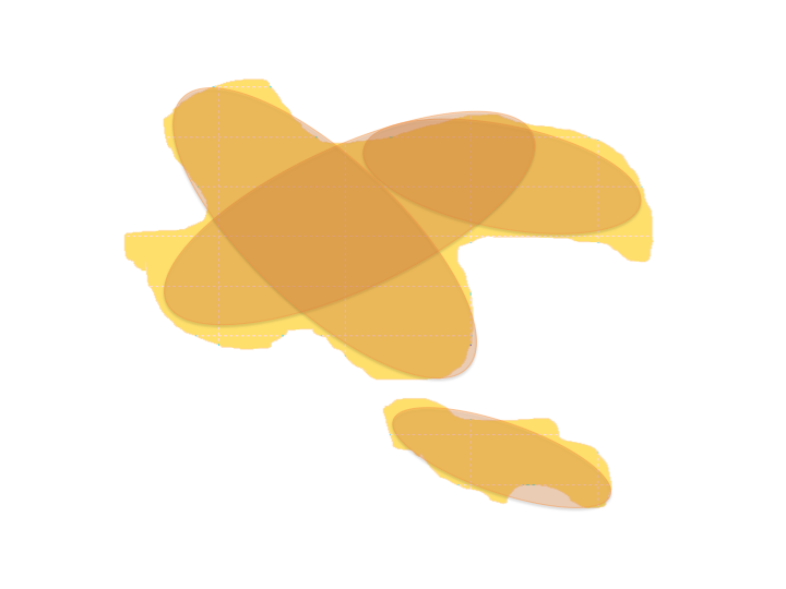
Next, let $\{\hbox{\boldmath$\theta$}_{1},\hbox{\boldmath$\theta$}_{2},\dots,\hbox{\boldmath$\theta$}_{N}\}$ be the set of $N$ high velocity objects, we denote $v_{h}$ the velocity in the homogeneous background and $v_{i}$ the velocity for object $\hbox{\boldmath$\theta$}_{i}$. Because we may have several objects overlapping with each other, the velocity in the overlapping volume has to be defined carefully. In this case, we define the velocity at location $(x,y)$ as the maximum velocity among all objects that include $(x,y)$:

$$V(x,y)=\left\{\begin{array}[]{cc}\displaystyle{\max_{i}}~{}v_{i},&(x,y)\in|{\hbox{\boldmath$\theta$}}_{i}|\\ v_{h},&(x,y)\not\in\overset{N}{\underset{i=1}{\cup}}|{\hbox{\boldmath$\theta$}}_{j}|\end{array}\right.$$ (1)

Obviously the spatial velocity distribution is implicitly determined by the location of objects. We use the notation $V(\hbox{\boldmath$\theta$}_{1},\dots,\hbox{\boldmath$\theta$}_{N})$ to indicate the velocity distribution when we have $N$ objects with parameters $\hbox{\boldmath$\theta$}_{1},\dots,\hbox{\boldmath$\theta$}_{N}$ in the model. Following the same notation, we use $d(\hbox{\boldmath$\theta$}_{i},\hbox{\boldmath$\theta$}_{j})$ to represent the distance between two objects, which is given by:

$$d(\hbox{\boldmath$\theta$}_{i},\hbox{\boldmath$\theta$}_{j})=\min_{\boldsymbol{\mu,\nu}}\|\boldsymbol{\mu}-\boldsymbol{\nu}\|_{2},~{}\boldsymbol{\mu}\in|{\hbox{\boldmath$\theta$}}_{i}|,~{}\boldsymbol{\nu}\in|{\hbox{\boldmath$\theta$}}_{j}|$$ (2)

and the corresponding path is denoted by $\vec{P}({\hbox{\boldmath$\theta$}_{i},\hbox{\boldmath$\theta$}_{j}})$. Obviously, if $\hbox{\boldmath$\theta$}_{i}$ overlaps with $\hbox{\boldmath$\theta$}_{j}$ then $d(\hbox{\boldmath$\theta$}_{i},\hbox{\boldmath$\theta$}_{j})=0$. The same notation can be used for the distance between a point and an object, or between two points, e.g., $d(\hbox{\boldmath$\alpha$},\hbox{\boldmath$\beta$})$ and $\vec{P}({\hbox{\boldmath$\alpha$},\hbox{\boldmath$\beta$}})$ are the distance and path between points $\alpha$ and $\beta$, respectively.

III Forward step

In this paper, we address the problem of identifying high velocity structures in homogeneous background with sparse data. To solve this problem, we need a “forward” model to compute the traveltime for a given velocity model. Then, in the inverse step, a velocity model is estimated by minimizing the mismatch between predicted and measured traveltime data.

Given the velocity model as input, the forward model will compute the corresponding traveltime between transmitter and receiver. We use the mathematical formulation proposed in [4] to calculate the traveltime, where the travel path is defined as the direction of wave-front propagation. Based on Fermat’s principle, the actual travel path is the one with minimum cost time from all possible paths connecting the transmitter and the receiver. The time cost of an arbitrary path $P$ connecting two points $(\hbox{\boldmath$\alpha$},\hbox{\boldmath$\beta$})$ based on velocity model $V$ is defined by the path integral:

$$\tau^{P}(V,\hbox{\boldmath$\alpha$},\hbox{\boldmath$\beta$})=\int_{P}\frac{1}{V(x,y)}dl^{P},~{}\{P_{sart},P_{end}\}=\{\hbox{\boldmath$\alpha$},\hbox{\boldmath$\beta$}\}.$$ (3)

The travel path, $P^{*}$, is defined as the path with minimum time cost $\tau^{*}$. Therefore, we can also define the travel time $\tau^{*}$ between two points $\{\hbox{\boldmath$\alpha$},\hbox{\boldmath$\beta$}\}$ as:

$$\tau^{*}(V,\hbox{\boldmath$\alpha$},\hbox{\boldmath$\beta$}) = \min_{P}\tau^{P}(V,\hbox{\boldmath$\alpha$},\hbox{\boldmath$\beta$})$$ (4)

$$= \min_{P}\int_{P}\frac{1}{V(x,y)}\,dl^{P}.$$

The travel path $P^{*}$ will be:

$$P^{*}(V,\hbox{\boldmath$\alpha$},\hbox{\boldmath$\beta$})=\operatorname*{arg\,min}_{P}~{}\tau^{P}(V,\hbox{\boldmath$\alpha$},\hbox{\boldmath$\beta$}).$$ (5)

Finding the analytic solution for the traveltime $\tau^{*}$ and travel path $P^{*}$ is a classical problem in calculus of variations [8]. Most approaches, including shotgun ray-tracing or fast marching [6, 29, 25] tend to be very computationally intensive due to the frequent update of traveltime in each cell.

III-A Fast travel time/path finding

The object-based model we proposed in Section II is a generic model. Each object can have arbitrary velocity, and the model has the ability to present any velocity distribution. In this paper we use Markov Chain Monte Carlo (MCMC) sampling for reconstruction. Typically Monte Carlo sampling is considered to be too computational expensive for traveltime tomography. The reason is that in each iteration we would need to calculate the traveltime for a new model, and then run a large number iterations to sample the probability space. Thus, it is critical to find a way to calculate the traveltime efficiently.

Since we consider the high contrast velocity case, for simplicity here we assume that all objects have the same velocity, which is much higher than the background velocity, i.e., $v_{1}=v_{2}=\dots=v_{N}$ and $v_{i}\gg v_{h}$. This assumption will not be valid for smooth velocity variation. But for the application we consider, fractured reservoir characterization, the fracture permeability is several orders of magnitude higher than that of the host rocks. With the high velocity contrast assumption, the time spent passing through an object can be ignored, which provides a way to find the fastest travel path by considering the path between objects recursively, thus greatly reducing the computational complexity. We will explain this concept next.

It is well known that the travel path is a straight line in homogeneous medium. We start by considering a simple scenario, where there is only one object in the model. Obviously, there are two possible cases for the travel path, i.e., the travel path may or may not traverse the object. If the path does not traverse the object, the whole path will belong to the homogeneous background, which implies that it must be a straight ray connecting transmitter and receiver. Otherwise, if the path passes through the object, it will be a combination of three parts, corresponding to the paths i) from transmitter to object, ii) inside object and iii) from object to receiver. Each part traverses a constant velocity medium, thus, the travel path must be a combination of line segments.

With the high contrast velocity assumption, the travel time inside the volume $|{\hbox{\boldmath$\theta$}_{1}}|$ is negligible. Thus, the travel path/time through the object must be the “shortest” path from transmitter to $|{\hbox{\boldmath$\theta$}_{1}}|$, a path inside $|{\hbox{\boldmath$\theta$}_{1}}|$ and the “shortest” path from $|{\hbox{\boldmath$\theta$}_{1}}|$ to the receiver, which are all straight lines. We use $\vec{P}(\hbox{\boldmath$\alpha$},\hbox{\boldmath$\gamma$})$, $\vec{P}(\hbox{\boldmath$\gamma$},\hbox{\boldmath$\zeta$})$ and $\vec{P}(\hbox{\boldmath$\gamma$},\hbox{\boldmath$\beta$})$ to denote these lines, where $\hbox{\boldmath$\gamma$},\hbox{\boldmath$\zeta$}$ are the closest points to transmitter $\alpha$, receiver $\beta$ in $|\hbox{\boldmath$\theta$}_{1}|$, which are defined as:

$$\hbox{\boldmath$\gamma$}=\operatorname*{arg\,min}_{\hbox{\boldmath$\gamma$}}\|\hbox{\boldmath$\alpha$}-\hbox{\boldmath$\gamma$}\|, ~{}\hbox{\boldmath$\zeta$}=\operatorname*{arg\,min}_{\hbox{\boldmath$\zeta$}}\|\hbox{\boldmath$\beta$}-\hbox{\boldmath$\zeta$}\|$$ (6)

$$\text{where}~{}\{\hbox{\boldmath$\gamma$},\hbox{\boldmath$\zeta$}\}\in|\hbox{\boldmath$\theta$}_{1}|.$$

This travel path can be denoted as $\hbox{\boldmath$\alpha$}-\hbox{\boldmath$\theta$}_{1}-\hbox{\boldmath$\beta$}$ which describes the order in which the objects are traversed. If we assume that the traveltime inside the object is negligible, the traveltime function in the one-object case becomes

$$\tau^{*}(V(\hbox{\boldmath$\theta$}_{1}),\hbox{\boldmath$\alpha$},\hbox{\boldmath$\beta$})=\min\left\{\begin{array}[]{c}1/v_{h}\cdot{d(\hbox{\boldmath$\alpha$},\hbox{\boldmath$\beta$})}\\ 1/v_{h}\cdot(~{}d(\hbox{\boldmath$\alpha$},\hbox{\boldmath$\theta$}_{1})+d(\hbox{\boldmath$\theta$}_{1},\hbox{\boldmath$\beta$})~{})\end{array}\right.$$ (7)

Next, we consider the two object case $N=2$. Obviously, there are three possible cases for the travel path, namely, i) not traversing any object, ii) traversing exactly one object, or iii) traversing both objects. From (7) we know how to compute the travel path/time in the cases when a single object is traversed. Thus, we only need to analyze how to compute the paths which pass through both objects, $|{\hbox{\boldmath$\theta$}}_{1}|$ and $|{\hbox{\boldmath$\theta$}}_{2}|$, in different orders, and then compare them with the previous results.

We notice that the path $\hbox{\boldmath$\alpha$}-\hbox{\boldmath$\theta$}_{1}-\hbox{\boldmath$\theta$}_{2}-\hbox{\boldmath$\beta$}$ includes the shortest paths from $\alpha$ to object $\hbox{\boldmath$\theta$}_{1}$, from object $\hbox{\boldmath$\theta$}_{1}$ to object $\hbox{\boldmath$\theta$}_{2}$, and from object $\hbox{\boldmath$\theta$}_{2}$ to $\beta$. Similar to (7), the corresponding travel time will be $1/v_{h}\cdot(~{}d(\hbox{\boldmath$\alpha$},\hbox{\boldmath$\theta$}_{1})+d(\hbox{\boldmath$\theta$}_{1},\hbox{\boldmath$\theta$}_{2})+d(\hbox{\boldmath$\theta$}_{2},\hbox{\boldmath$\beta$})~{})$, where $d(\hbox{\boldmath$\alpha$},\hbox{\boldmath$\theta$}_{1})$ has been calculated in the previous step in order to evaluate the path $\hbox{\boldmath$\alpha$}-\hbox{\boldmath$\theta$}_{1}-\hbox{\boldmath$\beta$}$. Thus, $d(\hbox{\boldmath$\theta$}_{1},\hbox{\boldmath$\theta$}_{2})$ and $d(\hbox{\boldmath$\theta$}_{2},\hbox{\boldmath$\beta$})$ are the only new terms to be calculated. A similar result also holds for $\hbox{\boldmath$\alpha$}-\hbox{\boldmath$\theta$}_{2}-\hbox{\boldmath$\theta$}_{1}-\hbox{\boldmath$\beta$}$, where only $d(\hbox{\boldmath$\alpha$},\hbox{\boldmath$\theta$}_{2})$ and $d(\hbox{\boldmath$\theta$}_{2},\hbox{\boldmath$\theta$}_{1})$ would be needed. Note that $d(\hbox{\boldmath$\theta$}_{2},\hbox{\boldmath$\theta$}_{1})=d(\hbox{\boldmath$\theta$}_{1},\hbox{\boldmath$\theta$}_{2})$ so that this distance does not need to be recomputed.

In summary, given two objects in the velocity model the traveltime can be computed as (again the traveltime inside objects is considered negligible):

$$\tau^{*}(V(\hbox{\boldmath$\theta$}_{1},\hbox{\boldmath$\theta$}_{2}),\hbox{\boldmath$\alpha$},\hbox{\boldmath$\beta$}) =$$

$$1/v_{h}\cdot\min \left\{\begin{array}[]{c}d(\hbox{\boldmath$\alpha$},\hbox{\boldmath$\beta$})\\ d(\hbox{\boldmath$\alpha$},\hbox{\boldmath$\theta$}_{1})+d(\hbox{\boldmath$\theta$}_{1},\hbox{\boldmath$\beta$})\\ d(\hbox{\boldmath$\alpha$},\hbox{\boldmath$\theta$}_{2})+d(\hbox{\boldmath$\theta$}_{2},\hbox{\boldmath$\beta$})\\ d(\hbox{\boldmath$\alpha$},\hbox{\boldmath$\theta$}_{1})+d(\hbox{\boldmath$\theta$}_{1},\hbox{\boldmath$\theta$}_{2})+d(\hbox{\boldmath$\theta$}_{2},\hbox{\boldmath$\beta$})\\ d(\hbox{\boldmath$\alpha$},\hbox{\boldmath$\theta$}_{2})+d(\hbox{\boldmath$\theta$}_{2},\hbox{\boldmath$\theta$}_{1})+d(\hbox{\boldmath$\theta$}_{1},\hbox{\boldmath$\beta$})\end{array}\right.\ldotp$$ (13)

Note that we need to compute and compare $5$ different possible paths in the 2-object case. But two of them $\{d(\hbox{\boldmath$\alpha$},\hbox{\boldmath$\theta$}_{1})+d(\hbox{\boldmath$\theta$}_{1},\hbox{\boldmath$\theta$}_{2})+d(\hbox{\boldmath$\theta$}_{2},\hbox{\boldmath$\beta$}),~{}d(\hbox{\boldmath$\alpha$},\hbox{\boldmath$\theta$}_{2})+d(\hbox{\boldmath$\theta$}_{2},\hbox{\boldmath$\beta$})\}$ are actually trying to find the fastest path from $\alpha$ to object $\hbox{\boldmath$\theta$}_{2}$, then travel from $\hbox{\boldmath$\theta$}_{2}$ to $\beta$. Thus, Equation (III-A) can be reformulated as

$$\tau^{*}(V(\hbox{\boldmath$\theta$}_{1},\hbox{\boldmath$\theta$}_{2}), \hbox{\boldmath$\alpha$},\hbox{\boldmath$\beta$})=$$

$$\min \left\{\begin{array}[]{c}1/v_{h}\cdot d(\hbox{\boldmath$\alpha$},\hbox{\boldmath$\beta$})\\ \tau^{*}(V(\hbox{\boldmath$\theta$}_{1},\hbox{\boldmath$\theta$}_{2}),\hbox{\boldmath$\alpha$},\hbox{\boldmath$\theta$}_{1})+1/v_{h}\cdot d(\hbox{\boldmath$\theta$}_{1},\hbox{\boldmath$\beta$})\\ \tau^{*}(V(\hbox{\boldmath$\theta$}_{1},\hbox{\boldmath$\theta$}_{2}),\hbox{\boldmath$\alpha$},\hbox{\boldmath$\theta$}_{2})+1/v_{h}\cdot d(\hbox{\boldmath$\theta$}_{2},\hbox{\boldmath$\beta$})\\ \end{array}\right.\ldotp$$ (17)

where

$$\tau^{*}(V(\hbox{\boldmath$\theta$}_{1},\hbox{\boldmath$\theta$}_{2}),\hbox{\boldmath$\alpha$},\hbox{\boldmath$\theta$}_{1})=1/v_{h}\cdot\min\left\{\begin{array}[]{c}d(\hbox{\boldmath$\alpha$},\hbox{\boldmath$\theta$}_{1})\\ d(\hbox{\boldmath$\alpha$},\hbox{\boldmath$\theta$}_{2})+d(\hbox{\boldmath$\theta$}_{2},\hbox{\boldmath$\theta$}_{1})\end{array}\right.\ldotp$$ (18)

It is obvious that if we have $2$ objects, the traveltime can be computed by comparing the fastest path from transmitter to each object $\hbox{\boldmath$\theta$}_{i}$. Equation (III-A) can be extended to the case with $N$ objects:

$$\tau^{*}(V(\hbox{\boldmath$\theta$}_{1},\dots,\hbox{\boldmath$\theta$}_{N}),\hbox{\boldmath$\alpha$},\hbox{\boldmath$\beta$})=$$

$$\min\left\{\begin{array}[]{c}1/v_{h}\cdot d(\hbox{\boldmath$\alpha$},\hbox{\boldmath$\beta$})\\ \tau^{*}(V(\hbox{\boldmath$\theta$}_{1},\dots,\hbox{\boldmath$\theta$}_{N}),\hbox{\boldmath$\alpha$},\hbox{\boldmath$\theta$}_{1})+1/v_{h}\cdot d(\hbox{\boldmath$\theta$}_{1},\hbox{\boldmath$\beta$})\\ \vdots\\ \tau^{*}(V(\hbox{\boldmath$\theta$}_{1},\dots,\hbox{\boldmath$\theta$}_{N}),\hbox{\boldmath$\alpha$},\hbox{\boldmath$\theta$}_{N})+1/v_{h}\cdot d(\hbox{\boldmath$\theta$}_{N},\hbox{\boldmath$\beta$})\\ \end{array}\right.\ldotp$$ (23)

and

$$\tau^{*}(V(\hbox{\boldmath$\theta$}_{1},\dots,\hbox{\boldmath$\theta$}_{N}),\hbox{\boldmath$\alpha$},\hbox{\boldmath$\theta$}_{i})=$$

$$\min\left\{\begin{array}[]{c}1/v_{h}\cdot d(\hbox{\boldmath$\alpha$},\hbox{\boldmath$\theta$}_{i})\\ \tau^{*}(V(\hbox{\boldmath$\theta$}_{1},\dots,\hbox{\boldmath$\theta$}_{N}),\hbox{\boldmath$\alpha$},\hbox{\boldmath$\theta$}_{1})+1/v_{h}\cdot d(\hbox{\boldmath$\theta$}_{1},\hbox{\boldmath$\theta$}_{i})\\ \vdots\\ \tau^{*}(V(\hbox{\boldmath$\theta$}_{1},\dots,\hbox{\boldmath$\theta$}_{N}),\hbox{\boldmath$\alpha$},\hbox{\boldmath$\theta$}_{N})+1/v_{h}\cdot d(\hbox{\boldmath$\theta$}_{N},\hbox{\boldmath$\theta$}_{i})\end{array}\right.\ldotp$$ (28)

Note that in equation (III-A), the calculations of traveltime seem to be correlated with each other and hard to compute. However, we notice that the distances between objects are always “non-negative”, which provides us an opportunity to simplify the min operation in the calculation.

To show how this property can dramatically simplify the calculation, we start the calculation by finding the “closest” object $\hbox{\boldmath$\theta$}_{k_{1}}$ from $\alpha$. This can be found immediately by comparing the distance from transmitter to all objects:

$$\hbox{\boldmath$\theta$}_{k_{1}}=\underset{\hbox{\boldmath$\theta$}_{i}}{\operatorname*{arg\,min}}~{}d(\hbox{\boldmath$\alpha$},\hbox{\boldmath$\theta$}_{i})$$ (29)

and the traveltime will be:

$$\tau^{*}(V(\hbox{\boldmath$\theta$}_{1},\dots,\hbox{\boldmath$\theta$}_{N}),\hbox{\boldmath$\alpha$},\hbox{\boldmath$\theta$}_{k_{1}})=1/v_{h}\cdot d(\hbox{\boldmath$\alpha$},\hbox{\boldmath$\theta$}_{k_{1}})$$ (30)

Why does the travel path to the closest object only contain the direct path from transmitter? It can be easily proved by the following statements. Assume that $\hbox{\boldmath$\theta$}_{k_{1}}$ is the closest object, and the travel path is not the direct path, i.e., the travel time/path is a combination of the path through another object $\hbox{\boldmath$\theta$}_{j}$. In other words, $\tau^{*}(V(\hbox{\boldmath$\theta$}_{1},\dots,\hbox{\boldmath$\theta$}_{N}),\hbox{\boldmath$\alpha$},\hbox{\boldmath$\theta$}_{k_{1}})=\tau^{*}(V(\hbox{\boldmath$\theta$}_{1},\dots,\hbox{\boldmath$\theta$}_{N}),\hbox{\boldmath$\alpha$},\hbox{\boldmath$\theta$}_{j})+1/v_{h}\cdot d(\hbox{\boldmath$\theta$}_{k_{1}},\hbox{\boldmath$\theta$}_{j})$. But the distance between objects is always greater than zero, $d(\hbox{\boldmath$\theta$}_{k_{1}},\hbox{\boldmath$\theta$}_{j})\geq 0$, therefore $\tau^{*}(V(\hbox{\boldmath$\theta$}_{1},\dots,\hbox{\boldmath$\theta$}_{N}),\hbox{\boldmath$\alpha$},\hbox{\boldmath$\theta$}_{k_{1}})\geq\tau^{*}(V(\hbox{\boldmath$\theta$}_{1},\dots,\hbox{\boldmath$\theta$}_{N}),\hbox{\boldmath$\alpha$},\hbox{\boldmath$\theta$}_{j})$. This implies that another object $\hbox{\boldmath$\theta$}_{j}$ has shorter traveltime than $\hbox{\boldmath$\theta$}_{k_{1}}$, which contradicts the assumption and completes our proof.

With the same concept, we can find the second “closest” (shortest traveltime) object by considering the path traverses through $\hbox{\boldmath$\theta$}_{k_{1}}$. The cost time to each object $\hbox{\boldmath$\theta$}_{i}$ through $\hbox{\boldmath$\theta$}_{k_{1}}$ will be:

$$\tau(V(\hbox{\boldmath$\theta$}_{1}, \dots,\hbox{\boldmath$\theta$}_{N}),\hbox{\boldmath$\alpha$},\hbox{\boldmath$\theta$}_{i})=$$

$$\min \left\{\begin{array}[]{c}1/v_{h}\cdot d(\hbox{\boldmath$\alpha$},\hbox{\boldmath$\theta$}_{i})\\ \tau^{*}(V(\hbox{\boldmath$\theta$}_{1},\dots,\hbox{\boldmath$\theta$}_{N}),\hbox{\boldmath$\alpha$},\hbox{\boldmath$\theta$}_{k_{1}})+1/v_{h}\cdot d(\hbox{\boldmath$\theta$}_{k_{1}},\hbox{\boldmath$\theta$}_{i})\\ \end{array}\right.\ldotp$$ (33)

Then the second “closest” object $\hbox{\boldmath$\theta$}_{k_{2}}$ can be selected with the minimum of cost time among these objects.

$$\tau^{*}(V(\hbox{\boldmath$\theta$}_{1},\dots,\hbox{\boldmath$\theta$}_{N}),\hbox{\boldmath$\alpha$},\hbox{\boldmath$\theta$}_{k_{2}})=\displaystyle{\min_{i,i\neq k_{1}}}\tau(V(\hbox{\boldmath$\theta$}_{1},\dots,\hbox{\boldmath$\theta$}_{N}),\hbox{\boldmath$\alpha$},\hbox{\boldmath$\theta$}_{i})$$ (34)

Following this procedure, after $n$ iterations we can find the $n$-th “closest” object. This process is very similar to the fast marching method to solve the Eikonal problem, which never backtracks over previously evaluated grid points. In the next section, we will use this concept and introduce an efficient algorithm to compute the travel path.

III-B Dijkstra path finding

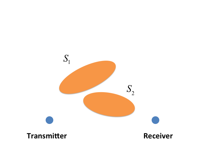
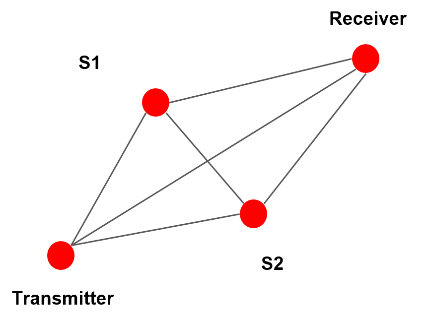
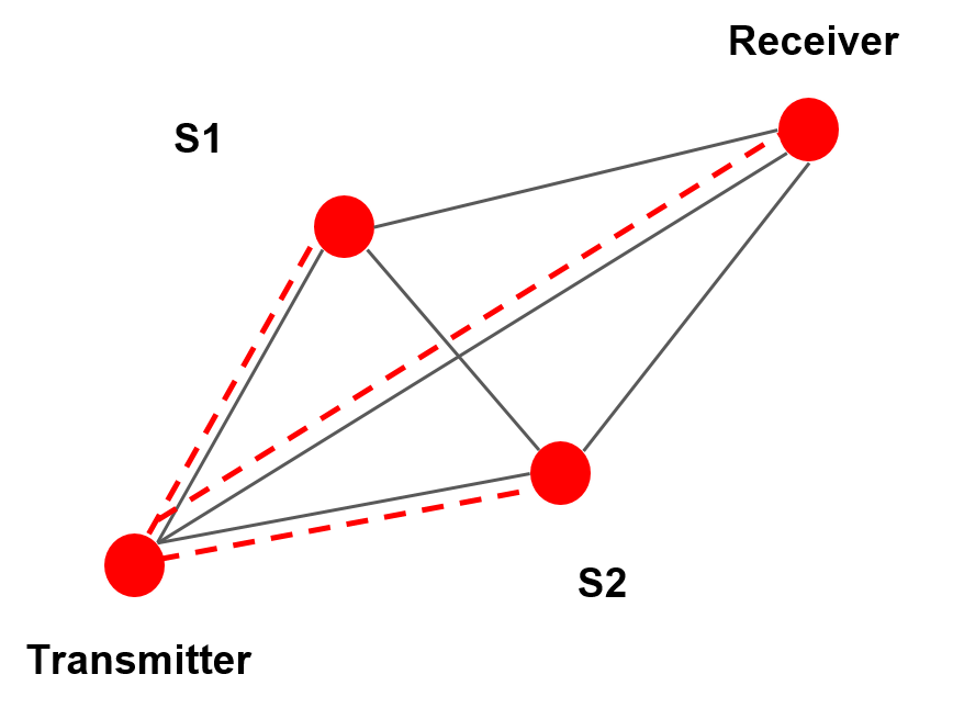
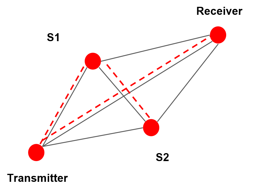
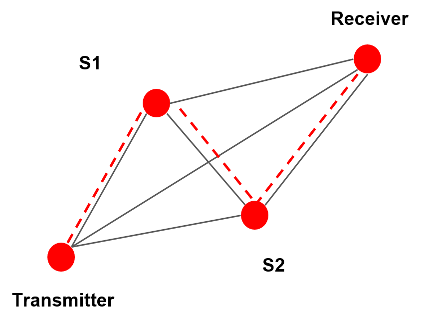
Note that in  (III-A), as well as in more general cases with more objects, the traveltime is obtained by comparing different possible paths. Assuming that we would like to find the traveltime from the source to the destination, the fastest path may traverse one or more objects; which objects and in which order they are traversed is not known. From the previous discussion, we know the fastest path from transmitter to receiver can be found by iteratively finding the “closest” object. To solve this problem systemically, we construct a graph $G=(v,e)$ where each node represents an object, and additional source and destination nodes are defined for the transmitter and receiver. This graph is fully connected with N+2 nodes, and the edge weight between the nodes is the distance between the corresponding objects defined in (2) (sources, destinations or objects, see Fig. 2).

After constructing the graph and computing the edge weight (i.e., the pairwise distance between objects), we apply the Dijkstra algorithm to find the shortest distance from source (transmitter) node to destination (receiver) node. The Dijkstra algorithm iteratively construct a shortest-path tree from the source node to every other node in the graph. We demonstrate the construction of shortest-path tree and update of distance metric by considering an example with two objects. The geometrical location of objects and the corresponding graph are shown in Fig. 2, while the distance metric updates are demonstrated in Fig. 3. In the initial stage, the traveltime from source $\alpha$ to all other nodes is unknown, thus the metric on all other nodes is set to infinity. Then, in the first step the metric is updated by the direct path from $\alpha$ to all other nodes, shown in Fig. 3(a). Node $S_{1}$ is selected as the “closest” object, and we update the metric for neighbors of $S_{1}$ by comparing the tentative distance and the recorded distance. For instance, node $S_{1}$ has distance metric $3$ and the edge between $S_{1},S_{2}$ is equal to $1$, thus the “tentative” path to $S_{2}$ has cost $v(S_{1})+e(S_{1},S_{2})=4$. Then we compare this new tentative path with the original cost and choose the minimum. Thus, the metric in node $S_{2}$ is updated to $4$ and node $\beta$ is updated to $8$. By iteratively selecting the closest node, the fastest path to $\beta$ is eventually found with the path $\alpha-S_{1}-S_{2}-\beta$.

(a)

(b)

Figure 2: Example of graph representation of an object model. (a) Geometrical locations of the objects (b) Graph model, where the edge weight is the geometrical distance between objects.

Algorithm 1 Dijkstra algorithm for path tracking

dist[$s$] $\leftarrow 0$ $\triangleright$ distance to source is zero

for all $v\in{\bf V}\setminus s$ do $\triangleright$ initialization

    dist[$v$] $\leftarrow\infty$

${\bf S}=\emptyset$ $\triangleright$ initially the set of visited vertices is empty

${\bf Q}\leftarrow{\bf G}$

while ${\bf Q}\neq\emptyset$ do

    $u\mathrel{\mathop{:}}=v\in{\bf Q}$ with minimum dist$[v]$

    ${\bf S}\leftarrow{\bf S}\cup u$

    ${\bf Q}\leftarrow{\bf Q}\setminus u$

    for  all $v\in$ neighbor[$u$] and $v\in{\bf Q}$ do

         if dist$[u]+e(u,v)\leq$ dist$[v]$ then

             dist$[v]$ $\leftarrow$ dist$[u]+e(u,v)$              

(a)

(b)

(c)

Figure 3: Example of the Dijkstra algorithm to find the travel path. (a) After initialization, the cost to each node will be the direct path. (b) The cost and path to $S_{2}$ are updated by the path through $S_{1}$. (c) The final result. The traveltime is determined by the path through $S_{1}$ and $S_{2}$.

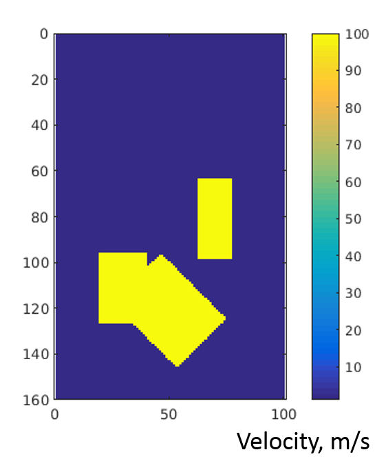
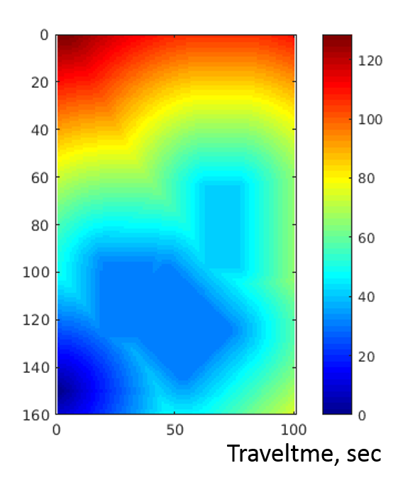
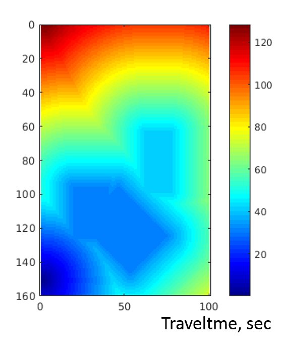
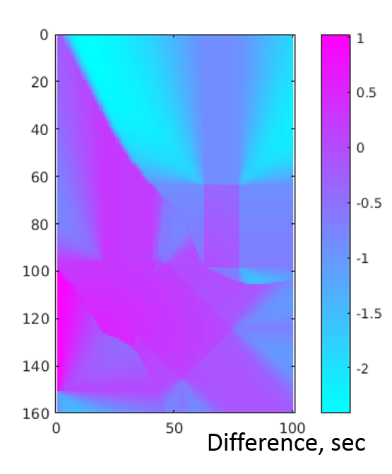
To validate our method, we build a 2D velocity model with size $100~{}\text{m}\times 160~{}\text{m}$ and velocity equal to $1~{}m/s$ in the background and $100~{}m/s$ in the objects. The transmitter is located in the lower left corner of the model and we calculate the “distance map”, representing the traveltime from the transmitter to each point. In Fig. 4, we show the results from our approach and the well know fast marching method [24, 11] which uses rectangular cells with size $1\text{m}\times 1\text{m}$. The calculated distance map from our approach is very close to that obtained from fast marching method, but our method has much faster computational time. The reason is that both methods convert the travel path finding into a shortest path problem in graph. However, instead of using the rectangular cells to represent the velocity model, our approach uses “objects” to represent the velocity model which reduces the number of nodes in the graph from $100\times 100$ (number of cells) to $4$. When running the Dijkstra algorithm to find the shortest path on the graph (while the simplest implementation has computational complexity $O(|V|^{2})$ and memory requirement $O(|V|)$), the cost time drops from $O(10,000^{2})$ to $O(4^{2})$.

(a)

(b)

(c)

(d)

Figure 4: Distance map: the traveltime from transmitter in $(1,150)$ (a) Base velocity model, where the background velocity is $1~{}m/s$ and object is $100~{}m/s$ (b) Result obtained with our approach (c) Result from fast marching method (d) Difference between two approaches. Note most of the differences are within $5\%$.

IV Inverse Problem Solution

In the forward step we just presented, we can predict the traveltime when the velocity model is given. Next, for the inverse step the goal is to estimate the velocity model when the traveltime data is observed. With limited measured data, this becomes an ill-posed inverse problem and the solution may not be unique. Since multiple solutions may exist, rather than selecting a single model as the output of our algorithm, we formulate it as a statistical inference problem and estimate the probability distribution in the velocity model parameter space. We start this section by introducing some notations.

IV-A Notation

The input data is obtained by measuring the traveltime between the set of transmitters $\mathcal{A}=\{\hbox{\boldmath$\alpha$}_{1},\dots,\hbox{\boldmath$\alpha$}_{p}\}$ and receivers $\mathcal{B}=\{\hbox{\boldmath$\beta$}_{1},\dots,\hbox{\boldmath$\beta$}_{q}\}$. We denote the measured traveltime for all transmitter-receiver pairs $(\hbox{\boldmath$\alpha$}_{i},\hbox{\boldmath$\beta$}_{j})$ as a vector ${\bf t}=\{t_{1},\dots,t_{n}\}$, where $n=p\cdot q$. Assuming that there are $N$ objects in the velocity model, we can group all parameters and define a vector of model parameters, $\boldsymbol{\Theta}=\{\hbox{\boldmath$\theta$}_{1},\dots,\hbox{\boldmath$\theta$}_{N}\}$, so that the velocity model $V(\hbox{\boldmath$\theta$}_{1},\dots,\hbox{\boldmath$\theta$}_{N})$ can be represented simply by $V(\boldsymbol{\Theta})$.

The predicted traveltime, based on the velocity model parameters $\boldsymbol{\Theta}$, will be a vector function ${\bf T}(\boldsymbol{\Theta},\mathcal{A},\mathcal{B})$ representing the traveltime between each pair of transmitters and receivers:

$${\bf T}(\boldsymbol{\Theta},\mathcal{A},\mathcal{B})=(T_{1}(\boldsymbol{\Theta},\mathcal{A},\mathcal{B}),\dots,T_{n}(\boldsymbol{\Theta},\mathcal{A},\mathcal{B})),$$ (35)

where

$$\left\{~{}\ \begin{matrix}T_{1}(\boldsymbol{\Theta},\mathcal{A},\mathcal{B})&=&\tau^{*}(V(\hbox{\boldmath$\theta$}_{1},\dots,\hbox{\boldmath$\theta$}_{N}),\hbox{\boldmath$\alpha$}_{1},\hbox{\boldmath$\beta$}_{1})\\ &\vdots&\\ T_{n}(\boldsymbol{\Theta},\mathcal{A},\mathcal{B})&=&\tau^{*}(V(\hbox{\boldmath$\theta$}_{1},\dots,\hbox{\boldmath$\theta$}_{N}),\hbox{\boldmath$\alpha$}_{p},\hbox{\boldmath$\beta$}_{q}).\\ \end{matrix}\right.$$ (36)

IV-B Posterior Probability

To recover model parameters that match the measured traveltime, we use the quadratic data-fitting error between the predicted traveltime and the measurements as the cost function:

$$E(\boldsymbol{\Theta})=[{\bf t}-{\bf T}(\boldsymbol{\Theta},\mathcal{A},\mathcal{B})]^{t}{\bf C}_{t}^{-1}[{\bf t}-{\bf T}(\boldsymbol{\Theta},\mathcal{A},\mathcal{B})]$$ (37)

where ${\bf C}_{t}$ is the covariance matrix of measured traveltime. If the measurement noise is an independent and identically distributed (i.i.d.) Gaussian random variable, the covariance matrix will be proportional to an identity matrix, ${\bf C}_{t}=\rho\cdot{\bf I}$, and the cost function can be simplified as $E(\boldsymbol{\Theta})=\|{\bf t}-{\bf T}(\boldsymbol{\Theta},\mathcal{A},\mathcal{B})\|^{2}$. Then, the likelihood function, which is the probability density of the measurement ${\bf t}$ given the model $\boldsymbol{\Theta}$ will be:

$$f({\bf t}|\boldsymbol{\Theta})=\frac{1}{Z}\cdot\text{exp}[-E(\boldsymbol{\Theta})/2]$$ (38)

where $Z$ is a normalization constant. We use the Bayesian approach to combine the prior knowledge and the measurements. So that the posterior probability density $f(\boldsymbol{\Theta}|{\bf t})$ is defined by Bayes rule:

$$f(\boldsymbol{\Theta}|{\bf t}) =f({\bf t}|\boldsymbol{\Theta})\cdot\frac{f(\boldsymbol{\Theta})}{f({\bf t})}$$ (39)

$$=k\cdot f({\bf t}|\boldsymbol{\Theta})\cdot f(\boldsymbol{\Theta})$$ (40)

where $f(\boldsymbol{\Theta})$ is the prior probability density of model $\boldsymbol{\Theta}$, and $k$ is a normalization constant.

We can use maximum a posteriori (MAP) estimation on (39) to estimate a single model, but when the measured traveltime is noisy and the number of measurements is limited, providing one single model may not be the best way to explain the data. In this case, it is highly likely that there will be multiple models that reach the minimum of the cost function. In the next section, we use the Hybrid Monte Carlo (HMC) method to sample the probability density and use the resulting samples to generate an “ensemble” model to explain the data.

IV-C Proposed algorithm

Because the probability density function is defined by the cost function, and the cost function of any model can be calculated based on the mismatch between the prediction of traveltime function and measured data, we can easily evaluate the probability at any point in model parameter space. However in a high dimensional space, it is not easy to draw samples from a given probability distribution [16]. For example, a naive approach would be to divide the whole parameter space into uniform grids, evaluating the probability in every point and drawing the samples proportional to the probability. However, the number of points to be visited grows exponentially with the dimensions of the space. If a velocity model has $3$ objects, and each object requires $5$ parameters to describe its properties, this model will have $15$ parameters. If we divide each parameter into $10$ grids, we need to evaluate the probability in $10^{15}$ different points, which clearly makes this uniform probing approach impractical.

The Metropolis method [10] is a widely used approach to generate samples from a high-dimensional distribution. It is an example of Markov chain Monte Carlo method (MCMC), where samples are generated by random walk and we decide to accept them or reject them based on target density. Unlike importance sampling or rejection sampling, it does not suffer as much from the “curse of dimensionality”. However, due to the random walk behavior in the Metropolis algorithm, it could take a long time to converge to the target density. To overcome this problem, we use the Hybrid Monte Carlo (HMC) algorithm [19] which explores the parameter space more efficiently and speeds up the sampling process.

IV-C1 Hamiltonian Dynamics

The Hybrid Monte Carlo is a Metropolis method which simulates Hamiltonian dynamics to draw new samples. In HMC, we define a dynamical system where the model parameter vector $\boldsymbol{\Theta}$ is augmented by a momentum vector ${\bf p}$, where $\boldsymbol{\Theta},{\bf p}$ have the same size and ${\bf p}$ is randomly chosen. The total energy $H(\boldsymbol{\Theta},{\bf p})$ of the dynamical system is defined as the sum of “kinetic energy” and the “potential energy”, where the “potential energy” is equal to the error function $E(\boldsymbol{\Theta})$ and the “kinetic energy” is given by $K({\bf p})=\|{\bf p}\|^{2}/2$. Thus, $H(\boldsymbol{\Theta},{\bf p})=E(\boldsymbol{\Theta})+K({\bf p})$ and the change of state is determined by the Hamiltonian mechanics:

$$\frac{\partial{\boldsymbol{\Theta}}}{\partial t} ={\bf p},$$ (41a)

$$\frac{\partial{{\bf p}}}{\partial t} =\frac{-\partial{E(\boldsymbol{\Theta})}}{\partial{\boldsymbol{\Theta}}}$$ (41b)

To generate samples for model parameters, we choose a random momentum and calculate the change of parameters by solving the Hamiltonian dynamics in (41). This process can be viewed as sampling from the joint density

$$P_{H}(\boldsymbol{\Theta},{\bf p}) =\frac{1}{Z_{H}}\text{exp}[-H(\boldsymbol{\Theta},{\bf p})]$$

$$=\frac{1}{Z_{H}}\text{exp}[-E(\boldsymbol{\Theta})]\text{exp}[-K({\bf p})]$$ (42)

Because the density is separable, $P_{H}(\boldsymbol{\Theta},{\bf p})=P(\boldsymbol{\Theta})P({\bf p})$, we can ignore the momentum variable and obtain the samples $\boldsymbol{\Theta}^{(t)}$ that are asymptotically generated from $P(\boldsymbol{\Theta})$.

IV-C2 Leap Frog Algorithm

To simulate the Hamiltonian dynamics in discrete time, we use the “Verlet / Leap-Frog” algorithm [27] to maintain the time reversal symmetry. Starting from the Taylor’s expansion, we can write the discretized $\boldsymbol{\Theta}_{n}$ as:

$$\boldsymbol{\Theta}_{n+1}=\boldsymbol{\Theta}_{n}+\Delta_{t}\boldsymbol{\Theta}^{{}^{\prime}}_{n}+\frac{1}{2}(\Delta_{t})^{2}\boldsymbol{\Theta}^{{}^{\prime\prime}}_{n}+\frac{1}{6}(\Delta_{t})^{3}\boldsymbol{\Theta}^{{}^{\prime\prime\prime}}_{n}+O(\Delta_{t}^{4})$$

$$\boldsymbol{\Theta}_{n-1}=\boldsymbol{\Theta}_{n}-\Delta_{t}\boldsymbol{\Theta}^{{}^{\prime}}_{n}+\frac{1}{2}(\Delta_{t})^{2}\boldsymbol{\Theta}^{{}^{\prime\prime}}_{n}-\frac{1}{6}(\Delta_{t})^{3}\boldsymbol{\Theta}^{{}^{\prime\prime\prime}}_{n}+O(\Delta_{t}^{4})$$

By adding them together, we have the following equation:

$$\boldsymbol{\Theta}_{n+1}=2\boldsymbol{\Theta}_{n}-\boldsymbol{\Theta}_{n-1}+(\Delta_{t})^{2}\boldsymbol{\Theta}^{{}^{\prime\prime}}_{n}+O(\Delta_{t}^{4})$$ (43)

And we define the discrete ${\bf p}_{n}$ and $\boldsymbol{\Theta}^{{}^{\prime\prime}}_{n}$ in equation (41):

$${\bf p}_{n-\frac{1}{2}} =(\boldsymbol{\Theta}_{n}-\boldsymbol{\Theta}_{n-1})/\Delta_{t}$$ (44a)

$$\boldsymbol{\Theta}^{{}^{\prime\prime}}_{n} =({\bf p}_{n+\frac{1}{2}}-{\bf p}_{n-\frac{1}{2}})/\Delta_{t}$$ (44b)

Substituting (43) into (44), it becomes

$$\boldsymbol{\Theta}_{n+1} =\boldsymbol{\Theta}_{n}+\Delta_{t}({\bf p}_{n-\frac{1}{2}}+\Delta_{t}\boldsymbol{\Theta}^{{}^{\prime\prime}}_{n})+O(\Delta_{t}^{4})$$

$$=\boldsymbol{\Theta}_{n}+\Delta_{t}\cdot{\bf p}_{n+\frac{1}{2}}+O(\Delta_{t}^{4})$$ (45)

Thus we have the Leap-frog algorithm for simulating the discrete Hamiltonian dynamics:

$${\bf p}_{n+\frac{1}{2}} ={\bf p}_{n}-\frac{\Delta_{t}}{2}\cdot\left.\frac{\partial E(\boldsymbol{\Theta})}{\partial\boldsymbol{\Theta}}\right|_{\boldsymbol{\Theta}_{n}}$$ (46a)

$$\boldsymbol{\Theta}_{n+1} =\boldsymbol{\Theta}_{n}+\Delta_{t}\cdot{\bf p}_{n+\frac{1}{2}}$$ (46b)

$${\bf p}_{n+1} ={\bf p}_{n+\frac{1}{2}}-\frac{\Delta_{t}}{2}\cdot\left.\frac{\partial E(\boldsymbol{\Theta})}{\partial\boldsymbol{\Theta}}\right|_{\boldsymbol{\Theta}_{n+1}}$$ (46c)

IV-C3 Accept / Reject Rules

After simulating the Hamiltonian dynamics for $n$ leap-frog steps, we will reach a new state from $\boldsymbol{\Theta}$ to $\boldsymbol{\Theta^{*}}$. Then we use the Metropolis rule to decide if we should accept the new state or stay in the current state. The new state is accepted with probability:

$$P_{\text{accept}}=min\left(1,\frac{\text{exp}(-H(\boldsymbol{\Theta^{*}},{\bf p}^{*}))}{\text{exp}(-H(\boldsymbol{\Theta},{\bf p}))}\right)$$ (47)

If the simulation of the Hamiltonian dynamics is perfect, it will preserve the total energy $H(\boldsymbol{\Theta},{\bf p})$ and new state is always accepted. However, due to the finite step size $\Delta t$ the conservation of total energy is not guaranteed. Thus, the rejection rule in (47) makes sure that the samples are coming from the target joint density $P_{H}(\boldsymbol{\Theta},{\bf p})$.

$\boldsymbol{\Theta}=\boldsymbol{\Theta}_{init}$ $\triangleright$ Initialize model parameters

for $l=1:L$ do $\triangleright$ Repeat the simulation for L times

    ${\bf g}=\nabla E(\boldsymbol{\Theta}),~{}E=E(\boldsymbol{\Theta})$

    ${\bf p}\leftarrow$ randn( size($\boldsymbol{\Theta}$) )

    $H={\bf p}^{t}{\bf p}/2+E$

    $\boldsymbol{\Theta}_{new}=\boldsymbol{\Theta},~{}{\bf g}_{new}={\bf g}$

    for $t=1:T$ do $\triangleright$ Use “leapfrog” to simulate

         ${\bf p}={\bf p}-{\Delta t}/2\cdot{\bf g}_{new}$

         $\boldsymbol{\Theta}_{new}=\boldsymbol{\Theta}_{new}+\Delta t\cdot{\bf p}$

         ${\bf g}_{new}=\nabla E(\boldsymbol{\Theta}_{new})$

         ${\bf p}={\bf p}-{\Delta t}/2\cdot{\bf g}_{new}$     

    $E_{new}=E(\boldsymbol{\Theta}_{new})$

    $H_{new}={\bf p}^{t}{\bf p}/2+E_{new}$

    $\Delta H=H_{new}-H$ $\triangleright$ Accept sample by Metropolis rule

    if $\Delta H<0$ then

         $\boldsymbol{\Theta}=\boldsymbol{\Theta}_{new}$

    else

         if $\text{exp}(-\Delta H)\geq\text{rand()}$ then

             $\boldsymbol{\Theta}=\boldsymbol{\Theta}_{new}$              

Algorithm 2 Hamiltonian Monte Carlo method

V Simulation Results

To validate our approach, we run simulations on a model that contains a high velocity structure in the homogeneous background. The model size is $100$ m by $160$ m, where the transmitters and receivers are placed on the boundary with equal spacing. The synthetic measured traveltime data is generated by the fast marching method (FMM) on a grid-based model with cell size $1\text{m}\times 1\text{m}$, where the ground truth velocity distribution has a high velocity structure equal to $100~{}\text{m/s}$, with background set to $1~{}\text{m/s}$. We simulate the noisy measurements by adding independent random noise to the synthetic traveltime, where the value is drawn from a normal distribution with zero mean and different signal to noise (SNR) level.

In our simulations, we simplify our object model by restricting the “type of object” parameters. We do so by using rectangles as the only type of fundamental objects to approximate the structure. The reason is that the distance between two rectangles can be calculated analytically from their parameters, and this property significantly reduces the computational cost. The initial model is a homogeneous background with velocity $1~{}\text{m/s}$, and all objects have the same parameters - they are located in the center of area-of-interest, with same size and orientation. Then we run HMC sampling to sample the model parameters. Note that initially these objects exactly overlap with each other, and they start to move around and approximate the structure through iterations. In HMC sampling, the gradient of total energy is calculated by numerical differentiation. This step is the most computationally expensive part and it scales up linearly with the number of objects.

In practice, we need to select suitable values for the the leapfrog step size $\Delta t$ and the number of steps $T$. Generally speaking, having a too large step size will produce too much error in simulating Hamiltonian dynamics, thus causing a very low acceptance rate. On the other hand, having a too small step size will reduce the exploration rate and need more samples to cover the whole space. Fortunately, by using the leapfrog approach the error in simulating Hamiltonian dynamics usually does not increase with the number of steps. However, the number of steps corresponds to the “length of trajectory”. If the number of steps is too small HMC will produce highly correlated sample points, which means it only explored a nearby region of parameter space. In contrast, too many steps may cause the trajectory having the “turn around” behavior and waste the computational time. For more detail, please refer to Neal [19].

In these experiments, we choose the step size and number of steps using an ad-hoc rule. We first run a pilot experiment and observe the change of total energy in Hamiltonian dynamics. The empirical rule is to choose a suitable step size with limited error in total energy (Ideally, the total energy should be constant through the simulation). We choose step size $\Delta t=0.001$ and number of steps $T=20$ in our experiments.

To visualize the result, we use a mapping function $f(\boldsymbol{\Theta})$ which maps the object parameters into the corresponding object shape in spatial domain. After we obtain $N$ samples, we can calculate the “ensemble” average of models:

$$\mathcal{M}_{f}=\frac{1}{N}\sum_{i=1}^{N}f(\boldsymbol{\Theta_{i}}).$$ (48)

Because $f(\boldsymbol{\Theta})$ represents the high velocity structure in spatial domain, $\mathcal{M}_{f}$ can be viewed as the “probability map” of the high velocity structure.

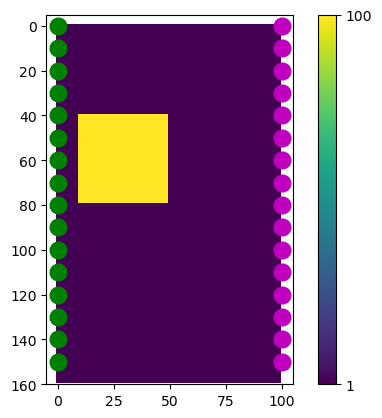
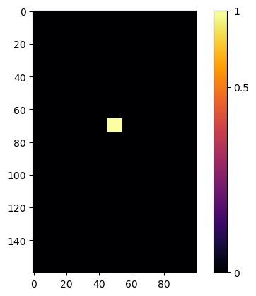
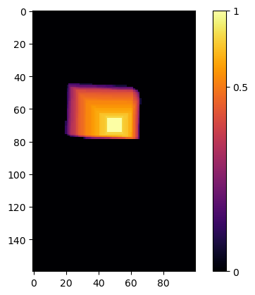
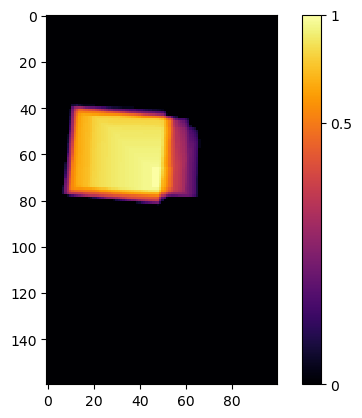
To illustrate the process of HMC sampling, we create a simple experiment where the ground truth velocity model has a high velocity square region. In this experiment, $16\times 16$ transmitter-receiver pairs are placed on the left and right boundary with equal distance $10$ m. Transmitter and receiver locations are represented by green and red dots, respectively. The synthetic traveltime data is generated by FMM method with no noise added. For reconstruction, we choose the number of object in the model equal to $1$, and show the progress of HMC sampling in Fig. 5. From the result, we can see the first $20$ samples are still very close to the initial model. With $100$ samples, HMC sampling starts to move towards the ground truth (high probability region). And with $500$ samples, the HMC sampled probability map is very close to our expectation.

(a)

(b)

(c)

(d)

Figure 5: Results of testing example (a) Ground truth velocity model (b) Probability map with $20$ samples (c) Probability map with $100$ samples (d) Probability map with $500$ samples.

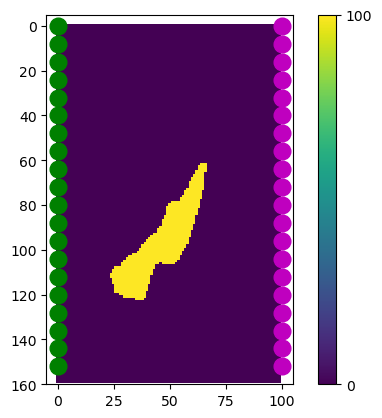
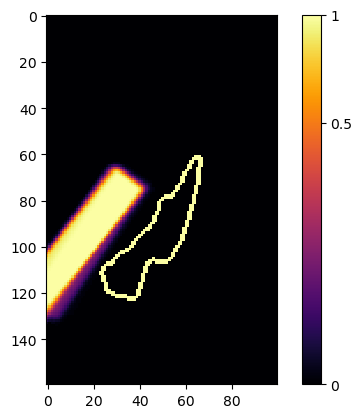
For the next experiment, we use a slightly more complicated ground truth model. In this experiment, $20\times 20$ transmitter-receiver pairs are placed on the left and right boundary and these transceivers are placed with equal distance $8$ m. We show the ground truth model, with the locations of transmitter as green dots and receivers as red dots in Fig. 6 (a). The synthetic traveltime data is generated by FMM method, and we run our experiments on both noiseless and noisy measures. The noisy measurements are generated by adding independent Gaussian noise into each measurements. That means each measurement is $\tilde{t_{i}}=t_{i}+\epsilon_{i}$, where $t_{i}$ is the traveltime from FMM and $\epsilon_{i}$ is the added noise. The added noise is zero mean and independent of each measurement, thus $E(\epsilon_{i})=0$ and $E(\epsilon_{i}\epsilon_{j})=0$. The signal-to-noise (SNR) is set to be $10$db, thus the covariance matrix of the measurements is a diagonal matrix with $E(\epsilon_{i}^{2})=t_{i}^{2}/10$.

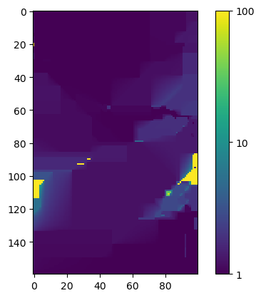
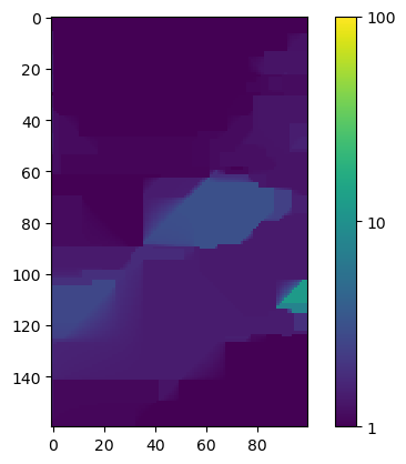
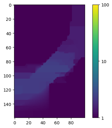
For comparison, we use the bent ray reconstruction with simultaneous iterative reconstruction technique (SIRT), where the models are calculated on a regular grid with $100\times 160$ cells. In SIRT, we use the $L_{1}$ norm of total variation as regularization, where the cost function is a combination of data fitting and weighted regularization term. To make the best possible results, we put additional constraints on the value of reconstructed velocity, $1\leq v\leq 100$ m/s and try different regularization weights. Fig. 6 (b) shows the reconstructed velocity model using noiseless data, with regularization weight equal to $0.05$. The result is very far from the ground truth - it has a few high velocity cells close to the transmitters and receivers. This behavior fits our expectation because the cells close to the transceivers are most sensitive to the change of traveltime. In Fig. 6 (c)(d) we show the results by increasing the regularization weight to $0.1$ and $0.2$. When we increase the weight of regularization, it favors the result with piece-wise constant velocity model. Although in Fig. 6 (d) it successfully identifies that the high velocity region is roughly within a $45^{\circ}$ angle, but it provides very poor result for the exact location.

(a)

(b)

(c)

(d)

Figure 6: Results from SIRT (a) Ground truth model (b) Reconstructed velocity model with regularization weight $\alpha=0.05$ (c) Result with $\alpha=0.1$ (d) Result with $\alpha=0.2$

(a)

(b)

(c)

(d)

Figure 7: Results from HMC sampling with $5000$ samples (a) One object, noiseless (b) One object, SNR = $10$dB (c) Three objects, noiseless (d) Three objects, SNR = $10$dB

(a)

(b)

(c)

(d)

(e)

(f)

(g)

(h)

Figure 8: Results from HMC sampling when estimating one object model with (a) $100$ samples (b) $500$ samples (c) $1000$ samples (d) $5000$ samples, and three objects with (e) $100$ samples (f) $500$ samples (g) $1000$ samples (h) $5000$ samples

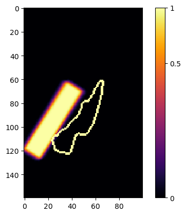
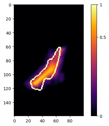
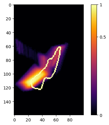
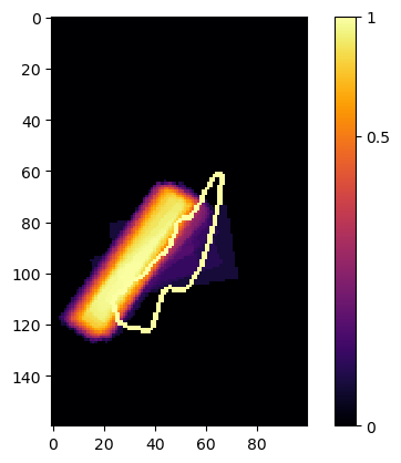
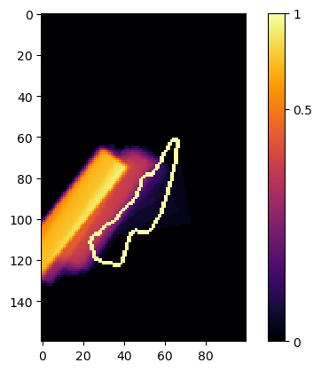
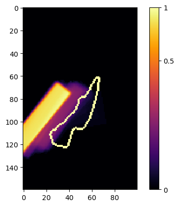
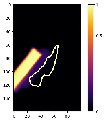
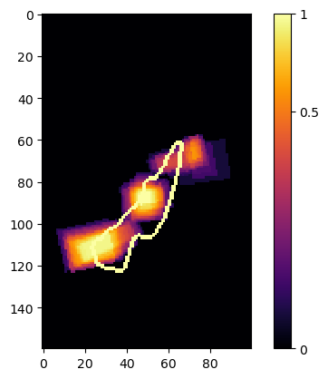
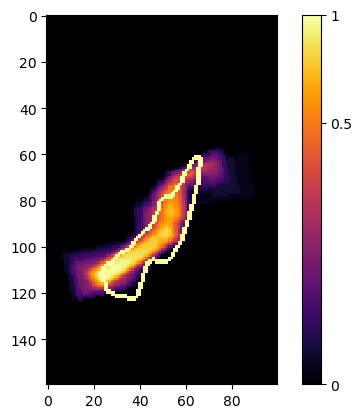
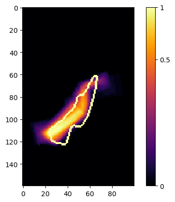
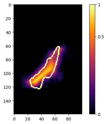
We show the ”probability map” from our approach in Fig 7. In this experiment, we take $5000$ samples and drop the first $1000$ to avoid the transient state of Markov Chain. For better visualization, we mark the boundary of ground truth model. Fig 7 (a)(b) shows that one object model can recover the approximate location and angle of high velocity region, but also has limited ability to model the shape. However we still observe some level of mismatch, especially for the shift in the horizontal axis. This effect is very common in traveltime tomography. In our setting, most transmitter-receiver pairs have stronger horizontal component. Thus, we expect to have better resolution along the vertical axis as compared to the horizontal axis.

Fig. 7 (c)(d) shows the result for the three object model. Obviously, the three object model provides much better approximation for the shape, but it is also more sensitive to noise. The reason is that three object model has more degrees of freedom, thus it could ‘over-fit‘ the data. Also, we want to mention that when running HMC with limited samples a more complex model may not provide better results. The reason is that if a model has more degree of freedom, it also requires many more samples to converge to the target probability distribution. With limited samples, the Markov Chain may stay in transient states and thus the sampled probability will not reflect the target distribution. We show the results for different number of samples in Fig. 8, which shows that one object model requires fewer samples to converge. For more detail on this topic, please refer to [22].

Note that Fig. 8 (a-d) shows that the result converges to a wrong location (horizontal shift from ground truth). Because most transmitter-receiver pairs have a stronger horizontal component, we expect to have better resolution along the vertical axis as compared to the horizontal axis. That means that two models where their objects shifted with respect to each other along the horizontal direction could have very similar probability. Fig. 8 (a) may give the impression that the result with few samples is better, but it is actually still in a transient period of Markov Chain moving from the initial state.

Compared to the result in Fig. 6, it is obvious that our approach provides a more accurate reconstructed model for the high velocity structure in the sparse measurements case. The result from SIRT suffers from the “curse of dimensionality”, that is, we only have $20\times 20$ data points but we try to recover $100\times 160$ unknown variables. Although we use total variation as the regularization (which favors a piece-wise constant solution), no matter how we change the weight of regularization, SIRT still fails to provide a good estimate of the location of high velocity zones. The reason is that the data is “too sparse” for SIRT. For estimating the velocity in a cell, we need at least two trajectory passing through it. However, in this experiment the ratio between the number of cells and trajectories is $2.5\%$ and most cells have zero or one trajectory through them. Thus, SIRT can assign the high velocity cells arbitrary along the trajectory and it usually estimates the high velocity structure to be closed to the transceivers, which is a common phantom for SIRT with sparse measurements. The reason is that the velocity in these areas is most sensitive to the change of cost function. Thus, SIRT will favor a velocity model that changes most near the transmitters or receivers, while our approach is more robust when only limited amounts of data are available.

VI Conclusion

The main purpose of this paper is to propose a new approach for the reconstruction of velocity models in travel time tomography. We use the object-based model to approximate the velocity structure, and formulate the reconstruction as a probability sampling problem in parameter space. We use the misfit of traveltime to define a potential function, and apply HMC to sample the parameter space. Typically HMC is considered to be too computationally expensive for tomography problems, but we demonstrate that by using some specific type of fundamental objects for high contrast media, the traveltime calculation can be greatly simplified. Compared to the conventional fast marching method on the cell, our approach provides similar results with much less computations. This algorithm makes HMC sampling computationally feasible.

In simulations, our approach successfully finds possible models and assigns them appearance probability. Especially for limited amounts of data, we show that our algorithm provides significantly better results than typical iterative ray-based reconstruction on cells. The only problem is that even with our fast traveltime calculation, a $20\times 20$ TX-RX, three object model simulation takes about $10$ hours to generate $5000$ samples in a Xeon workstation, which has a $8$ cores INTEL E5-2670 CPU. While SIRT with $L_{1}$ regularization only takes few minutes of computational time, our approach is much more computationally expensive. However, in our algorithm the calculation of cost function is parallalizable and fits into the MapReduce framework. Ideally, the simulation time could be reduced to $1/N$ if we have $N$ machines. With the progress of cloud platform and parallel programming, we believe computation cost would not be a big problem in the future and our approach might be widely accepted.

Future work will be to extend our approach to general cases. For example, the object model can be used not only for high contrast cases but also for general velocity model. Unfortunately, fast traveltime calculations may not be available for general cases. Of course, we can always map the object model into cells and use fast marching method on it but the computational overhead makes the HMC sampling less attractive. We plan to explore the problem of how to define an object model that has an efficient representation of velocity structure, and is also applicable to fast traveltime calculation.

Another topic we would like to explore is that of finding the optimum number of objects in the model. In the early development of our algorithm, we did consider to put the number of objects as a parameter in our model. Then we realize that increasing the number of objects will provide the ability to achieve lower cost function. Thus, without any prior information about the number of objects, in HMC sampling the number of objects will keep growing and the Markov chain sampling never converges. Furthermore, if the number of object grows it implies the number of parameters also grows. At this point, it is still unclear how to change the step size and number of steps dynamically when the dimension changes. We note that recent advances in transdimensional tomography [7] may be useful to quantify the trade-off between the number of objects and computational complexity of our approach. Finally, we mention that the Python implementation of our algorithm is publicly available at https://github.com/STAC-USC.

References

- [1] Agarwal, P., Suri, S.: Surface approximation and geometric partitions. SIAM Journal on Computing 27(4), 1016–1035 (1998)
- [2] Bai, C., Greenhalgh, S.: 3-d non-linear travel-time tomography: Imaging high contrast velocity anomalies. Pure and Applied Geophysics 162(11), 2029–2049 (2005)
- [3] Berryman, J.: Fermat’s principle and nonlinear traveltime tomography. Physical review letters 62(25), 2953–2956 (1989)
- [4] Berryman, J.: Lecture notes on nonlinear inversion and tomography: 1, borehole seismic tomography. Tech. rep., Lawrence Livermore National Lab., CA (United States) (1991)
- [5] Berryman, J.G.: Lecture notes on nonlinear inversion and tomography. Tech. rep. (1991)
- [6] Beydoun, W.B., Keho, T.H.: The paraxial ray method. Geophysics 52(12), 1639–1653 (1987)
- [7] Bodin, T., Sambridge, M., Rawlinson, N., Arroucau, P.: Transdimensional tomography with unknown data noise. Geophysical Journal International 189(3), 1536–1556 (2012)
- [8] Courant, R., Hilbert, D.: Methods of mathematical physics, vol. 1. CUP Archive (1962)
- [9] Engl, H., Hanke, M., Neubauer, A.: Regularization of inverse problems. Springer Netherlands (1996)
- [10] Hastings, W.K.: Monte Carlo sampling methods using markov chains and their applications. Biometrika 57(1), 97–109 (1970)
- [11] Kroon, D.: Accurate fast marching. Toolbox, Matlab Central website 23 (2009)
- [12] Lane Jr, J., Day-Lewis, F., Versteeg, R., Casey, C.: Object-based inversion of crosswell radar tomography data to monitor vegetable oil injection experiments. Journal of Environmental and Engineering Geophysics 9, 63 (2004)
- [13] Lin, Y., Ortega, A.: Reconstruction algorithm for high contrast velocity travel time tomography. In: Acoustics Speech and Signal Processing (ICASSP), 2010 IEEE International Conference on, pp. 1214–1217. IEEE (2010)
- [14] Lin, Y., Ortega, A., Nejad, A., Ershaghi, I.: Waterflood tomography: mapping high contrast permeability structures using injection/production data. In: SPE Western Regional Meeting (2010)
- [15] Lin, Y., Ortega, A., Tafti, T., Ershaghi, I.: Detecting shale discontinuity between different layers using waterflood tomography. In: SPE Western Regional Meeting (2012)
- [16] MacKay, D.J.: Information theory, inference and learning algorithms. Cambridge university press (2003)
- [17] Munk, W., Wunsch, C.: Ocean acoustic tomography: A scheme for large scale monitoring. Deep Sea Research Part A. Oceanographic Research Papers 26(2), 123–161 (1979)
- [18] National Research Council (US). Committee on Fracture Characterization and Fluid Flow: Rock fractures and fluid flow: contemporary understanding and applications. National Academy Press (1996)
- [19] Neal, R.: MCMC using hamiltonian dynamics. Handbook of Markov Chain Monte Carlo 54, 113–162 (2010)
- [20] Ng, A.: Preventing overfitting of cross-validation data. In: Proceedings of the Fourteenth International Conference on Machine Learning, pp. 245–253. Morgan Kaufmann Publishers Inc. (1997)
- [21] Pratt, R.: Seismic waveform inversion in the frequency domain. I. Theory and verification in a physical scale model. Geophysics 64, 888–901 (1999)
- [22] Raftery, A.E., Lewis, S.M.: Implementing mcmc. Markov chain Monte Carlo in practice pp. 115–130 (1996)
- [23] Rawlinson, N., Hauser, J., Sambridge, M.: Seismic ray tracing and wavefront tracking in laterally heterogeneous media. Advances in Geophysics 49, 203–273 (2008)
- [24] Sethian, J.: A fast marching level set method for monotonically advancing fronts. Proceedings of the National Academy of Sciences of the United States of America 93(4), 1591 (1996)
- [25] Sethian, J.A., Popovici, A.M.: 3-d traveltime computation using the fast marching method. Geophysics 64(2), 516–523 (1999)
- [26] Tarantola, A.: Inverse problem theory: Methods for data fitting and model parameter estimation (1987)
- [27] Van Gunsteren, W., Berendsen, H.: A leap-frog algorithm for stochastic dynamics. Molecular Simulation 1(3), 173–185 (1988)
- [28] Vasco, D., Datta-Gupta, A.: Integrating field production history in stochastic reservoir characterization. SPE Formation Evaluation 12(3), 149–156 (1997)
- [29] Vidale, J.E.: Finite-difference calculation of traveltimes in three dimensions. Geophysics 55(5), 521–526 (1990)
- [30] Welge, H.: A simplified method for computing oil recovery by gas or water drive. Petroleum Transactions AIME 195, 91–98 (1952)
- [31] Wilson, D., Ziemann, A., Ostashev, V., Voronovich, A.: An overview of acoustic travel-time tomography in the atmosphere and its potential applications. Acta Acustica united with Acustica 87(6), 721–730 (2001)
- [32] Yeh, T.C.J., Liu, S.: Hydraulic tomography: Development of a new aquifer test method. Water Resources Research 36(8), 2095–2105 (2000)
- [33] Zheglova, P., Farquharson, C.G.: Level set method in seismic inversion: 2D reconstruction of boundaries. Journal of Computational Physics 79, 1249 (2012)