Uniform asymptotic approximation of diffusion to a small target

Abstract

The problem of the time required for a diffusing molecule, within a large bounded domain, to first locate a small target is prevalent in biological modeling. Here we study this problem for a small spherical target. We develop uniform in time asymptotic expansions in the target radius of the solution to the corresponding diffusion equation. Our approach is based on combining expansions of a long-time approximation of the solution, involving the first eigenvalue and eigenfunction of the Laplacian, with expansions of a short-time correction calculated by pseudopotential approximation. These expansions allow the calculation of corresponding expansions of the first passage time density for the diffusing molecule to find the target. We demonstrate the accuracy of our method in approximating the first passage time density and related statistics for the spherically symmetric problem where the domain is a large concentric sphere about a small target centered at the origin.

I Introduction

Diffusion of a molecule to a spherical trap is a classical problem important in chemical kinetics. In an unbounded domain, the problem reduces to the Smoluchowski theory of reaction kinetics. In the context of biological processes, intracellular transport of biomolecules and chemical reactions occur within closed domains with complex geometries Bressloff and Newby (2013). As a first passage time problem, this is closely related to the narrow escape problem, where a diffusing molecule escapes a closed domain through a small opening on the boundary, and the long time behavior has been studied using matched asymptotics Ward and Keller (1993); Condamin et al. (2007); Schuss et al. (2007); Coombs et al. (2009); Pillay et al. (2010); Cheviakov et al. (2010); Chevalier et al. (2011). There are many examples of this type of first passage time problem in biological modeling, including transport of receptors on the plasma membrane of a dendrite Holcman and Schuss (2004); Bressloff et al. (2007), intracellular virus trafficking Lagache and Holcman (2007), molecular motor transport Bressloff and Newby (2011), binding of a transcription factor to a segment of DNA within a nucleus Isaacson et al. (2011), and export of newly transcribed mRNA through nuclear pores Cullen (2003).

Consider a bounded domain $\Omega\subset\mathbb{R}^{3}$, containing a small, absorbing spherical trap, $\Omega_{\epsilon}\subset\Omega$, with radius $\epsilon$ centered at $\bm{r}_{\rm{b}}\in\Omega$. We denote by $\partial\Omega$ the exterior boundary surface to $\Omega$, and by $\partial\Omega_{\epsilon}$ the exterior boundary to $\Omega_{\epsilon}$. The non-trap portion of $\Omega$ is denoted by $\Omega_{\text{free}}=\Omega\setminus\{\Omega_{\epsilon}\cup\partial\Omega_{\epsilon}\}$. Consider a molecule undergoing Brownian motion within $\Omega_{\text{free}}$. We denote by $p(\bm{r},t)$ the probability density that the molecule is at position $\bm{r}\in\Omega_{\text{free}}$ at time $t$ and has not yet encountered the trap. For $D$ the diffusion constant of the molecule, $p(\bm{r},t)$ satisfies the diffusion equation

$$\frac{\partial p}{\partial t}=D\nabla^{2}p(\bm{r},t) ,\quad\bm{r}\in\Omega_{\text{free}},t>0,$$ (1.1a)

$$\partial_{\bm{\eta}}p(\bm{r},t)=0 ,\quad\bm{r}\in\partial\Omega,t>0,$$ (1.1b)

$$p(\bm{r},t)=0 ,\quad\bm{r}\in\partial\Omega_{\epsilon},t>0,$$ (1.1c)

$$p(\bm{r},0)=\delta(\bm{r}-\bm{r}_{0}) ,\quad\bm{r}\in\Omega_{\text{free}},\bm{r}_{0}\in\Omega_{\text{free}}$$ (1.1d)

where $\partial_{\bm{\eta}}$ denotes the partial derivative in the outward normal direction, $\bm{\eta}$, to the boundary. Let $T$ label the random variable for the time at which the molecule first reaches $\partial\Omega_{\epsilon}$. The first passage time cumulative distribution is defined as

$$\mathcal{F}(t)\equiv\operatorname{Prob}[T<t]=1-\int_{\Omega}p(\bm{r},t)d\bm{r}.$$ (1.2)

The solution to (1.1) can be written in terms of an eigenfunction expansion with

$$p(\bm{r},t)=\sum_{n=0}^{\infty}\psi_{n}(\bm{r}_{0})\psi_{n}(\bm{r})e^{-\lambda_{n}t},$$ (1.3)

where the eigenfunctions and eigenvalues satisfy

$$-D\nabla^{2}\psi_{n}(\bm{r})=\lambda_{n}\psi_{n} ,\quad\bm{r}\in\Omega_{\text{free}},$$ (1.4a)

$$\partial_{\bm{\eta}}\psi_{n}=0 ,\quad\bm{r}\in\partial\Omega,$$ (1.4b)

$$\psi_{n}(\bm{r})=0 ,\quad\bm{r}\in\partial\Omega_{\epsilon},$$ (1.4c)

and the eigenfunctions are orthonormal in $L^{2}(\Omega_{\text{free}})$. We order the eigenvalues so that $0<\lambda_{0}\leq\lambda_{1}\leq\dots$. In the limit that the radius of the trap vanishes, the smallest eigenvalue, subsequently called the principal eigenvalue, also vanishes (i.e., $\lambda_{0}\to 0$). Similarly, the corresponding eigenfunction, subsequently called the principal eigenfunction, approaches $\psi_{0}(\bm{r})\to\frac{1}{\sqrt{\left|\Omega\right|}}$ as $\epsilon\to 0$. Corresponding to these limits, the first passage time $T\to\infty$ and $\lim_{t\to\infty}\int_{\Omega_{\text{free}}}p(\bm{r},t)d\bm{r}=1$ as $\epsilon\to 0$. In what follows we let $\operatorname{diam}S$ and $\left|S\right|$ denote the diameter and volume of the set $S\subset\mathbb{R}^{3}$. For $0<\epsilon\ll\operatorname{diam}\Omega$ the asymptotics of the principal eigenvalue are known, and given by $\lambda_{0}\sim\frac{4\pi D}{\left|\Omega\right|}\epsilon$ Ward and Keller (1993) (see also Cheviakov and Ward (2011)). Note that to first order in $\epsilon$, $\lambda_{0}$ depends only on the volume of $\Omega$ and not the domain geometry. Higher order terms which depend on other properties of the domain are discussed in the next section.

The small $\epsilon$ asymptotics of $\lambda_{0}$ motivate a large-time approximation of $p(\bm{r},t)$, based on a separation of time scales. Truncating the eigenfunction expansion (1.3) after the first term gives the long time approximation,

$$p(\bm{r},t)\sim\frac{1}{\left|\Omega\right|}e^{-\frac{4\pi D}{\left|\Omega\right|}\epsilon t},\quad\lambda_{1}t\gg 1,\quad\epsilon\ll\operatorname{diam}\Omega.$$ (1.5)

Note, however, that the initial condition (1.1d) is not satisfied by this expansion. Instead, the initial condition is modified so that the molecule starts from a uniformly distributed initial position with

$$p(\bm{r},0)=\frac{1}{\left|\Omega\right|}.$$ (1.6)

In other words, the long time behavior depends very little on the initial position of the molecule because it is likely to explore a large portion of the domain before locating the trap. The first passage time density is $f(t)\equiv\frac{d}{dt}\mathcal{F}(t)$, where $\mathcal{F}(t)$ is given by (1.2). The long-time, $\lambda_{1}t\gg 1$, approximation of the first passage time density is then

$$f(t)\sim\lambda_{0}e^{-\lambda_{0}t} ,\quad\text{for }\lambda_{1}t\gg 1,$$ (1.7a)

$$\sim\frac{4\pi D\epsilon}{\left|\Omega\right|}e^{-\frac{4\pi D}{\left|\Omega\right|}\epsilon t} ,\quad\text{for }\epsilon\ll\operatorname{diam}\Omega.$$ (1.7b)

The first passage time is therefore approximately an exponential random variable, with mean

$$E[T]\sim\frac{1}{\lambda_{0}} ,\quad\text{for }\lambda_{1}t\gg 1,$$ (1.8a)

$$\sim\frac{\left|\Omega\right|}{4\pi D\epsilon} ,\quad\text{for }\epsilon\ll\operatorname{diam}\Omega.$$ (1.8b)

An exponentially-distributed first passage time is an important assumption in course-grained models, such as the reaction-diffusion master equation (RDME) Gardiner (1996); Van Kampen (2001); Gardiner et al. (1976). (The RDME is a lattice stochastic reaction diffusion model which assumes that reacting chemicals are well mixed within a computational voxel.) More broadly, exponential waiting times are essential for jump processes to be Markovian.

The above long-time approximation motivates several questions. First, when is the non-exponential, short-time behavior of the first passage time important? Second, how does changing the initial position of the molecule effect the approximation? It follows from (1.8a) that the mean binding time is approximately independent of the initial position. On the other hand, as we show here the most likely binding time, called the mode, depends strongly on the initial position. Recently, the importance of the initial position in first passage times in confined domains has been studied in the context of chemical reactions Bénichou et al. (2010), and shown to play a role in quantifying the difference between two or more identically distributed first passage times Mejía-Monasterio et al. (2011); Mattos et al. (2012). More generally, to estimate spatial statistics for the position of the diffusing molecule it is necessary to obtain expansions of not just the first passage time density, $f(t)$, but also the solution to the diffusion equation, $p(\bm{r},t)$.

The first passage time problem in a confined domain has also been studied from the perspective of a continuous time random walk (CTRW) on a finite graph of size $N$ Meyer et al. (2011). Meyer and coworkers obtain exact results for the Laplace transform, which is the moment generating function for the first passage time distribution, and expand the moments for large $N$. They then reconstruct the large $N$ expansion of the first passage time distribution from the moments. These results can also be interpreted as an approximation of the first passage time distribution in the large volume limit. This perspective is closely related to the one considered here; instead of an expansion in large volume, we assume the domain volume is $O(1)$ and expand in terms of the small radius of the target.

Motivated by these and other examples, we develop a uniform in time asymptotic approximation as $\epsilon\to 0$ of the probability density, $p(\bm{r},t)$ (see (2.42)), and the first passage time density, $f(t)$ (see (2.49)), that accounts for non-exponential, small time behavior and the initial position of the molecule. The paper is organized as follows. In Section II we further develop the long time approximation and present the complimentary short time correction based on a pseudopotential approximation. Adding these two estimates we derive a uniform in time asymptotic expansion of $p(\bm{r},t)$ for small $\epsilon$. It must be emphasized that what we call the “short time” correction is not an asymptotic expansion of $p(\bm{r},t)$ as $t\to 0$, but instead is a correction that when added to the long time expansion for any fixed $t$ and $\bm{r}$ gives an asymptotic expansion of $p(\bm{r},t)$ in $\epsilon$. In Section II.3 we use the results of Section II to derive a small $\epsilon$ expansion of the first passage time density (through terms of order $O(\epsilon^{2})$). Finally, in Section III these approximations are compared to the exact solution, exact first passage time density, and several other statistics for a spherical trap concentric to a spherical domain.

II Uniform asymptotic approximation

Our basic approach is to first split $p(\bm{r},t)$ into two components: a large time approximation that will accurately describe the behavior of $p(\bm{r},t)$ for $\lambda_{1}t\gg 1$, and a short time correction to this approximation when $\lambda_{1}t\not\gg 1$. Note, both are defined for all times, but the latter approaches zero as $t\to\infty$, and so only provides a significant contribution for $\lambda_{1}t\not\gg 1$. It should be stressed that the short time correction is not an asymptotic approximation of $p(\bm{r},t)$ as $t\to 0$, but instead serves as a correction to the long time expansion for $\lambda_{1}t\not\gg 1$. We write $p(\bm{r},t)$ as

$$p(\bm{r},t)=p_{\text{\tiny{LT}}}(\bm{r},t)+p_{\text{\tiny{ST}}}(\bm{r},t),$$ (2.1)

where $p_{\text{\tiny{LT}}}$ is the large time approximation and $p_{\text{\tiny{ST}}}$ is the short time correction. We will take $p_{\text{\tiny{LT}}}=\psi_{0}(\bm{r})\psi_{0}(\bm{r}_{0})\exp\left[-\lambda_{0}t\right]$ to be the long time approximation of the eigenfunction expansion (1.3) of $p(\bm{r},t)$. With this choice, $p_{\text{\tiny{LT}}}$ and $p_{\text{\tiny{ST}}}$ satisfy the projected initial conditions

$$p_{\text{\tiny{LT}}}(\bm{r},0) =\left\langle\psi(\bm{r}),\delta(\bm{r}-\bm{r}_{0})\right\rangle\psi(\bm{r})=\psi(\bm{r})\psi(\bm{r}_{0}),$$ (2.2)

$$p_{\text{\tiny{ST}}}(\bm{r},0) =\delta(\bm{r}-\bm{r}_{0})-\psi(\bm{r})\psi(\bm{r}_{0}).$$ (2.3)

Here we have dropped the subscript and subsequently identify $\psi$ and $\lambda$ as the principal eigenfunction and eigenvalue respectively. Using (2.2) and (2.3) as initial conditions, and setting $t=0$ in (2.1), then gives $p(\bm{r},t)=\delta(\bm{r}-\bm{r}_{0})$ as required.

In the next two sections we derive asymptotic expansions of $p_{\text{\tiny{LT}}}$ and $p_{\text{\tiny{ST}}}$ for $\epsilon\ll\operatorname{diam}\Omega$. The expansion of $p_{\text{\tiny{LT}}}$ is based off the principal eigenvalue and eigenfunction expansions developed in Cheviakov and Ward (2011). The expansion of $p_{\text{\tiny{ST}}}$ adapts the pseudopotential method we first used in Isaacson and Isaacson (2009), where uniform in time expansions of $p(\bm{r},t)$ and the first passage time cumulative distribution, $\operatorname{Prob}\left[T<t\right]$, were obtained for $\Omega=\mathbb{R}^{3}$ and $\bm{r}_{\rm{b}}$ the origin. We have found that a direct pseudopotential approximation of (1.1) in bounded domains with Neumann boundary conditions breaks down for large, but finite times. For example, the direct pseudopotential based expansion of $\operatorname{Prob}\left[T<t\right]$ can become negative for large times. This inaccuracy in the pseudopotential approximation arises from the non-zero steady state solution to the limiting $\epsilon=0$ equation. As we see in Section II.2, by projecting out the principal eigenfunction this problem is removed when expanding $p_{\text{\tiny{ST}}}$. This motivated our use of the splitting $p=p_{\text{\tiny{LT}}}+p_{\text{\tiny{ST}}}$.

II.1 Large time asymptotic expansion

Since the initial condition (2.2) is an eigenfunction of the Laplacian, the long time density is given by

$$p_{\text{\tiny{LT}}}(\bm{r},t)=\psi(r)\psi(r_{0})e^{-\lambda t}.$$

As discussed in the Introduction, there are well known asymptotic approximations for small $\epsilon$ of $\psi(r)$ and $\lambda$. These then determine the small $\epsilon$ behavior of $p_{\text{\tiny{LT}}}(\bm{r},t)$. The expansions of $\psi(r)$ and $\lambda$ are typically given in terms of the corresponding no-trap problem where $\epsilon=0$. Let $G(\bm{r},\bm{r}^{\prime},t)$ denote the fundamental solution to the diffusion equation in $\Omega$ (i.e. the $\epsilon=0$ problem), then

$$\frac{\partial}{\partial t}G(\bm{r},\bm{r}^{\prime},t) =D\nabla^{2}G(\bm{r},\bm{r}^{\prime},t),\quad\bm{r}\in\Omega,$$ (2.4)

$$G(\bm{r},\bm{r}^{\prime},0) =\delta(\bm{r}-\bm{r}^{\prime}),\quad\bm{r}\in\Omega,$$

with the no-flux Neumann boundary condition

$$\partial_{\bm{\eta}}G(\bm{r},\bm{r}^{\prime},t)=0,\quad\bm{r}\in\partial\Omega.$$ (2.5)

We will also need the corresponding solution to the time-independent problem, the pseudo-Green’s function $U(\bm{r},\bm{r}^{\prime})$, satisfying

$$D\nabla^{2}U(\bm{r},\bm{r}^{\prime})=\frac{1}{\left|\Omega\right|}-\delta(\bm{r}-\bm{r}^{\prime}),\quad\bm{r}\in\Omega,$$ (2.6)

with the no-flux Neumann boundary condition

$$\partial_{\bm{\eta}}U(\bm{r},\bm{r}^{\prime})=0,\quad\bm{r}\in\partial\Omega,$$ (2.7)

and the normalization condition

$$\int_{\Omega}U(\bm{r},\bm{r}^{\prime})d\bm{r}=0.$$ (2.8)

Within the derivative terms in (2.4) we can replace $G(\bm{r},\bm{r}^{\prime},t)$ by $G(\bm{r},\bm{r}^{\prime},t)-\left|\Omega\right|^{-1}$. Integrating the resulting equation in $t$ on $(0,\infty)$, and using the uniqueness of the solution to (2.6) with the boundary condition (2.7) and the normalization (2.8), we find

$$\int_{0}^{\infty}\left(G(\bm{r},\bm{r}^{\prime},t)-\frac{1}{\left|\Omega\right|}\right)dt=U(\bm{r},\bm{r}^{\prime}).$$ (2.9)

Here the term $\left|\Omega\right|^{-1}$ is necessary to guarantee convergence of the integral. Finally, we denote by $\gamma$ the value of the regular part of $U(\bm{r},\bm{r}_{\rm{b}})$ at $\bm{r}=\bm{r}_{\rm{b}}$,

$$\gamma\equiv\lim_{\bm{r}\to\bm{r}_{\rm{b}}}\left[U(\bm{r},\bm{r}_{\rm{b}})-\frac{1}{4\pi D\left|\bm{r}-\bm{r}_{\rm{b}}\right|}\right].$$ (2.10)

Let $\hat{k}=4\pi D$. As derived in Cheviakov and Ward (2011), the asymptotic expansions of the principal eigenvalue and eigenfunction for small $\epsilon$ are

$$\lambda\sim\lambda_{\text{\tiny{LT}}}\equiv\frac{\hat{k}}{\left|\Omega\right|}\left(1-\hat{k}\gamma\epsilon\right)\epsilon,$$ (2.11)

and

$$\psi(\bm{r}) \sim\frac{1}{\sqrt{\left|\Omega\right|}}+\epsilon\psi^{(1)}(\bm{r})+\epsilon^{2}\psi^{(2)}(\bm{r})$$

$$\begin{aligned} =\frac{1}{\sqrt{\left|\Omega\right|}}&\Bigg{[}1-\epsilon\hat{k}U(\bm{r},\bm{r}_{\rm{b}})-\epsilon^{2}\hat{k}^{2}\Bigg{(}-\gamma U(\bm{r},\bm{r}_{\rm{b}})\\ &+\frac{1}{\left|\Omega\right|}\int_{\Omega}U(\bm{r},\bm{r}^{\prime})U(\bm{r}^{\prime},\bm{r}_{\rm{b}})d\bm{r}^{\prime}\Bigg{)}\Bigg{]}+\epsilon^{2}\bar{\Psi}.\end{aligned}$$ (2.12)

Here $\bar{\Psi}$ denotes the spatial average of the second order term and is given by Cheviakov and Ward (2011)

$$\bar{\Psi}=-\frac{\hat{k}^{2}}{2\left|\Omega\right|^{\frac{3}{2}}}\int_{\Omega}\left(U(\bm{r},\bm{r}_{\rm{b}})\right)^{2}d\bm{r}.$$ (2.13)

Note, the second order term in (2.12) is not explicitly derived in Cheviakov and Ward (2011), but can be found by solving equation (2.20) (of Cheviakov and Ward (2011)) with the normalization (2.13). The corresponding expansion of the initial condition, $p_{\text{\tiny{LT}}}(\bm{r},0)$, in $\epsilon$ is

$$p_{\text{\tiny{LT}}}(\bm{r},0)\sim\frac{1}{\left|\Omega\right|}+w^{(1)}(\bm{r},\bm{r}_{0})\epsilon+w^{(2)}(\bm{r},\bm{r}_{0})\epsilon^{2},$$

where the functions $w^{(n)}(\bm{r},\bm{r}_{0})$ are obtained from substituting the asymptotic approximations of the principal eigenfunction and eigenvalue into (2.2) and collecting terms in $\epsilon$. We find that

$$w^{(1)}(\bm{r},\bm{r}_{0})=-\frac{\hat{k}}{\left|\Omega\right|}\Big{(}U(\bm{r},\bm{r}_{\rm{b}})+U(\bm{r}_{0},\bm{r}_{\rm{b}})\Big{)},$$ (2.14)

$$\begin{split}w^{(2)}(\bm{r},\bm{r}_{0})&=\frac{2\bar{\Psi}}{\sqrt{\left|\Omega\right|}}+\frac{\hat{k}^{2}}{\left|\Omega\right|}U(\bm{r},\bm{r}_{\rm{b}})U(\bm{r}_{0},\bm{r}_{\rm{b}})\\ &\quad+\frac{\hat{k}^{2}\gamma}{\left|\Omega\right|}\left[U(\bm{r},\bm{r}_{\rm{b}})+U(\bm{r}_{0},\bm{r}_{\rm{b}})\right]\\ &-\frac{\hat{k}^{2}}{\left|\Omega\right|^{2}}\int_{\Omega}\left[U(\bm{r},\bm{r}^{\prime})+U(\bm{r}_{0},\bm{r}^{\prime})\right]U(\bm{r}^{\prime},\bm{r}_{\rm{b}})d\bm{r}^{\prime},\end{split}$$ (2.15)

so that the small $\epsilon$ expansion of $p_{\text{\tiny{LT}}}(\bm{r},t)$ is then

$$p_{\text{\tiny{LT}}}(\bm{r},t)\sim\left[\frac{1}{\left|\Omega\right|}+w^{(1)}(\bm{r},\bm{r}_{0})\epsilon+w^{(2)}(\bm{r},\bm{r}_{0})\epsilon^{2}\right]e^{-\lambda_{\text{\tiny{LT}}}t}.$$ (2.16)

II.2 Short time correction asymptotic expansion

To construct an asymptotic approximation to $p_{\text{\tiny{ST}}}(\bm{r},t)$ for small $\epsilon$, we replace the trap boundary condition by a sink term in the PDE involving a Fermi pseudopotential operator Fermi (1936); Huang and Yang (1957), subsequently denoted by $V$. The boundary condition $p_{\text{\tiny{ST}}}(\bm{r},t)=0$ for $\bm{r}\in\partial\Omega_{\epsilon}$ is replaced by the sink term

$$-Vp_{\text{\tiny{ST}}}(\bm{r},t)\equiv-\epsilon\hat{k}\frac{\partial}{\partial\left|\bm{r}-\bm{r}_{\rm{b}}\right|}\Big{[}\left|\bm{r}-\bm{r}_{\rm{b}}\right|p_{\text{\tiny{ST}}}(\bm{r},t)\Big{]}_{\bm{r}=\bm{r}_{\rm{b}}}\\ \times\delta(\bm{r}-\bm{r}_{\rm{b}})$$ (2.17)

For $r=\left|\bm{r}\right|$, in the special case that $\bm{r}_{\rm{b}}=\bm{0}$ is the origin, this reduces to

$$-Vp_{\text{\tiny{ST}}}(\bm{r},t)\equiv-\epsilon\hat{k}\frac{\partial}{\partial r}\left[rp_{\text{\tiny{ST}}}(\bm{r},t)\right]_{\bm{r}=\bm{0}}\delta(\bm{r}).$$ (2.18)

Before we proceed with the pseudopotential approximation, it is instructive to consider why for an equivalent problem in 1D, replacing the absorbing boundary condition with a sink term makes the problem easier to solve. To see how this idea breaks down in higher dimensions, and to motivate the pseudopotential operator, we apply the Laplace transform to (1.1a) (with $p$ replaced by $p_{\text{\tiny{ST}}}$ and the initial condition modified to (2.3)). We replace the Dirichlet boundary condition (1.1c) by a delta function absorption term on the right hand side. If $\tilde{p}_{\text{\tiny{ST}}}(\bm{r},s)$ denotes the Laplace transform of $p_{\text{\tiny{ST}}}(\bm{r},t)$, then we find

$$-D\nabla^{2}\tilde{p}_{\text{\tiny{ST}}}+s\tilde{p}_{\text{\tiny{ST}}}=\delta(\bm{r}-\bm{r}_{0})-\psi(\bm{r})\psi(\bm{r}_{0})\\ -C\delta(\bm{r}-\bm{r}_{\rm{b}})\tilde{p}_{\text{\tiny{ST}}},$$ (2.19)

so that absorption by the target occurs when the center of the target is reached (at some rate $C$ that is to be determined). Using the Green’s function of the diffusion equation (2.4), we can write the solution as

$$\tilde{p}_{\text{\tiny{ST}}}(\bm{r},s)=\tilde{G}(\bm{r},\bm{r}_{0},s)-\psi(\bm{r}_{0})\int_{\Omega}\tilde{G}(\bm{r},\bm{r}^{\prime},s)\psi(\bm{r}^{\prime})d\bm{r}^{\prime}\\ -C\tilde{p}_{\text{\tiny{ST}}}(\bm{r}_{\rm{b}},s)\tilde{G}(\bm{r},\bm{r}_{\rm{b}},s).$$ (2.20)

To solve the above equation, we need only take the limit $\bm{r}\to\bm{r}_{\rm{b}}$ and solve for $\tilde{p}_{\text{\tiny{ST}}}(\bm{r}_{\rm{b}},s)$. However, we observe that for dimensions greater than one $\lim_{\bm{r}\to\bm{r}_{\rm{b}}}\tilde{G}(\bm{r},\bm{r}_{\rm{b}},s)=\infty$, which is why the naive approach breaks down. There are a few different methods for adapting this idea to work in higher dimensions, namely matched asymptotics Ward and Keller (1993) and pseudo potential operators, which is the approach that we use here.

The pseudopotential operator, $V$, was developed so that the operator

$$D\nabla^{2}-V$$

on $\Omega$ provides an asymptotic approximation in $\epsilon$ of $D\nabla^{2}$ on $\Omega_{\text{free}}$ with a zero Dirichlet boundary condition on $\partial\Omega_{\epsilon}$ Huang and Yang (1957). It was originally constructed for approximating hard core potentials in quantum mechanical scattering problems Fermi (1936); Huang and Yang (1957), but has also been used in the estimation of diffusion-limited reaction rates in two-dimensional periodic systems Torney and Goldstein (1987). The operator was derived in Huang and Yang (1957) by expanding the eigenfunctions (1.4), $\psi_{n}(\bm{r})$, in a basis of spherical harmonics and then analytically continuing the domain of definition of each eigenfunction into the interior of the sphere, $\Omega_{\epsilon}$. On $\Omega$, it was found that formally

$$D\nabla^{2}\psi_{n}(\bm{r})+\lambda_{n}\psi_{n}(\bm{r})=V\psi_{n}(\bm{r})+O(\epsilon^{3}).$$

When $\Omega=\mathbb{R}^{3}$, it has been shown that the asymptotic expansion for small $\epsilon$ of the solution to the diffusion equation with pseudopotential interaction agrees with the direct asymptotic expansion in $\epsilon$ of the exact solution to the diffusion equation with a zero Dirichlet boundary condition, $p(\bm{r},t)=0$ for $\bm{r}\in\partial\Omega_{\epsilon}$, up through terms of order $O(\epsilon^{2})$ Isaacson and Isaacson (2009).

The pseudopotential approximation for $p_{\text{\tiny{ST}}}(\bm{r},t)$ is that

$$\frac{\partial}{\partial t}p_{\text{\tiny{ST}}}(\bm{r},t)=D\nabla^{2}p_{\text{\tiny{ST}}}(\bm{r},t)-Vp_{\text{\tiny{ST}}}(\bm{r},t)$$ (2.21)

for $\bm{r}\in\Omega$, with the initial condition (2.3) and a no-flux Neumann boundary condition on $\partial\Omega$. In Albeverio et al. (1988, 1995); Albeverio and Kurasov (2000); Dell’Antonio et al. (1998) several approaches are developed for rigorously defining pseudopotential interactions (usually called point interactions or singular perturbations of the Laplacian in those works). Following these works, in particular Dell’Antonio et al. (1998); Isaacson and Isaacson (2009), we split $p_{\text{\tiny{ST}}}(\bm{r},t)$ into a regular part, $\phi(\bm{r},t)$, and a singular part, $q(t)U(\bm{r},\bm{r}_{\rm{b}})$, so that

$$p_{\text{\tiny{ST}}}(\bm{r},t)=\phi(\bm{r},t)+q(t)U(\bm{r},\bm{r}_{\rm{b}}).$$ (2.22)

Here it is assumed that $\phi(\bm{r},t)$ is “nice” as $\bm{r}\to\bm{r}_{\rm{b}}$. In Appendix A we give a more detailed motivation for this representation.

To find the asymptotic expansion of $p_{\text{\tiny{ST}}}(\bm{r},t)$ for small $\epsilon$, we begin by formulating a closed integral equation for $\phi(\bm{r},t)$. As described in Cheviakov and Ward (2011), we can separate $U(\bm{r},\bm{r}_{\rm{b}})$ into a component that is regular at $\bm{r}=\bm{r}_{\rm{b}}$, denoted by $R(\bm{r},\bm{r}_{\rm{b}})$, and a singular part, $\hat{k}^{-1}\left|\bm{r}-\bm{r}_{\rm{b}}\right|^{-1}$, so that

$$U(\bm{r},\bm{r}_{\rm{b}})=R(\bm{r},\bm{r}_{\rm{b}})+\frac{1}{\hat{k}\left|\bm{r}-\bm{r}_{\rm{b}}\right|}.$$

Note that the pseudopotential applied to the singular part of $U(\bm{r},\bm{r}_{\rm{b}})$ is zero. The action of the pseudopotential on the representation (2.22) is therefore

$$V\left[\phi(\bm{r},t)+q(t)U(\bm{r},\bm{r}_{\rm{b}})\right] =\epsilon\hat{k}\left[\phi(\bm{r}_{\rm{b}},t)+\gamma q(t)\right]\delta(\bm{r}-\bm{r}_{\rm{b}}),$$

as $\gamma=R(\bm{r}_{\rm{b}},\bm{r}_{\rm{b}})$ by (2.10). Substituting the representation (2.22) of $p_{\text{\tiny{ST}}}(\bm{r},t)$ into (2.21), we find

$$\frac{\partial\phi}{\partial t}=D\nabla^{2}\phi-\frac{dq}{dt}U(\bm{r},\bm{r}_{\rm{b}})+q(t)\left(\frac{1}{\left|\Omega\right|}-\delta(\bm{r}-\bm{r}_{\rm{b}})\right)\\ -\epsilon\hat{k}\left(\phi(\bm{r}_{\rm{b}},t)+\gamma q(t)\right)\delta(\bm{r}-\bm{r}_{\rm{b}}).$$ (2.23)

We enforce the point boundary condition that the delta function terms should cancel Dell’Antonio et al. (1998); Isaacson and Isaacson (2009) so that

$$q(t)=-\frac{\epsilon\hat{k}}{1+\epsilon\hat{k}\gamma}\phi(\bm{r}_{\rm{b}},t).$$ (2.24)

After substituting (2.24) into (2.22) and rearranging terms we find that

$$p_{\text{\tiny{ST}}}(\bm{r},t)=\left(1-\frac{\epsilon\hat{k}}{1+\epsilon\hat{k}\gamma}U(\bm{r},\bm{r}_{\rm{b}})\right)\phi(\bm{r}_{\rm{b}},t)\\ +(\phi(\bm{r},t)-\phi(\bm{r}_{\rm{b}},t)).$$ (2.25)

If the starting position is close to the target, the last term on the right hand side is expected to be small. It follows that space and time are approximately decoupled, which is consistent with the results of the CTRW approach found in Meyer et al. (2011).

By (2.24), equation (2.23) simplifies to

$$\frac{\partial\phi}{\partial t}=D\nabla^{2}\phi-\frac{dq}{dt}U(\bm{r},\bm{r}_{\rm{b}})+\frac{1}{\left|\Omega\right|}q(t).$$ (2.26)

Using Duhamel’s principle we find that

$$\phi( \bm{r},t)=\int_{\Omega}G(\bm{r},\bm{r}^{\prime},t)\phi(\bm{r}^{\prime},0)d\bm{r}^{\prime}$$

$$-\int_{0}^{t}\int_{\Omega}G(\bm{r},\bm{r}^{\prime},t-s)\left(\frac{dq}{ds}U(\bm{r}^{\prime},\bm{r}_{\rm{b}})-\frac{q(s)}{\left|\Omega\right|}\right)d\bm{r}^{\prime}ds.$$ (2.27)

Integrating by parts we find

$$\int_{0}^{t}G(\bm{r},\bm{r}^{\prime},t-s)\frac{dq}{ds}ds=\int_{0}^{t}D\nabla^{2}G(\bm{r},\bm{r}^{\prime},t-s)q(s)ds\\ +q(t)\delta(\bm{r}-\bm{r}^{\prime})-q(0)G(\bm{r},\bm{r}^{\prime},t),$$ (2.28)

while the no-flux boundary condition implies

$$\int_{\Omega}D\nabla^{2}G(\bm{r},\bm{r}^{\prime},t-s)U(\bm{r}^{\prime},\bm{r}_{\rm{b}})d\bm{r}^{\prime}$$ (2.29)

$$\quad=\int_{\Omega}G(\bm{r},\bm{r}^{\prime},t-s)D\nabla^{2}U(\bm{r}^{\prime},\bm{r}_{\rm{b}})d\bm{r}^{\prime}$$ (2.30)

$$\quad=\int_{\Omega}G(\bm{r},\bm{r}^{\prime},t-s)\left(\frac{1}{\left|\Omega\right|}-\delta(\bm{r}^{\prime}-\bm{r}_{\rm{b}})\right)d\bm{r}^{\prime}$$ (2.31)

$$\quad=\frac{1}{\left|\Omega\right|}-G(\bm{r},\bm{r}_{\rm{b}},t-s).$$ (2.32)

Using the two preceding identities, it follows that (II.2) simplifies to

$$\phi(\bm{r},t) =-q(t)U(\bm{r},\bm{r}_{\rm{b}})+\int_{0}^{t}G(\bm{r},\bm{r}_{\rm{b}},t-s)q(s)ds$$

$$\phantom{-}\quad+\int_{\Omega}G(\bm{r},\bm{r}^{\prime},t)\left[\phi(\bm{r}^{\prime},0)+q(0)U(\bm{r}^{\prime},\bm{r}_{\rm{b}})\right]d\bm{r}^{\prime}.$$ (2.33)

Eliminating $q(t)$ with the point boundary condition (2.24) gives

$$\phi(\bm{r},t)=\int_{\Omega}G(\bm{r},\bm{r}^{\prime},t)p_{\text{\tiny{ST}}}(\bm{r}^{\prime},0)d\bm{r}^{\prime}\\ +\frac{\hat{k}\epsilon}{1+\gamma\hat{k}\epsilon}\bigg{[}U(\bm{r},\bm{r}_{\rm{b}})\phi(\bm{r}_{\rm{b}},t)\\ \left.-\int_{0}^{t}G(\bm{r},\bm{r}_{\rm{b}},t-s)\phi(\bm{r}_{\rm{b}},s)ds\right].$$ (2.34)

We now use the integral equation (2.34) to find an asymptotic expansion of $p_{\text{\tiny{ST}}}(\bm{r},t)$ in $\epsilon$. Let

$$p_{\text{\tiny{ST}}}(\bm{r},t)\sim p_{\text{\tiny{ST}}}^{(0)}(\bm{r},t)+p_{\text{\tiny{ST}}}^{(1)}(\bm{r},t)\epsilon+p_{\text{\tiny{ST}}}^{(2)}(\bm{r},t)\epsilon^{2}.$$

Similarly, we define the expansion of the regular part of $p_{\text{\tiny{ST}}}(\bm{r},t)$ by

$$\phi(\bm{r},t)\sim\phi^{(0)}(\bm{r},t)+\phi^{(1)}(\bm{r},t)\epsilon+\phi^{(2)}(\bm{r},t)\epsilon^{2}.$$

Using (2.24) we identify the expansion terms of $p_{\text{\tiny{ST}}}(\bm{r},t)$ as

$$p_{\text{\tiny{ST}}}^{(0)}(\bm{r},t) =\phi^{(0)}(\bm{r},t),$$

$$p_{\text{\tiny{ST}}}^{(1)}(\bm{r},t) =\phi^{(1)}(\bm{r},t)-\hat{k}\phi^{(0)}(\bm{r}_{\rm{b}},t)U(\bm{r},\bm{r}_{\rm{b}}),$$

$$p_{\text{\tiny{ST}}}^{(2)}(\bm{r},t) =\phi^{(2)}(\bm{r},t)-\hat{k}\left(\phi^{(1)}(\bm{r}_{\rm{b}},t)-\hat{k}\gamma\phi^{(0)}(\bm{r}_{\rm{b}},t)\right)U(\bm{r},\bm{r}_{\rm{b}}).$$

The principal eigenvalue and eigenfunction expansions of the previous section imply that

$$p_{\text{\tiny{ST}}}(\bm{r},0)\sim\delta(\bm{r}-\bm{r}_{0})-\frac{1}{\left|\Omega\right|}-w^{(1)}(\bm{r},\bm{r}_{0})\epsilon-w^{(2)}(\bm{r},\bm{r}_{0})\epsilon^{2}.$$

Substituting this expansion into (2.34) yields

$$\phi^{(0)}(\bm{r},t)=G(\bm{r},\bm{r}_{0},t)-\frac{1}{\left|\Omega\right|},$$ (2.35)

$$\begin{split}\phi^{(1)}(\bm{r},t)&=\hat{k}U(\bm{r},\bm{r}_{\rm{b}})\phi^{(0)}(\bm{r}_{\rm{b}},t)+\frac{\hat{k}}{\left|\Omega\right|}U(\bm{r}_{0},\bm{r}_{\rm{b}})\\ &\quad-\hat{k}\int_{0}^{t}G(\bm{r},\bm{r}_{\rm{b}},t-s)\phi^{(0)}(\bm{r}_{\rm{b}},s)ds\\ &\quad+\frac{\hat{k}}{\left|\Omega\right|}\int_{\Omega}G(\bm{r},\bm{r}^{\prime},t)U(\bm{r}^{\prime},\bm{r}_{\rm{b}})d\bm{r}^{\prime},\end{split}$$ (2.36)

and

$$\phi^{(2)}(\bm{r},t)=-\hat{k}^{2}\gamma U(\bm{r},\bm{r}_{\rm{b}})\phi^{(0)}(\bm{r}_{\rm{b}},t)+\hat{k}U(\bm{r},\bm{r}_{\rm{b}})\phi^{(1)}(\bm{r}_{\rm{b}},t)+\hat{k}^{2}\gamma\int_{0}^{t}G(\bm{r},\bm{r}_{\rm{b}},t-s)\phi^{(0)}(\bm{r}_{\rm{b}},s)ds\\ -\hat{k}\int_{0}^{t}G(\bm{r},\bm{r}_{\rm{b}},t-s)\phi^{(1)}(\bm{r}_{\rm{b}},s)ds-\int_{\Omega}G(\bm{r},\bm{r}^{\prime},t)w^{(2)}(\bm{r}^{\prime},\bm{r}_{0})d\bm{r}^{\prime}.$$ (2.37)

Evaluating (2.37) requires the calculation of $\phi^{(1)}(\bm{r}_{\rm{b}},t)=\lim_{\bm{r}\to\bm{r}_{\rm{b}}}\phi^{(1)}(\bm{r},t)$. Let $G_{0}(\bm{r},\bm{r}^{\prime},t)=G(\bm{r},\bm{r}^{\prime},t)-\frac{1}{\left|\Omega\right|}$. Using (2.9) we have that

$$\begin{split}&U(\bm{r},\bm{r}_{\rm{b}})\phi^{(0)}(\bm{r}_{\rm{b}},t)-\int_{0}^{t}G(\bm{r},\bm{r}_{\rm{b}},t-s)\phi^{(0)}(\bm{r}_{\rm{b}},s)ds\\ &\quad=\int_{0}^{t}\left[\phi^{(0)}(\bm{r}_{\rm{b}},t)-\phi^{(0)}(\bm{r}_{\rm{b}},t-s)\right]G_{0}(\bm{r},\bm{r}_{\rm{b}},s)ds\\ &\quad\qquad+\phi^{(0)}(\bm{r}_{\rm{b}},t)\int_{t}^{\infty}G_{0}(\bm{r},\bm{r}_{\rm{b}},s)ds\\ &\quad\qquad-\frac{1}{\left|\Omega\right|}\int_{0}^{t}\phi^{(0)}(\bm{r}_{\rm{b}},s)ds.\end{split}$$

Combining this expression with the identity

$$\int_{\Omega}G(\bm{r},\bm{r}^{\prime},t)U(\bm{r}^{\prime},\bm{r}_{\rm{b}})d\bm{r}^{\prime}=\int_{t}^{\infty}G_{0}(\bm{r},\bm{r}_{\rm{b}},s)ds,$$

reusing (2.9), and taking the limit $\bm{r}\to\bm{r}_{\rm{b}}$, we find

$$\begin{split}&\phi^{(1)}(\bm{r}_{\rm{b}},t)=\frac{\hat{k}}{\left|\Omega\right|}\int_{t}^{\infty}\phi^{(0)}(\bm{r}_{\rm{b}},s)ds\\ &+\hat{k}G(\bm{r}_{\rm{b}},\bm{r}_{0},t)\int_{t}^{\infty}G_{0}(\bm{r}_{\rm{b}},\bm{r}_{\rm{b}},s)ds\\ &-\hat{k}\int_{0}^{t}\bigg{[}G(\bm{r}_{\rm{b}},\bm{r}_{0},t-s)-G(\bm{r}_{\rm{b}},\bm{r}_{0},t)\bigg{]}G_{0}(\bm{r}_{\rm{b}},\bm{r}_{\rm{b}},s)ds.\end{split}$$ (2.38)

Note, in the first integral $G_{0}(\bm{r}_{\rm{b}},\bm{r}_{\rm{b}},s)$ will scale like $s^{-3/2}$ as $s\to 0$. This singularity is weakened by the $G(\bm{r}_{\rm{b}},\bm{r}_{0},t-s)-G(\bm{r}_{\rm{b}},\bm{r}_{0},t)$ term, which formally scales like $s$ as $s\to 0$ (for fixed $t>0$). As such, the overall singularity in $s$ is integrable. Similarly, $G(\bm{r}_{\rm{b}},\bm{r}_{0},t)$ will cancel the effective singularity in $t$ of the last integral.

We therefore find the recursive expansion formula that

Theorem II.1.

The asymptotic expansion of $p_{\text{\tiny{ST}}}(\bm{r},t)$ for $\epsilon\ll\operatorname{diam}\Omega$ is given by

$$p_{\text{\tiny{ST}}}^{(0)}(\bm{r},t) =G(\bm{r},\bm{r}_{0},t)-\frac{1}{\left|\Omega\right|},$$ (2.39a)

$$\begin{split}p_{\text{\tiny{ST}}}^{(1)}(\bm{r},t)&=-\hat{k}\int_{0}^{t}G(\bm{r},\bm{r}_{\rm{b}},t-s)\phi^{(0)}(\bm{r}_{\rm{b}},s)ds\\ &\quad+\frac{\hat{k}}{\left|\Omega\right|}\int_{\Omega}G(\bm{r},\bm{r}^{\prime},t)U(\bm{r}^{\prime},\bm{r}_{\rm{b}})d\bm{r}^{\prime}\\ &\quad+\frac{\hat{k}}{\left|\Omega\right|}U(\bm{r}_{0},\bm{r}_{\rm{b}}),\end{split}$$ (2.39b)

$$\begin{split}p_{\text{\tiny{ST}}}^{(2)}(\bm{r},t)&=\hat{k}^{2}\gamma\int_{0}^{t}G(\bm{r},\bm{r}_{\rm{b}},t-s)\phi^{(0)}(\bm{r}_{\rm{b}},s)ds\\ &\quad-\hat{k}\int_{0}^{t}G(\bm{r},\bm{r}_{\rm{b}},t-s)\phi^{(1)}(\bm{r}_{\rm{b}},s)ds\\ &\quad-\int_{\Omega}G(\bm{r},\bm{r}^{\prime},t)w^{(2)}(\bm{r}^{\prime},\bm{r}_{0})d\bm{r}^{\prime}.\end{split}$$ (2.39c)

As a short time correction to $p_{\text{\tiny{LT}}}(\bm{r},t)$, we expect as $t\to\infty$, $p_{\text{\tiny{ST}}}(\bm{r},t)\to 0$ (away from the singularity at $\bm{r}=\bm{r}_{\rm{b}}$). Using that $\lim_{t\to\infty}G(\bm{r},\bm{r}_{0},t)=\left|\Omega\right|^{-1}$, (2.8), and (2.9) it is immediate that $\lim_{t\to\infty}p_{\text{\tiny{ST}}}^{(0)}(\bm{r},t)=\lim_{t\to\infty}p_{\text{\tiny{ST}}}^{(1)}(\bm{r},t)=0$ for $\bm{r}\neq\bm{r}_{\rm{b}}$. In Appendix B we show that $\lim_{t\to\infty}p_{\text{\tiny{ST}}}^{(2)}(\bm{r},t)=0$ for $\bm{r}\neq\bm{r}_{\rm{b}}$. Let

$$f_{\text{\tiny{ST}}}(t) \equiv\phi^{(0)}(\bm{r}_{\rm{b}},t)=G(\bm{r}_{\rm{b}},\bm{r}_{0},t)-\frac{1}{\left|\Omega\right|},$$ (2.40)

$$\bar{U} \equiv U(\bm{r}_{0},\bm{r}_{\rm{b}}).$$ (2.41)

Combining Theorem II.1 with the long time expansion (2.16) we find,

Theorem II.2.

For $\epsilon\ll\operatorname{diam}\Omega$,

$$\begin{split}p(\bm{r},t)&\sim G(\bm{r},\bm{r}_{0},t)-\frac{1}{\left|\Omega\right|}\left(1-e^{-\lambda_{\text{\tiny{LT}}}t}\right)\\ &\quad-\frac{\epsilon\hat{k}}{\left|\Omega\right|}\left[U(\bm{r},\bm{r}_{\rm{b}})e^{-\lambda_{\text{\tiny{LT}}}t}-(1-e^{-\lambda_{\text{\tiny{LT}}}t})\bar{U}\right]\\ &\quad+\epsilon\frac{\hat{k}}{\left|\Omega\right|}\int_{\Omega}G(\bm{r},\bm{r}^{\prime},t)U(\bm{r}^{\prime},\bm{r}_{\rm{b}})d\bm{r}^{\prime}\\ &\quad-\epsilon\hat{k}\int_{0}^{t}G(\bm{r},\bm{r}_{\rm{b}},t-s)f_{\text{\tiny{ST}}}(s)ds.\end{split}$$ (2.42)

Note, based on Theorem II.1 one can derive an expansion of $p(\bm{r},t)$ valid through terms of $O(\epsilon^{2})$. That said, this expression is of sufficient complexity that we do not summarize it here.

II.3 First passage time density

Denote by $T$ the first passage time (FPT) for the diffusing molecule to exit through $\partial\Omega_{\epsilon}$. The FPT cumulative distribution is defined as

$$\mathcal{F}(t)\equiv\operatorname{Prob}[T<t]=1-\int_{\Omega}p(\bm{r},t)d\bm{r}.$$ (2.43)

Substituting (2.1) into (2.43), we find that $\mathcal{F}(t)=1-\sqrt{\left|\Omega\right|}\psi(\bm{r}_{0})e^{-\lambda t}-\int_{\Omega}p_{\text{\tiny{ST}}}(\bm{r},t)d\bm{r}$, where $\psi$ and $\lambda$ are the principal eigenfunction and eigenvalue satisfying (1.4) for $n=0$. From (2.22) it follows that $\int_{\Omega}p_{\text{\tiny{ST}}}(\bm{r},t)d\bm{r}=\int_{\Omega}\phi(\bm{r},t)d\bm{r}$, so that

$$\mathcal{F}(t)=1-\sqrt{\left|\Omega\right|}\psi(\bm{r}_{0})e^{-\lambda t}-\int_{\Omega}\phi(\bm{r},t)d\bm{r}.$$ (2.44)

Define the cumulative distribution of a standard exponential random variable as

$$Y(\tau)\equiv 1-e^{-\tau}.$$ (2.45)

Then, the FPT cumulative distribution corresponding to the leading order asymptotic expansion of the long time approximation can be written as $\mathcal{F}_{\text{\tiny{LT}}}(t)\equiv Y(\lambda_{\text{\tiny{LT}}}t)=1-e^{-\lambda_{\text{\tiny{LT}}}t}$ (see Introduction and (2.11)). Since $\lambda=O(\epsilon)$, we write the uniform approximation to the FPT cumulative distribution in terms of the two time scales $t$ and $\tau=\lambda t$. Here $\tau$ denotes a shrunken time-scale. Notice from (2.35) that at leading order, $\int_{\Omega}\phi(\bm{r},t)d\bm{r}\sim\int_{\Omega}\phi^{(0)}(\bm{r},t)d\bm{r}=0$. Substituting (2.12), (2.36), and (2.37) into (2.44) and collecting terms in powers of $\epsilon$ yields $\mathcal{F}(t)\sim\mathcal{F}_{\epsilon}(t,\lambda t)$, where

$$\mathcal{F}_{\epsilon}(t,\tau)\equiv\Bigg{[}1-\epsilon\hat{k}\bar{U}+2\epsilon^{2}\bar{\Psi}\sqrt{\left|\Omega\right|}\\ -\epsilon^{2}\hat{k}^{2}\bigg{(}\frac{1}{\left|\Omega\right|}\int_{\Omega}U(\bm{r}_{0},\bm{r}^{\prime})U(\bm{r}^{\prime},\bm{r}_{\rm{b}})d\bm{r}^{\prime}-\gamma\bar{U}\bigg{)}\Bigg{]}Y(\tau)\\ +\left(\epsilon\hat{k}-\epsilon^{2}\hat{k}^{2}\gamma\right)\int_{0}^{t}f_{\text{\tiny{ST}}}(s)ds+\epsilon^{2}\hat{k}\int_{0}^{t}\phi^{(1)}(\bm{r}_{\rm{b}},s)ds.$$ (2.46)

Here $\bar{U}$ and $f_{\text{\tiny{ST}}}(t)$ are defined in (2.40) and $\phi^{(1)}(\bm{r}_{\rm{b}},t)$ is given by (2.38). In evaluating the various spatial integrals we have made use of the identities $\int_{\Omega}G(\bm{r},\bm{r}^{\prime},t)d\bm{r}=1$ and $\int_{\Omega}U(\bm{r},\bm{r}^{\prime})d\bm{r}=0$. An explicit asymptotic expansion of $\mathcal{F}(t)$ can then be obtained by using that $\lambda\sim\lambda_{\text{\tiny{LT}}}$. The uniform approximation of the FPT cumulative distribution is therefore $\mathcal{F}(t)\sim\mathcal{F}_{\epsilon}(t,\lambda_{\text{\tiny{LT}}}t)$.

By definition, the FPT density function is $f(t)\equiv\frac{d}{dt}\mathcal{F}(t)$. We denote the expansion of the long time scale approximation, $\lambda e^{-\lambda t}$, by

$$f_{\text{\tiny{LT}}}(t) =\frac{d}{dt}\mathcal{F}_{\text{\tiny{LT}}}(t)=\lambda_{\text{\tiny{LT}}}e^{-\lambda_{\text{\tiny{LT}}}t}$$ (2.47)

$$=\frac{\epsilon\hat{k}}{\left|\Omega\right|}\left(1-\hat{k}\gamma\epsilon\right)e^{-\frac{\hat{k}}{\left|\Omega\right|}\left(1-\hat{k}\gamma\epsilon\right)\epsilon t}$$ (2.48)

(see (2.11)). Formally differentiating the asymptotic expansion $\mathcal{F}_{\epsilon}(t,\lambda_{\text{\tiny{LT}}}t)$, we find

Theorem II.3.

The asymptotic expansion of $f(t)$ for $\epsilon\ll\operatorname{diam}\Omega$ is given by

$$f(t)\sim\Bigg{[}1-\epsilon\hat{k}\bar{U}+2\epsilon^{2}\bar{\Psi}\sqrt{\left|\Omega\right|}\\ -\epsilon^{2}\hat{k}^{2}\bigg{(}\frac{1}{\left|\Omega\right|}\int_{\Omega}U(\bm{r}_{0},\bm{r}^{\prime})U(\bm{r}^{\prime},\bm{r}_{\rm{b}})d\bm{r}^{\prime}-\gamma\bar{U}\bigg{)}\Bigg{]}f_{\text{\tiny{LT}}}(t)\\ +\left(\epsilon\hat{k}-\epsilon^{2}\hat{k}^{2}\gamma\right)f_{\text{\tiny{ST}}}(t)+\epsilon^{2}\hat{k}\phi^{(1)}(\bm{r}_{\rm{b}},t).$$ (2.49)

Since we have derived the expansion of $f(t)$ by formal differentiation of the expansion of $\mathcal{F}(t)$, we obtain terms that are of higher order than $O(\epsilon^{2})$ in (2.49) (as $f_{\text{\tiny{LT}}}(t)$ is $O(\epsilon)$). However, for brevity we ignore the $\epsilon$ dependence of $\lambda_{\text{\tiny{LT}}}$ when referring to the order of the approximation. In other words, when referring to the “leading order”, “first order”, or “second order” expansion of $f(t)$, we mean those terms arising from the derivative of the corresponding order expansion of $\mathcal{F}_{\epsilon}(t,\lambda_{\text{\tiny{LT}}}t)$, treating $Y(\lambda_{\text{\tiny{LT}}}t)$ as $O(1)$. As such, the “leading order” expansion of $f(t)$ will be $f_{\text{\tiny{LT}}}(t)$, the “first order” expansion will be

$$\left(1-\epsilon\hat{k}\bar{U}\right)f_{\text{\tiny{LT}}}(t)+\epsilon\hat{k}f_{\text{\tiny{ST}}}(t),$$

and the “second order” expansion will be (2.49).

III A spherical trap concentric to a spherical domain

To illustrate our asymptotic results we consider the problem of a diffusing molecule searching for a small spherical trap of radius $\epsilon$ centered at the origin. We assume the trap is contained within a larger, concentric, spherical domain with unit radius. As this problem is exactly solvable, we will use the exact solution formulae summarized in this section to study the accuracy of our asymptotic expansions from the preceding sections as both $\epsilon$ and the number of expansion terms are varied.

Denote by $p(r,t)$ the spherically symmetric probability density for a diffusing molecule to be a distance $r$ from the origin at time $t$. We assume the trap is centered at the origin, so that $\bm{r}_{\rm{b}}=\bm{0}$, and let $r=\left|\bm{r}\right|$, $r_{0}=\left|\bm{r}_{0}\right|$. For $p(r,0)=\delta(r-r_{0})/r^{2}$, we have that

$$p(r,t)=\iint_{\partial B_{1}(\bm{0})}p(\bm{r},t)dS,$$ (3.1)

where $\partial B_{1}(\bm{0})$ denotes the boundary of the unit sphere.

The advantage of this geometry is that an exact solution to the diffusion equation (1.1) is known Carslaw and Jaeger (1959). We find

$$p(r,t)=\sum_{n=1}^{\infty}{\alpha_{n}\phi_{n}(r_{0})\phi_{n}(r)e^{-\lambda_{n}t}},\quad\epsilon<r<1,$$ (3.2)

where

$$\phi_{n}(r)=\frac{1}{r}\left[\frac{\sin(\sqrt{\lambda_{n}}(1-r))}{\sqrt{\lambda_{n}}}-\cos(\sqrt{\lambda_{n}}(1-r))\right],$$

$\alpha_{n}=\int_{\epsilon}^{1}\left(\phi_{n}(r)\right)^{2}r^{2}dr$, and the eigenvalue $\lambda_{n}$ is given implicitly by

$$\tan^{-1}(\sqrt{\frac{\lambda_{n}}{D}})-(1-\epsilon)\sqrt{\frac{\lambda_{n}}{D}}+n\pi=0.$$ (3.3)

The corresponding first passage time density is

$$f(t)=-\frac{d}{dt}\int_{\epsilon}^{1}p(r,t)r^{2}dr=\frac{2}{r_{0}}\sum_{n=0}^{\infty}b_{n}\lambda_{n}e^{-\lambda_{n}t},$$ (3.4)

where

$$b_{n}=\Bigg{[}\sqrt{\frac{D}{\lambda_{n}}}\left(\epsilon-\cos((1-\epsilon)\sqrt{\frac{\lambda_{n}}{D}})\right)\\ +\frac{D}{\lambda_{n}}\sin((1-\epsilon)\sqrt{\frac{\lambda_{n}}{D}})\Bigg{]}\\ \times\left(\frac{(1+\frac{\lambda_{n}}{D})\sin((r_{0}-\epsilon)\sqrt{\frac{\lambda_{n}}{D}})}{(1-\epsilon)(1+\frac{\lambda_{n}}{D})-1}\right).$$ (3.5)

In the remainder of this section, we list the quantities necessary to compute the asymptotic expansions of $p(r,t)$ and $f(t)$ for small $\epsilon$. Recalling that $\bm{r}_{\rm{b}}=\bm{0}$, $\bar{U}$ is then given by Ward and Keller (1993)

$$\bar{U}=U(\bm{r}_{0},\bm{0})=\frac{1}{4\pi D}\left(\frac{1}{r_{0}}+\frac{r_{0}^{2}}{2}-\frac{9}{5}\right).$$ (3.6)

It follows from (2.10) that

$$\gamma=-\frac{9}{20\pi D},$$ (3.7)

and from (2.13) that

$$\bar{\Psi}=\frac{-72\pi}{175\left|\Omega\right|^{\frac{3}{2}}}.$$

The fundamental solution $G(\bm{r}_{0},\bm{0},t)=g(r_{0},0,t)/4\pi$, where $g(r,r_{0},t)$ denotes the spherically-symmetric Green’s function for the $\epsilon=0$ Neumann problem (see Appendix C), is given by

$$G(\bm{r}_{0},\bm{0},t) =\frac{1}{\left|\Omega\right|}+\sum_{n=1}^{\infty}c_{n}e^{-\mu_{n}t},$$ (3.8)

$$G(\bm{0},\bm{0},t) =\frac{1}{\left|\Omega\right|}+\sum_{n=1}^{\infty}a_{n}e^{-\mu_{n}t},$$ (3.9)

where

$$a_{n}=\frac{1}{2\pi}\left(1+\frac{\mu_{n}}{D}\right),\quad c_{n}=a_{n}\operatorname{sinc}(\sqrt{\frac{\mu_{n}}{D}}r_{0}),$$ (3.10)

with $\operatorname{sinc}(x)=\sin(x)/x$. The eigenvalues, $\mu_{n}$, satisfy

$$\tan^{-1}(\sqrt{\frac{\mu_{n}}{D}})-\sqrt{\frac{\mu_{n}}{D}}+n\pi=0.$$ (3.11)

Note that by comparing (3.3) to (3.11) it follows that $\lim_{\epsilon\to 0}\lambda_{n}=\mu_{n}$. Integrating (2.42) over the unit sphere we find

$$\begin{split}p(r,t)&\sim g(r,r_{0},t)-3\left(1-e^{-\lambda_{\text{\tiny{LT}}}t}\right)\\ &\quad-3\epsilon\hat{k}\left[U(\bm{r},\bm{0})e^{-\lambda_{\text{\tiny{LT}}}t}-(1-e^{-\lambda_{\text{\tiny{LT}}}t})\bar{U}\right]\\ &\quad+\frac{\epsilon\hat{k}}{\left|\Omega\right|}\int_{0}^{1}g(r,r^{\prime},t)U(\bm{r}^{\prime},\bm{0})(r^{\prime})^{2}dr^{\prime}\\ &\quad-\epsilon\hat{k}\int_{0}^{t}g(r,0,t-s)f_{\text{\tiny{ST}}}(s)ds.\end{split}$$ (3.12)

The asymptotic expansion of the first passage time density, $f(t)$, can be evaluated directly from (2.49). Here we use (2.9) and (3.8) to express $U(\bm{r},\bm{r}^{\prime})$ as an eigenfunction expansion. We find that

$$\int_{\Omega}U(\bm{r}_{0},\bm{r}^{\prime})U(\bm{r}^{\prime},\bm{0})d\bm{r}^{\prime}=\sum_{n=1}^{\infty}\frac{c_{n}}{\mu_{n}^{2}}.$$ (3.13)

The short time correction to the first passage time density is given by

$$\int_{0}^{t}f_{\text{\tiny{ST}}}(s)ds=U(\bm{r}_{0},\bm{0})-\sum_{n=1}^{\infty}\frac{c_{n}}{\mu_{n}}e^{-\mu_{n}t},$$ (3.14)

while

$$G(\bm{r}_{\rm{b}},\bm{r}_{0},t)\int_{t}^{\infty}G_{0}(\bm{r}_{\rm{b}},\bm{r}_{\rm{b}},s)ds\\ =\left(\frac{1}{\left|\Omega\right|}+\sum_{n=1}^{\infty}c_{n}e^{-\mu_{n}t}\right)\sum_{m=1}^{\infty}\frac{a_{m}}{\mu_{m}}e^{-\mu_{m}t}.$$ (3.15)

To evaluate the time convolution,

$$\int_{0}^{t}\bigg{[}G(\bm{r}_{\rm{b}},\bm{r}_{0},t-s)-G(\bm{r}_{\rm{b}},\bm{r}_{0},t)\bigg{]}G_{0}(\bm{r}_{\rm{b}},\bm{r}_{\rm{b}},s)ds,$$

in (2.38) we use the Python quad routine. The integral is split into a short time portion, $s\in\left(0,s^{*}\right)$, and a long time portion, $s\in\left(s^{*},t\right)$. $s^{*}$ is chosen sufficiently small that $G(\bm{r}_{\rm{b}},\bm{r}_{\rm{b}},s)$ can be approximated by a Gaussian evaluated at the origin, $(4\pi Ds)^{-3/2}$, with the same absolute error tolerance we use in evaluating the preceding series (see Appendix D).

III.1 Results

We now study the error between the exact spatial and first passage time densities from the preceding section, $p(r,t)$ and $f(t)$, and their asymptotic approximations for small $\epsilon$. In what follows we keep $R=1$, $D=1$, and vary $\epsilon$ between $10^{-4}$ and $10^{-1}$. The tolerances we used in evaluating the various series of the previous section are given in Appendix D.

While we are interpreting our spatial and time units as non-dimensionalized, these choices are also consistent with using spatial units of $\mu\textrm{m}$ and time units of seconds. With these units the overall domain has roughly the radius of a yeast cell nucleus. We may therefore interpret the trap as a DNA binding site that a diffusing protein is searching for. While trap radii for DNA binding sites are not generally experimentally measured, the width of some DNA binding potentials have been measured. For example, the LexA protein binding potential was found to have a width of approximately $.5\textrm{nm}$ Kühner et al. (2004).

The long time approximation of the first passage time density is the single exponential $\lambda\exp(-\lambda t)$, with the time-scale $\lambda^{-1}$. The principal eigenvalue $\lambda$ is given implicitly by (3.3) (with $n=0$) and has the asymptotic approximation $\lambda\sim\lambda_{\text{\tiny{LT}}}$ (see also (2.11)). Hence, for small $\epsilon$, the long time approximation of the first passage time density is asymptotic to $f_{\text{\tiny{LT}}}(t)=\lambda_{\text{\tiny{LT}}}\exp(-\lambda_{\text{\tiny{LT}}}t)$. As described at the end of Section II.3, we refer to $f_{\text{\tiny{LT}}}(t)$ as the leading order approximation of $f(t)$ as $\epsilon\to 0$. (We will also interchangeably refer to $f_{\text{\tiny{LT}}}(t)$ as either the large time or long time approximation.)

Figure 1: Relative error in approximating the principal eigenvalue, $\lambda$, by $\lambda_{\text{\tiny{LT}}}$. Observe that the error decreases like $\epsilon^{2}$ as expected from (2.11).

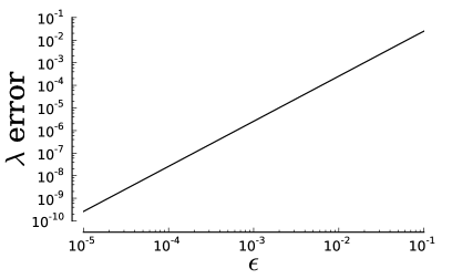
The implicit equation (3.3) can be solved numerically to calculate $\lambda$ to arbitrary precision by a root finding algorithm (e.g., Newton’s method). In Fig. 1 we compute the relative error, $\left|\lambda-\lambda_{\text{\tiny{LT}}}\right|\lambda^{-1}$, of the asymptotic approximation, $\lambda_{\text{\tiny{LT}}}$, as compared to the numerically estimated value of $\lambda$ (computed to machine precision). We see that as $\epsilon\to 0$, the relative error between the two decreases like $\epsilon^{2}$, as expected from (2.11).

Figure 2: (Color online) The spatial density function $p(r,t)$ (black curve) and its asymptotic expansions for small $\epsilon$ at several time points. The blue (light gray) curve gives the leading order expansion (3.16), $p^{(0)}(r,t)$, while the green dashed curve gives the first order expansion (3.12). We use a logarithmic $x$-axis to emphasize the solution behavior near the target. $r_{0}=0.8$ and $\epsilon=0.001$ (similar to the width of measured DNA binding potentials Kühner et al. (2004)).

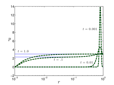
In Fig. 2, we show the leading order spatial density approximation (blue or light gray curve), the first order expansion (green dashed curve), and the exact spatial density (black curve). These curves plot

$$p^{(0)}(r,t)=g(r,r_{0},t)-3+3e^{-\lambda_{\text{\tiny{LT}}}t},$$ (3.16)

the expansion (3.12), and $p(r,t)$ (3.2) respectively. The spatial density is shown as a function of $r$ at four different time points. For this figure we set $r_{0}=0.8$ and $\epsilon=0.001$. The density is initially concentrated around the initial position at $t=0.001$ and slowly fills the region $\epsilon<r<1$ until the density is approximately uniform at $t=1$. The only visible difference between the leading order approximation and the exact result is near the absorbing boundary, $r=\epsilon$, where the exact solution displays a boundary layer that is lost in the leading order approximation. The first order expansion (3.12) reintroduces this boundary layer and is indistinguishable from the exact solution at the scale of the graph.

In the remainder of this section we focus on the approximation of the first passage time. The only free parameters in the model are the radius of the trap, $\epsilon$, and the initial distance from the trap, $r_{0}$. The long time approximation, $f_{\text{\tiny{LT}}}(t)$, is independent of $r_{0}$. It follows that the accuracy of $f_{\text{\tiny{LT}}}(t)$ in approximating $f(t)$ improves when the initial distance from the trap is large (i.e., $\epsilon\ll r_{0}\leq 1$). In other words, the long time approximation is best when the particle is likely to explore a large portion of the domain before locating the trap. When the initial distance from the trap is small (i.e., $\epsilon<r_{0}\ll 1$), we might expect the short time contribution to be significant since there is a higher probability that the particle will quickly locate the trap before exploring the rest of the domain. In Fig. 3, we show the asymptotic expansion of the first passage time density (2.49) for $\epsilon=0.05$ and $r_{0}=0.3$. With this choice the initial distance of the particle from the trap is small. Moreover, since the accuracy of the expansion (2.49) should decrease as $\epsilon$ increases, taking $\epsilon=0.05$ demonstrates the worst case behavior of the expansion for biologically relevant values of $\epsilon$.

Figure 3: (Color online) The first passage time density, $f(t)$, for $r_{0}=0.3$ and $\epsilon=0.05$. Asymptotic approximations of varying order are compared to the exact solution. The left plot uses a logarithmic $t$-axis and linear $f$-axis, while the right is linear in $t$ and logarithmic in $f$.

Figure 4: (Color online) The first passage time density, $f(t)$, for $r_{0}=0.8$ and $\epsilon=0.05$. Asymptotic approximations of varying order are compared to the exact solution. See Fig. 3 (left panel) for the legend.

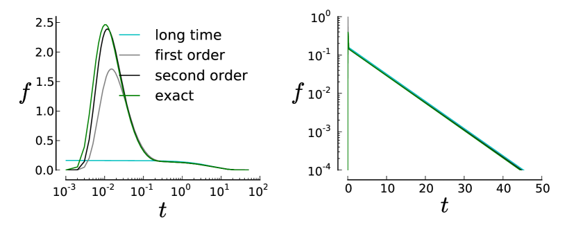
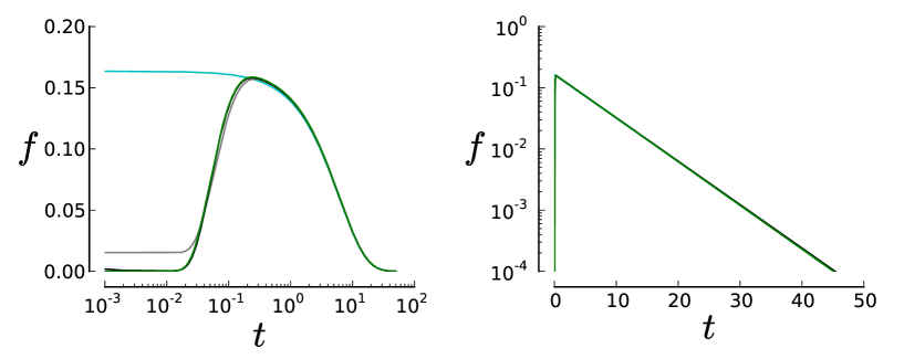
In Fig. 3(left) the density function is shown with $t$ on a log scale to accentuate the small time behavior. There is a significant difference between the long time approximation (near-flat, bottom, light blue curve) and the exact solution (uppermost, green curve). The first and second-order uniform approximations correct for this difference. The large-time behavior is shown in Fig. 3(right) with $f$ on a log scale. For all except the shortest times the curve is linear, reflecting the exponential long-time behavior. We see that on this time-scale there is very little visible difference between each curve. Fig. 4 is the same as Fig. 3, except that $r_{0}=0.8$ so that the initial distance from the trap is larger. In this case the peak in the density occurs at a larger time. In both cases, the qualitative difference between the exact solution and the long-time approximation is a time lag before the exponential long time behavior dominates. The time-scale for this time lag is roughly the diffusive transit time to cover the initial distance from the trap (i.e., $r_{0}^{2}/D$).

Figure 5: (Color online) Absolute error of the first passage time density approximation for $r_{0}=0.3$ and $r_{0}=0.8$ with $\epsilon=0.05$. See Fig. 3 (left panel) for the legend.

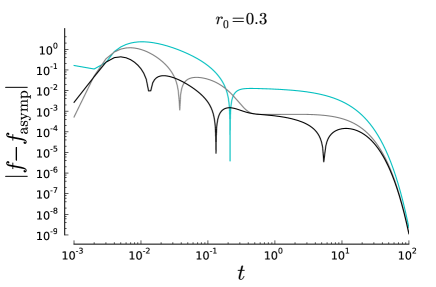
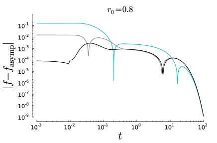
The absolute error of these approximations is shown in Fig. 5 for $r_{0}=0.3$ and $r_{0}=0.8$. In both cases, the maximum error is noticeably decreased as the order of the asymptotic expansion is increased. Comparing the first and second order expansions, we see the main increase in accuracy results for times less than $t=1$. Points in time where one of the approximations crosses the exact solution result in locally increased accuracy (the cusp-like drops in the expansion errors). Interestingly, when $r_{0}=0.8$ the long time approximation is more accurate for large times than the first- or second-order uniform approximations. Note, however, the error in each expansion at these times is substantially smaller than for short to moderate times.

Figure 6: (Color online) The max norm error of the approximation as a function of $\epsilon$. Solid curves show the error of the long-time approximation $f_{\text{\tiny{LT}}}(t)$. The dashed curves show the second order uniform approximation. Note that the $r_{0}=0.65$ and $r_{0}=.9$ curves for the large-time approximation are indistinguishable.

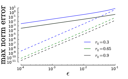
Finally, we examine the max norm error, $\max_{t\geq 0}\left|f_{\rm exact}(t)-f(t)\right|$, as a function of $\epsilon$ for different values of $r_{0}$. The time points this error was numerically evaluated over are the same as those used for the graphs in Fig. 5, and are given in Appendix D. The result shown in Fig. 6 confirms the asymptotic convergence of the approximation as $\epsilon\to 0$. The large-time approximation (2.47) error (solid lines) shows linear convergence, while the second order uniform approximation (2.49) error (dashed line), which includes short time behavior, shows cubic convergence.

As stated in the Introduction, the mean binding time is well approximated by the $r_{0}$-independent large-time approximation. That is, $E[T]\sim 1/\lambda$, where $\lambda$ is given by (2.11). However, other statistics may be of interest that depend strongly on $r_{0}$. One example is the mode, defined as the most likely binding time, call it $\tau_{\rm m}$, where $f(\tau_{\rm m})=\max_{0\leq t<\infty}f(t)$. Since the large-time approximation is an exponential distribution, the corresponding approximation of the mode is $\tau_{\rm m}\sim 0$.

Figure 7: (Color online) The mode of the binding time distribution, defined as the most likely binding time, as a function of $r_{0}$. Solid curves show the exact solution, dash dotted curves the first order approximation, and the dashed curves the 2nd order approximation.

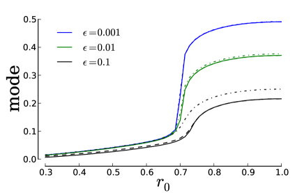
In figure Fig. 7, we compute the mode by numerically maximizing the first passage time density. The exact mode is compared to first (dash dotted curves) and second order (dashed curves) approximations of the mode as a function of $r_{0}$. Each of the indicated curves are drawn for three different values of $\epsilon$. For $\epsilon=10^{-3}$, the difference between each curve is indistinguishable. Notice that as $\epsilon$ decreases the mode increases, particularly for larger values of $r_{0}$, indicating that the large time approximation of the mode becomes less accurate as $\epsilon\to 0$.

IV Discussion

Although the first passage time of a Brownian particle in a confined geometry is a well-studied problem, an analytical characterization that includes short-time behavior of the survival probability density has been unresolved. The asymptotic approximation of the long-time behavior establishes a link between the spatial characteristics of the problem (i.e., the starting position of the particle and the space dependent survival probability density) and the short time behavior. That is, the long time approximation loses information about the initial position and treats the survival probability density as uniform in space. Consequently, the long time approximation is insufficient if one is interested in statistics that depend on these spatial characteristics.

Using a multiple time-scale perturbation approach, we develop a long time expansion and a corresponding short time correction to this expansion of the solution to the diffusion equation in a bounded domain containing a small, absorbing spherical trap. The long time approximation is derived from the matched asymptotic expansions of Ward and Keller (1993), while the short time correction is derived by modification of the pseudopotential method used in Isaacson and Isaacson (2009). Combining these expansions we develop a uniformly accurate (in time) approximation of the survival time cumulative distribution and the first passage time density. To study the accuracy of our method, we consider a example problem where the domain and trap are concentric spheres. By assuming radial symmetry, we have available for comparison the exact solution to the example problem. Our results show excellent quantitative agreement for all times over a range of physiologically realistic values of $\epsilon$. Moreover, they demonstrate the applicability of our expansions to estimating statistics that depend critically on the initial position of the diffusing particle.

Our approach should also be applicable to two-dimensional systems and multiple targets. Pseudopotentials have already been used to approximate rates of diffusion limited reactions in two-dimensional periodic systems Torney and Goldstein (1987). Likewise, pseudopotentials were originally developed to study many-particle scattering problems Huang and Yang (1957); Albeverio et al. (1988); Albeverio and Kurasov (2000). While we are unaware of their use for approximating first passage processes in many-body/target systems, it should be feasible to adapt the techniques previously used in the quantum mechanical scattering context, allowing the extension of our work to multi-target systems.

V Acknowledgments

SAI was supported by NSF grant DMS-0920886. JMN was supported in part by the Mathematical Biosciences Institute and the National Science Foundation under grant DMS-0931642. We thank the referees for their helpful comments and suggestions.

Appendix A Motivation for assumed form of solution to (2.21)

In Berezin and Faddeev (1961); Albeverio et al. (1995, 1988); Albeverio and Kurasov (2000) several approaches for rigorously defining pseudopotential-like interactions are presented (usually called point interactions or singular perturbations of the Laplacian in those works). In the approach of Albeverio et al. (1995); Albeverio and Kurasov (2000); Albeverio et al. (1988), the Laplacian plus point interaction operator, $D\nabla^{2}+\alpha\delta(\bm{r})$, is rigorously constructed so as to be equivalent to the Laplacian with pseudopotential, $D\nabla^{2}-V$ (see (2.17) for the definition of the pseudopotential, $V$, and Albeverio et al. (1988, 1995) for details on the construction of $D\nabla^{2}+\alpha\delta(\bm{r})$). The splitting (2.22) is rigorously justified by these works, and in the context of the diffusion equation goes back at least as far as Dell’Antonio et al. (1998).

We now give a formal motivation for the splitting (2.22) by studying the Laplace transform of (2.21). Again, we refer to the references Albeverio et al. (1995); Albeverio and Kurasov (2000); Albeverio et al. (1988); Dell’Antonio et al. (1998) for the rigorous justification. Our analysis is similar to that given in Section II.A of Grossmann and Wu (1984) (where $\Omega=\mathbb{R}^{3}$). Denote by $\tilde{g}(s)$ the Laplace transform of a function, $g(t)$. Taking the Laplace transform of (2.21) we find

$$-D\nabla^{2}\tilde{p}_{\text{\tiny{ST}}}(\bm{r},s)+s\tilde{p}_{\text{\tiny{ST}}}(\bm{r},s)= -V\tilde{p}_{\text{\tiny{ST}}}(\bm{r},s)+\delta(\bm{r}-\bm{r}_{0})$$

$$-\psi(\bm{r})\psi(\bm{r}_{0}),$$

for $\bm{r}\in\Omega$ and $s>0$, with the Neumann boundary condition that $\partial_{\bm{\eta}}\tilde{p}_{\text{\tiny{ST}}}(\bm{r},s)=0$ for $\bm{r}\in\partial\Omega$. We assume the coefficient of $\delta(\bm{r}-\bm{r}_{\rm{b}})$ within the pseudopotential term is finite, and subsequently denote it by $B(s)$ (as in Grossmann and Wu (1984)),

$$-B(s)\delta(\bm{r}-\bm{r}_{\rm{b}}) \equiv-V\tilde{p}_{\text{\tiny{ST}}}(\bm{r},s)$$

$$=-\epsilon\hat{k}\frac{\partial}{\partial\left|\bm{r}-\bm{r}_{\rm{b}}\right|}\Big{[}\left|\bm{r}-\bm{r}_{\rm{b}}\right|\tilde{p}_{\text{\tiny{ST}}}(\bm{r},s)\Big{]}_{\bm{r}=\bm{r}_{\rm{b}}}$$

$$\phantom{=}\quad\times\delta(\bm{r}-\bm{r}_{\rm{b}}).$$

Recalling that $G(\bm{r},\bm{r}_{0},t)$ is the Green’s function for the $\epsilon=0$ problem (2.4), we may then write

$$\tilde{p}_{\text{\tiny{ST}}}(\bm{r},s) =\tilde{G}(\bm{r},\bm{r}_{0},s)-\psi(\bm{r}_{0})\int_{\Omega}\tilde{G}(\bm{r},\bm{r}^{\prime},s)\psi(\bm{r}^{\prime})d\bm{r}^{\prime}$$

$$\phantom{=}\quad-B(s)\tilde{G}(\bm{r},\bm{r}_{\rm{b}},s)$$

$$=H(\bm{r},s)-B(s)\tilde{G}(\bm{r},\bm{r}_{\rm{b}},s),$$

where $H(\bm{r},s)$ subsequently denotes the first two terms. Substituting the preceding equation for $\tilde{p}_{\text{\tiny{ST}}}(\bm{r},s)$ into the definition of $B(s)$ we find

$$B(s)=\epsilon\hat{k}\left[H(\bm{r}_{\rm{b}},s)-B(s)\left(\tilde{R}(\bm{r}_{\rm{b}},\bm{r}_{\rm{b}},s)-\frac{1}{\hat{k}}\sqrt{\frac{s}{D}}\right)\right].$$

Here we have split $\tilde{G}(\bm{r},\bm{r}^{\prime},s)$ into a part that is regular at $\bm{r}=\bm{r}^{\prime}$, $\tilde{R}(\bm{r},\bm{r}^{\prime},s)$, and an explicit singular part so that

$$\tilde{G}(\bm{r},\bm{r}^{\prime},s)=\tilde{R}(\bm{r},\bm{r}^{\prime},s)+\frac{e^{-\left|\bm{r}-\bm{r}^{\prime}\right|\sqrt{\frac{s}{D}}}}{\hat{k}\left|\bm{r}-\bm{r}^{\prime}\right|}.$$

Solving for $B(s)$ we find

$$B(s)=\frac{\epsilon\hat{k}H(\bm{r}_{\rm{b}},s)}{1+\epsilon\hat{k}\tilde{R}(\bm{r}_{\rm{b}},\bm{r}_{\rm{b}},s)-\epsilon\sqrt{\frac{s}{D}}}.$$

Here we see how the pseudopotential corrects the naive point sink approximation, as given by (2.20). The addition of the radial derivative in the definition of $V$ allows the pseudopotential to remove $r^{-1}$ type singularities in three-dimensions. This allows the unknown coefficient, $B(s)$, to be determined.

Using the last equation for $B(s)$, we find that

$$\tilde{p}_{\text{\tiny{ST}}}(\bm{r},s)=H(\bm{r},s)-\frac{\epsilon\hat{k}H(\bm{r}_{\rm{b}},s)\tilde{G}(\bm{r},\bm{r}_{\rm{b}},s)}{1+\epsilon\hat{k}\tilde{R}(\bm{r}_{\rm{b}},\bm{r}_{\rm{b}},s)-\epsilon\sqrt{\frac{s}{D}}}.$$

We may write

$$\tilde{p}_{\text{\tiny{ST}}}(\bm{r},s)=\tilde{\phi}(\bm{r},s)+\tilde{q}(s)U(\bm{r},\bm{r}_{\rm{b}}),$$ (A.1)

where

$$\tilde{q}(s)=-\frac{\epsilon\hat{k}H(\bm{r}_{\rm{b}},s)}{1+\epsilon\hat{k}\tilde{R}(\bm{r}_{\rm{b}},\bm{r}_{\rm{b}},s)-\epsilon\sqrt{\frac{s}{D}}}$$

and

$$\tilde{\phi}(\bm{r},s)=H(\bm{r},s)+\tilde{q}(s)\left(\tilde{G}(\bm{r},\bm{r}_{\rm{b}},s)-U(\bm{r},\bm{r}_{\rm{b}})\right).$$

As the singular part of $U(\bm{r},\bm{r}_{\rm{b}})$ is $\hat{k}^{-1}\left|\bm{r}-\bm{r}_{\rm{b}}\right|^{-1}$ Cheviakov and Ward (2011), $\tilde{\phi}(\bm{r},s)$ is regular at $\bm{r}=\bm{r}_{\rm{b}}$ for $s>0$. Formally, taking an inverse Laplace transform of (A.1) gives the representation (2.22) of $p_{\text{\tiny{ST}}}(\bm{r},t)$.

Appendix B Limit as $t\to\infty$ of $p_{\text{\tiny{ST}}}^{(2)}$

In this appendix we show that as $t\to\infty$, $p_{\text{\tiny{ST}}}^{(2)}(\bm{r},t)\to 0$ for $\bm{r}\neq\bm{r}_{\rm{b}}$. As in the last appendix, $\tilde{g}(s)$ will denote the Laplace transform of a function, $g(t)$. We first collect some basic identities that will aid in evaluating the limit:

Lemma B.1.

$$\int_{\Omega}w^{(2)}(\bm{r},\bm{r}_{0}\o)d\bm{r} =\hat{k}^{2}\gamma U(\bm{r}_{0},\bm{r}_{\rm{b}})+2\bar{\Psi}\sqrt{\left|\Omega\right|}$$

$$\phantom{=}-\frac{\hat{k}^{2}}{\left|\Omega\right|}\int_{\Omega}U(\bm{r}_{0},\bm{r}^{\prime})U(\bm{r}^{\prime},\bm{r}_{\rm{b}})d\bm{r}^{\prime},$$ (B.1)

$$\int_{\Omega}U(\bm{r}_{0},\bm{r}^{\prime})U(\bm{r}^{\prime},\bm{r}_{\rm{b}})d\bm{r}^{\prime} =\lim_{s\to 0}\frac{U(\bm{r}_{0},\bm{r}_{\rm{b}})-\tilde{\phi}^{(0)}(\bm{r}_{\rm{b}},s)}{s},$$ (B.2)

$$\int_{\Omega}\left(U(\bm{r},\bm{r}_{\rm{b}})\right)^{2}d\bm{r} =\lim_{s\to 0}\int_{\Omega}\tilde{G}(\bm{r}_{\rm{b}},\bm{r}^{\prime},s)U(\bm{r}^{\prime},\bm{r}_{\rm{b}})d\bm{r}^{\prime}.$$ (B.3)

Proof.

The first identity follows immediately from the definition of $w^{(2)}$ (2.15) and (2.8). In the right hand side of (B.2) we replace the $U$ terms with time integrals of $G$ by (2.9), switch the order of integration, and evaluate the spatial integral using the semigroup property of $G$ to find that

$$\int_{\Omega}U(\bm{r}_{0},\bm{r}^{\prime})U(\bm{r}^{\prime},\bm{r}_{\rm{b}})d\bm{r}^{\prime}=\\ \int_{0}^{\infty}\int_{t}^{\infty}\left[G(\bm{r}_{0},\bm{r}_{\rm{b}},s)-\frac{1}{\left|\Omega\right|}\right]dsdt.$$ (B.4)

As

$$\int_{t}^{\infty}\left[G(\bm{r}_{0},\bm{r}_{\rm{b}},s)-\frac{1}{\left|\Omega\right|}\right]ds=\\ U(\bm{r}_{0},\bm{r}_{\rm{b}})-\int_{0}^{t}\left[G(\bm{r}_{0},\bm{r}_{\rm{b}},s)-\frac{1}{\left|\Omega\right|}\right]ds,$$

recalling the definition of $\phi^{(0)}(\bm{r}_{\rm{b}},s)$ (2.35) we see that

$$\int_{\Omega} U(\bm{r}_{0},\bm{r}^{\prime})U(\bm{r}^{\prime},\bm{r}_{\rm{b}})d\bm{r}^{\prime}$$

$$=\int_{0}^{\infty}\left(U(\bm{r}_{0},\bm{r}_{\rm{b}})-\int_{0}^{t}\phi^{(0)}(\bm{r}_{\rm{b}},s^{\prime})ds^{\prime}\right)dt$$

$$=\lim_{s\to 0}\int_{0}^{\infty}\left(U(\bm{r}_{0},\bm{r}_{\rm{b}})-\int_{0}^{t}\phi^{(0)}(\bm{r}_{\rm{b}},s^{\prime})ds^{\prime}\right)e^{-st}dt.$$

(B.2) then follows by definition of the Laplace transform.

Finally, by (2.8) we have that

$$\int_{\Omega}\tilde{G}(\bm{r}_{\rm{b}},\bm{r}^{\prime},s)U(\bm{r}^{\prime},\bm{r}_{\rm{b}})d\bm{r}^{\prime}=\int_{\Omega}\tilde{G}_{0}(\bm{r}_{\rm{b}},\bm{r}^{\prime},s)U(\bm{r}^{\prime},\bm{r}_{\rm{b}})d\bm{r}^{\prime}.$$

Using (2.9), we have that $\lim_{s\to 0}\tilde{G}_{0}(\bm{r}_{\rm{b}},\bm{r}^{\prime},s)=U(\bm{r}_{\rm{b}},\bm{r}^{\prime})$. A dominated convergence argument then implies (B.3). ∎

We are now ready to evaluate the limit of $p_{\text{\tiny{ST}}}^{(2)}(\bm{r},t)$ as $t\to\infty$. By dominated convergence and (2.9), it is immediate from (2.39c) that

$$\lim_{t\to\infty}p_{\text{\tiny{ST}}}^{(2)}(\bm{r},t) =\frac{\hat{k}^{2}\gamma}{\left|\Omega\right|}U(\bm{r}_{\rm{b}},\bm{r}_{0})-\frac{\hat{k}}{\left|\Omega\right|}\int_{0}^{\infty}\phi^{(1)}(\bm{r}_{\rm{b}},s)ds$$

$$\phantom{=}\quad-\frac{1}{\left|\Omega\right|}\int_{\Omega}w^{(2)}(\bm{r}^{\prime},\bm{r}_{0})d\bm{r}^{\prime},$$

$$=-\frac{\hat{k}}{\left|\Omega\right|}\int_{0}^{\infty}\phi^{(1)}(\bm{r}_{\rm{b}},s)ds-\frac{2\bar{\Psi}}{\sqrt{\left|\Omega\right|}}$$

$$\phantom{=}\quad+\frac{\hat{k}^{2}}{\left|\Omega\right|^{2}}\int_{\Omega}U(\bm{r}_{0},\bm{r}^{\prime})U(\bm{r}^{\prime},\bm{r}_{\rm{b}})d\bm{r}^{\prime},$$ (B.5)

where the last line follows by (B.1). By definition of the Laplace transform,

$$\int_{0}^{\infty}\phi^{(1)}(\bm{r}_{\rm{b}},s)ds=\lim_{s\to 0}\lim_{\bm{r}\to\bm{r}_{\rm{b}}}\tilde{\phi}^{(1)}(\bm{r},s).$$

From the definition of $\phi^{(1)}(\bm{r},t)$ (2.36) we find that

$$\tilde{\phi}^{(1)}(\bm{r},s) =\hat{k}\tilde{\phi}^{(0)}(\bm{r}_{\rm{b}},s)\left[U(\bm{r},\bm{r}_{\rm{b}})-\tilde{G}_{0}(\bm{r},\bm{r}_{\rm{b}},s)\right]$$

$$\phantom{=}\quad+\frac{\hat{k}}{\left|\Omega\right|s}\left[U(\bm{r}_{0},\bm{r}_{\rm{b}})-\tilde{\phi}^{(0)}(\bm{r}_{\rm{b}},s)\right]$$

$$\phantom{=}\quad+\frac{\hat{k}}{\left|\Omega\right|}\int_{\Omega}\tilde{G}(\bm{r},\bm{r}^{\prime},s)U(\bm{r}^{\prime},\bm{r}_{\rm{b}})d\bm{r}^{\prime}.$$

Substituting into (B.5), and using (B.2), (B.3), and the definition of $\bar{\Psi}$ (2.13) we find

$$\lim_{t\to\infty}p_{\text{\tiny{ST}}}^{(2)}(\bm{r},t)=-\frac{\hat{k}^{2}U(\bm{r}_{\rm{b}},\bm{r}_{0})}{\left|\Omega\right|}\\ \times\lim_{s\to 0}\lim_{\bm{r}\to\bm{r}_{\rm{b}}}\left[U(\bm{r},\bm{r}_{\rm{b}})-\tilde{G}_{0}(\bm{r},\bm{r}_{\rm{b}},s)\right].$$ (B.6)

The limit of the bracketed term can be evaluated by splitting $U$ and $\tilde{G}_{0}$ into regular and singular parts (at $\bm{r}=\bm{r}_{\rm{b}}$). We write that

$$G_{0}(\bm{r},\bm{r}_{\rm{b}},t)=R_{0}(\bm{r},\bm{r}_{\rm{b}},t)+\frac{1}{\left(4\pi Dt\right)^{3/2}}e^{-\left|\bm{r}-\bm{r}_{\rm{b}}\right|/4Dt},$$

where $R_{0}(\bm{r}_{\rm{b}},\bm{r}_{\rm{b}},t)$ is finite as $t\to 0$. Using (2.9) we see that

$$U(\bm{r},\bm{r}_{\rm{b}})=\tilde{R}_{0}(\bm{r},\bm{r}_{\rm{b}},0)+\frac{1}{\hat{k}\left|\bm{r}-\bm{r}_{\rm{b}}\right|},$$

where $\tilde{R}_{0}(\bm{r},\bm{r}_{\rm{b}},s)$ denotes the Laplace transform of $R$. As such,

$$\lim_{\bm{r}\to\bm{r}_{\rm{b}}}\left[U(\bm{r},\bm{r}_{\rm{b}})-\tilde{G}_{0}(\bm{r},\bm{r}_{\rm{b}},s)\right] =\tilde{R}_{0}(\bm{r}_{\rm{b}},\bm{r}_{\rm{b}},0)$$

$$\phantom{=}-\tilde{R}_{0}(\bm{r}_{\rm{b}},\bm{r}_{\rm{b}},s)+\frac{1}{\hat{k}}\sqrt{\frac{s}{D}}.$$

Evaluating the $s$ limit in (B.6), it follows that as $t\to 0$, $p_{\text{\tiny{ST}}}^{(2)}(\bm{r},t)\to 0$.

Appendix C Spherically-symmetric Neumann Green’s function

Let $g(r,r_{0},t)$ denote the spherically symmetric solution to the diffusion equation, satisfying

$$\frac{\partial g}{\partial t} =D\frac{1}{r^{2}}\frac{\partial}{\partial r}\left[r^{2}\frac{\partial g}{\partial r}\right],\quad r\in\left[0,1\right),$$

$$\frac{\partial g}{\partial r} =0,\quad r=1,$$

with the initial condition that $g(r,r_{0},0)=\delta(r-r_{0})/r^{2}$. With this choice,

$$g(r,r_{0},t)=\iint_{\partial B_{1}(\bm{0})}G(\bm{r},\bm{r}_{0},t)dS,$$

for $\partial B_{1}(\bm{0})$ the boundary of the unit sphere. Here $G(\bm{r},\bm{r}_{0},t)$ denotes the solution to the corresponding three dimensional diffusion equation (2.4). Note also the normalization that

$$\int_{0}^{1}g(r,r_{0},t)r^{2}dr=1=\iiint_{\Omega}G(\bm{r},\bm{r}_{0},t)d\bm{r}.$$

By eigenfunction expansion we find

$$g(r,r_{0},t)=3\\ +2\sum_{n=1}^{\infty}\left(1+\frac{\mu_{n}}{D}\right)\operatorname{sinc}(\sqrt{\frac{\mu_{n}}{D}}r)\operatorname{sinc}(\sqrt{\frac{\mu_{n}}{D}}r_{0})e^{-\mu_{n}t},$$

where the eigenvalues $\mu_{n}$ satisfy (3.11) and we use the convention that

$$\operatorname{sinc}(x)=\frac{\sin(x)}{x}.$$

Appendix D Numerics

When evaluating the series for the exact solution (3.4) and asymptotic approximation (2.49), we sum until the magnitude of the last added term drops below a given error threshold. We used an error threshold of $10^{-14}$ for the exact solution and $10^{-7}$ for the uniform approximation. The figures are generated with 1000 equally-spaced points for $10^{-3}\leq t\leq 1$ and 500 equally-spaced points for $1<t<30$.

References

- Bressloff and Newby (2013) P. C. Bressloff and J. M. Newby, Rev. Mod. Phys. 85, 135 (2013).
- Ward and Keller (1993) M. J. Ward and J. B. Keller, SIAM J. Appl. Math 53, 770 (1993).
- Condamin et al. (2007) S. Condamin, O. Bénichou, and M. Moreau, Phys. Rev. E 75, 021111 (2007).
- Schuss et al. (2007) Z. Schuss, A. Singer, and D. Holcman, PNAS 104, 16098 (2007).
- Coombs et al. (2009) D. Coombs, R. Straube, and M. Ward, SIAM J. Appl. Math. 70, 302 (2009).
- Pillay et al. (2010) S. Pillay, M. J. Ward, A. Peirce, and T. Kolokolnikov, Multiscale Model. Simul. 8, 803 (2010).
- Cheviakov et al. (2010) A. F. Cheviakov, M. J. Ward, and R. Straube, Multiscale Model. Simul. 8, 836 (2010).
- Chevalier et al. (2011) C. Chevalier, O. Bénichou, B. Meyer, and R. Voituriez, Journal of Physics A: Mathematical and Theoretical 44, 025002 (2011).
- Holcman and Schuss (2004) D. Holcman and Z. Schuss, J. Stat. Phys. 117, 975 (2004).
- Bressloff et al. (2007) P. C. Bressloff, B. A. Earnshaw, and M. J. Ward, SIAM J. Appl. Math. 68, 1223 (2007).
- Lagache and Holcman (2007) T. Lagache and D. Holcman, SIAM J. Appl. Math. 68, 1146 (2007).
- Bressloff and Newby (2011) P. C. Bressloff and J. M. Newby, Phys. Rev. E 83, 061139 (2011).
- Isaacson et al. (2011) S. A. Isaacson, D. M. McQueen, and C. S. Peskin, PNAS 108, 3815 (2011).
- Cullen (2003) B. R. Cullen, TRENDS Biochem. Sci. 28, 419 (2003).
- Cheviakov and Ward (2011) A. F. Cheviakov and M. J. Ward, Mathematical and Computer Modelling 53, 1394 (2011).
- Gardiner (1996) C. W. Gardiner, Handbook of Stochastic Methods: For Physics, Chemistry, and the Natural Sciences, 2nd ed., Springer Series in Synergetics, Vol. 13 (Springer Verlag, New York, 1996).
- Van Kampen (2001) N. G. Van Kampen, Stochastic Processes in Physics and Chemistry (North-Holland, Amsterdam, 2001).
- Gardiner et al. (1976) C. W. Gardiner, K. J. McNeil, D. F. Walls, and I. S. Matheson, J. Stat. Phys. 14, 307 (1976).
- Bénichou et al. (2010) O. Bénichou, C. Chevalier, J. Klafter, B. Meyer, and R. Voituriez, Nat. Chem. 2, 472 (2010).
- Mejía-Monasterio et al. (2011) C. Mejía-Monasterio, G. Oshanin, and G. Schehr, J. Stat. Mech.-Theory Exp. 2011, P06022 (2011).
- Mattos et al. (2012) T. G. Mattos, C. Mejía-Monasterio, R. Metzler, and G. Oshanin, Phys. Rev. E 86, 031143 (2012).
- Meyer et al. (2011) B. Meyer, C. Chevalier, R. Voituriez, and O. Bénichou, Phys. Rev. E 83, 051116 (2011).
- Isaacson and Isaacson (2009) S. A. Isaacson and D. Isaacson, Phys. Rev. E 80, 066106 (9pp) (2009).
- Fermi (1936) E. Fermi, Ricerca sci. 7, 13 (1936).
- Huang and Yang (1957) K. Huang and C. N. Yang, Phys. Rev. 105, 767 (1957).
- Torney and Goldstein (1987) D. C. Torney and B. Goldstein, J. Stat. Phys. 49, 725 (1987).
- Berezin and Faddeev (1961) F. Berezin and L. Faddeev, Soviet Math. Dokl. 2, 372 (1961).
- Albeverio et al. (1988) S. Albeverio, F. Gesztesy, R. Høegh-Krohn, and H. Holden, Solvable Models in Quantum Mechanics, 2nd ed. (AMS Chelsea Publishing, Providence, RI, 1988).
- Albeverio et al. (1995) S. Albeverio, Z. Brzeźniak, and L. Da̧browski, J. Funct. Anal. 130, 220 (1995).
- Albeverio and Kurasov (2000) S. Albeverio and P. Kurasov, Singular Perturbations of Differential Operators, London Mathematical Society Lecture Note Series No. 271 (Cambridge University Press, New York, 2000).
- Dell’Antonio et al. (1998) G. F. Dell’Antonio, R. Figari, and A. Teta, Annales de l’Institut Henri Poincaré 69, 413 (1998).
- Carslaw and Jaeger (1959) H. S. Carslaw and J. C. Jaeger, Conduction of heat in solids, 2nd ed. (Clarendon Press, Oxford, 1959).
- Kühner et al. (2004) F. Kühner, L. T. Costa, P. M. Bisch, S. Thalhammer, W. M. Heckl, and H. E. Gaub, Biophys. J. 87, 2683 (2004).
- Grossmann and Wu (1984) A. Grossmann and T. T. Wu, J. Math. Phys. 25, 1742 (1984).