C.P. 66.318, 05315-970 São Paulo, Brazilccinstitutetext: Institut de Physique Théorique,
CEA-Saclay, 91191 Gif-sur-Yvette, Franceddinstitutetext: Instituto de Física Teórica UAM/CSIC,
Calle de Nicolás Cabrera 13-15, E-28049 Madrid, Spain
Sterile neutrino oscillations: the global picture
Abstract
Neutrino oscillations involving eV-scale neutrino mass states are investigated in the context of global neutrino oscillation data including short and long-baseline accelerator, reactor, and radioactive source experiments, as well as atmospheric and solar neutrinos. We consider sterile neutrino mass schemes involving one or two mass-squared differences at the scale denoted by 3+1, 3+2, and 1+3+1. We discuss the hints for eV-scale neutrinos from disappearance (reactor and Gallium anomalies) and appearance (LSND and MiniBooNE) searches, and we present constraints on sterile neutrino mixing from and neutral-current disappearance data. An explanation of all hints in terms of oscillations suffers from severe tension between appearance and disappearance data. The best compatibility is obtained in the 1+3+1 scheme with a p-value of 0.2% and exceedingly worse compatibilities in the 3+1 and 3+2 schemes.
Keywords:
neutrino oscillations, sterile neutrinos1 Introduction
Huge progress has been made in the study of neutrino oscillations Fukuda:1998mi ; Ahmad:2002jz ; Araki:2004mb ; Adamson:2008zt , and with the recent determination of the last unknown mixing angle Abe:2011sj ; Adamson:2011qu ; Abe:2011fz ; An:2012eh ; Ahn:2012nd ; Abe:2012tg a clear first-order picture of the three-flavor lepton mixing matrix has emerged, see e.g. GonzalezGarcia:2012sz . Besides those achievements there are some anomalies which cannot be explained within the three-flavor framework and which might point towards the existence of additional neutrino flavors (so-called sterile neutrinos) with masses at the eV scale:
-
•
The LSND experiment Aguilar:2001ty reports evidence for transitions with , where and are the neutrino energy and the distance between source and detector, respectively.
-
•
This effect is also searched for by the MiniBooNE experiment AguilarArevalo:2007it ; AguilarArevalo:2010wv ; MBnu2012 ; AguilarArevalo:2012va ; Aguilar-Arevalo:2013ara , which reports a yet unexplained event excess in the low-energy region of the electron neutrino and anti-neutrino event spectra. No significant excess is found at higher neutrino energies. Interpreting the data in terms of oscillations, parameter values consistent with the ones from LSND are obtained.
-
•
Radioactive source experiments at the Gallium solar neutrino experiments SAGE and GALLEX have obtained an event rate which is somewhat lower than expected. This effect can be explained by the hypothesis of disappearance due to oscillations with Acero:2007su ; Giunti:2010zu (“Gallium anomaly”).
-
•
A recent re-evaluation of the neutrino flux emitted by nuclear reactors Mueller:2011nm ; Huber:2011wv has led to somewhat increased fluxes compared to previous calculations Schreckenbach:1985ep ; Hahn:1989zr ; VonFeilitzsch:1982jw ; Vogel:1980bk . Based on the new flux calculation, the results of previous short-baseline ( m) reactor experiments are in tension with the prediction, a result which can be explained by assuming disappearance due to oscillations with Mention:2011rk (“reactor anomaly”).
Sterile neutrino oscillation schemes have been considered for a long time, see e.g. GomezCadenas:1995sj ; Goswami:1995yq ; Bilenky:1996rw ; Okada:1996kw for early references on four-neutrino scenarios. Effects of two sterile neutrinos at the eV scale have been considered first in Peres:2000ic ; Sorel:2003hf , oscillations with three sterile neutrinos have been investigated in Maltoni:2007zf ; Conrad:2012qt .
Thus, while the phenomenology of sterile neutrino models is well known, it has also been known for a long time that the LSND and MiniBooNE appearance signals are in tension with bounds from disappearance experiments Maltoni:2002xd ; Strumia:2002fw ; Cirelli:2004cz , challenging an interpretation in terms of sterile neutrino oscillations. This problem remains severe, and in the following we will give a detailed discussion of the status of the appearance hints from LSND and MiniBooNE in the light of recent global data. The situation is better for the hints for disappearance from the reactor and Gallium anomalies, which are not in direct conflict with any other data. This somewhat ambiguous situation asks for an experimental answer, and indeed several projects are under preparation or under investigation, ranging from experiments with radioactive sources, short-baseline reactor experiments, to new accelerator facilities. A recent review on light sterile neutrinos including an overview on possible experimental tests can be found in Abazajian:2012ys .
In this paper we provide an extensive analysis of the present situation of sterile neutrino scenarios. We discuss the possibility to explain the tentative positive signals from LSND and MiniBooNE, as well as the reactor and Gallium anomalies in terms of sterile neutrino oscillations in view of the global data. New ingredients with respect to our previous analysis Kopp:2011qd are the following.
-
•
We use latest data from the MiniBooNE appearance searches MBnu2012 ; AguilarArevalo:2012va ; Aguilar-Arevalo:2013ara . Our MiniBooNE appearance analysis is now based on Monte Carlo events provided by the collaboration taking into account realistic event reconstruction, correlation matrices, as well as oscillations of various background components in a consistent way.
-
•
We include the constraints on the appearance probability from E776 Borodovsky:1992pn and ICARUS Antonello:2012pq .
-
•
We include the Gallium anomaly in our fit.
-
•
We take into account constraints from solar neutrinos, the KamLAND reactor experiment, and LSND and KARMEN measurements of the reaction .
-
•
The treatment of the reactor anomaly is improved and updated by taking into account small changes in the predicted anti-neutrino fluxes as well as an improved consideration of systematic errors and their correlations.
-
•
We take into account charged-current (CC) and neutral-current (NC) data from the MINOS long-baseline experiment Adamson:2010wi ; Adamson:2011ku .
-
•
We include data on disappearance from MiniBooNE AguilarArevalo:2009yj as well as disappearance from a joint MiniBooNE/SciBooNE analysis Cheng:2012yy .
-
•
In our analysis of atmospheric neutrino data, we improve our formalism to fully take into account the mixing of with other active or sterile neutrino states.
All the data used in this work are summarized in Tab. 1. For other recent sterile neutrino global fits see Conrad:2012qt ; Giunti:2011hn ; Archidiacono:2013xxa . We are restricting our analysis to neutrino oscillation data; implications for kinematic neutrino mass measurements and neutrino-less double beta-decay data have been discussed recently in Li:2011ss ; Barry:2011wb ; Giunti:2011cp .
| Experiment | dof | channel | comments |
| Short-baseline reactors | 76 | SBL | |
| Long-baseline reactors | 39 | LBL | |
| KamLAND | 17 | ||
| Gallium | 4 | SBL | |
| Solar neutrinos | 261 | + NC data | |
| LSND/KARMEN C | 32 | SBL | |
| CDHS | 15 | SBL | |
| MiniBooNE | 15 | SBL | |
| MiniBooNE | 42 | SBL | |
| MINOS CC | 20 | LBL | |
| MINOS NC | 20 | LBL | |
| Atmospheric neutrinos | 80 | + NC matter effect | |
| LSND | 11 | SBL | |
| KARMEN | 9 | SBL | |
| NOMAD | 1 | SBL | |
| MiniBooNE | 11 | SBL | |
| MiniBooNE | 11 | SBL | |
| E776 | 24 | SBL | |
| ICARUS | 1 | LBL | |
| total | 689 | ||
Sterile neutrinos at the eV scale also have implications for cosmology. If thermalized in the early Universe they contribute to the number of relativistic degrees of freedom (effective number of neutrino species ). A review with many references can be found in Abazajian:2012ys . Indeed there might be some hints from cosmology for additional relativistic degrees of freedoms ( bigger than 3), coming mainly from CMB data, e.g. Hamann:2010bk ; Giusarma:2011ex ; GonzalezGarcia:2010un ; Archidiacono:2012ri ; NeffLunardini:2013 ; Archidiacono:2013xxa . Recently precise CMB data from the PLANCK satellite have been released Ade:2013zuv . Depending on which additional cosmological data are used, values ranging from to (uncertainties at 95% CL) are obtained Ade:2013zuv . Constraints from Big Bang Nucleosynthesis on have been considered recently in Mangano:2011ar . Apart from their contribution to , thermalized eV-scale neutrinos would also give a large contribution to the sum of neutrino masses, which is constrained to be below around 0.5 eV. The exact constraint depends on which cosmological data sets are used, but the most important observables are those related to galaxy clustering Hamann:2010bk ; Giusarma:2011ex ; GonzalezGarcia:2010un ; Archidiacono:2012ri . In the standard CDM cosmology framework the bound on the sum of neutrino masses is in tension with the masses required to explain the aforementioned terrestrial hints Archidiacono:2012ri . The question to what extent such sterile neutrino scenarios are disfavored by cosmology and how far one would need to deviate from the CDM model in order to accommodate them remains under discussion Hamann:2011ge ; Joudaki:2012uk ; Archidiacono:2013xxa . We will not include any information from cosmology explicitly in our numerical analysis. However, we will keep in mind that neutrino masses in excess of few eV may become more and more difficult to reconcile with cosmological observations.
The outline of the paper is as follows. In Sec. 2 we introduce the formalism of sterile neutrino oscillations and fix the parametrization of the mixing matrix. We then consider disappearance data in Sec. 3, discussing the reactor and Gallium anomalies. Constraints from disappearance as well as neutral-current data are discussed in Sec. 4, and global appearance data including the LSND and MiniBooNE signals in Sec. 5. The global fit of all these data combined is presented in Sec. 6 for scenarios with one or two sterile neutrinos. We summarize our results and conclude in Sec. 7. Supplementary material is provided in the appendices including a discussion of complex phases in sterile neutrino oscillations, oscillation probabilities for solar and atmospheric neutrinos, as well as technical details of our experiment simulations.
2 Oscillation parameters in the presence of sterile neutrinos
In this work we consider the presence of or 2 additional neutrino states with masses in the few eV range. When moving from 1 to 2 sterile neutrinos the qualitative new feature is the possibility of CP violation already at short-baseline Karagiorgi:2006jf ; Maltoni:2007zf .111Adding more than two sterile neutrinos does not lead to any qualitatively new physical effects and as shown in Maltoni:2007zf the fit does not improve significantly. Therefore, we restrict the present analysis to sterile neutrinos. The neutrino mass eigenstates are labeled such that , , contribute mostly to the active flavor eigenstates and provide the mass squared differences required for “standard” three-flavor oscillations, and , where . The mass states , are mostly sterile and provide mass-squared differences in the range . In the case of only one sterile neutrino, denoted by “3+1” in the following, we always assume , but the oscillation phenomenology for would be the same. For two sterile neutrinos, we distinguish between a mass spectrum where and are both positive (“3+2”) and where one of them is negative (“1+3+1”). The phenomenology is slightly different in the two cases Goswami:2007kv . We assume that the linear combinations of mass states which are orthogonal to the three flavor states participating in weak interactions are true singlets and have no interaction with Standard Model particles. Oscillation physics is then described by a rectangular mixing matrix with and , and .222In this work we consider so-called phenomenological sterile neutrino models, where the neutrino mass eigenvalues and the mixing parameters are considered to be completely independent. In particular we do not assume a seesaw scenario, where the Dirac and Majorana mass matrices of the sterile neutrinos are the only source of neutrino mass and mixing. For such “minimal” sterile neutrino models see e.g. Blennow:2011vn ; Fan:2012ca ; Donini:2012tt .
We give here expressions for the oscillation probabilities in vacuum, focusing on the 3+2 case. It is trivial to recover the 3+1 formulas from them by simply dropping all terms involving the index “5”. Formulas for the 1+3+1 scenario are obtained by taking either or negative. Oscillation probabilities relevant for solar and atmospheric neutrinos are given in appendices C and D, respectively.
First we consider the so-called “short-baseline” (SBL) limit, where the relevant range of neutrino energies and baselines is such that effects of and can be neglected. Then, oscillation probabilities depend only on and with . We obtain for the appearance probability
| (1) |
with the definitions
| (2) |
Eq. (1) holds for neutrinos; for anti-neutrinos one has to replace . Since Eq. (1) is invariant under the transformation and , we can restrict the parameter range to , or equivalently , without loss of generality. Note also that the probability Eq. (1) depends only on the combinations and . The only SBL appearance experiments we are considering are in the channel. Therefore, the total number of independent parameters is 5 if only SBL appearance experiments are considered.
The 3+2 survival probability, on the other hand, is given in the SBL approximation by
| (3) |
In this work we include also experiments for which the SBL approximation cannot be adopted, in particular MINOS and ICARUS. For these experiments is of order one. In the following we give the relevant oscillation probabilities in the limit of and . We call this the long-baseline (LBL) approximation. In this case we obtain for the neutrino appearance probability ()
| (4) |
The corresponding expression for anti-neutrinos is obtained by the replacement . The survival probability in the LBL limit can be written as
| (5) |
Note that in the numerical analysis of MINOS data neither the SBL nor the LBL approximations can be used because , and can all become of order one either at the far detector or at the near detector Hernandez:2011rs . Moreover, matter effects cannot be neglected in MINOS. All of these effects are properly included in our numerical analysis of the MINOS experiment.
Sometimes it is convenient to complete the rectangular mixing matrix by rows to an unitary matrix, with . For we use the following parametrization for :
| (6) |
where represents a real rotation matrix by an angle in the plane, and represents a complex rotation by an angle and a phase . The particular ordering of the rotation matrices is an arbitrary convention which, however, turns out to be convenient for practical reasons.333Note that the ordering chosen in Eq. (6) is equivalent to , where the standard three-flavor convention appears to the right (apart from an additional complex phase), and mixing involving the mass states and appear successively to the left of it. We have dropped the unobservable rotation matrix which just mixes sterile states. There is also some freedom regarding which phases are removed by field redefinitions and which ones are kept as physical phases. In appendix A we give a specific recipe for how to remove unphysical phases in a consistent way. Throughout this work we consider only phases which are phenomenologically relevant in neutrino oscillations. Under certain approximations, more phases may become unphysical. For instance, if an angle which corresponds to a rotation which can be chosen to be complex is zero the corresponding phase disappears. In practical situations often one or more of the mass-squared differences can be considered to be zero, which again implies that some of the angles and phases will become unphysical. In Tab. 2 we show the angle and phase counting for the SBL and LBL approximations for the 3+2 and 3+1 cases.
| A/P | LBL approx. | (A/P) | SBL approx. | (A/P) | |
|---|---|---|---|---|---|
| 3+2 | 9/5 | (8/4) | (6/2) | ||
| 3+1 | 6/3 | (5/2) | (3/0) |
In the notation of Eqs. (1), (3), (4), (5), it is explicit that only appearance experiments depend on complex phases in a parametrization independent way. However, in a particular parametrization such as Eq. (6), also the moduli may depend on cosines of the phase parameters , leading to some sensitivity of disappearance experiments to the in a CP-even fashion. Our parametrization Eq. (6) guarantees that disappearance experiments are independent of .
3 and disappearance searches
Disappearance experiments in the sector probe the moduli of the entries in the first row of the neutrino mixing matrix, . In the short-baseline limit of the 3+1 scenario, the only relevant parameter is . For two sterile neutrinos, also is relevant. In this section we focus on 3+1 models, and comment only briefly on 3+2. For 3+1 oscillations in the SBL limit, the survival probability takes an effective two flavor form
| (7) |
where we have defined an effective -disappearance mixing angle by
| (8) |
This definition is parametrization independent. Using the specific parametrization of Eq. (6) it turns out that .
3.1 SBL reactor experiments
| experiment | [m] | obs/pred | unc. error [%] | tot. error [%] |
|---|---|---|---|---|
| Bugey4 Declais:1994ma | 15 | 0.926 | 1.09 | 1.37 |
| Rovno91 Kuvshinnikov:1990ry | 18 | 0.924 | 2.10 | 2.76 |
| Bugey3 Declais:1994su | 15 | 0.930 | 2.05 | 4.40 |
| Bugey3 Declais:1994su | 40 | 0.936 | 2.06 | 4.41 |
| Bugey3 Declais:1994su | 95 | 0.861 | 14.6 | 1.51 |
| Gosgen Zacek:1986cu | 38 | 0.949 | 2.38 | 5.35 |
| Gosgen Zacek:1986cu | 45 | 0.975 | 2.31 | 5.32 |
| Gosgen Zacek:1986cu | 65 | 0.909 | 4.81 | 6.79 |
| ILL Kwon:1981ua | 9 | 0.788 | 8.52 | 1.16 |
| Krasnoyarsk Vidyakin:1987ue | 33 | 0.920 | 3.55 | 6.00 |
| Krasnoyarsk Vidyakin:1987ue | 92 | 0.937 | 19.8 | 2.03 |
| Krasnoyarsk Vidyakin:1994ut | 57 | 0.931 | 2.67 | 4.32 |
| SRP Greenwood:1996pb | 18 | 0.936 | 1.95 | 2.79 |
| SRP Greenwood:1996pb | 24 | 1.001 | 2.11 | 2.90 |
| Rovno88 Afonin:1988gx | 18 | 0.901 | 4.24 | 6.38 |
| Rovno88 Afonin:1988gx | 18 | 0.932 | 4.24 | 6.38 |
| Rovno88 Afonin:1988gx | 18 | 0.955 | 4.95 | 7.33 |
| Rovno88 Afonin:1988gx | 25 | 0.943 | 4.95 | 7.33 |
| Rovno88 Afonin:1988gx | 18 | 0.922 | 4.53 | 6.77 |
| Palo Verde Boehm:2001ik | 820 | 1 rate | ||
| Chooz Apollonio:2002gd | 1050 | 14 bins | ||
| DoubleChooz Abe:2012tg | 1050 | 18 bins | ||
| DayaBay DBneutrino | 6 rates – 1 norm | |||
| RENO Ahn:2012nd | 2 rates – 1 norm | |||
| KamLAND Gando:2010aa | 17 bins | |||
The data from reactor experiments used in our analysis are summarized in Tab. 3. Our simulations make use of a dedicated reactor code based on previous publications, see e.g. Grimus:2001mn ; Schwetz:2011qt . We have updated the code to include the latest data and improved the treatment of uncertainties, see appendix B for details. The code used here is very similar to the one from Ref. GonzalezGarcia:2012sz , extended to sterile neutrino oscillations. The reactor experiments listed in Tab. 3 can be divided into short-baseline (SBL) experiments with baselines m, long-baseline (LBL) experiments with , and the very long-baseline experiment KamLAND with an average baseline of 180 km. SBL experiments are not sensitive to standard three-flavor oscillations, but can observe oscillatory behavior for , . On the other hand, for long-baseline experiments, oscillations due to , are most relevant, and oscillations due to -scale mass-squared differences are averaged out and lead only to a constant flux suppression. KamLAND is sensitive to oscillations driven by and , whereas all with lead only to a constant flux reduction.
For the SBL reactor experiments we show in Tab. 3 also the ratio of the observed and predicted rate, where the latter is based on the flux calculations of Huber:2011wv for neutrinos from 235U, 239Pu, 241Pu fission and Mueller:2011nm for 238U fission. The ratios are taken from Abazajian:2012ys (which provides and update of Mention:2011rk ) and are based on the Particle Data Group’s 2011 value for the neutron lifetime, s Nakamura:2010zzi .444This number differs from their 2012 value 880.1 s by less than 0.2% pdg . The neutron lifetime enters the calculation of the detection cross section and therefore has a direct impact on the expected rate. The quoted uncertainties of are small compared to the uncertainties on the predicted flux, see RevModPhys.83.1173 for a discussion of the neutron lifetime determination. We observe that most of the ratios are smaller than one. In order to asses the significance of this deviation, a careful error analysis is necessary. In the last column of Tab. 3, we give the uncorrelated errors on the rates. They include statistical as well as uncorrelated experimental errors. In addition to these, there are also correlated experimental errors between various data points which are described in detail in appendix B. Furthermore, we take into account the uncertainty on the neutrino flux prediction following the prescription given in Huber:2011wv , see also appendix B for details.
Fitting the SBL data to the predicted rates we obtain which corresponds to a -value of 2.4%. When expressed in terms of an energy-independent normalization factor , the best fit is obtained at
| (9) |
Here denotes the improvement in compared to a fit with . Clearly the -value increases drastically when is allowed to float, leading to a preference for at the confidence level. This is our result for the significance of the reactor anomaly. Let us mention that (obviously) this result depends on the assumed systematic errors. While we have no particular reason to doubt any of the quoted errors, we have checked that when an adhoc additional normalization uncertainty of 2% (3%) is added, the significance is reduced to (). This shows that the reactor anomaly relies on the control of systematic errors at the percent level.
| /dof (GOF) | /dof (CL) | |||
|---|---|---|---|---|
| SBL rates only | 0.13 | 0.44 | 11.5/17 (83%) | 11.4/2 (99.7%) |
| SBL incl. Bugey3 spectr. | 0.10 | 1.75 | 58.3/74 (91%) | 9.0/2 (98.9%) |
| SBL + Gallium | 0.11 | 1.80 | 64.0/78 (87%) | 14.0/2 (99.9%) |
| SBL + LBL | 0.09 | 1.78 | 93.0/113 (92%) | 9.2/2 (99.0%) |
| global disapp. | 0.09 | 1.78 | 403.3/427 (79%) | 12.6/2 (99.8%) |
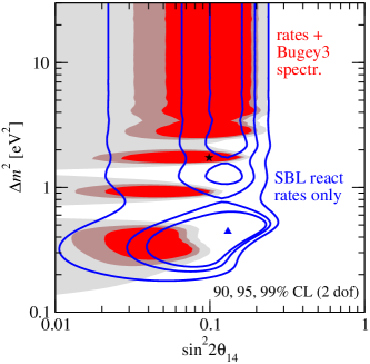
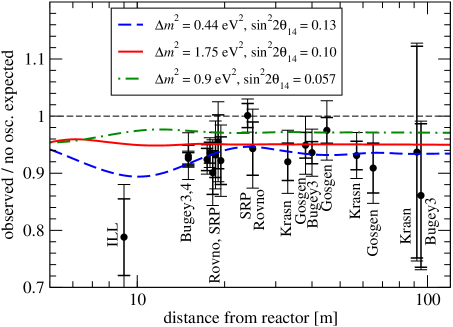
The flux reduction suggested by the reactor anomaly can be explained by sterile neutrino oscillations. In Tab. 4 we give the best fit points and values obtained by fitting SBL reactor data in a 3+1 framework. The allowed regions in and are shown in Fig. 1 (left) for a rate-only analysis as well as a fit including also Bugey3 spectral data. Both analyses give consistent results, with the main difference being that the spectral data disfavors certain values of around and 1.3 . The right panel of Fig. 1 shows the predicted rate suppression as a function of the baseline compared to the data. We show the prediction for the two best fit points from the left panel as well as one point located in the island around , which will be important in the combined fit with SBL appearance data. We observe that for the rate-only best fit point with the prediction follows the tendency suggested by the ILL, Bugey4, and SRP (24 km) data points. This feature is no longer present for , somewhat preferred by Bugey3 spectral data, where oscillations happen at even shorter baselines. However, from the GOF values given in Tab. 4 we conclude that also those solutions provide a good fit to the data.
3.2 The Gallium anomaly
The response of Gallium solar neutrino experiments has been tested by deploying radioactive 51Cr or 37Ar sources in the GALLEX Hampel:1997fc ; Kaether:2010ag and SAGE Abdurashitov:1998ne ; Abdurashitov:2005tb detectors. Results are reported as ratios of observed to expected rates, where the latter are traditionally computed using the best fit cross section from Bahcall Bahcall:1997eg , see e.g. Giunti:2010zu . The values for the cross sections weighted over the 4 (2) neutrino energy lines from Cr (Ar) from Bahcall:1997eg are , . While the cross section for into the ground state of is well known from the inverse reaction there are large uncertainties when the process proceeds via excited states of 71Ge at 175 and 500 keV. Following Bahcall:1997eg , the total cross section can be written as
| (10) |
with , Ar. The coefficients , , , are phase space factors. The ground state cross sections are precisely known Bahcall:1997eg : , . BGT denote the Gamov-Teller strength of the transitions, which have been determined recently by dedicated measurements Frekers:2011zz as
| (11) |
In our analysis we use these values together with Eq. (10) for the cross section.
This means that the ratios of observed to expected rates based on the Bahcall prediction have to be rescaled by a factor 0.982 (0.977) for the Cr (Ar) experiments, so that we obtain for them the following updated numbers for our fits:
| (12) |
Here, we have symmetrized the errors, and we have included only experimental errors, but not the uncertainty on the cross section (see below).
We build a out of the four data points from GALLEX and SAGE and introduce two pulls corresponding to the systematic uncertainty of the two transitions to excited state according to Eq. (11). The determination of BGT175 is relatively poor, with zero being allowed at . In order to avoid unphysical negative contributions from the 175 keV state, we restrict the domain of the corresponding pull parameter accordingly. Fitting the four data points with a constant neutrino flux normalization factor we find
| (13) |
Because of the different cross sections used, these results differ from the ones obtained in Giunti:2010zu , where the best fit point is at , while the significance is comparable, around . An updated analysis including also a discussion of the implications of the measurement in Frekers:2011zz can be found in Giunti:2012tn .
The event deficit in radioactive source experiments can be explained by assuming mixing with an eV-scale state, such that disappearance happens within the detector volume Acero:2007su . We fit the Gallium data in the 3+1 framework by averaging the oscillation probability over the detector volume using the geometries given in Acero:2007su . The resulting allowed region at 95% confidence level is shown in orange in Fig. 2. Consistent with the above discussion we find mixing angles somewhat smaller than those obtained by the authors of Giunti:2010zu . The best fit point from combined Gallium+SBL reactor data is given in Tab. 4, and the no-oscillation hypothesis is disfavored at 99.9% CL (2 dof) or compared to the 3+1 best fit point.
| (GOF) | (CL) | (CL) | |||||
|---|---|---|---|---|---|---|---|
| SBLR | 0.46 | 0.87 | 0.12 | 0.13 | 53.0/(76-4) (95%) | 5.3 (93%) | 14.3 (99.3%) |
| SBLR+gal | 0.46 | 0.87 | 0.12 | 0.14 | 60.2/(80-4) (90%) | 3.8 (85%) | 17.8 (99.9%) |
Let us consider now the Gallium and SBL reactor data in the framework of two sterile neutrinos, in particular in the 3+2 scheme. SBL and disappearance data depend on 4 parameters in this case, , , and the two mixing angles and (or, equivalently, the moduli of the two matrix elements and ). We report the best fit points from SBL reactor data and from SBL reactor data combined with the Gallium source data in Tab. 5. For these two cases we find an improvement of 5.3 and 3.8 units in , respectively, when going from the 3+1 scenario to the 3+2 case. Considering that the 3+2 model has two additional parameters compared to 3+1, we conclude that there is no improvement of the fit beyond the one expected by increasing the number of parameters, and that SBL data sets show no significant preference for 3+2 over 3+1. This is also visible from the fact that the confidence level at which the no oscillation hypothesis is excluded does not increase for 3+2 compared to 3+1, see the last columns of Tabs. 4 and 5. There the is translated into a confidence level by taking into account the number of parameters relevant in each model, i.e., 2 for 3+1 and 4 for 3+2.
3.3 Global data on and disappearance
Let us now consider the global picture regarding disappearance. In addition to the short-baseline reactor and Gallium data discussed above, we now add data from the following experiments:
-
•
The remaining reactor experiments at a long baseline (“LBL reactors”) and the very long-baseline reactor experiment KamLAND, see table 3.
-
•
Global data on solar neutrinos, see appendix C for details.
-
•
LSND and KARMEN measurements of the reaction Auerbach:2001hz ; Armbruster:1998uk . The experiments have found agreement with the expected cross section Fukugita:1988hg , hence their measurements constrain the disappearance of with eV-scale mass-squared differences Reichenbacher:2005nc ; Conrad:2011ce . Details on our analysis of the scattering data are given in appendix E.1.
So far the LBL experiments DayaBay and RENO have released only data on the relative comparison of near ( m) and far ( km) detectors, but no information on the absolute flux determination is available. Therefore, their published data are essentially insensitive to oscillations with eV-scale neutrinos and they contribute only indirectly via constraining . In our analysis we include a free, independent flux normalization factor for each of those two experiments. Chooz and DoubleChooz both lack a near detector. Therefore, in the official analyses performed by the respective collaborations the Bugey4 measurement is used to normalize the flux. This makes the official Chooz and DoubleChooz results on also largely independent of the presence of sterile neutrinos. However, the absolute rate of Bugey4 in terms of the flux predictions is published (see Tab. 3) and we can use this number to obtain an absolute flux prediction for Chooz and DoubleChooz. Therefore, in our analysis Chooz and DoubleChooz (as well as Palo Verde) by themselves also show some sensitivity to sterile neutrino oscillations. In a combined analysis of Chooz and DoubleChooz with SBLR data the official analyses are recovered approximately. Previous considerations of LBL reactor experiments in the context of sterile neutrinos can be found in Refs. Bandyopadhyay:2007rj ; Bora:2012pi ; Giunti:2011vc ; Bhattacharya:2011ee .
We show in Tab. 4 a combined analysis of the SBL and LBL reactor experiments (row denoted by “SBL+LBL”), where we minimize with respect to . We find that the significance of the reactor anomaly is not affected by the inclusion of LBL experiments and finite . The even slightly increases from 9.0 to 9.2 when adding LBL data to the SBL data (“no-osc” refers here to ). Hence, we do not agree with the conclusions of Ref. Zhang:2013ela , which finds that the significance of the reactor anomaly is reduced to when LBL data and a finite value of is taken into account.
Solar neutrinos are also sensitive to sterile neutrino mixing (see e.g. Giunti:2009xz ; Palazzo:2011rj ; Palazzo:2012yf ). The main effect of the presence of mixing with eV states is an over-all flux reduction. While this effect is largely degenerate with , a non-trivial bound is obtained in the combination with DayaBay, RENO and KamLAND. KamLAND is sensitive to oscillations driven by and , whereas sterile neutrinos affect the overall normalization, degenerate with . The matter effect in the sun as well as SNO NC data provide additional signatures of sterile neutrinos, beyond an overall normalization. As we will show in Sec. 4 solar data depend also on the mixing angles and , controlling the fraction of transitions, see e.g. Giunti:2009xz . As discussed in appendix C, in the limit for , solar data depends on 6 real mixing parameters, 1 complex phase and . Hence, in a 3+1 scheme all six mixing angles are necessary to describe solar data in full generality. However, once other constraints on mixing angles are taken into account the effect of , , and the complex phase are tiny and numerically have a negligible impact on our results. Therefore we set for the solar neutrino analysis in this section. In this limit solar data becomes also independent of the complex phase.
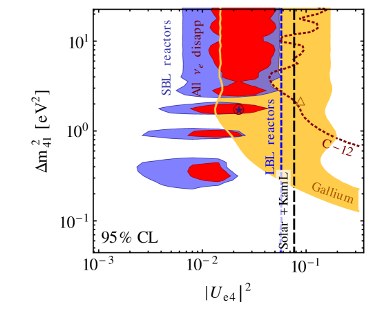
The results of our fit to global disappearance data are shown in Fig. 2 and the best fit point is given in Tab. 4. For this analysis the mass-squared differences and have been fixed, whereas we marginalize over the mixing angles and . We see from Fig. 2 that the parameter region favored by short-baseline reactor and Gallium data is well consistent with constraints from long-baseline reactors, KARMEN’s and LSND’s rate, and with solar and KamLAND data.
Recently, data from the Mainz Kraus:2012he and Troitsk Belesev:2012hx tritium beta-decay experiments have been re-analyzed to set limits on the mixing of with new eV neutrino mass states. Taking the results of Belesev:2012hx at face value, the Troitsk limit would cut-off the high-mass region in Fig. 2 at around 100 Giunti:2012bc (above the plot-range shown in the figure). The bounds obtained in Kraus:2012he are somewhat weaker. The differences between the limits obtained in Kraus:2012he and Belesev:2012hx depend on assumptions concerning systematic uncertainties and therefore we prefer not to explicitly include them in our fit. The sensitivity of future tritium decay data from the KATRIN experiment has been estimated in Riis:2010zm . Implications of sterile neutrinos for neutrino-less double beta-decay have been discussed recently in Li:2011ss ; Barry:2011wb ; Giunti:2011cp .

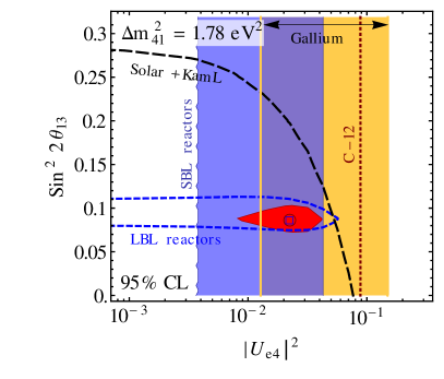
Let us now address the question whether the presence of a sterile neutrino affects the determination of the mixing angle (see also Bhattacharya:2011ee ; Zhang:2013ela ). In Fig. 3 we show the combined determination of and for two fixed values of . The left panel corresponds to a relatively large value of 10 , whereas for the right panel we have chosen the value favored by the global disappearance best fit point, 1.78 . The mass-squared differences and have been fixed, whereas we marginalize over the mixing angle . We observe a clear complementarity of the different data sets: SBL reactor and Gallium data determine , since oscillations are possible only via , all other mass-squared differences are effectively zero for them. For LBL reactors can be set to infinity, is finite, and is effectively zero; therefore they provide an unambiguous determination of by comparing near and far detector data. The upper bound on from LBL reactors is provided by Chooz, Palo Verde, DoubleChooz, since for those experiments also information on the absolute flux normalization can be used, as mentioned above. In contrast, for solar neutrinos and KamLAND, both and are effectively infinite, and and affect essentially the overall normalization and are largely degenerate, as visible the figure.
In conclusion, the determination is rather stable with respect to the presence of sterile neutrinos. We note, however, that its interpretation becomes slightly more complicated. For instance, in the 3+1 scheme using the parametrization from Tab. 2, the relation between mixing matrix elements and mixing angles is and . Hence, the one-to-one correspondence between and as in the three-flavor case is spoiled.
4 , , and neutral-current disappearance searches
In this section we discuss the constraints on the mixing of and with new eV-scale mass states. In the 3+1 scheme this is parametrized by and , respectively. In terms of the mixing angles as defined in Eq. (6) we have and . In the present paper we include data sets from the following experiments to constrain and mixing with eV states:
-
•
SBL disappearance data from CDHS Dydak:1983zq . Details of our simulation are given in Grimus:2001mn .
-
•
Super-Kamiokande. It has been pointed out in Bilenky:1999ny that atmospheric neutrino data from Super-Kamiokande provide a bound on the mixing of with eV-scale mass states, i.e., on the mixing matrix elements , . In addition, neutral-current matter effects provide a constraint on , . A discussion of the effect is given in the appendix of Maltoni:2007zf . Details on our analysis and references are given in appendix D.
-
•
MiniBooNE AguilarArevalo:2009yj ; Cheng:2012yy . Apart from the appearance search, MiniBooNE can also look for SBL disappearance. Details on our analysis are given in appendix E.4.
-
•
MINOS Adamson:2010wi ; Adamson:2011ku . The MINOS long-baseline experiment has published data on charged current (CC) disappearance as well as on the neutral current (NC) count rate. Both are based on a comparison of near and far detector measurements. In addition to providing the most precise determination of (from CC data), those data can also be used to constrain sterile neutrino mixing, where CC (NC) data are mainly relevant for , (, ). See appendix E.5 for details.
Additional constrains on mixing with eV-scale states (not used in this analysis) can be obtained from data from the Ice Cube neutrino telescope Nunokawa:2003ep ; Choubey:2007ji ; Razzaque:2011ab ; Barger:2011rc ; Razzaque:2012tp ; Esmaili:2012nz .

Limits on the row of the mixing matrix come from disappearance experiments. In a 3+1 scheme the SBL disappearance probability is given by
| (14) |
where we have defined an effective disappearance mixing angle by
| (15) |
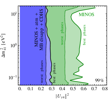
i.e., in our parametrization (6) the effective mixing angle depends on both and . In contrast to the disappearance searches discussed in the previous section, experiments probing disappearance have not reported any hints for a positive signal. We show the limits from the data listed above in the left panel of Fig. 4. Note that the MINOS limit is based on the comparison of the data in near and far detectors. For oscillation effects become relevant at the near detector, explaining the corresponding features in the MINOS bound around that value of , whereas the features around emerge from oscillation effects in the far detector. The roughly constant limit in the intermediate range corresponds to the limit in the near (far) detector adopted in Adamson:2010wi ; Adamson:2011ku . In that range the MINOS limit on is comparable to the one from SuperK atmospheric data. For the limit is dominated by CDHS and MiniBooNE disappearance data.
In Fig. 4 (left) we show also the region preferred by the hints for eV-scale oscillations from LSND and MiniBooNE appearance data (see next section) combined with reactor and Gallium data on disappearance. For fixed we minimize the corresponding with respect to to show the projection in the plane of and . The tension between the hints in the and channels compared to the limits from data is clearly visible in this plot. We will discuss this conflict in detail in section 6.
Limits on the mixing of with eV-scale states are obtained from data involving information from NC interactions, which allow to distinguish between and transitions.555The searches for appearance at NOMAD Astier:2001yj and CHORUS Eskut:2007rn at short baselines are sensitive only to specific parameter combinations like or and therefore do not provide a constraint on by itself. The relevant data samples are atmospheric and solar neutrinos (via the NC matter effect) and MINOS NC data. Furthermore, the parameter controls the relative weight of the oscillation modes and at the “atmospheric” scale : a large value of implies a large fraction of oscillations at the scale. The limit in the plane of and is shown in the right panel of Fig. 4.
As follows from Eq. (4) (see also appendix A), in the LBL approximation relevant for MINOS NC data a complex phase enters the oscillation probabilities, corresponding to the combination . In our calculations we take the rotation matrix to be complex and use the phase to parametrize this phase. In Fig. 4 we illustrate the impact of this phase by showing the strongest and weakest limit obtained when varying . We observe that the limit from MINOS depends quite significantly on this phase. The different shapes of the “best phase” and “worst phase” regions emerge from the different properties of CC and NC data. For the weakest limit (“best phase”) the fit uses the freedom of the term including the complex phase, which implies that a finite value of (or ) is adopted, subject to the constraint from MINOS CC data. Therefore the same structure as in the left panel of Fig. 4 becomes visible also in limit on . If we force the phase to take on a value not favored by the fit, a smaller is obtained for close to zero, which implies that the phase actually becomes unphysical. In this case CC data are not important for the limit on , which then is dominated by NC data. Because of the much worse energy reconstruction for NC events compared to CC ones, the features induced by finite values of in either the far or near detector become to a large extent washed out.
The global limit on is actually dominated by atmospheric neutrino data and shows only a very weak dependence on the complex phase. In our atmospheric neutrino analysis the information on enters via the NC matter effect induced by the presence of sterile neutrinos. A large value of would imply a significant matter effect in driven disappearance, which is not consistent with the zenith angle distribution observed in SuperK. We find the limit
| (16) |
from global data, largely independent of as well as complex phases.
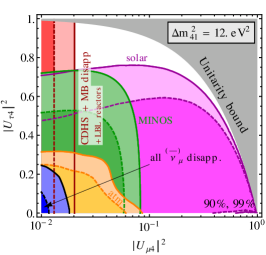

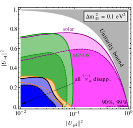
Fig. 5 shows the constraints in the plane of and for three fixed values of . We observe the comparable bound on from MINOS (mainly CC data) and atmospheric, which however is superseded by CDHS, MiniBooNE for (left and middle panels). Those latter data however, do not provide any constraint on , where the global bound is dominated by atmospheric neutrinos for all values of of interest. We also observe that solar neutrinos provide a bound on of similar strength as MINOS data, thanks to the NC matter effect and SNO NC data. No relevant limit can be set on from solar neutrinos.
5 and appearance searches
Now we move on to the discussion of appearance searches. In contrast to disappearance experiments which probe only one row of the mixing matrix, i.e., only the elements for fixed , an appearance experiment in the channel is sensitive to two rows via combinations like and potentially to some complex phases. In the SBL approximation the 3+1 appearance probability in the phenomenologically most relevant channel takes the form
| (17) |
where we have defined an effective mixing angle by
| (18) |
In the parametrization from Eq. (6) we obtain . The oscillation probability in the 3+2 scheme is given in Eq. (1). The 3+1 SBL appearance probability does not depend on complex phases, whereas in the 3+2 scheme CP violation via complex phases is possible at SBL Karagiorgi:2006jf ; Maltoni:2007zf .
Our analyses of LSND Aguilar:2001ty , KARMEN Armbruster:2002mp , NOMAD Astier:2003gs appearance data are based on Grimus:2001mn ; PalomaresRuiz:2005vf ; Maltoni:2007zf , where references and technical details can be found. Our analyses of E776 Borodovsky:1992pn and ICARUS Antonello:2012pq , used for the first time in the present paper, are described in appendices E.2 and E.3, respectively.666Recently also the OPERA experiment presented results from a appearance search Agafonova:2013xsk . The obtained limit is comparable to the one from ICARUS Antonello:2012pq . In the case of LSND, we use only the decay-at-rest (DAR) data which are most sensitive to oscillations. Decay-in-flight (DIF) data on are consistent with the signal seen in DAR data, however the significance of the oscillation signal for DIF is much less than for DAR. A combined DAR-DIF analysis in a two-neutrino framework would shift the allowed region to somewhat smaller values of the mixing angle. A detailed discussion of LSND DAR versus DIF in the context of 3+1 neutrino oscillations can be found in Maltoni:2002xd .
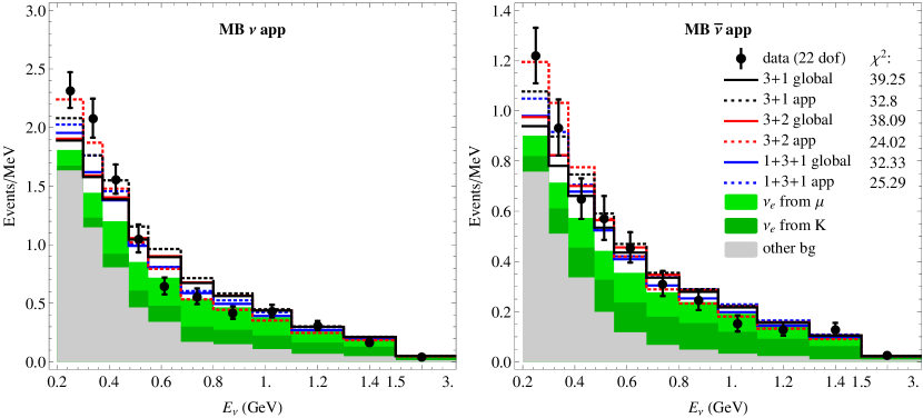
In our analysis of the MiniBooNE and appearance search we use the latest data777The recent updated analysis from MiniBooNE Aguilar-Arevalo:2013ara is based on the same data as AguilarArevalo:2012va , corresponding to protons on target in neutrino mode and protons on target in anti-neutrino mode. from AguilarArevalo:2012va , following closely the analysis instructions provided by the collaboration. Details are given in appendix E.4. Since their very first data release in 2007 AguilarArevalo:2007it , MiniBooNE observe an excess of events over expected background in the low energy ( MeV) region of the event spectrum AguilarArevalo:2008rc . Since the spectral shape of the excess is difficult to explain in a two-flavor oscillation framework, historically the analysis window has been (somewhat artificially) divided into a low energy region containing the excess events and a high energy part with no excess.888The importance of energy reconstruction effects for the low energy excess has been pointed out in Refs. Martini:2012fa ; Martini:2012uc , see also Aguilar-Arevalo:2013ara . Preliminary results from anti-neutrinos showed also some indication for an event excess in the high energy part of the spectrum AguilarArevalo:2010wv which indicated the need for CP violation in order to reconcile neutrino and anti-neutrino data. However, for the most recent data AguilarArevalo:2012va ; MBnu2012 the shapes of the neutrino and anti-neutrino spectra appear to be consistent with each other, showing excess events below around 500 MeV and data consistent with background in the high energy region, see Fig. 6. In our work we always analyse the full energy spectrum for both neutrinos and anti-neutrinos. Contrary to the analysis of the MiniBooNE collaboration we take into account oscillations of all background components in a consistent way, according to the particular oscillation framework to be tested, see appendix E.4 for details.

In Fig. 7 we show a summary of the data in the 3+1 scheme. We observe an allowed region from MiniBooNE anti-neutrino data that is driven by the event excess below around 800 MeV and has significant overlap with the parameter region preferred by LSND. At the 99% CL shown in the figure, MiniBooNE neutrino data give only an upper bound, although we find closed regions (again driven by the low-energy excess) at lower confidence levels. This is in qualitative agreement with the results obtained by the MiniBooNE collaboration, compare Fig. 4 of AguilarArevalo:2012va or Fig. 3 of Aguilar-Arevalo:2013ara . The different shape of our regions is due to the oscillations of the background components. Those can be relatively large in an appearance only fit, since for fixed we allow and to vary freely, subject to the constraint Eq. (18). We have checked that when we adopt the same assumptions as the MiniBooNE collaboration we recover their regions/bounds with good accuracy.
The recent constraint on appearance from ICARUS Antonello:2012pq at long-baseline leads to a bound on essentially independent of in the range shown here. It excludes in particular the region of large mixing and low that is otherwise unconstrained by appearance experiments.999Note that this region is also excluded by and disappearance searches once Eq. (18) is used to relate to the effective mixing angles probed by the disappearance experiments. An important background for the driven search in ICARUS are appearance events due to and . Furthermore, as discussed in section 2 and appendix A the long-baseline appearance probability in the 3+1 scheme depends on one complex phase. In deriving the ICARUS bound shown in Fig. 7 we fix the parameters and but marginalize over the relevant complex phase.
As visible in Fig. 7 there is a consistent overlap region for all experiments and we can perform a combined analysis. The resulting region is shown in red in Fig. 7. The best fit point is at , with dof (GOF = 3.7%). The no-oscillation hypothesis is excluded with respect to the best fit point with . This large value is mostly driven by LSND. The relatively low GOF comes mainly from MiniBooNE neutrino data, as can be seen from Tab. 6, where we list the individual contribution of the experiments to the total appearance . This is also obvious from Fig. 6, showing that at the 3+1 appearance best fit point (black dotted histogram) the fit to the neutrino spectrum is not very good, predicting too much excess in the region GeV and only partially explaining the excess in the data below 0.4 GeV.
| Experiment | / | dof | / | dof | / | dof |
|---|---|---|---|---|---|---|
| LSND | 11.0/ | 11 | 8.6/ | 11 | 7.5/ | 11 |
| MiniB | 19.3/ | 11 | 10.6/ | 11 | 9.1/ | 11 |
| MiniB | 10.7/ | 11 | 9.6/ | 11 | 12.7/ | 11 |
| E776 | 32.4/ | 24 | 29.2/ | 24 | 31.3/ | 24 |
| KARMEN | 9.8/ | 9 | 8.6/ | 9 | 9.0/ | 9 |
| NOMAD | 0.0/ | 1 | 0.0/ | 1 | 0.0/ | 1 |
| ICARUS | 2.0/ | 1 | 2.3/ | 1 | 1.5/ | 1 |
| Combined | 87.9/ | () | 72.7/ | () | 74.6/ | () |
Analysing the same data in the 3+2 scheme we find a best fit point at , , with (GOF = 19%). The GOF improves considerably with respect to 3+1. We find
| (19) |
For 3 dof (corresponding to the 3 additional SBL appearance parameters in 3+2) this implies that appearance data favor 3+2 over 3+1 at the 99.8% CL. From Tab. 6 we see that basically all experiments have a reasonable /dof value (maybe with the exception of E776, which intrinsically has a somewhat high ). In particular MiniBooNE neutrino data improve by 8.7 units compared to 3+1. This is also visible in Fig. 6, with the red dotted curve (3+2 appearance best fit) showing a much better fit than the black dotted one (3+1 appearance best fit), with for 22 dof for the joint MiniBooNE neutrino and anti-neutrino data. The appearance data fit in a 1+3+1 scheme is similar to the 3+2 case, with a slightly better fit for LSND and MiniBooNE neutrino, and a slightly worse fit for MiniBooNE anti-neutrino data, compare Tab. 6. The predicted MiniBooNE spectra at the 1+3+1 appearance best fit are shown as blue dotted histograms in Fig. 6. We find for 1+3+1 (GOF = 15%) and
| (20) |
6 Combined analysis of global data
We now address the question whether the hints for sterile neutrino oscillations discussed above can be reconciled with each other as well as with all existing bounds within a common sterile oscillation framework. In section 6.1 we discuss the 3+1 scenario, whereas in section 6.2 we investigate the 3+2 and 1+3+1 schemes.
6.1 3+1 global analysis

In the 3+1 scheme, SBL oscillations are described by effective 2-flavor oscillation probabilities, involving effective mixing angles for each oscillation channel. The expressions for the effective angles , , governing the disappearance, disappearance, and appearance probabilities are given in Eqs. (8), (15), (18), respectively. From those definitions it is obvious that the three relevant oscillation amplitudes are not independent, since they depend only on two independent fundamental parameters, namely and . Neglecting terms of order () one finds
| (21) |
Hence, the appearance amplitude relevant for the LSND/MiniBooNE signals is quadratically suppressed by the disappearance amplitudes, which both are constrained to be small. This leads to the well-known tension between appearance signals and disappearance data in the 3+1 scheme, see e.g. Bilenky:1996rw ; Okada:1996kw for early references.
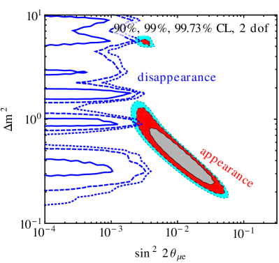
This tension is illustrated for the latest global data in the left panel of Fig. 8, where we show the allowed region for all appearance experiments (the same as the combined region from Fig. 7), compared to the limit from disappearance experiments in the plane of and . The preferred values of for disappearance data come from the reactor and Gallium anomalies. The regions for disappearance data, however, are not closed in this projection in the parameter space and include , which always can be achieved by letting because of the non-observation of any positive signal in SBL disappearance. The upper bound on from disappearance emerges essentially as the product of the upper bounds on and from and disappearance according to Eq. (21). We observe from the plot the clear tension between those data sets, with only marginal overlap regions at above 99% CL around and at 3 around .
The tension between disappearance and appearance experiments can be quantified by using the so-called parameter goodness of fit (PG) test Maltoni:2002xd ; Maltoni:2003cu . It is based on the definition
| (22) |
where is the minimum of the global data combined, and are the minima of appearance and disappearance data taken separately, and is evaluated at the best fit point of the global data. should be evaluated with the number of dof corresponding to the number of parameters in common between appearance and disappearance data (2 in the case of 3+1). From the numbers given in Tab. 7 we observe that the global 3+1 fit leads to /dof = 712/680 with a p-value 19%, whereas the PG test indicates that appearance and disappearance data are consistent with each other only with a p-value of about . The strong tension in the fit is not reflected in the global minimum, since there is a large number of data points not sensitive to the tension, which leads to the “dilution” of the GOF value in the global fit, see Maltoni:2003cu for a discussion. In contrast, the PG test is designed to test the consistency of different parts of the global data.
| /dof | GOF | /dof | PG | |||||
|---|---|---|---|---|---|---|---|---|
| 3+1 | 712/() | 19% | 18.0/2 | 95.8/68 | 7.9 | 616/621 | 10.1 | |
| 3+2 | 701/() | 23% | 25.8/4 | 92.4/68 | 19.7 | 609/621 | 6.1 | |
| 1+3+1 | 694/() | 30% | 16.8/4 | 82.4/68 | 7.8 | 611/621 | 9.0 |
The conflict between the hints for -scale oscillations and null-result data is also illustrated in the right panel of Fig. 8. In red we show the parameter regions indicated by the combined hints for oscillations including SBL reactor, Gallium, LSND, and MiniBooNE appearance data. Those regions are compared to the constraint emerging from all other data. We find no overlap region at 99% CL. Hence, an explanation of all anomalies within the 3+1 scheme is in strong tension with constraints from various null-result experiments.
| [] | [] | ||||||
|---|---|---|---|---|---|---|---|
| 3+1 | 0.93 | 0.15 | 0.17 | ||||
| 3+2 | 0.47 | 0.13 | 0.15 | 0.87 | 0.14 | 0.13 | |
| 1+3+1 | 0.15 | 0.13 | 0.47 | 0.13 | 0.17 |
6.2 3+2 and 1+3+1 global analyses
Now we move to the global analysis within a two-sterile neutrino scenario in order to investigate whether the additional freedom allows to mitigate the tension in the fit. We give and PG values for the 3+2 and 1+3+1 schemes in Tab. 7 and the corresponding values of the parameters in Tab. 8. We observe from the PG values that the tension between appearance and disappearance data remains severe, especially for the 3+2 case, with a PG value below , even less than for 3+1. For 1+3+1 consistency at the 2 per mille level can be achieved.
Let us first discuss the 3+2 fit. We find a modest improvement of the total in the global fit compared to 3+1 by
| (23) |
Evaluated for 4 additional parameters relevant for SBL data in 3+2 compared to 3+1 this corresponds to 96.9% CL.
The origin of the very low parameter goodness of fit can be understood by looking at the contributions of appearance and disappearance data to . Tab. 7 shows that the of appearance data at the global best fit point, , changes only by about 3 units between 3+1 and 3+2. However, if appearance data is fitted alone, an improvement of 15.2 units in is obtained when going from 3+1 to 3+2, see Eq. (19). The fact that appearance data by themselves are fitted much better in 3+2 than in 3+1 leads to the large value of , with a contribution of 19.7 from appearance data. In other words: the fit to appearance data at the global 3+2 best fit point (/68, p-value 2.6%) is much worse than at the appearance-only 3+2 best fit point (, p-value 19%). This interpretation is also supported by Fig. 6, showing an equally bad fit to MiniBooNE neutrino data at the 3+1 and 3+2 global best fit points (black solid and red solid histograms, respectively).

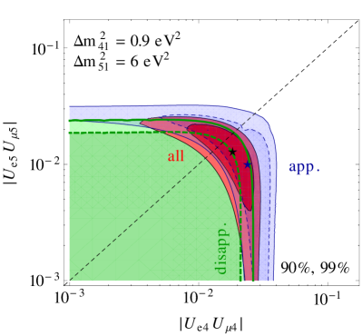
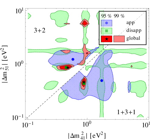
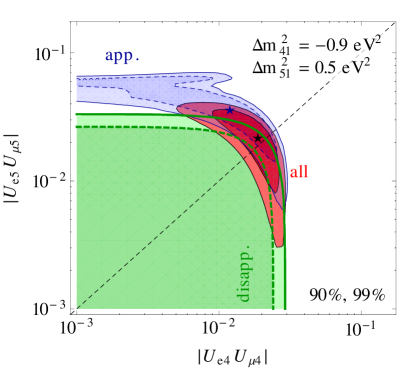
We further investigate the origin of the tension in the 3+2 fit in Figs. 9 and 10. In Fig. 9 we show the allowed regions in the multi-dimensional parameter space projected onto the plane of the two mass-squared differences for appearance and disappearance data separately, as well as the combined region. The 3+2 global best fit point happens close to an overlap region of appearance and disappearance data at 95% CL in that plot. However, an overlap in the projection does not imply that the multi-dimensional regions overlap. In the left panel of Fig. 10 we fix the mass-squared differences to values close to the global 3+2 best fit point and show allowed regions in the plane of and . These are the 5-neutrino analogs to the 4-neutrino SBL amplitude . Similar as in the 3+1 case we observe a tension between appearance and disappearance data, with no overlap at 99% CL. This explains the small PG probability at the 3+2 best fit point. The right panel of Fig. 10 corresponds to the local minimum of the combined fit visible in Fig. 9 around , . In this case no tension is visible in the mixing parameters shown in Fig. 10, however, from Fig. 9 we see that those values for the mass-squared differences are actually not preferred by appearance data, which again leads to a degraded GOF. We conclude that the tension between appearance and disappearance data cannot be resolved in the 3+2 scheme.
For the 1+3+1 ordering of 5-neutrino mass states a somewhat better fit can be obtained. We find
| (24) |
corresponding to disfavoring 3+1 at the 99.9% CL (4 dof) compared to 1+3+1. We observe from Tab. 7 that at the 1+3+1 global best fit point a much better fit to appearance data is obtained than at the 3+2 best fit point ( compared to 92.4). As visible from the blue solid histogram in Fig. 6 the lack of an event excess in the MiniBooNE neutrino spectrum around 0.6 GeV is reasonably well reproduced at the 1+3+1 global best fit point, although the low energy excess is still under-predicted. The for appearance versus disappearance for 1+3+1 is even slightly less than for 3+1 (16.8 versus 18.0). Because of the additional parameters relevant for the evaluation of the p-value 0.2% is obtained for 1+3+1, about one order of magnitude better than in 3+1.
The projection of the allowed regions on the plane of the mass-squared differences is shown in the lower-right part of Fig. 9. Note that the disappearance regions are to good accuracy symmetric for 3+2 and 1+3+1. This can be understood from Eq. (3), where the difference between 3+2 and 1+3+1 appears only in the last term, which is suppressed by the 4th power of small matrix elements, compared to the leading terms at 2nd order. We observe in Fig. 9 that appearance and disappearance regions for 1+3+1 both overlap with the combined best fit point. In Fig. 11 we show again a section through the parameter space at fixed values for the mass-squared differences close to the global best fit point. Although the tension between appearance and disappearance is still visible (no overlap of the 90% CL regions) the disagreement is clearly less severe than in the 3+2 situation shown in the left panel of Fig. 10, and in Fig. 11 we find significant overlap at 99% CL, in agreement with the somewhat improved PG p-value.
7 Summary and discussion
We have investigated in detail the status of hints for -scale neutrino oscillations, namely the indications for disappearance due to the reactor and Gallium anomalies, and the indications for appearance from LSND and MiniBooNE. Those hints have been analysed in the context of the global data on neutrino oscillations, including short and long-baseline accelerator and reactor experiments, as well as atmospheric and solar neutrinos. Our main findings can be summarized as follows.
-
1.
For all fits a global is obtained in our analysis, involving 689 data points in total, see table 7.
-
2.
However, a joint fit of all anomalies suffers from tension between appearance and disappearance data, mainly due to the strong constraints from disappearance data.
-
3.
The tension in the fit is driven by the LSND and MiniBooNE appearance hints, since oscillations in the channel inevitably predict also a signal in disappearance, which is not observed at the relevant scale.
-
4.
In contrast, the reactor and Gallium anomalies are not in direct conflict with other data, since and disappearance at the scale are controlled by independent parameters.
-
5.
In a 3+1 scheme the compatibility of appearance and disappearance data is at the level of . The individual allowed regions have marginal overlap at about 99% CL.
-
6.
We do not find a very significant improvement of the fit in a 3+2 scheme compared to 3+1. Based on the relative minima, 3+1 is disfavored with respect to 3+2 at 96.9% CL. The compatibility of appearance and disappearance data in 3+2 is even worse than in 3+1, because the fit of appearance data-only is significantly better in 3+2 than in 3+1, however, the appearance fit at the global best fit point is only marginally improved.
-
7.
We find an improvement of the global fit in the 1+3+1 spectrum compared to 3+1, at the 99.9% CL. The compatibility of appearance and disappearance data is still low in 1+3+1, at the level of 0.2%.
Hence, in all cases we find significant tension in the fit, with the marginal exception of the 1+3+1 scheme. At our 1+3+1 best fit point the minimal value for the sum of all neutrino masses would be eV, where we took the values given in Tab. 8 and assumed that the mass-squared difference with the smaller absolute value is negative, using the symmetry and of SBL data, see Eqs. (1) and (3). It remains an interesting question whether such a large value of is consistent with cosmology, see e.g. Hamann:2011ge ; Giusarma:2011ex ; GonzalezGarcia:2010un ; Joudaki:2012uk ; Archidiacono:2013xxa .
Let us briefly compare our results to two other recent global sterile neutrino fits, from Refs. Conrad:2012qt and Archidiacono:2013xxa . We are in good agreement with the results of Conrad:2012qt . For instance, in Tab. 2 of Conrad:2012qt values for the consistency of appearance and disappearance data are given, 17.8 for 3+1 and 23.9 for 3+2, which compare well with our numbers from Tab. 7, 18.0 and 25.8, respectively. There is some disagreement with the results of Archidiacono:2013xxa . The corresponding values reported in their Tab. I are 6.6 and 11.12, which lead to significantly better compatibility of appearance and disappearance data. Comparing Fig. 1 of Archidiacono:2013xxa with our Fig. 8 (left) we observe that our disappearance limits are somewhat stronger and our appearance region is at somewhat larger mixing angles, both effects increasing the tension. Our appearance region is in good agreement with Fig. 6 (left) of Conrad:2012qt . There are some differences between our disappearance region and Fig. 6 (right) of Conrad:2012qt , mainly at high .
Irrespective of the hints for disappearance and appearance, we have derived constraints on the mixing of eV-scale states with the -neutrino flavor. Those are dominated by data involving information from neutral-current interactions, which are solar neutrino data (NC matter effect and SNO NC data), MINOS long-baseline NC data, and atmospheric neutrino data (NC matter effect). The global limit is dominated by the latter.
In conclusion, establishing sterile neutrinos at the eV-scale would be a major discovery of physics beyond the Standard Model. At present a consistent interpretation of all data indicating the possible presence of eV-scale neutrino mass states remains difficult. The global fit suffers from tension between different data sets. An unambiguous solution to this problem is urgently needed. We are looking forward to future data on oscillations at the scale Abazajian:2012ys , as well as new input from cosmology.
Acknowledgments
Numerical results presented in this paper have been obtained on computing infrastructure provided by Fermi National Accelerator Laboratory and by Max Planck Institut für Kernphysik. The authors would like to thank the MINOS collaboration for their invaluable help in including their sterile neutrino search in this work. We are especially grateful to Alexandre Sousa and Mary Bishai for sharing their Monte Carlo results. We are grateful to M. Smy for providing assistance on the simulation of SK4 solar data, and to Bill Louis for valuable information on the MiniBooNE analysis. Fermilab is operated by Fermi Research Alliance under contract DE-AC02-07CH11359 with the US Department of Energy. P.A.N.M. was supported by the Fundação de Amparo à Pesquisa do Estado de São Paulo. M.M. is supported by Spanish MINECO (grants FPA-2009-08958, FPA-2009-09017, FPA2012-31880, FPA2012-34694, consolider-ingenio 2010 grant CSD-2008-0037 and “Centro de Excelencia Severo Ochoa” program SEV-2012-0249) and by Comunidad Autonoma de Madrid (HEPHACOS project S2009/ESP-1473). P.A.N.M. and M.M. acknowledge partial support from the European Union (FP7 Marie Curie-ITN actions PITN-GA-2009-237920 “UNILHC”). M.M. and T.S. acknowledge partial support from the European Union FP7 ITN INVISIBLES (Marie Curie Actions, PITN-GA-2011-289442).
Appendix A Complex phases in sterile neutrino oscillations
In this appendix we discuss in some detail the phases for neutrino oscillations involving extra sterile neutrino states. For definiteness, we will focus on ; the special case of can be easily obtained by dropping all terms containing a redundant “5” index. Let us order the flavor eigenstates as and introduce the following parametrization for the mixing matrix, with :
| (25) |
where represents a complex rotation by an angle and a phase in the plane. Note that rotations involving only sterile states (i.e., with both ) are unphysical, and therefore we have omitted them from Eq. (25). Removing those unphysical angles, contains physical angles.
In Eq. (25) we have chosen a priori all rotations to be complex. We present now a method which allows to remove unphysical phases from the mixing matrix in a consistent way. First, we note that a complex rotation can be written as
| (26) |
where is a real rotation matrix, is a diagonal matrix with for and for . Depending on whether or , the phase in is either . Second, we note that phase matrices at the very left or right of the matrix drop out of oscillation probabilities and are therefore unphysical.101010In this work we focus on neutrino oscillations. In cases where lepton-number violating processes are relevant, such as neutrino-less double beta-decay, more phases will lead to physical consequences and our phase counting does not apply. In particular, in such a case the phases on the right of the mixing matrix (these are the so-called Majorana phases) cannot be absorbed. Hence, we have to represent all matrices in Eq. (25) using Eq. (26), and then try to commute as many phase matrices to the left and the right. The matrix commutes with a matrix if and . Furthermore, if or we can commute with a complex matrix by re-defining the phase : e.g., . However, we cannot commute with a real matrix if or .
This leads to the following rule for removing phases. Let us start by removing one phase, let’s take for instance , obtaining a real . Then we can no longer use the matrices and to remove phases, since we cannot commute them with to the very left or right of . But, we can use for instance to remove one of the remaining phases , and so forth. Hence, we can remove in total phases. Starting with all physical angles complex, we obtain that there are physical phases, i.e., 1 phase for no sterile neutrinos, 3 phases for the 3+1 spectrum, and 5 phases for the 3+2 spectrum. Those remaining phases cannot be associated arbitrarily to the but only in a way which is consistent with the above prescription to remove phases. In particular, it is not possible to make simultaneously three rotation matrices , , real. One possible choice is the one given in Eq. (6). Using this recipe to remove phases it is also straightforward to obtain the physical phases in case of the SBL or LBL approximations according to Tab. 2.
In the SBL approximation for a 3+2 scheme, only two physical phases remain. In the parametrization invariant notation from Eqs. (1) and (2), they are given by and . Since the only SBL appearance experiments we consider are studying the oscillation channels only the phase is relevant for our analysis. In the specific parametrization from Table 2, the physical phases have been chosen as and . Since does not appear in the parametrization independent representation of according to Eq. (2) we can remove it from our SBL analysis without loss of generality.
In the LBL limit, more phases are phenomenologically relevant. In particular, Eq. (4) shows that the oscillation probabilities in the 3+2 case are sensitive to the parametrization independent phases
| (27) |
with defined in Eq. (2). The experiments for which the LBL approximation is relevant are ICARUS and MINOS. ICARUS searches for transitions, whereas the NC data in MINOS are sensitive to the combination . Therefore, for our analyses the two appearance channels and are relevant, leading, according to Eq. (27), to four independent phases, in agreement with Tab. 2.111111In deriving Eq. (4) we have assumed that are infinite. Note that this assumption does not reduce the number of physical phases further, since also the general procedure used in Tab. 2 (assuming only ) leads to the same number of physical phases as Eq. (4). The particular parametrization from the table implies that for the channel only the phases and are relevant, whereas the channel is also sensitive to and .
From the way we have chosen the complex rotations in Tab. 2 the correct phases in the 3+1 case are automatically obtained by dropping all rotations including the index “5” in the 3+2 mixing matrix. We recover the well-known result that in the SBL approximation in a 3+1 scenario no complex phase appears. In the LBL approximation two phases remain, corresponding to the combinations and , which can be parametrized by using the phases and , where for the channel only is relevant.
Let us comment also on the role of phases in solar and atmospheric neutrinos. As shown in appendix C solar neutrinos do depend on one effective complex phase. This is included in our analysis in full generality however the numerical impact of this phase dependence is small. It has been shown in Maltoni:2007zf (appendix C) that the impact of complex phases on atmospheric neutrinos is very small and we neglect their effect in the current analysis.
Appendix B Systematic uncertainties in the reactor analysis
The correlation of errors between SBL reactors are quite important in order to obtain the significance of the reactor anomaly. Here we describe our error prescription for the SBLR analysis. From the errors quoted in the original publications we extracted the following components. First we removed the uncertainty on the neutrino flux prediction, since we include this uncertainty in a correlated way for all reactor experiments based on the prescription given in Huber:2011wv (see below). The remaining error is divided into uncorrelated errors (including statistical as well as experimental contributions) as well as correlated errors between some SBLR measurements. The total uncorrelated error is shown in the last column of Tab. 3. Below we give details on our assumptions on correlations.
The total error on the measured cross section per fission in Bugey4 is 1.38% Declais:1994ma . It receives contributions which are reactor/site specific (1.09%) as well as detector specific (0.84%). Rovno91 Kuvshinnikov:1990ry used the same detector as Bugey4. The errors on the experimental cross section comes from the reactor and geometry (2.1%) and the latter from the detector (1.8%). So the first one should be uncorrelated whereas the second one should be correlated with the corresponding one from Bugey4. Hence we have , , , .
The Bugey3 measurement consists of 3 detectors at the distances 15 m, 40 m, 95 m. In Tab. 9 of Declais:1994su systematic errors of 5% (absolute) and 2% (relative) are quoted. The uncorrelated errors given in our Tab. 3 are obtained by adding the statistical error (Tab. 10 of Declais:1994su ) to the 2% relative systematic error. For the correlated error we remove the relative systematic error as well as 2.4% for the flux prediction and obtain , which we take fully correlated between the 3 rate measurements. In cases when we include the spectral data from Bugey3 we use 2% (3.9%) as uncorrelated (correlated) normalization errors for the three spectra. Details of our spectral analysis of Bugey3 can be found in Grimus:2001mn .
In Goesgen the same detector was used at three different distances. In Tab. V of Zacek:1986cu the individual and correlated errors are given. The values for the uncorrelated errors used in our analysis (see Tab. 3) are obtained by adding the statistical and uncorrelated systematic errors in quadrature and expressed in percentage of the ratio. Then Zacek:1986cu quotes a correlated error of 6%, which includes 3% from the neutrino spectrum, 2% from the cross section, 3.8% from efficiency, 2% from reactor power, and a few more %. We remove the 3% neutrino spectrum, as well as the 2% from cross section (this seems way too large). This gives . Part of this error is supposed to be correlated with ILL, since they used a “nearly identical” detector. Removing the reactor power of 2% we get . In the ILL paper Kwon:1981ua errors of 3.66% statistical and 11.5% systematical are quoted. The contributions to the systematic error are given as 6.5% on the “intensity of the anti-neutrino energy spectrum”, 8% detection efficiency, 1.2% neutron life time and some other smaller contributions. In the lack of detailed information we proceed as follows. We remove 3% for the flux uncertainties (the same as in Goesgen) and take 8% (the detection efficiency) to be correlated with Goesgen. This gives and , where the uncorrelated error includes also the statistical one. We have checked that other “reasonable” assumptions on the ILL/Goesgen correlation do not change our results significantly.
From Krasnoyarsk Vidyakin:1987ue ; Vidyakin:1994ut there are three data points based on a single detector, which records events from 2 “identical” reactors. In Vidyakin:1987ue from 1987, results at distances of 32.8 m and 92.3 m are reported. The statistical errors are 3.55% and 19.8%, respectively, and the systematical error are 4.84% and 4.76%, respectively, which include detector effects (), reactor power () and the effective distance (). We take systematical errors fully correlated between those two data points. Then there is a measurement from 1994 Vidyakin:1994ut at 57 m. The errors include detector uncertainty (3.4%), reactor power (2.5%), and statistics (0.95%). We assume the detector error to be correlated with the 1987 data points but include the reactor power in the uncorrelated error.
For SRP Greenwood:1996pb measurements at the distances of 18 m and 24 m are reported from the same detector, which has been moved between the two positions. The obtained ratios of data over expectation at the two distances are and . The uncorrelated systematic error is derived from the ratio of the two spectra, , with an expectation of 1.73 Greenwood:1996pb . Hence is an uncorrelated systematic error. Then we remove the 2.5% from the neutrino spectrum from the systematical error and obtain , , and . With this assumption on the uncorrelated errors the two data points are consistent at about .
Rovno88 Afonin:1988gx reports 5 measurements with two different detectors: 1I, 2I, 1S, 2S, 3S, where the “I” experiments use an integral neutron detector, whereas the “S” experiments use a scintillation detector measuring the positron spectrum. In Tab. III of Afonin:1988gx for each measurement two systematical errors are given, 2.2% for “the uncertainty in the measured reactor power and the geometric uncertainty”, and a second uncertainty due to “errors in the detector characteristics and fluctuations”. From Tab. II one finds that statistical errors are negligible. In the absence of detailed information we assume the 2.2% uncertainty fully correlated among all experiments. From the second error we assume that half of it is uncorrelated and the other half is correlated among detectors of the same type. We have checked that our results do not depend significantly on those assumptions.
Finally let us comment on the uncertainty on the neutrino flux predictions. As mentioned above this uncertainty has been removed from the SBLR experimental errors since they are treated in a correlated way for all reactor experiments. For the uncertainties of the fluxes from 235U, 239Pu, 241Pu we use the information from tables provided in Huber:2011wv . The uncertainty is provided as uncorrelated error in each bin of neutrino energy as well as fully correlated (between energy bins as well as the three isotopes) errors. For the uncorrelated errors we proceed as follows. We perform a fit of a polynomial of 2nd order to the numbers given in Huber:2011wv . Then those coefficients are used as pulls in the analysis constrained by the covariance matrix obtained from the polynomial fits. This allows us to take into account the fact that the bin-to-bin uncorrelated errors of the neutrino spectrum will lead to correlated effects in the observed positron spectra. Since the uncorrelated flux errors are sub-leading compared to the correlated ones the parametrization with a 2nd order polynomial is sufficiently accurate. To include the correlated errors we follow Huber:2011wv : the various contributions to this error in each neutrino energy bin are symmetrized and added in quadrature. Then we obtain an energy dependent fully correlated error for the spectra from 235U, 239Pu, 241Pu which is included as one common pull parameter in the global reactor . For the neutrinos from 238U we use the flux from Mueller:2011nm and include a global normalization error on the 238U induced events of 8.15% Mention:2011rk .
Appendix C Solar neutrino analysis
In the analysis of solar neutrino experiments we include the total rates from the radio chemical experiments Chlorine Cleveland:1998nv , GALLEX/GNO Kaether:2010ag and SAGE Abdurashitov:2009tn . Regarding real-time experiments, we include the electron scattering energy-zenith angle spectrum data from all the Super-Kamiokande phases I–IV Hosaka:2005um ; Cravens:2008aa ; Abe:2010hy ; SKnu2012 and the data from the three phases of SNO Aharmim:2007nv ; Aharmim:2005gt ; Aharmim:2008kc . We also include the main set of the 740.7 days of Borexino data Bellini:2011rx as well as their high-energy spectrum from 246 live days Bellini:2008mr . In total the solar neutrino data used in our analysis consists of 261 data points.
Let us now focus on the probabilities relevant for the analysis of solar neutrino experiments. We will assume that only the first two mass eigenstates are dynamical, while the others are taken to be infinite. Since physical quantities have to be independent of the parameterization of the mixing matrix, we will use the freedom in choosing a parameterization that makes analytical expressions particularly simple. We start from the Hamiltonian in the flavor basis:
| (28) |
where and . It is convenient to write , where is a complex rotation by an angle and a phase which we will define later.121212We define in such a way that the corresponding rotation is the rightmost rotation in , but we do not assume anything about all other rotations. If the standard parameterization is used for them, then has the usual interpretation. Then we can write:
| (29) |
In order to further simplify the analysis, let us now assume that all the mass-squared differences involving the “heavy” states with can be considered as infinite: and for any and . In leading order, the matrix takes the effective block-diagonal form:
| (30) |
where is the sub-matrix of corresponding to the first and second neutrino states, and is a diagonal matrix (the matter terms in this block are negligible in the limit of very large ). Consequently, the evolution matrix is:
| (31) |
We are interested only in the elements . It is convenient to define in such a way that . Taking into account the block-diagonal form of , we obtain:
| (32) |
The expressions for the probabilities, , are straightforward:
| (33) |
Here we have used the fact that the terms containing a factor oscillate very fast, and therefore vanish once the finite energy resolution of the detector is taken into account. For solar neutrino experiments we only need and . It is therefore convenient to define in such a way that is a real number. Let us also define:
| (34) |
Using unitarity relations, and , we obtain:
| (35) |
where
| (36) |
In the above expressions and are effective terms derived from the Hamiltonian , which has the form:
| (37) |
with the vacuum term including the phase :
| (38) |
These equations are valid for any number of extra sterile states. Hence, in the most general case solar neutrinos depend on six real mixing parameters,
| (39) |
one complex phase (), and . Let us now further define and discuss some special limits:
-
•
: this implies , hence for . By unitarity , hence for . Therefore, and ; the probabilities reduce to the well-known expressions and with ;
-
•
: in this case , sterile neutrinos do not participate to 1-2 oscillations and is a constant. If we further assume that no sterile neutrino exists then and , so that and reduces to the well-known three-neutrino formula;
-
•
: for one sterile neutrino reduces to .
To perform the analysis we map the parameters which are used for the analysis into the effective parameters for solar neutrinos. In the case of 3+1 the number of real mixing parameters is actually the same as the number of mixing angles in the most general parametrization of the mixing matrix: the six parameters in Eq. (39) are a function of the six angles , , , , , . The dependence of solar neutrinos on is shown in Fig. 3 and the one on follows from Fig. 5. The dependence on is important for the NC matter effect and SNO NC data. For the number of effective mixing parameters of solar data is less than the number of angles in the general mixing matrix. The phase is a complicated function of complex phases and angles. We have verified numerically for the 3+1 case that if all angles are non-zero (and relatively large) the from solar data varies by about 1 to 2 units as a function of the phase. Once all relevant constraints on the mixing angles are imposed the effect of the phase on solar data is negligible. See also Long:2013hwa for a discussion of complex phases in solar neutrinos in the context of sterile neutrinos.
Appendix D Atmospheric neutrino analysis
The analysis of atmospheric data follows closely the one presented in Refs. GonzalezGarcia:2010er ; GonzalezGarcia:2011my and includes the Super-Kamiokande results from phases I, II and III Wendell:2010md (80 data points in total). Technical details on our fit can be found in the appendix of GonzalezGarcia:2007ib .
In order to derive suitable expressions for the relevant probabilities, we can follow the approach presented in App. C for solar data. The Hamiltonian in the flavor basis is given by Eq. (28), which in the mass basis becomes:
| (40) |
As before, we can simplify the analysis by assuming that all the mass-squared differences involving the “heavy” states with can be considered as infinite: and for any and . In leading order, the matrix takes the effective block-diagonal form:
| (41) |
where is the sub-matrix of corresponding to the first, second and third neutrino states, and is a diagonal matrix (the matter terms in this block are negligible in the limit of very large ). We are interested only in the probabilities with . Taking into account the block-diagonal form of , we obtain:
| (42) |
where and is the sub-matrix corresponding to the first three lines and columns of , and as such it is not a unitary matrix.
Let us now focus on the three-neutrino system described by , with . The matter term contains both the “standard” contribution from charged-current interactions, and a “non-standard” part induced by the absence of neutral-current interactions for sterile neutrinos. In practical terms, this is just the same as the problem of neutrino propagation in the presence of non-standard neutrino-matter interactions (NSI) described in Ref. GonzalezGarcia:2011my . Following the approach discussed there, we make a number of simplifying assumptions:
-
•
we assume that the neutron-to-electron density ratio, , is constant all over the Earth. We set as inferred from the PREM model Dziewonski:1981xy ;
-
•
we set , thus forcing the vacuum term to have two degenerate eigenvalues;
-
•
we impose that the matter term also has two degenerate eigenvalues.
The first two assumptions are very well known hand have been discussed in detail in the literature. For example, in Sec. 5.2 of Ref. GonzalezGarcia:2007ib it was noted that the different chemical composition of the Earth mantle and core has very little impact on NSI results. The last approximation is adopted here for purely practical reasons, since (together with the other two) it allows to greatly simplify the calculation of the neutrino evolution Blennow:2008eb ; GonzalezGarcia:2011my . Unfortunately, in the present context the matter term cannot be fixed a priori, but it arises as an effective quantity determined by the angles and phases of the mixing matrix . Finding the points in the general parameter space for which has two degenerate eigenvalues (the only points for which our numerical analysis is technically feasible) is not an easy task. To solve this problem, we have considered here two alternative cases, both based on physically motivated scenarios:
-
(a)
decouple the electron flavor from the evolution and include the NC matter effect;
-
(b)
allow the electron flavor to participate in oscillations but neglect the NC matter effect.
Option (a) requires to set for (in addition to ), whereas option (b) is equivalent to setting (“hydrogen-Earth” model). Both approximations have been previously discussed in App. C of Ref. Maltoni:2007zf . Although we know that none of these options corresponds to Nature, we can make a sensible choice of when it is safe to use each of them. It turns out that for constraining the mixing of the with eV-scale neutrinos the NC matter effect plays no role at all (see discussion in App. C2 of Maltoni:2007zf ), whereas the participation of the electron flavor may have some impact.131313The reason is that the main information comes from effects on the overall normalization of -like events, and in order to fix this normalization the -like sample plays a role in constraining uncertainties in the neutrino fluxes. Therefore, whenever we are mainly interested in constraining (), as in the case of the global analysis combined with SBL data, we adopt assumption (b). This is important since non-zero leads to slightly relaxed constraints on , although the effect is small once external constraints on are taken into account. With respect to our former analysis presented in Ref. Maltoni:2007zf , the explicit NSI formalism adopted here is more general since it allows to fully include -related effects without further approximations.
On the other hand, when exploring the sensitivity to the fraction of sterile neutrinos participating in atmospheric and long-baseline neutrino oscillations, the contribution of neutral-current neutrino-matter interactions is essential. Indeed, under approximation (b) no limit on () would be obtained. Therefore, when exploring constraints on we adopt assumption (a) above. This is relevant for Figs. 4 (right) and 5.
Appendix E Technical details on the simulation of SBL and LBL experiments
Here we provide technical details on the simulation of some of the experiments included in our fit. All the simulations described in this appendix make use of the GLoBES software package Huber:2004ka ; Huber:2007ji .
E.1 KARMEN/LSND 12C disappearance analysis
Both LSND and KARMEN have measured the reaction , where the 12N decays back to with a lifetime of 15.9 ms. By detecting the electron from the first reaction, which has a -value of 17.33 MeV, one can infer the neutrino energy. Here we describe how we use these data to constrain disappearance Reichenbacher:2005nc ; Conrad:2011ce .
For KARMEN, we use the information from the thesis Reichenbacher:2005nc , which uses more exposure than the original publication Armbruster:1998uk . The number of expected events can be calculated by multiplying the 12C cross section (Fukugita et al. Fukugita:1988hg : ), the number of target nuclei (), the absolute neutrino flux (), the efficiency (27.2%, flat in energy), and the inverse effective scaled area (). 846 neutrino candidates are observed, with an expected background of , which are mainly accidentals and cosmic induced. The systematic errors are dominated by a 6.7% uncertainty in the absolute neutrino flux and 3% in the Monte Carlo efficiency. The total systematic error is 7.5% plus a 12% cross section error. We take the latter to be correlated between the KARMEN and LSND -carbon analyses. In fig. 3.2 (upper panel) of Reichenbacher:2005nc , the data are shown as the energy distribution of the prompt spectrum in 26 bins where the visible prompt electron energy is within the range . Modulo energy reconstruction the neutrino and electron energies would be related by the -value as . For the simulation we assume . To properly fit the data, we assume for the energy resolution. With the 26 data points we obtain a two-neutrino best fit with .
For LSND Auerbach:2001hz we compute the expected number of events by multiplying the 12C cross section ( Fukugita:1988hg ), the number of target nuclei (), the neutrino flux at the detector (), and the efficiency (23.2%, flat in energy). 733 neutrino candidates are observed, with a negligible expected background. The systematic error is dominated by a 7% uncertainty in the neutrino flux and a 6% uncertainty in the effective fiducial volume. The total systematic error, not including the theoretical cross section error, is 9.9%. The 12% cross section error is correlated between the LSND and KARMEN - analyses. In fig. 6 of Ref. Auerbach:2001hz , the data are shown as the energy distribution of the prompt spectrum, where the visible prompt electron energy is within the range and divided into 12 bins of width 2 MeV. In terms of the neutrino energy , this energy range corresponds to . In our analysis, we combine the 12 energy bins into only 6 bins. To properly fit the data, we assume MeV for the energy resolution. With the 6 data points we obtain a two-neutrino best fit with .
For the combined KARMEN+LSND -carbon fit, we have 32 bins and we find a two-neutrino best fit point with .
E.2 E776
The pion beam experiment E776 at Brookhaven Borodovsky:1992pn employed a 230 ton calorimeter detector located at approximately 1 km from the end of the 50 m long pion decay pipe. The energy of order GeV was measured with an energy resolution of 20%/. E776 used disappearance data to obtain the overall normalization of the neutrino flux. In our fit, we do not explicitly include data, but instead use the normalization as an input. The main backgrounds in E776 came from intrinsic contamination in the beam and from ’s produced in neutral current interactions and misidentified as electrons. The systematic errors were 11% for the intrinsic background and 27% (39%) for the background in neutrino (anti-neutrino) mode. In 1986, E776 collected () protons on target, and a total of 136 (56) () candidate events were observed with an expected background of 131 (62) events for neutrino (anti-neutrino) mode. E776 present the observed and predicted electron energy spectra using 14 equidistant energy bins per polarity, covering the energy range from 0 GeV to 7 GeV. In our fit we omit the first bin and combine the second and third ones because modeling the detection efficiency at these low energies is very difficult. Hence, we have a total of 24 data points. We checked that we are able to reproduce well the exclusion curve shown in fig. 4 of ref. Borodovsky:1992pn (if we also use a two-flavor oscillation model), and we obtain at the best fit point. In the combined analysis with other experiments we take into account oscillations for the background.
E.3 ICARUS
The ICARUS experiment Rubbia:2011ft is a neutrino beam experiment at Gran Sasso. The CNGS facility at CERN shoots 400 GeV protons at a graphite or beryllium target, producing a hadronic shower which is focused by a magnetic horn system. The resulting neutrino beam is mainly composed of , having only a 2% contamination and a % intrinsic component. The neutrino spectrum ranges approximately from GeV, with a wide peak at GeV. After traveling 732 km, they are detected in the ICARUS T600 detector, a 760 ton liquid argon time projection chamber. Between 2010 and 2012, the ICARUS detector observed 839 neutrino events with energy below 30 GeV, to be compared with the expectation of 627 and 3 charged current events, as well as 204 neutral current events. While a Monte Carlo simulation of the experiment predicts 3.7 background events, only two were identified Antonello:2012pq . For our ICARUS simulation, we took the spectrum from Ref. Bonesini:2006ik and folded it with the oscillation probability. To assess the limit on appearance, we define the likelihood , where () is the total observed (expected) number of events. Although there is a % systematic error in the selection efficiency, we have checked that its impact on the experiment sensitivity is negligible.
E.4 MiniBooNE
To analyze MiniBooNE data on oscillations, we use the data presented in AguilarArevalo:2012va , corresponding to protons on target in neutrino mode and protons on target in anti-neutrino mode, the same exposure as used in Aguilar-Arevalo:2013ara . We follow the analysis strategy outlined in the supporting on-line documentation AguilarArevalo:2012va . For each set of oscillation parameters we consider, we compute the expected neutrino and anti-neutrino energy spectra by weighting the unoscillated Monte Carlo events from MiniBooNE’s data release AguilarArevalo:2012va with the oscillation probabilities. For each simulated event, we take into account the individual neutrino energy and the distance between the neutrino production and detection vertices. We allow both signal and background neutrinos to oscillate including the “wrong-sign contamination” of the signal. In computing the log-likelihood for any given parameter point, we take into account statistical and systematic uncertainties by using the covariance matrix published by MiniBooNE AguilarArevalo:2012va . The likelihood is given by
| (43) |
where () is a column vector containing the observed (predicted) number of events including background, and is the covariance matrix (see Ref. AguilarArevalo:2012va for details). Note that this covariance matrix includes correlations between the and event samples as well as between neutrino and anti-neutrino data (if analysed together). There are 11 bins for -like data and 8 bins for -like data, for neutrino and anti-neutrino mode, each.
The -data are used to determine the normalization of the beam flux. In principle, we should therefore include also oscillations in the disappearance sample. The impact of oscillation on the fit to the data would then be taken into account by the covariance matrix. This is problematic because it would prevent us from combining, without double-counting, our results with the independently obtained ones from MiniBooNE’s dedicated disappearance searches (see below). Using the data from AguilarArevalo:2012va directly for a disappearance analysis is also not possible because the corresponding prediction from AguilarArevalo:2012va has been obtained from a Monte Carlo simulation in which some parameters have been tuned to the data assuming no disappearance. We have therefore decided to follow the MiniBooNE collaboration and not to include oscillations of in the appearance analysis. We have verified numerically that this has a negligible impact on the fit results once external limits on , are taken into account.
A further subtlety arises for the kaon-induced backgrounds. In MiniBooNE, these are predicted using information from the SciBooNE detector Cheng:2011wq , which operated in the same beam, but at a shorter baseline. To account for this, we rescale the kaon-induced backgrounds in MiniBooNE by the ratio of the oscillation probabilities in MiniBooNE and in SciBooNE. Since kaon-induced backgrounds make only a small contribution to MiniBooNE’s total error budget, the effect of this rescaling on the fit results is, however, very small.
Due to the correlation with the muon-like events it is not straight forward to assign a number of degrees of freedom to the appearance search without double counting the muon data, which are used also in the separate disappearance analysis. We have adopted the following prescription. Eq. (43) can be written as
| (44) |
where () are the () components of the vector , , and denotes the corresponding sub-blocks of the matrix . In Eq. (44) we have defined
| (45) |
where is the inverse of the sub-block of .141414Note that is different from , the latter being the sub-block of the inverse of . Hence, we have block-diagonalized the covariance matrix. The shift corresponds to the impact of the -like data on the normalization of the -like flux. The two terms in Eq. (44) should be statistically independent and approximately distributed. For the MiniBooNE appearance analysis we therefore use , and assign 22 dof to it (for combined neutrino/anti-neutrino data). The last equality in Eq. (45) shows explicitly that does not depend on oscillation parameters, since we neglect the effect of oscillations on . With this method we obtain GOF values which are in reasonable agreement with the numbers obtained by the collaboration: our results for dof (GOF) for neutrino, anti-neutrino, combined data are 14.2/9 (11%), 6.5/9 (69%), 32.9/20 (3.5%), respectively, compared to the numbers obtained in AguilarArevalo:2012va 13.2/6.8 (6.1%), 4.8/6.9 (67.5%), 24.7/15.6 (6.7%). Note that in AguilarArevalo:2012va the number of dof and GOF have been determined by explicit Monte Carlo study and also a different energy range has been used to obtain those numbers.
For our MiniBooNE disappearance analysis, we use the neutrino mode data from AguilarArevalo:2009yj . As in appearance mode, we compute the expected event spectra for each parameter point by using MiniBooNE’s Monte Carlo events. Since backgrounds are very small for this analysis, we do not need to take them into account. For each set of oscillation parameters, we choose the overall normalization of the spectrum in such a way that the total predicted number of events matches the number of observed events in MiniBooNE, i.e., we fit only the event spectrum, not the normalization. The log-likelihood is obtained in analogy to Eq. (43) and thus takes into account systematic uncertainties and correlations between different energy bins.
In the analysis of disappearance data, we follow the combined MiniBooNE/SciBooNE analysis from Cheng:2012yy . As for the appearance and disappearance analyses, we use public Monte Carlo data to compute the predicted event spectra. We take into account oscillations of both the signal and the background, and we compute the log-likelihood again in analogy to Eq. (43).
E.5 MINOS
Our analysis of MINOS neutral current (NC) and charged current (CC) interaction is based on protons on target of NC data presented by the collaboration in Ref. Vahle:2010 (see also Adamson:2010wi ; Adamson:2011ku ) and protons on target of CC data published in Adamson:2011ig . All data was recorded in neutrino mode, i.e., the beam consists mostly of and only small contaminations of , and .
We have implemented the properties of the NuMI beam and the MINOS detector within the GLoBES framework Huber:2004ka ; Huber:2007ji , using results from the full MINOS Monte Carlo simulations as input wherever possible. In particular, we use tabulated Monte Carlo events Sousa:privcom to construct the detector response functions and for neutral current events in the near detector (ND) and the far detector (FD), respectively. and describe the probability for a neutrino with true energy to yield an event with reconstructed energy . We include the CC and CC backgrounds to the NC event sample (beam intrinsic as well as oscillation induced), as well as the small NC background to the CC event sample. The number of charged current interactions is predicted using the simulated NuMI flux Bishai:privcom , the cross sections calculated in Messier:1999kj ; Paschos:2001np ; Andreopoulos:2009rq , and a Gaussian energy resolution function with width for the CC event sample and for the CC background in the NC event sample. The parameters of the energy resolution function, as well as the efficiencies, have been tuned in order to optimally reproduce the unoscillated event rates predicted by the MINOS Monte Carlo. We emulate the baseline uncertainty due to the non-vanishing length of the MINOS decay pipe by smearing the oscillation probabilities with an additional Gaussian of width and setting the effective distance between near detector and neutrino source to 700 m. This value as well as the parameters of the smearing function have been obtained numerically from the requirement that 2-flavor oscillation probabilities at the near detector computed with a more accurate treatment of the decay pipe are well reproduced for various mass squared differences of order eV.
We compute neutrino oscillations in MINOS numerically using a full 4- or 5-flavor code that includes all relevant mixing parameters as well as CC and NC matter effects. In the fit, we predict the expected number of events at the far detector for a given set of oscillation parameters by multiplying the observed number of near detector events in each energy bin with the simulated ratio of far and near detector events in that bin. Each event sample is divided into 20 energy bins with a width of 1 GeV each, covering the energy range from 0 to 20 GeV. As systematic uncertainties, we include in the analysis of the NC (CC) sample a 4% (10%) overall normalization uncertainty on the far-to-near ratio, separate 15% (20%) uncertainties in the background normalization at the far and near detectors, a 3% (5%) error on the energy calibration for signal events and a 1% (5%) error on the energy calibration for background events. For the NC analysis, the systematic uncertainties are based on the information given in Adamson:2010wi , for the CC analysis they have been tuned in order to reproduce the collaboration’s fit with reasonable accuracy, while still remaining very conservative.
References
- (1) Super-Kamiokande Collaboration, Y. Fukuda et al., Evidence for oscillation of atmospheric neutrinos, Phys. Rev. Lett. 81 (1998) 1562–1567, [hep-ex/9807003].
- (2) SNO Collaboration, Q. R. Ahmad et al., Direct evidence for neutrino flavor transformation from neutral-current interactions in the sudbury neutrino observatory, Phys. Rev. Lett. 89 (2002) 011301, [http://arXiv.org/abs/nucl-ex/0204008].
- (3) KamLAND Collaboration, T. Araki et al., Measurement of neutrino oscillation with kamland: Evidence of spectral distortion, Phys. Rev. Lett. 94 (2005) 081801, [hep-ex/0406035].
- (4) MINOS Collaboration, P. Adamson et al., Measurement of Neutrino Oscillations with the MINOS Detectors in the NuMI Beam, Phys. Rev. Lett. 101 (2008) 131802, [arXiv:0806.2237].
- (5) T2K Collaboration, K. Abe et al., Indication of Electron Neutrino Appearance from an Accelerator-produced Off-axis Muon Neutrino Beam, Phys.Rev.Lett. 107 (2011) 041801, [arXiv:1106.2822].
- (6) MINOS Collaboration, P. Adamson et al., Improved search for muon-neutrino to electron-neutrino oscillations in MINOS, Phys.Rev.Lett. 107 (2011) 181802, [arXiv:1108.0015].
- (7) DOUBLE-CHOOZ Collaboration, Y. Abe et al., Indication for the disappearance of reactor electron antineutrinos in the Double Chooz experiment, Phys.Rev.Lett. 108 (2012) 131801, [arXiv:1112.6353].
- (8) DAYA-BAY Collaboration, F. An et al., Observation of electron-antineutrino disappearance at Daya Bay, Phys.Rev.Lett. 108 (2012) 171803, [arXiv:1203.1669].
- (9) RENO Collaboration, J. Ahn et al., Observation of Reactor Electron Antineutrino Disappearance in the RENO Experiment, Phys.Rev.Lett. 108 (2012) 191802, [arXiv:1204.0626].
- (10) Double Chooz Collaboration, Y. Abe et al., Reactor electron antineutrino disappearance in the Double Chooz experiment, Phys.Rev. D86 (2012) 052008, [arXiv:1207.6632].
- (11) M. Gonzalez-Garcia, M. Maltoni, J. Salvado, and T. Schwetz, Global fit to three neutrino mixing: critical look at present precision, JHEP 1212 (2012) 123, [arXiv:1209.3023].
- (12) LSND Collaboration, A. Aguilar et al., Evidence for neutrino oscillations from the observation of appearance in a beam, Phys. Rev. D64 (2001) 112007, [hep-ex/0104049].
- (13) MiniBooNE Collaboration, A. Aguilar-Arevalo et al., A Search for electron neutrino appearance at the eV2 scale, Phys.Rev.Lett. 98 (2007) 231801, [arXiv:0704.1500].
- (14) MiniBooNE Collaboration, A. A. Aguilar-Arevalo et al., Event Excess in the MiniBooNE Search for Oscillations, Phys. Rev. Lett. 105 (2010) 181801, [arXiv:1007.1150].
- (15) C. Polly, “Results from MiniBooNE.” Talk at Neutrino2012, 3–9 June 2012, Kyoto, Japan, 2012.
- (16) MiniBooNE Collaboration, A. Aguilar-Arevalo et al., A Combined and Oscillation Analysis of the MiniBooNE Excesses, arXiv:1207.4809. Data and analysis instructions available at http://www-boone.fnal.gov/for_physicists/data_release/nue_nuebar_2012/combined.html#fit200.
- (17) The MiniBooNE Collaboration Collaboration, A. Aguilar-Arevalo et al., Indication of Electron Antineutrino Appearance at the Scale, arXiv:1303.2588.
- (18) M. A. Acero, C. Giunti, and M. Laveder, Limits on and disappearance from Gallium and reactor experiments, Phys.Rev. D78 (2008) 073009, [arXiv:0711.4222].
- (19) C. Giunti and M. Laveder, Statistical Significance of the Gallium Anomaly, Phys.Rev. C83 (2011) 065504, [arXiv:1006.3244].
- (20) T. A. Mueller et al., Improved Predictions of Reactor Antineutrino Spectra, Phys. Rev. C83 (2011) 054615, [arXiv:1101.2663].
- (21) P. Huber, On the determination of anti-neutrino spectra from nuclear reactors, Phys. Rev. C84 (2011) 024617, [arXiv:1106.0687].
- (22) K. Schreckenbach, G. Colvin, W. Gelletly, and F. Von Feilitzsch, Determination of the anti-neutrino spectrum from U235 thermal neutron fission products up to 9.5 MeV, Phys.Lett. B160 (1985) 325–330.
- (23) A. Hahn, K. Schreckenbach, G. Colvin, B. Krusche, W. Gelletly, et al., Anti-neutrino spectra from Pu241 and Pu239 thermal neutron fission products, Phys.Lett. B218 (1989) 365–368.
- (24) F. Von Feilitzsch, A. Hahn, and K. Schreckenbach, Experimental beta spectra from Pu239 and U235 thermal neutron fission products and their correlated anti-neutrino spectra, Phys.Lett. B118 (1982) 162–166.
- (25) P. Vogel, G. Schenter, F. Mann, and R. Schenter, Reactor anti-neutrino spectra and their application to anti-neutrino induced reactions. 2., Phys.Rev. C24 (1981) 1543–1553.
- (26) G. Mention et al., The Reactor Antineutrino Anomaly, Phys. Rev. D83 (2011) 073006, [arXiv:1101.2755].
- (27) J. J. Gomez-Cadenas and M. C. Gonzalez-Garcia, Future tau-neutrino oscillation experiments and present data, Z. Phys. C71 (1996) 443–454, [hep-ph/9504246].
- (28) S. Goswami, Accelerator, reactor, solar and atmospheric neutrino oscillation: Beyond three generations, Phys. Rev. D55 (1997) 2931–2949, [hep-ph/9507212].
- (29) S. M. Bilenky, C. Giunti, and W. Grimus, Neutrino mass spectrum from the results of neutrino oscillation experiments, Eur.Phys.J. C1 (1998) 247–253, [hep-ph/9607372].
- (30) N. Okada and O. Yasuda, A Sterile neutrino scenario constrained by experiments and cosmology, Int.J.Mod.Phys. A12 (1997) 3669–3694, [hep-ph/9606411].
- (31) O. L. G. Peres and A. Y. Smirnov, (3+1) spectrum of neutrino masses: A chance for LSND?, Nucl. Phys. B599 (2001) 3, [hep-ph/0011054].
- (32) M. Sorel, J. M. Conrad, and M. Shaevitz, A combined analysis of short-baseline neutrino experiments in the (3+1) and (3+2) sterile neutrino oscillation hypotheses, Phys. Rev. D70 (2004) 073004, [hep-ph/0305255].
- (33) M. Maltoni and T. Schwetz, Sterile neutrino oscillations after first MiniBooNE results, Phys. Rev. D76 (2007) 093005, [arXiv:0705.0107].
- (34) J. Conrad, C. Ignarra, G. Karagiorgi, M. Shaevitz, and J. Spitz, Sterile Neutrino Fits to Short Baseline Neutrino Oscillation Measurements, arXiv:1207.4765.
- (35) M. Maltoni, T. Schwetz, M. Tortola, and J. Valle, Ruling out four neutrino oscillation interpretations of the LSND anomaly?, Nucl.Phys. B643 (2002) 321–338, [hep-ph/0207157].
- (36) A. Strumia, Interpreting the LSND anomaly: sterile neutrinos or CPT- violation or…?, Phys. Lett. B539 (2002) 91–101, [hep-ph/0201134].
- (37) M. Cirelli, G. Marandella, A. Strumia, and F. Vissani, Probing oscillations into sterile neutrinos with cosmology, astrophysics and experiments, Nucl.Phys. B708 (2005) 215–267, [hep-ph/0403158].
- (38) K. Abazajian, M. Acero, S. Agarwalla, A. Aguilar-Arevalo, C. Albright, et al., Light Sterile Neutrinos: A White Paper, arXiv:1204.5379.
- (39) J. Kopp, M. Maltoni, and T. Schwetz, Are there sterile neutrinos at the eV scale?, Phys.Rev.Lett. 107 (2011) 091801, [arXiv:1103.4570].
- (40) L. Borodovsky, C. Chi, Y. Ho, N. Kondakis, W.-Y. Lee, et al., Search for muon-neutrino oscillations in a wide-band neutrino beam, Phys.Rev.Lett. 68 (1992) 274–277.
- (41) M. Antonello, B. Baibussinov, P. Benetti, E. Calligarich, N. Canci, et al., Experimental search for the LSND anomaly with the ICARUS LAr TPC detector in the CNGS beam, arXiv:1209.0122.
- (42) MINOS Collaboration, P. Adamson et al., Search for sterile neutrino mixing in the MINOS long baseline experiment, Phys.Rev. D81 (2010) 052004, [arXiv:1001.0336].
- (43) MINOS Collaboration, P. Adamson et al., Active to sterile neutrino mixing limits from neutral-current interactions in MINOS, Phys.Rev.Lett. 107 (2011) 011802, [arXiv:1104.3922].
- (44) MiniBooNE Collaboration, A. A. Aguilar-Arevalo et al., A search for muon neutrino and antineutrino disappearance in MiniBooNE, Phys. Rev. Lett. 103 (2009) 061802, [arXiv:0903.2465]. Data and analysis instructions available at http://www-boone.fnal.gov/for_physicists/data_release/numu_numubar/.
- (45) MiniBooNE Collaboration, SciBooNE Collaboration, G. Cheng et al., Dual baseline search for muon antineutrino disappearance at , arXiv:1208.0322. Data and analysis instructions available at http://www-sciboone.fnal.gov/data_release/joint_numubar_disap/.
- (46) C. Giunti and M. Laveder, Status of 3+1 Neutrino Mixing, Phys.Rev. D84 (2011) 093006, [arXiv:1109.4033].
- (47) M. Archidiacono, N. Fornengo, C. Giunti, S. Hannestad, and A. Melchiorri, Sterile Neutrinos: Cosmology vs Short-BaseLine Experiments, arXiv:1302.6720.
- (48) Y. Li and S.-s. Liu, Vanishing effective mass of the neutrinoless double beta decay including light sterile neutrinos, Phys.Lett. B706 (2012) 406–411, [arXiv:1110.5795].
- (49) J. Barry, W. Rodejohann, and H. Zhang, Light Sterile Neutrinos: Models and Phenomenology, JHEP 1107 (2011) 091, [arXiv:1105.3911].
- (50) C. Giunti and M. Laveder, Implications of 3+1 Short-Baseline Neutrino Oscillations, Phys.Lett. B706 (2011) 200–207, [arXiv:1111.1069].
- (51) J. Hamann et al., Cosmology seeking friendship with sterile neutrinos, Phys. Rev. Lett. 105 (2010) 181301, [arXiv:1006.5276].
- (52) E. Giusarma, M. Corsi, M. Archidiacono, R. de Putter, A. Melchiorri, et al., Constraints on massive sterile neutrino species from current and future cosmological data, Phys.Rev. D83 (2011) 115023, [arXiv:1102.4774].
- (53) M. C. Gonzalez-Garcia, M. Maltoni, and J. Salvado, Robust Cosmological Bounds on Neutrinos and their Combination with Oscillation Results, JHEP 08 (2010) 117, [arXiv:1006.3795].
- (54) M. Archidiacono, N. Fornengo, C. Giunti, and A. Melchiorri, Testing 3+1 and 3+2 neutrino mass models with cosmology and short baseline experiments, arXiv:1207.6515.
- (55) T. D. Jacques, L. M. Krauss, and C. Lunardini, Additional Light Sterile Neutrinos and Cosmology, arXiv:1301.3119.
- (56) Planck Collaboration Collaboration, P. Ade et al., Planck 2013 results. XVI. Cosmological parameters, arXiv:1303.5076.
- (57) G. Mangano and P. D. Serpico, A robust upper limit on from BBN, circa 2011, Phys.Lett. B701 (2011) 296–299, [arXiv:1103.1261].
- (58) J. Hamann, S. Hannestad, G. G. Raffelt, and Y. Y. Wong, Sterile neutrinos with eV masses in cosmology: How disfavoured exactly?, JCAP 1109 (2011) 034, [arXiv:1108.4136].
- (59) S. Joudaki, K. N. Abazajian, and M. Kaplinghat, Are Light Sterile Neutrinos Preferred or Disfavored by Cosmology?, arXiv:1208.4354.
- (60) G. Karagiorgi et al., Leptonic CP violation studies at MiniBooNE in the (3+2) sterile neutrino oscillation hypothesis, Phys. Rev. D75 (2007) 013011, [hep-ph/0609177].
- (61) S. Goswami and W. Rodejohann, MiniBooNE Results and Neutrino Schemes with 2 sterile Neutrinos: Possible Mass Orderings and Observables related to Neutrino Masses, JHEP 10 (2007) 073, [arXiv:0706.1462].
- (62) M. Blennow and E. Fernandez-Martinez, Parametrization of Seesaw Models and Light Sterile Neutrinos, Phys.Lett. B704 (2011) 223–229, [arXiv:1107.3992].
- (63) J. Fan and P. Langacker, Light Sterile Neutrinos and Short Baseline Neutrino Oscillation Anomalies, JHEP 1204 (2012) 083, [arXiv:1201.6662].
- (64) A. Donini, P. Hernandez, J. Lopez-Pavon, M. Maltoni, and T. Schwetz, The minimal 3+2 neutrino model versus oscillation anomalies, JHEP 1207 (2012) 161, [arXiv:1205.5230].
- (65) D. Hernandez and A. Y. Smirnov, Active to sterile neutrino oscillations: Coherence and MINOS results, Phys.Lett. B706 (2012) 360–366, [arXiv:1105.5946].
- (66) Y. Declais et al., Study of reactor anti-neutrino interaction with proton at Bugey nuclear power plant, Phys.Lett. B338 (1994) 383–389.
- (67) A. Kuvshinnikov et al., Measuring the anti-electron-neutrino + p n + e+ cross-section and beta decay axial constant in a new experiment at Rovno NPP reactor., JETP Lett. 54 (1991) 253–257.
- (68) Y. Declais et al., Search for neutrino oscillations at 15-meters, 40-meters, and 95-meters from a nuclear power reactor at Bugey, Nucl.Phys. B434 (1995) 503–534.
- (69) G. Zacek et al., Neutrino Oscillation Experiments at the Gosgen Nuclear Power Reactor, Phys.Rev. D34 (1986) 2621–2636.
- (70) H. Kwon et al., Search for neutrino oscillations at a fission reactor, Phys.Rev. D24 (1981) 1097–1111.
- (71) G. Vidyakin et al., Detection of anti-neutrinos in the flux from two reactors, Sov.Phys.JETP 66 (1987) 243–247.
- (72) G. S. Vidyakin et al., Limitations on the characteristics of neutrino oscillations, JETP Lett. 59 (1994) 390–393.
- (73) Z. D. Greenwood et al., Results of a two position reactor neutrino oscillation experiment, Phys. Rev. D53 (1996) 6054–6064.
- (74) A. Afonin, S. Ketov, V. Kopeikin, L. Mikaelyan, M. Skorokhvatov, et al., A study of the reaction on a nuclear reactor, Sov.Phys.JETP 67 (1988) 213–221.
- (75) F. Boehm et al., Final results from the Palo Verde neutrino oscillation experiment, Phys.Rev. D64 (2001) 112001, [hep-ex/0107009].
- (76) CHOOZ Collaboration, M. Apollonio et al., Search for neutrino oscillations on a long base-line at the CHOOZ nuclear power station, Eur. Phys. J. C27 (2003) 331–374, [hep-ex/0301017].
- (77) D. Dwyer, “Daya Bay results.” Talk at Neutrino2012, 3–9 June 2012, Kyoto, Japan, 2012.
- (78) KamLAND Collaboration, A. Gando et al., Constraints on from A Three-Flavor Oscillation Analysis of Reactor Antineutrinos at KamLAND, Phys.Rev. D83 (2011) 052002, [arXiv:1009.4771].
- (79) W. Grimus and T. Schwetz, 4-neutrino mass schemes and the likelihood of (3+1)-mass spectra, Eur. Phys. J. C20 (2001) 1–11, [hep-ph/0102252].
- (80) T. Schwetz, M. Tortola, and J. Valle, Global neutrino data and recent reactor fluxes: status of three-flavour oscillation parameters, New J.Phys. 13 (2011) 063004, [arXiv:1103.0734].
- (81) Particle Data Group Collaboration, K. Nakamura et al., Review of particle physics, J.Phys.G G37 (2010) 075021. 2011 partial update for the 2012 edition.
- (82) Particle Data Group Collaboration, J. Beringer et al., Review of Particle Physics, Phys.Rev. D86 (2012) 010001.
- (83) F. E. Wietfeldt and G. L. Greene, Colloquium : The neutron lifetime, Rev. Mod. Phys. 83 (Nov, 2011) 1173–1192.
- (84) GALLEX Collaboration, W. Hampel et al., Final results of the Cr-51 neutrino source experiments in GALLEX, Phys.Lett. B420 (1998) 114–126.
- (85) F. Kaether, W. Hampel, G. Heusser, J. Kiko, and T. Kirsten, Reanalysis of the GALLEX solar neutrino flux and source experiments, Phys.Lett. B685 (2010) 47–54, [arXiv:1001.2731].
- (86) SAGE Collaboration, J. Abdurashitov et al., Measurement of the response of the Russian-American gallium experiment to neutrinos from a Cr-51 source, Phys.Rev. C59 (1999) 2246–2263, [hep-ph/9803418].
- (87) J. Abdurashitov, V. Gavrin, S. Girin, V. Gorbachev, P. Gurkina, et al., Measurement of the response of a Ga solar neutrino experiment to neutrinos from an Ar-37 source, Phys.Rev. C73 (2006) 045805, [nucl-ex/0512041].
- (88) J. N. Bahcall, Gallium solar neutrino experiments: Absorption cross-sections, neutrino spectra, and predicted event rates, Phys.Rev. C56 (1997) 3391–3409, [hep-ph/9710491].
- (89) D. Frekers, H. Ejiri, H. Akimune, T. Adachi, B. Bilgier, et al., The Ga-71(He-3, t) reaction and the low-energy neutrino response, Phys.Lett. B706 (2011) 134–138.
- (90) C. Giunti, M. Laveder, Y. Li, Q. Liu, and H. Long, Update of Short-Baseline Electron Neutrino and Antineutrino Disappearance, Phys.Rev. D86 (2012) 113014, [arXiv:1210.5715].
- (91) LSND Collaboration, L. Auerbach et al., Measurements of charged current reactions of nu(e) on 12-C, Phys.Rev. C64 (2001) 065501, [hep-ex/0105068].
- (92) B. Armbruster, I. Blair, B. Bodmann, N. Booth, G. Drexlin, et al., KARMEN limits on electron-neutrino tau-neutrino oscillations in two neutrino and three neutrino mixing schemes, Phys.Rev. C57 (1998) 3414–3424, [hep-ex/9801007].
- (93) M. Fukugita, Y. Kohyama, and K. Kubodera, Neutrino reaction cross-section on c-12 target, Phys.Lett. B212 (1988) 139.
- (94) J. Reichenbacher, Final KARMEN results on neutrino oscillations and neutrino nucleus interactions in the energy regime of supernovae, . PhD thesis, Univ. Karlsruhe.
- (95) J. Conrad and M. Shaevitz, Limits on Electron Neutrino Disappearance from the KARMEN and LSND - Carbon Cross Section Data, Phys.Rev. D85 (2012) 013017, [arXiv:1106.5552].
- (96) A. Bandyopadhyay and S. Choubey, The (3+2) Neutrino Mass Spectrum and Double Chooz, arXiv:0707.2481.
- (97) K. Bora, D. Dutta, and P. Ghoshal, Probing Sterile Neutrino Parameters with Double Chooz, Daya Bay and RENO, arXiv:1206.2172.
- (98) C. Giunti and M. Laveder, Effect of the reactor antineutrino anomaly on the first Double-Chooz results, Phys.Rev. D85 (2012) 031301, [arXiv:1111.5211].
- (99) B. Bhattacharya, A. M. Thalapillil, and C. E. Wagner, Implications of sterile neutrinos for medium/long-baseline neutrino experiments and the determination of , Phys.Rev. D85 (2012) 073004, [arXiv:1111.4225].
- (100) C. Zhang, X. Qian, and P. Vogel, Reactor Antineutrino Anomaly with known , arXiv:1303.0900.
- (101) C. Giunti and Y. Li, Matter Effects in Active-Sterile Solar Neutrino Oscillations, Phys.Rev. D80 (2009) 113007, [arXiv:0910.5856].
- (102) A. Palazzo, Testing the very-short-baseline neutrino anomalies at the solar sector, Phys.Rev. D83 (2011) 113013, [arXiv:1105.1705].
- (103) A. Palazzo, An estimate of independent of the reactor antineutrino flux determinations, Phys.Rev. D85 (2012) 077301, [arXiv:1201.4280].
- (104) C. Kraus, A. Singer, K. Valerius, and C. Weinheimer, Limit on sterile neutrino contribution from the Mainz Neutrino Mass Experiment, arXiv:1210.4194.
- (105) A. Belesev, A. Berlev, E. Geraskin, A. Golubev, N. Likhovid, et al., An upper limit on additional neutrino mass eigenstate in 2 to 100 eV region from ’Troitsk nu-mass’ data, arXiv:1211.7193.
- (106) C. Giunti, M. Laveder, Y. Li, and H. Long, Short-Baseline Electron Neutrino Oscillation Length After Troitsk, arXiv:1212.3805.
- (107) A. S. Riis and S. Hannestad, Detecting sterile neutrinos with KATRIN like experiments, JCAP 1102 (2011) 011, [arXiv:1008.1495].
- (108) F. Dydak, G. Feldman, C. Guyot, J. Merlo, H. Meyer, et al., A Search for Muon-neutrino Oscillations in the Range 0.3 eV2 to 90 eV2, Phys.Lett. B134 (1984) 281.
- (109) S. M. Bilenky, C. Giunti, W. Grimus, and T. Schwetz, Four-neutrino mass spectra and the Super-Kamiokande atmospheric up-down asymmetry, Phys. Rev. D60 (1999) 073007, [hep-ph/9903454].
- (110) H. Nunokawa, O. Peres, and R. Zukanovich Funchal, Probing the LSND mass scale and four neutrino scenarios with a neutrino telescope, Phys.Lett. B562 (2003) 279–290, [hep-ph/0302039].
- (111) S. Choubey, Signature of sterile species in atmospheric neutrino data at neutrino telescopes, JHEP 0712 (2007) 014, [arXiv:0709.1937].
- (112) S. Razzaque and A. Y. Smirnov, Searching for sterile neutrinos in ice, JHEP 1107 (2011) 084, [arXiv:1104.1390].
- (113) V. Barger, Y. Gao, and D. Marfatia, Is there evidence for sterile neutrinos in IceCube data?, Phys.Rev. D85 (2012) 011302, [arXiv:1109.5748].
- (114) S. Razzaque and A. Y. Smirnov, Searches for sterile neutrinos with IceCube DeepCore, Phys.Rev. D85 (2012) 093010, [arXiv:1203.5406].
- (115) A. Esmaili, F. Halzen, and O. Peres, Constraining Sterile Neutrinos with AMANDA and IceCube Atmospheric Neutrino Data, arXiv:1206.6903.
- (116) NOMAD Collaboration, P. Astier et al., Final NOMAD results on and oscillations including a new search for tau-neutrino appearance using hadronic tau decays, Nucl.Phys. B611 (2001) 3–39, [hep-ex/0106102].
- (117) CHORUS Collaboration, E. Eskut et al., Final results on oscillation from the CHORUS experiment, Nucl.Phys. B793 (2008) 326–343, [arXiv:0710.3361].
- (118) KARMEN Collaboration, B. Armbruster et al., Upper limits for neutrino oscillations muon-antineutrino to electron-antineutrino from muon decay at rest, Phys. Rev. D65 (2002) 112001, [hep-ex/0203021].
- (119) NOMAD Collaboration, P. Astier et al., Search for oscillations in the NOMAD experiment, Phys. Lett. B570 (2003) 19–31, [hep-ex/0306037].
- (120) S. Palomares-Ruiz, S. Pascoli, and T. Schwetz, Explaining LSND by a decaying sterile neutrino, JHEP 0509 (2005) 048, [hep-ph/0505216].
- (121) Opera Collaboration Collaboration, N. Agafonova et al., Search for oscillations with the OPERA experiment in the CNGS beam, arXiv:1303.3953.
- (122) MiniBooNE Collaboration, A. Aguilar-Arevalo et al., Unexplained Excess of Electron-Like Events From a 1-GeV Neutrino Beam, Phys.Rev.Lett. 102 (2009) 101802, [arXiv:0812.2243].
- (123) M. Martini, M. Ericson, and G. Chanfray, Neutrino energy reconstruction problems and neutrino oscillations, Phys.Rev. D85 (2012) 093012, [arXiv:1202.4745].
- (124) M. Martini, M. Ericson, and G. Chanfray, Energy reconstruction effects in neutrino oscillation experiments and implications for the analysis, Phys.Rev. D87 (2013) 013009, [arXiv:1211.1523].
- (125) M. Maltoni and T. Schwetz, Testing the statistical compatibility of independent data sets, Phys. Rev. D68 (2003) 033020, [hep-ph/0304176].
- (126) B. T. Cleveland et al., Measurement of the solar electron neutrino flux with the Homestake chlorine detector, Astrophys. J. 496 (1998) 505–526.
- (127) SAGE Collaboration, J. N. Abdurashitov et al., Measurement of the solar neutrino capture rate with gallium metal. III: Results for the 2002–2007 data-taking period, Phys. Rev. C80 (2009) 015807, [arXiv:0901.2200].
- (128) Super-Kamiokande Collaboration, J. Hosaka et al., Solar neutrino measurements in Super-Kamiokande-I, Phys. Rev. D73 (2006) 112001, [hep-ex/0508053].
- (129) Super-Kamiokande Collaboration, J. Cravens et al., Solar neutrino measurements in Super-Kamiokande-II, Phys.Rev. D78 (2008) 032002, [arXiv:0803.4312].
- (130) Super-Kamiokande Collaboration, K. Abe et al., Solar neutrino results in Super-Kamiokande-III, Phys.Rev. D83 (2011) 052010, [arXiv:1010.0118].
- (131) M. Smy, “Super-Kamiokande’s Solar Results.” Talk at Neutrino2012, 3–9 June 2012, Kyoto, Japan, 2012.
- (132) SNO Collaboration, B. Aharmim et al., Measurement of the and total B-8 solar neutrino fluxes with the Sudbury Neutrino Observatory phase I data set, Phys. Rev. C75 (2007) 045502, [nucl-ex/0610020].
- (133) SNO Collaboration, B. Aharmim et al., Electron energy spectra, fluxes, and day-night asymmetries of B-8 solar neutrinos from the 391-day salt phase SNO data set, Phys. Rev. C72 (2005) 055502, [nucl-ex/0502021].
- (134) SNO Collaboration, B. Aharmim et al., An Independent Measurement of the Total Active 8B Solar Neutrino Flux Using an Array of 3He Proportional Counters at the Sudbury Neutrino Observatory, Phys. Rev. Lett. 101 (2008) 111301, [arXiv:0806.0989].
- (135) Borexino Collaboration, G. Bellini et al., Precision measurement of the 7Be solar neutrino interaction rate in Borexino, Phys.Rev.Lett. 107 (2011) 141302, [arXiv:1104.1816].
- (136) Borexino Collaboration, G. Bellini et al., Measurement of the solar 8B neutrino rate with a liquid scintillator target and 3 MeV energy threshold in the Borexino detector, Phys.Rev. D82 (2010) 033006, [arXiv:0808.2868].
- (137) H. Long, Y. Li, and C. Giunti, CP-violating Phases in Active-Sterile Solar Neutrino Oscillations, arXiv:1304.2207.
- (138) M. Gonzalez-Garcia, M. Maltoni, and J. Salvado, Updated global fit to three neutrino mixing: status of the hints of , JHEP 1004 (2010) 056, [arXiv:1001.4524].
- (139) M. Gonzalez-Garcia, M. Maltoni, and J. Salvado, Testing matter effects in propagation of atmospheric and long-baseline neutrinos, JHEP 1105 (2011) 075, [arXiv:1103.4365].
- (140) Super-Kamiokande Collaboration Collaboration, R. Wendell et al., Atmospheric neutrino oscillation analysis with sub-leading effects in Super-Kamiokande I, II, and III, Phys.Rev. D81 (2010) 092004, [arXiv:1002.3471].
- (141) M. Gonzalez-Garcia and M. Maltoni, Phenomenology with Massive Neutrinos, Phys.Rept. 460 (2008) 1–129, [arXiv:0704.1800].
- (142) A. Dziewonski and D. Anderson, Preliminary reference earth model, Phys.Earth Planet.Interiors 25 (1981) 297–356.
- (143) M. Blennow and T. Ohlsson, Approximative two-flavor framework for neutrino oscillations with non-standard interactions, Phys.Rev. D78 (2008) 093002, [arXiv:0805.2301].
- (144) P. Huber, M. Lindner, and W. Winter, Simulation of long-baseline neutrino oscillation experiments with GLoBES (General Long Baseline Experiment Simulator), Comput.Phys.Commun. 167 (2005) 195, [hep-ph/0407333].
- (145) P. Huber, J. Kopp, M. Lindner, M. Rolinec, and W. Winter, New features in the simulation of neutrino oscillation experiments with GLoBES 3.0: General Long Baseline Experiment Simulator, Comput.Phys.Commun. 177 (2007) 432–438, [hep-ph/0701187].
- (146) C. Rubbia, M. Antonello, P. Aprili, B. Baibussinov, M. B. Ceolin, et al., Underground operation of the ICARUS T600 LAr-TPC: first results, JINST 6 (2011) P07011, [arXiv:1106.0975].
- (147) M. Bonesini and A. Guglielmi, Hadroproduction experiments for precise neutrino beam calculations, Phys.Rept. 433 (2006) 65–126.
- (148) SciBooNE Collaboration Collaboration, G. Cheng et al., Measurement of production cross section by 8 GeV protons using high energy neutrino interactions in the SciBooNE detector, Phys.Rev. D84 (2011) 012009, [arXiv:1105.2871].
- (149) P. Vahle, 2010. talk given on behalf of the MINOS Collaboration at the Neutrino 2010 conference in Athens, Greece; slides available from http://www.neutrino2010.gr/.
- (150) The MINOS Collaboration Collaboration, P. Adamson et al., Measurement of the neutrino mass splitting and flavor mixing by MINOS, Phys.Rev.Lett. 106 (2011) 181801, [arXiv:1103.0340]. 5 pages, 4 figures.
- (151) A. Sousa, 2011. private communication.
- (152) M. Bishai, 2011. private communication.
- (153) M. D. Messier, Evidence for neutrino mass from observations of atmospheric neutrinos with super-kamiokande, . UMI-99-23965.
- (154) E. A. Paschos and J. Y. Yu, Neutrino interactions in oscillation experiments, Phys. Rev. D65 (2002) 033002, [hep-ph/0107261].
- (155) C. Andreopoulos et al., The GENIE Neutrino Monte Carlo Generator, Nucl. Instrum. Meth. A614 (2010) 87–104, [arXiv:0905.2517].