Abstract

A new class of cosmological models in $f(R,T)$ modified theories of gravity proposed by Harko et al. (2011), has been investigated for a specific choice of $f(R,T)=f_{1}(R)+f_{2}(T)$ by considering time dependent deceleration parameter. The concept of time dependent deceleration parameter (DP) with some proper assumptions yield the average scale factor $a(t)=\sinh^{\frac{1}{n}}(\alpha t)$, where $n$ and $\alpha$ are positive constants. For $0<n\leq 1$, this generates a class of accelerating models while for $n>1$, the models of universe exhibit phase transition from early decelerating phase to present accelerating phase which is in good agreement with the results from recent astrophysical observations. Our intention is to reconstruct $f(R,T)$ models inspired by this special law for the deceleration parameter in connection with the theories of modified gravity. In the present study we consider the cosmological constant $\Lambda$ as a function of the trace of the stress energy-momentum-tensor, and dub such a model “$\Lambda(T)$ gravity” where we have specified a certain form of $\Lambda(T)$. Such models may display better uniformity with the cosmological observations. The statefinder diagnostic pair $\{r,s\}$ parameter has been embraced to characterize different phases of the universe. We also discuss the physical consequences of the derived models.

Keywords: Bianchi type-$V$ universe, Modified gravity, Variable deceleration parameter, Time dependent $\Lambda$-term
PACS number: 04.50.Kd, 98.80.Es

1 Introduction

Despite the fact that Einstein’s general relativity (EGR) is a triumphal success theory and the basis for the description of most of gravitational phenomena known to date, it fails to explain the recent discovery of the accelerating expansion of the universe. The recent observational data [1$-$13] strongly indicate that our universe is dominated by a component with negative pressure, dubbed as dark energy (DE), which constitutes with $\simeq 3/4$ of the critical density. In order to explain the nature of dark energy and the accelerated expansion, a variety of the theoretical models have been proposed in the literature such as quintessence, phantom energy, k-essence, tachyon, f-essence, chaplygin gas, etc. Among these different models of DE, the modified gravity theories are f(R) gravity [14$-$18] and Gauss-Bonnet gravity or f(G) gravity [19$-$23]. Another approach to modified gravity theory is so called f(T) gravity [24$-$26], where $T$ is scalar torsion. These modified gravities have recently been verified to explain the late-time accelerated expansion of the Universe.

One of the interesting and prospective versions of modified gravity theories is the $f(R,T)$ gravity proposed by Harko et al. [27]. The $f(R,T)$ gravity models can explain the late time cosmic accelerated expansion of the Universe. Recently, Chaubey and Sukla [28], Adhav [29], Samanta [30], Reddy et al. [31$-$33] have studied cosmological models in $f(R,T)$ gravity in different Bianchi type space-times.

In recent years Bianchi universes are playing important role in observational cosmology, since the WMAP data [34$-$36] seem to require an addition to the standard cosmological model with positive cosmological constant that bears a likeness to the Bianchi morphology [37$-$42]. According to this, the universe should reach to a slightly anisotropic special geometry in spite of the inflation, contrary to generic inflationary models [43$-$49] suggesting a non-trivial isotropization history of universe due to the presence of an anisotropic energy source. In order to explain the homogeneity and flatness of the presently observed Universe, it is usually assumed that this has undergone a period of exponential expansion [43, 45$-$47]. Mostly the expansion of the universe is described within the framework of the homogeneous and isotropic Friedman-Robertson-Walker (FRW) cosmology. The reasons for this are purely technical. The simplicity of the field equations and the existence of analytical solutions in most of the cases have justified this over simplification for the geometry of space-time. However, there are no compelling physical reasons to assume the former before the inflationary period. To drop the assumption of homogeneity would make the problem interactable, while the isotropy of the space is something that can be relaxed and leads to anisotropy. Several authors [50$-$54] have studied particular cases of anisotropic models and found that the scenario predicted by the FRW model stand essentially unchanged even when large anisotropies were present before the inflationary period. Thus, the anisotropic Bianchi models become of academical interest. Out of this, in the present study Bianchi type-V space-time is taken into consideration.

Motivated by the above discussions, in this paper, we propose to study cosmological model in $F(R,T)$ gravity in Bianchi type-$V$ space-time by considering $f(R,T)=f_{1}(R)+f_{2}(T)$. The outline of this paper is as follows: In Sect. $2$, gravitational field equation in the $f(R,T)$ modified gravity theory is established. Section $3$ deals with the basic equations and quadrature solutions. In Sect. $4$, the physical and geometric aspects of the model have been discussed. Section $5$ deals with the physical acceptability of the solutions. Finally, conclusions are summarized in the last Sect. $6$.

2 $f(R,T)$ modified gravity theory

The theory suggests a modified gravity action given by

$$S=\frac{1}{16\pi}\int{f(R,T)\sqrt{-g}d^{4}x}+\int{L_{m}\sqrt{-g}d^{4}x},$$ (1)

where $f(R,T)$ is an arbitrary function of the Ricci scalar, $R$, and the trace $T$ of the stress-energy tensor of the matter, $T_{\mu\nu}$. $L_{m}$ is the matter Lagrangian density. The stress-energy tensor of matter is defined as

$$T_{\mu\nu}=-\frac{2}{\sqrt{-g}}\frac{\delta{\sqrt{-g}L_{m}}}{\delta g^{\mu\nu}},$$ (2)

and its trace by $T=g^{\mu\nu}T_{\mu\nu}$. Assuming that the Lagrangian density $L_{m}$ of matter depends only on the components of the metric tensor $g_{\mu\nu}$ and not on its derivatives leads to

$$T_{\mu\nu}=g_{\mu\nu}L_{m}-2\frac{\partial L_{m}}{\partial g^{\mu\nu}}.$$ (3)

Here and in this subsection, we use the unit of $G=c=1$. As past related studies, a theory whose Lagrangian density is described by an arbitrary function of R and the Lagrangian density of matter as $F(R,L_{M})$ has been explored in Harko and Lobo [55]. Moreover, in Poplawski [56] a theory in which the cosmological constant is written by a function of the trace of the stress-energy tensor as $\Lambda(T)$ has been investigated.

Varying the action $S$ with respect to the metric tensor components $g^{\mu\nu}$, the gravitational field equations of $f(R,T)$ gravity is obtained as

$$f_{R}(R,T)R_{\mu\nu}-\frac{1}{2}f(R,T)g_{\mu\nu}+(g_{\mu\nu}\Box-\nabla_{\mu}\nabla_{\nu})f_{R}(R,T)$$

$$=8\pi T_{\mu\nu}-f_{T}(R,T)T_{\mu\nu}-f_{T}(R,T)\Theta_{\mu\nu}.$$ (4)

with $\Theta_{\mu\nu}\equiv g^{ij}\left(\frac{\delta T_{ij}}{\delta g^{\mu\nu}}\right)$, which follows from the relation $\delta\left(\frac{g^{ij}T_{ij}}{\delta g^{\mu\nu}}\right)=T_{\mu\nu}+\Theta_{\mu\nu}$ and $\Box=\nabla^{i}\nabla_{i}$, $f_{R}(R,T)\equiv\frac{\partial f(R,T)}{\partial R}$, $f_{T}(R,T)\equiv\frac{\partial f(R,T)}{\partial T}$ and $\nabla_{i}$ denotes the covariant derivative. The contraction of Eq. (4) yields $f_{R}(R,T)R+3\Box f_{R}(R,T)-2f(R,T)=(8\pi-f_{T}(R,T))T-f_{T}(R,T)\Theta$ with $\Theta\equiv g^{\mu\nu}\Theta_{\mu\nu}$. Combining Eq. (4) and the contracted equation and eliminating the $\Box f_{R}(R,T)$ term from these equations, we obtain

$$f_{R}(R,T)\left(R_{\mu\nu}-\frac{1}{3}Rg_{\mu\nu}\right)+\frac{1}{6}f(R,T)g_{\mu\nu}$$

$$=(8\pi-f_{T}(R,T))\left(T_{\mu\nu}-\frac{1}{3}Tg_{\mu\nu}\right)$$

$$-f_{T}(R,T)\left(\Theta_{\mu\nu}-\frac{1}{3}\Theta g_{\mu\nu}\right)+\nabla_{\mu}\nabla_{\nu}f_{R}(R,T).$$ (5)

On the other hand, the covariant divergence of Eq. (1) as well as the energy-momentum conservation law $\nabla^{\mu}\left[f_{R}(R,T)-\frac{1}{2}f(R,T)g_{\mu\nu}+(g_{\mu\nu}\Box-\nabla_{\mu}\nabla_{\mu})f_{R}(R,T)\right]\equiv 0$, which corresponds to the divergence of the left-hand side of Eq. (1), we acquire the divergence of $T_{\mu\nu}$ as

$$\nabla^{\mu}T_{\mu\nu}=\frac{f_{T}(R,T)}{8\pi-\frac{1}{2}f_{T}(R,T)}\biggl{[}(T_{\mu\nu}+\Theta_{\mu\nu})\nabla^{\mu}\ln f_{T}(R,T)+\nabla^{\mu}\Theta_{\mu\nu}\Biggr{]}.$$ (6)

In addition, from $T_{\mu\nu}=g_{\mu\nu}L_{M}-2\left(\frac{\partial{L_{M}}}{\partial{g^{\mu\nu}}}\right)$ we have

$$\frac{\delta T_{ij}}{\delta g^{\mu\nu}}=\left(\frac{\delta g_{ij}}{\delta g^{\mu\nu}}+\frac{1}{2}g_{ij}g_{\mu\nu}\right)L_{M}-\frac{1}{2}g_{ij}T_{\mu\nu}-2\frac{\partial^{2}L_{M}}{\partial g^{\mu\nu}\partial g^{ij}}.$$ (7)

Using the relation $\frac{\delta g_{ij}}{\delta g^{\mu\nu}}=-g_{i\gamma}g_{j\sigma}\delta^{\gamma\sigma}_{\mu\nu}$ with $\delta^{\gamma\sigma}_{\mu\nu}=\frac{\delta g^{\gamma\sigma}}{\delta g^{\mu\nu}}$, which follows from $g_{i\gamma}g^{\gamma j}=\delta^{j}_{i}$, we obtain $\Theta_{\mu\nu}$ as given by

$$\Theta_{\mu\nu}=-2T_{\mu\nu}+g_{\mu\nu}L_{m}-2g^{ij}\frac{\partial^{2}L_{m}}{\partial g^{\mu\nu}\partial g^{ij}}.$$ (8)

Provided that matter is regarded as a perfect fluid, the stress-energy tensor of the matter Lagrangian is given by

$$T_{\mu\nu}=(\rho+p)u_{\mu}u_{\nu}-pg_{\mu\nu},$$ (9)

where $u^{\mu}=(0,0,0,1)$ is the four velocity in the moving coordinates which satisfies the conditions $u^{\mu}u_{\nu}=1$ and $u^{\mu}\nabla_{\nu}u_{\mu}=0$. $\rho$ and $p$ are the energy density and pressure of the fluid respectively. With the use of equation (8), we obtain

$$\Theta_{\mu\nu}=-2T_{\mu\nu}-pg_{\mu\nu}.$$ (10)

Since the field equations in $f(R,T)$ gravity also depend on the physical nature of the matter field (through the tensor $\Theta_{\mu\nu}$), several theoretical models can be obtained for each choice of $f$. Three explicit specification of the functional form of $f$ has been considered in Harko et al. [27]

$$f(R,T)=\left\{\begin{array}[]{lr}R+2f(T)\\ f_{1}(R)+f_{2}(T)\\ f_{1}(R)+f_{2}(R)f_{3}(T)\end{array}\right.$$

The cosmological consequences for the class $f(R,T)=R+2f(T)$ have been recently discussed in details by many authors [28$-$33, 57]. Recently, Shamir et al. [58] and Chaubey & Sukla [28] have discussed Bianchi type-I & V and a general class of Bianchi models respectively in $F(R,T)$ gravity by considering $f(R,T)=R+2f(T)$. In this paper we are considering the cosmological consequences of the class for which $f(R,T)=f_{1}(R)+f_{2}(T)$. Our derived cosmological model is totally different and new from that of other authors mentioned here. So far the physically important cosmological term $\Lambda$ which is a candidate for dark energy remains less attended. So, our derived model may lead to better understanding of the characteristic of Bianchi type-V models.

The gravitational field equation (4) becomes

$$f^{{}^{\prime}}_{1}(R)R_{\mu\nu}-\frac{1}{2}f_{1}(R)g_{\mu\nu}+(g_{\mu\nu}\Box-\nabla_{\mu}\nabla_{\nu})f^{{}^{\prime}}_{1}(R)=$$

$$8\pi T_{\mu\nu}+f^{{}^{\prime}}_{2}(T)T_{\mu\nu}+\left(f^{{}^{\prime}}_{2}(T)p+\frac{1}{2}f_{2}(T)\right)g_{\mu\nu},$$ (11)

where the prime denotes differentiation with respect to the argument. the field equations of the standard $f(R)$ gravity can be recovered for $p=0$ (the dust case) and $f_{2}(T)=0$. We consider a particular form of the functions $f_{1}(R)=\lambda_{1}R$ and $f_{2}(T)=\lambda_{2}T$ where $\lambda_{1}$ and $\lambda_{2}$ are arbitrary parameters. In this article we take $\lambda_{1}=\lambda_{2}=\lambda$ so that $f(R,T)=\lambda(R+T)$.

Equation (11) can now be rewritten as

$$\lambda R_{\mu\nu}-\frac{1}{2}\lambda(R+T)g_{\mu\nu}+(g_{\mu\nu}\Box-\nabla_{\mu}\nabla_{\nu})\lambda$$

$$=8\pi T_{\mu\nu}-\lambda T_{\mu\nu}+\lambda(2T_{\mu\nu}+pg_{\mu\nu}).$$ (12)

Setting $(g_{\mu\nu}\Box-\nabla_{\mu}\nabla_{\nu})\lambda=0$, we get

$$\lambda G_{\mu\nu}=8\pi T_{\mu\nu}+\lambda T_{\mu\nu}+\left(\lambda p+\frac{1}{2}\lambda T\right)g_{\mu\nu},$$ (13)

where $G_{\mu\nu}=R_{\mu\nu}-\frac{1}{2}g_{\mu\nu}R$ is the Einstein tensor. This could be rearranged as

$$G_{\mu\nu}-\left(p+\frac{1}{2}T\right)g_{\mu\nu}=\frac{8\pi+\lambda}{\lambda}T_{\mu\nu}.$$ (14)

Recalling Einstein equations with cosmological constant

$$G_{\mu\nu}-\Lambda g_{\mu\nu}=-8\pi T_{\mu\nu}.$$ (15)

We choose a negative small value for the arbitrary $\lambda$ so that we have the same sign of the RHS of (13) and (14), we keep this choice of $\lambda$ throughout. The term $\left(p+\frac{1}{2}T\right)$ can now be regarded as a cosmological constant. Hence we write

$$\Lambda\equiv\Lambda(T)=p+\frac{1}{2}T.$$ (16)

The dependence of the cosmological constant $\Lambda$ on the trace of the energy momentum tensor $T$ has been proposed before by Poplawski [56] where the cosmological constant in the gravitational Lagrangian is a function of the trace of the energy-momentum tensor, and consequently the model was denoted “$\Lambda(T)$ gravity”. It was argued that recent cosmological data favour a variable cosmological constant which is consistent with $\Lambda(T)$ gravity without the need to specify an exact form of the function $\Lambda(T)$. $\Lambda(T)$ gravity is more general than the Palatini $f(R)$ and could be reduced to it if the pressure of matter is neglected (Magnano[59], Poplawski [60, 61]). Considering the perfect fluid case, the trace $T=-3p+\rho$, for our model. Hence Eq. (16) reduces to

$$\Lambda=\frac{1}{2}(\rho-p).$$ (17)

3 The basic equations and quadrature solutions

Modern observations (WMAP data for example) indicate that the universe is not completely symmetric [34$-$36]. From that point of view Bianchi models (which represents spatially homogeneous and anisotropic spaces) are more appropriate in describing the universe as it has less symmetry than the standard FRW models. We use the following metric of general class of Bianchi cosmological model

$$ds^{2}=dt^{2}-A^{2}dx^{2}-e^{-2\beta x}[B^{2}dy^{2}-C^{2}dz^{2}],$$ (18)

where $\beta$ is a constant and the functions $A(t)$, $B(t)$ and $C(t)$ are the three anisotropic directions of expansion in normal three dimensional space. Those three functions are equal in FRW models due to the radial symmetry and so we have only one function $a(t)$ there. The average scale factor $a$, the spatial volume $V$ and the average Hubble’s parameter $H$ are defined as

$$a=(ABC)^{\frac{1}{3}},$$ (19)

$$V=a^{3}=ABC,$$ (20)

and

$$H=\frac{1}{3}(H_{1}+H_{2}+H_{3}),$$ (21)

respectively with $H_{1}=\frac{{\dot{A}}}{A}$, $H_{2}=\frac{{\dot{B}}}{B}$ and $H_{3}=\frac{{\dot{C}}}{C}$. Here and elsewhere the dot denotes differentiation with respect to cosmic time $t$. From Eqs. (1), (2) and (3) we get

$$H=\frac{1}{3}\frac{\dot{V}}{V}=\frac{1}{3}\left(\frac{\dot{A}}{A}+\frac{\dot{B}}{B}+\frac{\dot{C}}{C}\right).$$ (22)

Now the cosmological equations for the energy momentum tensor (9) and the metric (18) are

$$\frac{\dot{B}\dot{C}}{AC}+\frac{\ddot{B}}{B}+\frac{\ddot{C}}{C}-\frac{\beta^{2}}{A^{2}}=\left(\frac{8\pi+\lambda}{\lambda}\right)p-\Lambda,$$ (23)

$$\frac{\dot{A}\dot{C}}{AC}+\frac{\ddot{A}}{A}+\frac{\ddot{C}}{C}-\frac{\beta^{2}}{A^{2}}=\left(\frac{8\pi+\lambda}{\lambda}\right)p-\Lambda,$$ (24)

$$\frac{\dot{A}\dot{B}}{AB}+\frac{\ddot{A}}{A}+\frac{\ddot{B}}{B}-\frac{\beta^{2}}{A^{2}}=\left(\frac{8\pi+\lambda}{\lambda}\right)p-\Lambda.$$ (25)

$$\frac{\dot{A}\dot{B}}{AB}+\frac{\dot{A}\dot{C}}{AC}+\frac{\dot{B}\dot{C}}{BC}-\frac{3\beta^{2}}{A^{2}}=-\left(\frac{8\pi+\lambda}{\lambda}\right)\rho-\Lambda,$$ (26)

$$2\frac{\dot{A}}{A}-\frac{\dot{B}}{B}-\frac{\dot{C}}{C}=0.$$ (27)

In the next proceeding of the paper we take constant $(\beta)$ as unity without any loss of generality.

Integrating Eq. (27) and absorbing the integration constant into $B$ or $C$, we obtain

$$A^{2}=BC,$$ (28)

without any loss of generality. Subtracting (23) from (24), (23) from (25), and (24) from (25) and taking second integral of each, we obtain the following three relations respectively:

$$\frac{A}{B}=d_{1}\exp{\left(k_{1}\int{\frac{dt}{a^{3}}}\right)},$$ (29)

$$\frac{A}{C}=d_{2}\exp{\left(k_{2}\int{\frac{dt}{a^{3}}}\right)},$$ (30)

and

$$\frac{B}{C}=d_{3}\exp{\left(k_{3}\int{\frac{dt}{a^{3}}}\right)},$$ (31)

where $d_{1}$, $d_{2}$, $d_{3}$, $k_{1}$, $k_{2}$ and $k_{3}$ are constants of integration. Finally, using $a=(ABC)^{\frac{1}{3}}$, we write the metric functions from (29)$-$(31) in explicit form as

$$A(t)=l_{1}a\exp\left(m_{1}\int{a^{-3}dt}\right),$$ (32)

$$B(t)=l_{2}a\exp\left(m_{2}\int{a^{-3}dt}\right),$$ (33)

$$C(t)=l_{3}a\exp\left(m_{3}\int{a^{-3}dt}\right),$$ (34)

where

$$l_{1}=\sqrt[3]{d_{1}d_{2}},\indent l_{2}=\sqrt[3]{d_{1}^{-1}d_{3}},\indent l_{3}=\sqrt[3]{(d_{2}d_{3})^{-1}},$$ (35)

and

$$m_{1}=\frac{k_{1}+k_{2}}{3},\indent m_{2}=\frac{k_{3}-k_{1}}{3},\indent m_{3}=\frac{-(k_{2}+k_{3})}{3},$$ (36)

The constants $m_{1},m_{2},m_{3}$ and $l_{1},l_{2},l_{3}$ satisfy the fallowing two relations:

$$m_{1}+m_{2}+m_{3}=0,\;\;\;l_{1}l_{2}l_{3}=1.$$ (37)

Substituting Eq. (28) in Eqs. (32)$-$ (34), we obtain

$$l_{1}=1,\;l_{2}=l_{3}^{-1}=c_{1},\;\;m_{1}=0,\;m_{2}=-m_{3}=c_{2},$$ (38)

where $c_{1}$ and $c_{2}$ are constants. Again, substituting Eq. (38) in Eqs. (32)$-$(34), the quadrature form of the metric functions in terms of average scale factor a can be written as

$$A(t)=a,$$ (39)

$$B(t)=c_{1}a\exp{\left(c_{2}\int{\frac{dt}{a^{3}}}\right)},$$ (40)

$$C(t)=\frac{a}{c_{1}}\exp{\left(-c_{2}\int{\frac{dt}{a^{3}}}\right)},$$ (41)

Following Pradhan [62], Pradhan et al. [63] and Chawla et al. [64], the modified gravity field equations can be solved by considering the time-dependent deceleration parameter which yield the average scale factor as

$$a(t)=(\sinh(\alpha t))^{\frac{1}{n}}.$$ (42)

The derivation and the motivation to choose such scale factor has already been described in details by Pradhan [62]. This relation (42) generalizes the value of scale factor obtained by Pradhan et al. [65, 66] in connection with the study of dark energy models in Bianchi type-$VI_{0}$ space-time and cosmological models with variable $q$ and $\Lambda$-term respectively. In literature it is common to use a constant deceleration parameter [28$-$33, 67$-$69], as it duly gives a power law for metric function or corresponding quantity. For the observational motivation of such time dependent DP see (Riess et al. [4, 5]; Perlmutter et al. [1]; Tonry et al. [9]; Clocchiatti et al. [10]).

Eqs. (39)$-$(41) with the help of (42), we obtain the metric functions as

$$A(t)=\sinh^{\frac{1}{n}}(\alpha t)),$$ (43)

$$B(t)=c_{1}\sinh^{\frac{1}{n}}(\alpha t)\exp{\left[\frac{c_{2}(-1)^{\frac{n+3}{2n}}}{2\alpha}\cosh(\alpha t)F(t)\right]},$$ (44)

$$C(t)=\frac{1}{c_{1}}\sinh^{\frac{1}{n}}(\alpha t)\exp{\left[-\frac{c_{2}(-1)^{\frac{(n+3)}{2n}}}{2\alpha}\cosh(\alpha t)F(t)\right]},$$ (45)

where

$$F(t)=1+\frac{1}{6}\left(1+\frac{3}{n}\right)\cosh^{2}(\alpha t)+\frac{3}{40}\left(1+\frac{3}{n}\right)\left(1+\frac{1}{n}\right)\cosh^{4}(\alpha t)+o[\cosh(\alpha t)]^{6}.$$ (46)

Figure 1: Plots of $p$, $\rho$, $\Lambda$, $R$ and $A_{m}$ versus cosmic time $t$. Here $\lambda=-0.1$, $c_{1}=1.1$, $c_{2}=1$, $\alpha=1$ and $n=0.1$.

4 Physical and geometric properties of model

Using Eqs. (43)$-$(45) in (23)$-$(26) and solving with (17), we obtain obtain the expressions for pressure ($p$), energy density ($\rho$) and cosmological constant ($\Lambda$) for the model (18) as

$$p(t)=\frac{\lambda}{F_{1}(t)}\Bigl{(}C_{1}\cosh^{2}(\alpha t)+C_{2}\cosh^{4}(\alpha t)+C_{3}\cosh^{6}(\alpha t)+C_{4}\cosh^{8}(\alpha t)$$

$$+C_{5}\sinh^{\frac{2(n-1)}{n}}(\alpha t)+C_{6}\Bigr{)}.$$ (47)

$$\rho(t)=-\frac{1}{F_{1}(t)}\Bigl{(}K_{1}\cosh^{2}(\alpha t)+K_{2}\cosh^{4}(\alpha t)+K_{3}\cosh^{6}(\alpha t)$$

$$+K_{4}\cosh^{8}(\alpha t)+K_{5}\sinh^{\frac{2(n-1)}{n}}(\alpha t)+K_{6}\Bigr{)}.$$ (48)

$$\Lambda=\frac{1}{2F_{1}(t)}\left[(K_{1}-\lambda C_{1})\cosh^{2}(\alpha t)+(K_{5}-\lambda C_{5})\sinh^{\frac{2(n-1)}{b}}(\alpha t)+(K_{6}-C_{4})\right],$$ (49)

where

$$F_{1}(t)=16n^{2}(8\pi+\lambda)\sinh^{2}(\alpha t),$$ (50)

$$C_{1}=4n^{2}c_{2}^{2}+12nc_{2}^{2},$$ (51)

$$C_{2}=18nc_{2}^{2}+3n^{2}c_{2}^{2}+9c_{2}^{2},$$ (52)

$$C_{3}=2n^{2}c_{2}^{2}+18c_{2}^{2},$$ (53)

$$C_{4}=-n^{2}c_{2}^{2}+6nc_{2}^{2}+9c_{2}^{2},$$ (54)

$$C_{5}=16n^{2},$$ (55)

$$C_{6}=4n^{2}c_{2}^{2}-16\alpha^{2}n$$ (56)

$$K_{1}=4n^{2}c_{2}^{2}\lambda+12nc_{2}^{2}\lambda-96\lambda\alpha^{2}-768\alpha^{2}\pi.$$ (57)

$$K_{2}=18nc_{2}^{2}\lambda+3n^{2}c_{2}^{2}\lambda+9c_{2}^{2}\lambda,$$ (58)

$$K_{3}=2c_{2}^{2}\lambda n^{2}+18c_{2}^{2}\lambda,$$ (59)

$$K_{4}=-n^{2}c_{2}^{2}\lambda+6nc_{2}^{2}\lambda+9c_{2}^{2}\lambda,$$ (60)

$$K_{5}=16n^{2}(32\pi+5\lambda),$$ (61)

$$K_{6}=4n^{2}\lambda c_{2}^{2}+16n\lambda\alpha^{2}+356n\pi\alpha^{2}.$$ (62)

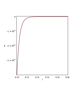
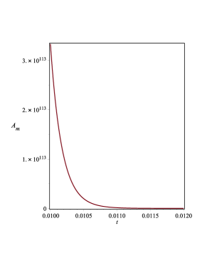
Figure $1(a)$ depicts the variation of pressure versus time for $\lambda=-0.1$, $c_{1}=1.1$, $c_{2}=1$, $\alpha=1$ and $n=0.1$ as a representative case. From the figure we observe that pressure is increasing function of time. It starts from a large negative value and approaches to a small negative value near zero. From the discovery of the accelerated expansion of the universe, it is generally assumed that this cosmic acceleration is due to some kind of energy-matter with negative pressure known as ‘dark energy’.

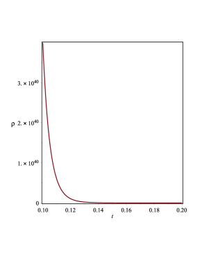
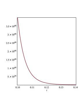
The energy density has been graphed versus time in Fig. $1(b)$. It is evident that the energy density remains always positive and decreasing function of time and it converges to zero as $t\to\infty$ as expected.

The behaviour of the universe in this model will be determined by the cosmological term $\Lambda$, this term has the same effect as a uniform mass density $\rho_{eff}=-\Lambda$ which is constant in time. A positive value of $\Lambda$ corresponds to a negative effective mass density (repulsion). 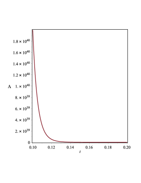Hence, we expect that in the universe with a positive value of $\Lambda$ the expansion will tend to accelerate whereas in the universe with negative value of $\Lambda$ the expansion will slow down, stop and reverse. Figure $1(c)$ is the plot of cosmological term $\Lambda$ versus time. From this figure, we observe that $\Lambda$ is decreasing function of time $t$ and it approaches a small positive value at late time (i.e. at present epoch). Recent cosmological observations [1$-$5, 9, 10] suggest the existence of a positive cosmological constant $\Lambda$ with the magnitude $\Lambda(G\hbar/c^{3})\approx 10^{-123}$. These observations on magnitude and red-shift of type Ia supernova suggest that our universe may be an accelerating one with induced cosmological density through the cosmological $\Lambda$-term. Thus, the nature of $\Lambda$ in our derived models are supported by recent observations. For detailed description via different theoretical models and cosmography tests, one can see the recent review by Bamba et al. [75].

The directional Hubble parameters ($H_{i}$), Hubble parameter ($H$), expansion scalar ($\theta$), spatial volume ($V$), anisotropy parameter ($A_{m}$), shear scalar ($\sigma$) and deceleration parameter ($q$) are, respectively, given by

$$H_{1}=\frac{\alpha}{n}\coth(\alpha t),$$ (63)

$$H_{2}=\frac{\alpha}{n}\coth(\alpha t)+\frac{c_{2}}{\sinh^{\frac{3}{n}}(\alpha t)},$$ (64)

$$H_{3}=\frac{\alpha}{n}\coth(\alpha t)-\frac{c_{2}}{\sinh^{\frac{3}{n}}(\alpha t)},$$ (65)

$$\theta=3H=\frac{3\alpha}{n}\coth(\alpha t),$$ (66)

$$V=ABC=(\sinh(\alpha t))^{\frac{3}{n}},$$ (67)

$$A_{m}=\frac{1}{3}\left(\frac{nc_{2}}{\alpha\coth(\alpha t)\sinh^{\frac{3}{n}}(\alpha t)}\right)^{2}.$$ (68)

$$\sigma^{2}=\left(\frac{c_{2}}{\sinh^{\frac{3}{n}}(\alpha t)}\right)^{2},$$ (69)

$$q=n\left(1-\tanh^{2}(\alpha t)\right)-1.$$ (70)

From the Eq. (70), we observe that $q>0$ for $t<\frac{1}{\alpha}\tanh^{-1}(1-\frac{1}{n})^{\frac{1}{2}}$ and $q<0$ for $t>\frac{1}{\alpha}\tanh^{-1}(1-\frac{1}{n})^{\frac{1}{2}}$. It is also observed that for for $0<n\leq 1$, our model is in accelerating phase but for $n>1$, our model is evolving from decelerating phase to accelerating phase. It follows that in our derived model, one can choose the value of $n$ which gives the physical behavior of DP consistent with the observations. Also, recent observations from SNe Ia, expose that the present universe is accelerating and the value of DP lies to some place in the range $-1\leq q<0$.

For the present Universe ($t_{0}=13.8$ GYr) with $q_{0}=-0.73$ (Cunha [76]), Eq. (70) yields the following relationship between the constants $n$ and $\alpha$:

$$\alpha=\frac{1}{13.8}\tanh^{-1}\left[1-\frac{0.27}{n}\right]^{\frac{1}{2}}.$$ (71)

It is self explanatory from the above relation that for the present Universe, the model is valid only for $n>0.27$. It is observed that for $0<n\leq 1$, our model is in accelerating phase but for $n>1$, our model is evolving from decelerating phase to accelerating phase. It follows that in our derived model, one can choose the value of $n$ which gives the physical behavior of DP consistent with the observations.

From Eqs. (67) and (66), we observe that the spatial volume is zero at $t=0$ and the expansion scalar is infinite, which show that the universe starts evolving with zero volume at $t=0$ which is big bang scenario. From Eqs. (43)$-$(45), we observe that the spatial scale factors are zero at the initial epoch $t=0$ and hence the model has a point type singularity [77]. We observe that proper volume increases exponentially with time. The physical quantities isotopic pressure ($p$), proper energy density ($\rho$), Hubble factor ($H$) and shear scalar ($\sigma$) diverge at $t=0$. As $t\to\infty$, volume becomes infinite where as $p$, $\rho$, $H$, $\theta$ approach to zero. It is important to note here that $\lim_{t\to 0}\left(\frac{\rho}{\theta^{2}}\right)$ spread out to be constant. Therefore, the model of the universe goes up homogeneity and matter is dynamically negligible near the origin. This is in good agreement with the result already given by Collins[78]. Finally, we can say that the model represents a shearing, non-rotating, expanding and accelerating universe, which starts with a big bang singularity and approaches to isotropy at the present epoch.

The dynamics of the mean anisotropic parameter depends on two constant $n$ and $c_{2}$ . From Eq. (68), we observe that at late time when $t\to\infty$, $A_{m}\to 0$. Thus, our model has transition from initial anisotropy to isotropy at present epoch which is in good harmony with current observations. Figure $1(e)$ depicts the variation of anisotropic parameter ($A_{m}$) versus cosmic time $t$. From the figure, we observe that $A_{m}$ decreases with time and tends to zero as $t\to\infty$. Thus, the observed isotropy of the universe can be achieved in our model at present epoch. In the frame of pure $f(R)$ gravity, the pioneer works (Nojiri and Odintsov [79, 80]) present very natural unification of the early-time inflation and late-time acceleration. According to this observation which a is sub-case of current model there is no place for large anisotropy after inflation. But the case in the present model is different. In our derived model $q<0$ for $t>t_{c}$, where the critical time $t_{c}=\frac{1}{\alpha}\tanh^{-1}(1-\frac{1}{n})^{\frac{1}{2}}$. Also we observe that the average scale factor $a(t)\to 0$ as $t\to 0$ and also $a(t)\to\infty$ as $t\to\infty$. This indicates that there exists inflation.

The Ricci scalar for the solution is given by

$$R=-\frac{1}{8n^{2}[\cosh(\alpha t)-1]}\Biggl{[}4\left[c_{2}^{2}(3n+n^{2})+24\alpha^{2}\right]\cosh^{2}(\alpha t)$$

$$+3c_{2}^{2}(n^{2}+9)\cosh^{4}(\alpha t)+2c_{2}^{2}\left(n^{2}+9\right)\cosh^{6}(\alpha t)$$

$$-c_{2}^{2}\left(n^{2}-6n-9\right)\cosh^{8}(\alpha t)+48n^{2}\sinh^{\frac{2n-2}{n}}(\alpha t)-48\alpha^{2}n+4n^{2}c_{2}^{2}\Biggr{]}.$$ (72)

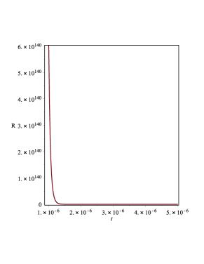
The evolution of Ricci scalar $R$ with cosmic time is shown in Fig. $1(d)$. We observe that the curvature is positive through the whole evolution of the universe and $R\to 0$ as $t\to\infty$ and $R\to\infty$ when $t\to 0$ indicating the initial singularity.

(a) $\rho-p$

(b) $\rho+p$

(c) $\rho+3p$

(d) $v_{s}$

(e) statefinder

Figure 2: The plots of energy conditions, sound speed $\upsilon_{s}$ verses time and also $s$ versus $r$. Here $\lambda=-0.1$, $c_{1}=1.1$, $c_{2}=1$, $\alpha=1$ and $n=0.1$.

5 Physical acceptability of the solutions

For the stability of corresponding solutions, we should check that our model is physically acceptable.
Sound speed:
It is required that the velocity of sound $\upsilon_{s}$ should be less than velocity of light $(c)$. As we are working in the gravitational units with unit speed of light, i.e. the velocity of sound exists within the range $0\leq\upsilon_{s}=\left(\frac{dp}{d\rho}\right)\leq 1$.

We obtain the sound speed as

$$\upsilon_{s}=\frac{dp}{d\rho}=\frac{g(t)}{h(t)},$$ (73)

where

$$g(t)=\lambda\sinh^{\frac{2}{n}}(\alpha t)\Biggl{[}3c_{2}^{2}(n+3)^{2}\cosh^{8}(\alpha t)+24c_{2}^{2}(n+3)\cosh^{6}(\alpha t)$$

$$+9c_{2}^{2}\left(n^{2}+2n+7\right)\cosh^{4}(\alpha t)+6c_{2}^{2}\left(n^{2}+6n+3\right)\cosh^{2}(\alpha t)$$

$$+12nc_{2}^{2}-16n\alpha^{2}\Biggr{]}+16n\sinh^{2}(\alpha t).$$ (74)

and

$$h(t)=\sinh^{\frac{2}{n}}(\alpha t)\Biggl{[}6c_{2}^{2}\lambda(n^{2}+3)\cosh^{2}(\alpha t)+18c_{2}^{2}\lambda\cosh^{2}(\alpha t)$$

$$+9c_{2}^{2}\lambda(n^{2}+9)\cosh^{4}(\alpha t)+(n+3)\cosh^{6}(\alpha t)+3c_{2}^{2}(n+3)^{2}\lambda\cosh^{8}(\alpha t)$$

$$+256\alpha^{2}\pi(n-3)+16\lambda\alpha^{2}(n-6)+512n\pi+80n\lambda\Biggr{]}.$$ (75)

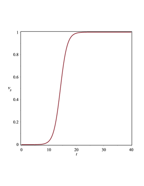
Here we observe that $\upsilon_{s}<1$. Fig. $2(d)$ depicts the plot of sound speed with time. We observe that $\upsilon_{s}<1$ throughout the evolution of the universe.
Energy conditions:
The weak energy conditions (WEC) and dominant energy conditions (DEC) are given by

(i) $\rho\geq 0$,     (ii) $\rho-p\geq 0$     and     (iii) $\rho+p\geq 0$.

The strong energy conditions (SEC) are given by $\rho+3p\geq 0$.

The left hand side of energy conditions have been graphed in Figs. $1(b)~{}\&~{}2(a,b,c)$. From these figures, we observe that

• The WEC and DEC for the derived model are satisfied.

• The SEC is also satisfied.

It has been shown by Wald [81] that under very general conditions all Bianchi cosmologies (except Bianchi IX) with a cosmological constant and an energy momentum tensor satisfying the strong and dominant energy conditions, will unavoidably enter a phase of exponential expansion. With the help of this result Jensen and Stein-Schabes [82] showed that if the number e-folds the Universe expands during its exponential phase is given by N then it will take a time of the order $t\simeq e^{2N}\sqrt{\Lambda}$ for anisotropy to have any effect on the observable universe. One remarkable result is the independence of this result from the type or magnitude of the initial anisotropy.

Statefinder diagnostic:
Sahni et al. [83] have introduced a pair of parameters $\{r,s\}$, called Statefinder parameters. In fact, trajectories in the $\{r,s\}$ plane corresponding to different cosmological models demonstrate qualitatively different behaviour. The statefinder parameters can effectively differentiate between different form of dark energy and provide simple diagnosis regarding whether a particular model fits into the basic observational data. The above statefinder diagnostic pair has the following form:

$$r=1+3\frac{\dot{H}}{H^{2}}+\frac{\ddot{H}}{H^{3}}\;\;\mbox{and}\;\;s=\frac{r-1}{3(q-\frac{1}{2})}\;,$$ (76)

to differentiate among different form of dark energy. Here $H$ is the Hubble parameter and $q$ is the deceleration parameter. The two parameters $\{r,s\}$ are dimensionless and are geometrical since they are derived from the cosmic scale factor $a(t)$ alone, though one can reproduce them in terms of the parameters of dark energy and dark matter. This pair provides information about dark energy in a model$-$independent way, that is, it categorizes dark energy in the context of back-ground geometry only which is not dependent on theory of gravity. Hence, geometrical variables are universal.

For our model, the parameters $\{r,s\}$ can be explicitly written in terms of $t$ as

$$r=\frac{1}{nH^{2}}\left[nH^{2}-3\alpha^{2}csch^{2}(\alpha t)+\alpha^{3}\coth^{2}\{1-2csch^{2}(\alpha t)\}\right],$$ (77)

$$s=\frac{-2}{3nH^{2}(2q-1)}\left[3\alpha^{2}csch^{2}(\alpha t)-\alpha^{3}\coth^{2}\{1+2csch^{2}(\alpha t)\}\right].$$ (78)

So we can get the relation between $r$ and $s$ as

$$s=\frac{1}{3(q-\frac{1}{2})}(r-1).$$ (79)

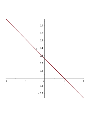
Figure $2(e)$ depicts the variation of $s$ against $r$. From Fig. $2(e)$, we observe that $s$ is negative when $r\geq 1$. The figure shows that the universe starts from an Einstein static era ($r\to\infty,s\to-\infty$) and goes to the $\Lambda$CDM model ($r=1,s=0$).

Therefore, on the basis of above discussions and analysis, our corresponding solutions are physically acceptable.

6 Discussions

Evolution of Bianchi type-$V$ cosmological model is studied in presence of perfect fluid and variable cosmological constant in $f(R,T)$ theory of gravity (Harko et al. [27]). For each choice of the function $f(R,T)$, we get different theoretical models. Three examples have been given in Harko et al. [27] (i) $f(R,T)=R+2f(T)$, (ii) $f(R,T)=f_{1}(R)+f_{2}(T)$ and (iii) $f(R,T)=f_{1}(R)+f_{2}(R)f_{3}(T)$. The cosmological consequences of the case (i) has been discussed before by several authors. In this paper, the gravitational field equation has been established by taking case (ii) into consideration. To find the deterministic solution, we have considered a time dependent deceleration parameter which yields a scale factor as $a(t)=\sinh^{\frac{1}{n}}(\alpha t)$, where $n$ and $\alpha$ are positive constants. For $n>1$, this generates a transition of the universe from the early decelerating phase to the recent accelerating phase.

The current observations of the large-scale cosmic microwave background suggest that our physical universe is expanding isotropic and homogeneous models with a positive cosmological constant. The analysis of CMB fluctuations may confirm this picture. But other analysis reveal some inconsistency. Analysis of WMAP data sets shows that the universe could have a preferred directions (Pullen et al. [84]; Samal et al. [85]; Groeneboom and Eriksen [86]; and Armend$\acute{a}$riz-Pic$\acute{o}$n et al. [87]). The ILC$-$WMAP data maps show seven axes well aligned with one another and the direction Virgo. For this reason Bianchi models are important in the study of anisotropies.

The main features of the models are as follows:

• In summary, we considered the modified gravity which naturally unifies two expansion phases of the universe: inflation at early times and cosmic acceleration at current epoch.

• The models are based on exact solutions of the $f(R,T)$ gravity field equations for the anisotropic Bianchi-V space-time filled with perfect fluid with time dependent $\Lambda$-term.

• The model represents an expanding, shearing, non-rotating and accelerating universe.

• For suitable choice of constants the anisotropic parameter $A_{m}$ tends to zero for sufficiently large time (Fig. $1(e)$). Hence, the present model is isotropic at late time which is consistent to the current observations.

• It has been found that $\Lambda$ is a decreasing function of time and it converges to a small positive value at late time. The nature of decaying vacuum energy density $\Lambda(t)$ in our derived model is supported by recent cosmological observations. These observations on magnitude and red-shift of type Ia supernova suggest that our universe may be an accelerating one with induced cosmological density through the cosmological $\Lambda$-term.

• In literature it is a plebeian practice to consider constant deceleration parameter. Now for a Universe which was decelerated in past and accelerating at present epoch, the DP must show signature flipping as already discussed. Therefore, our consideration of DP to be variable is physically justified. Our derived model is accelerating at present epoch.

• For different choice of $n$, we can generate a class of viable cosmological models of the universe in Bianchi type-V space-time. For example, if we set $n=1$ in Eq. (42), we find $a=\sinh(\alpha t)$ which is used by Pradhan et al. [65] in studying the accelerating dark energy models in Bianchi type-$VI_{0}$ space-time and Pradhan et al. [66] in studying Bianchi type-I cosmological models with time dependent $\Lambda$-term. It is observed that such models are also in good harmony with current observations.

• We observe that our derived solutions are physically acceptable in concordance with the fulfillment of WEC, DEC and SEC. The sound speed $\upsilon_{s}<1$ (see in Fig. $2(d)$). The models in $f(R,T)$ theory of gravity has stability and has initial singularity. Wald [81] pointed out that Bianchi cosmologies (except Bianchi $IX$) with $\Lambda$ and satisfying DEC and SEC will enter in a phase of exponential expansion.

• $\{r,s\}$ diagram (Fig. $2(e)$) shows that the evolution of the universe starts from Einstein static era ($r\to\infty,s\to-\infty$) and approaches to $\Lambda$CDM model ($r=1,s=0$). So, from the Statefinder parameter $\{r,s\}$, the behaviour of different stages of the evolution of the universe have been generated.

Thus, the solutions demonstrated in this paper may be useful for better understanding of the characteristic of Bianchi type-V cosmological models in the evolution of the universe within the framework of $f(R,T)$ gravity theory.

References

- [1] Perlmutter, S., et al. (Supernova Cosmology Project Collaboration): Nature 391, 51 (1998)
- [2] Perlmutter, S., et al. (Supernova Cosmology Project Collaboration): Astrophys. J., 517, 565 (1999)
- [3] Perlmutter, S., et al.: Astrophys. J. 598, 102 (2003)
- [4] Riess, A.G., et al. (Supernova Search Team Collaboration): Astron. J. 116, 1009 (1998)
- [5] Riess, A.G., et al. (Supernova Search Team Collaboration): Astrophys. J., 607, 665 (2004)
- [6] Bennett, C.L., et al.: Astrophys. J. Suppl. 148, 1 (2003)
- [7] Spergel, D.N., et al.: Astrophys. J. Suppl. 148, 175 (2003)
- [8] Tegmark, M., et al.: Astrophys. J. 606 702 (2004)
- [9] Tonry, J.L., et al. (Supernova Search Team Collaboration): Astrophys. J. 594, 1 (2003)
- [10] Clocchiatti, A., et al. (High Z SN Search Collaboration): Astrophys. J. 642, 1 (2006)
- [11] Allen, S.W., et al.: Mon. Not. R. Astron. Soc. 353, 457 (2004)
- [12] Seljak, U., et al.: Phys. Rev. D 71, 103515 (2005)
- [13] Adelman-McCarthy, J.K., et al.: Astrophys. J. Suppl. Ser. 162, 38 (2006)
- [14] Carroll, S.M., Duvvuri, V., Trodden, M., Turner, M.S.: Phys. Rev. D 70, 043528 (2004)
- [15] Capozziello, S., Nojiri, S., Odintsov, S.D., Troisi, A.: Phys. Lett. B 639, 135 (2006)
- [16] Nojiri, S., Odintsov, S.D.: Physical Review D 74, 086005 (2006)
- [17] Hendi, S.H., Momeni, D.: Eur. Phys. J. C 71, 1823 (2011)
- [18] Sharif, M., Arif, S.: Astrophys. Space Sci. 342, 237 (2012)
- [19] Nojiri, S., Odintsov, S.D.: Phys. Lett. B 631, 1 (2005)
- [20] Nojiri, S., Odintsov, S.D.: Phys. Rep. 505, 59 (2011)
- [21] Cognola, G., Gastaldi, M., Zerbini, S.: Int. J. Theor. Phys. 47, 898 (2008)
- [22] Nojiri, S., Odintsov, S.D., Tretyakov, P.V.: Prog. Theor. Phys. Suppl. 172, 81 (2008)
- [23] Garcia, N.M., Lobo, F.S.N., Mimoso, J.P.: arXiv:1012.0953[gr-qc], (2010)
- [24] Bamba, K., Capozziello, S., Nojiri, S., Odintsov, S.D.: Astrophys Space Sci 342, 155 (2012)
- [25] Jamil, M., Momeni, D., Myrzakulov, R.: Eur. Phys. J. C 72, 2137 (2012)
- [26] Jamil, M., Yesmakhanova, K., Momeni, D., Myrzakulov, R.: Cent. Eur. J. Phys. 10(5), 1065 (2012)
- [27] Harko, T., Lobo, F.S.N., Nojiri, S., Odintsov, S.D.: Physical Review D 84, 024020 (2011)
- [28] Chaubey, R., Shukla, A.K.: Astrophys Space Sci 343, 415 (2013)
- [29] Adhav, K.S.: Astrophys. Space Sci 339, 365 (2012)
- [30] Samanta, G.C.: Int. J. Theor. Phys. 52, 2303 (2013)
- [31] Reddy, D.R.K., Santikumar, R., Naidu, R.L.: Astrophys. Space Sci. 342, 249 (2012)
- [32] Reddy, D.R.K., Naidu, R.L., Satyanarayana, B.: Int. J. Theor. Phys. 51, 3222 (2012)
- [33] Reddy, D.R.K., Kumar, R.S., Kumar, T.V.P.: Int. J. Theor. Phys. 52, 239 (2013)
- [34] Hinshaw, G., et al.: Astrophys. J. Suppl. 148, 135 (2003)
- [35] Hinshaw, G., et al.: Astrophys. J. Suppl. 288, 170 (2007)
- [36] Hinshaw, G., et al.: Astrophys. J. Suppl. 180, 225 (2009)
- [37] Jaffe, J., et al.: Astrophys. J. 629, L1 (2005)
- [38] Jaffe, J., et al.: Astrophys. J. 643, 616 (2006)
- [39] Jaffe, J., et al.: Astron. Astrophys. 460, 393 (2006)
- [40] Campanelli, L., Cea, P., Tedesco, L.: Phys. Rev. D 97 131302 (2006)
- [41] Campanelli, L., Cea, P., Tedesco, L.: Phys. Rev. D 76 063007 (2007)
- [42] Hoftuft, J. et al.: Astrophys. J. 699, 985 (2009)
- [43] Guth, A.H.: Phys. Rev. D 23, 347 (1981)
- [44] Sato, K.: Mon. Not. R. Astron. Soc. 195, 467 (1981)
- [45] Albrecht, A., Steinhardt, P.J.: Phys. Rev. Lett. 48, 1220 (1982).
- [46] Linde, A.D.: Phys. Lett. B 108, 389 (1982)
- [47] Linde, A.D.: Phys. Lett. B 129, 177 (1983)
- [48] Linde, A.D.: Phys. Lett. B 259, 38 (1991)
- [49] Linde, A.D.: Phys. Rev. B 49, 748 (1994)
- [50] Barrow, J.D., Turner, M.S.: Nature 292, 35 (1981)
- [51] Steigman, G., Turner, M.S.: Phys. Lett. B 128, 295 (1983)
- [52] Gron, O.: Phys. Rev. D 32, 1598 (1983a)
- [53] Gron, O.: Phys. Rev. D 33, 1204 (1983b)
- [54] Martinez-Gonzalez, E., Jones, B.J.T.: Phys. Lett. B 167, 37 (1983)
- [55] Harko, T., Lobo, F.S.N.: Eur. Phys. J. C 70, 373 (2010)
- [56] Poplawski, N.J.: arXiv:gr-qc/0608031 (2006)
- [57] Samanta, G.C., Dhal, S.N.: Int. J. Theor. Phys. 52, 1334 (2013)
- [58] Shamir, M.F., Jhangeer, A., Bhatti, A.A.: arXiv:1207.0708[gr-qc] (2012)
- [59] Magnano, G.: arXiv:gr-qc/9511027 (1995)
- [60] Poplawski, N.J.: Class. Quantum Grav. 23, 2011 (2006)
- [61] Poplawski, N.J.: Class. Quantum Grav. 23, 4819 (2006)
- [62] Pradhan, A.: Indian J. Phys. DOI: 10.1007/s12648-013-0399-9 (2013). arXiv:1211.1882[physics.gen-ph]
- [63] Pradhan, A., Singh, A.K., Chouhan, D.S.: Palestine J. Math. 3, Issue 1, 130 (3014).
- [64] Chawla, C., Mishra, R.K., Pradhan, A.: Eur. Phys. J. Plus 127, 137 (2012)
- [65] Pradhan, A., Jaiswal, R., Jotania, K., Khare, R.K.: Astrophys. Space Sci. 337, 401 (2012)
- [66] Pradhan, A., Jaiswal, R., Khare, R.K.: Astrophys. Space Sci. 343, 489 (2013)
- [67] Amirhashchi, H., Pradhan, A., Zainuddin, H.: Int. J. Theor. Phys. 50, 3529 (2011)
- [68] Amirhashchi, H., Pradhan, A., Saha, B.: Astrophys. Space Sci. 333, 295 (2011)
- [69] Pradhan, A., Amirhashchi, H.: Astrophys. Space Sci. 332, 441 (2011)
- [70] de Bernardis, P., et al.: Nature 404, 955 (2000)
- [71] Hanany, S. et al.: Astrophys. J. 545, L5 (2000)
- [72] Padmanabhan, T., Roychowdhury, T: Mon. Not. R. Astron. Soc. 344, 823 (2003)
- [73] Amendola, L.: Mon. Not. R. Astron. Soc. 342, 221 (2003).
- [74] Riess, A.G., et al.: Astrophys. J. 560, 49 (2001)
- [75] Bamba, K., Jamil, M., Momeni, D., Myrzakulov, R.: Astrophys. Spacs Sci 344, 259 (2013)
- [76] Cunha, J.V.: Phys. Rev. D 79, 047301 (2009)
- [77] MacCallum, M.A.H.: Commun. Math. Phys. 18, 2116 (1971)
- [78] Collins, C.B.: J. Math. Phys. 18, 2116 (1977)
- [79] Nojiri, S., Odintsov, S.D.: Physical Review D 68, 123512 (2003)
- [80] Nojiri, S., Odintsov, S.D.: Int. J. Geom. Meth. Mod. Phys. 4, 115 (2007)
- [81] Wald, R.M.: Phys. Rev. D 28, 2118 (1983)
- [82] Jensen, L.G., Stein-Schabes, J.A.: FERMI LAB-Pub-86/48-A, March (1986)
- [83] Sahni, V., Saini, T.D., Starobinsky, A.A., Alam, U.: JETP Lett. 77, 201 (2003)
- [84] Pullen, A.R., Kamionkowski, M.: Phys. Rev. D 76, 103529 (2007)
- [85] Samal, P.K., Saha, R., Jain, P., Ralston, J.P.: Mon. Not. R. Astron. Soc. 385, 1718 (2008)
- [86] Groeneboom, N.E., Eriksen, H.K.: Astrophys. J. 690, 1807 (2009)
- [87] Armendriz-Picn, C.: Phys. Rev. Lett. 102, 031301 (2009)