On Periodic Reference Tracking Using Batch-Mode Reinforcement Learning with Application to Gene Regulatory Network Control
Abstract
In this paper, we consider the periodic reference tracking problem in the framework of batch-mode reinforcement learning, which studies methods for solving optimal control problems from the sole knowledge of a set of trajectories. In particular, we extend an existing batch-mode reinforcement learning algorithm, known as Fitted Q Iteration, to the periodic reference tracking problem. The presented periodic reference tracking algorithm explicitly exploits a priori knowledge of the future values of the reference trajectory and its periodicity. We discuss the properties of our approach and illustrate it on the problem of reference tracking for a synthetic biology gene regulatory network known as the generalised repressilator. This system can produce decaying but long-lived oscillations, which makes it an interesting system for the tracking problem. In our companion paper we also take a look at the regulation problem of the toggle switch system, where the main goal is to drive the system’s states to a specific bounded region in the state space.
Index Terms:
batch-mode reinforcement learning; reference tracking; fitted Q iteration; synthetic biology; gene regulatory networks; generalised repressilatorI Introduction
There are many problems in engineering, which require forcing the system to follow a desired periodic reference trajectory (e.g., in repetitive control systems [1]). One approach to solve these problems is to define first a distance between the state of the system and the desired reference point at time . Then explicitly seek for a control policy that minimises this distance for all subject to problem specific constraints. In the case of systems in the Euclidean state-space, for example, the Euclidean distance can be used.
In this paper, we are interested in solving reference tracking problems of discrete-time systems using an optimal control approach. In our setting, the dynamics of the system is only known in the form of one-step system transitions. A one-step system transition is a triplet , where denotes a successor state of the system in state subjected to input . Inference of near-optimal policies from one-step system transitions is the central question of batch-mode reinforcement learning [2, 3]. Note that reinforcement learning [4] focuses on a more general problem of policy inference from interactions with the system. Usually, in batch-mode reinforcement learning, very few assumptions are made on the structure of the control problem. This gives batch-mode reinforcement learning algorithms a high degree of flexibility in comparison with other control methods. Batch-mode reinforcement learning has had numerous applications in many disciplines such as engineering [5], HIV treatment design [6], and medicine [7]. In this paper, one batch-mode reinforcement learning algorithm is considered, namely the Fitted Iteration algorithm [8]. This algorithm focuses on the computation of a so called function, which is used to compute a near-optimal control policy. The algorithm computes the function using an iterative procedure based on the Bellman equation, a regression method and the collected samples of system trajectory.
The focus of this paper is an extension of the Fitted Iteration to the reference tracking problem. In our extension, we explicitly take into account the future reference trajectory values and the period . Moreover, regression is separated into independent regression problems, which can save computational effort. The algorithm is implemented in Python using open-source packages and libraries [9], [10], [11], [12].
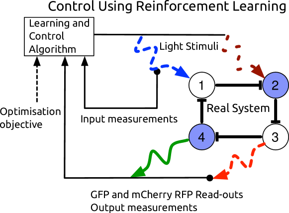
To illustrate our reference tracking method, we consider its application to a synthetic biology gene regulatory network known as the generalised repressilator. The repressilator is a ring of three mutually repressing genes pioneered in [13], and theoretically generalised to rings consisting of more than three genes in [14]. Repression is an interaction between two genes, such that the protein product of the repressing gene prevents protein expression of the repressed gene. Or simply put, where one gene can turn off the other. A generalised repressilator with a sufficiently large, even number of genes (such as the four-gene ring in Figure 1) can exhibit decaying but very long-lived oscillations [15]. The objective of this paper is to force one or several protein concentrations to follow a priori defined reference trajectories, namely: sinusoids and ramps. A deeper background on synthetic biology and its control applications is provided in our companion paper [16].
The paper is organised as follows. Section II covers batch-mode reinforcement learning. In Section III, an extension of the Fitted Iteration to the reference tracking problem is presented. In Section IV our illustrative application, reference tracking for the generalised repressilator system, is given. Finally, Section V concludes the paper.
II Fitted Iteration
II-A Problem Formulation
Consider a deterministic discrete-time dynamical system
| (1) |
where the bold values stand for vectors with elements , is the state of the system at time , and is a control input, which at each time belongs to a compact set . Consider also, associated with this dynamical system, an optimal control problem, which is defined in terms of the minimisation of an infinite sum of discounted costs :
where is a mapping from the state-space onto , which is called the feedback control policy, and is a positive constant smaller than one, which is called the discount factor. For the purpose of this paper, it is assumed that is a given function. The goal is to compute the optimal policy based only on one-step transitions of the system (1). One-step system transitions are given as a set , where denotes a successor state of the system in state subjected to input (if the function is known then is simply equal to ).
II-B Algorithm
The central object in Fitted Iteration is the function, which is defined as follows:
The main idea of the approach is to exploit the celebrated Bellman equation
| (2) |
which provides a convenient expression for the computation of the optimal feedback control policy:
| (3) |
The Bellman equation can be theoretically solved using an iterative procedure
where and is the unique solution to (2) due to the fact that is a contraction mapping (cf. [3]). However in the continuous state-space case, this iterative procedure is hard to solve, especially when only the one-step system transitions in are given. The Fitted Q iteration algorithm computes, from the sole knowledge of a sequence of functions , , that approximates the sequence , , . Let and for every in compute:
| (4) |
This expression gives only for , in , while the entire function is estimated using a regression algorithm (e.g., EXTRA Trees [17]). Now the iterative procedure is derived by generalising (4) as follows:
| (5) |
where at each step is estimated using a regression algorithm. If the iteration procedure stops at the iteration number , an approximate policy can be computed as follows:
| (6) |
Inputs: Set of one-step system transitions , cost , stopping criterion
Outputs: Policy
A simple stopping criterion can be, for example, an a priori fixed maximum number of iterations . The value is chosen such that is sufficiently small and, hence, the values are not modified significantly for larger than . Other, more advanced, stopping criteria are described in [8]. The resulting iterative method is outlined in Algorithm 1. A major property of the fitted iteration algorithm is convergence. This is understood as convergence of to a fixed state-action value function given a fixed set as grows to infinity. It was shown in [8], that under certain conditions Algorithm 1 converges and it is possible to estimate in advance the distance between and the iterate .
III Periodic Reference Tracking Using the Fitted Iteration Algorithm
III-A Problem Formulation
Consider, a system:
| (7) | ||||
where the function is unknown. The function , however, is a known periodic function of period , and the variable takes only a finite number of values . Hence, is equal to for all smaller than , and is equal to . The reference tracking problem is defined as follows:
| (8) | ||||
| subject to | ||||
where is a given instantaneous cost function, is a function defining the distance between the current state and reference , and is a feedback control policy. In order to track the reference , reducing the value of the cost must reduce the distance . The instantaneous cost can optionally depend on the control signal and the states in order to provide additional constraints in the state-space and/or control action space. As for the Fitted Iteration, the control policy is inferred based solely on the trajectories given in the form of one-step system transitions , where denotes a successor state of the system in state subjected to input .
III-B Algorithm
The variable can be seen as an additional state in the extended state-space . Based on this extended state-space we can derive the Bellman equation for the tracking problem and the following iterative procedure for the computation of the function:
| (9) |
where is equal to . It can be shown that this iterative procedure has a unique solution based on a similar contraction mapping argument as in the previous section. Hence the optimal policy in the extended state-space is computed as:
The input set to the algorithm normally consists of the one-step system transitions . However, since our state-space has been extended to include , should now include as well. Since the time evolution of is known a priori we can simply modify the set as follows , where and . This will effectively copy times the training set . Now given this modification, we can proceed to the computational procedure. As before is equal to and the next iterates can be obtained according to:
| (10) |
According to the Fitted Q Iteration framework, every function must be estimated by a regression algorithm, which uses the input set and the corresponding values of the approximated function . This input set can grow significantly, if the period of the reference trajectory is large, which can render a regression algorithm computationally intractable. For example, with only a thousand one-step system transitions and period equal to , the total number of samples is equal to . Therefore, it is proposed to break up the regression of into independent regression problems, one for every function . This can be done, because the evolution of the variable is known in advance and takes a finite number of values. To make these ideas more transparent, (10) is rewritten using a different notation as follows:
| (11) |
where stands for the function . For every value , the regression algorithm will approximate the function by using the input set and the corresponding values . Thus the initial regression problem is indeed separated into independent problems.
Our approach can be also seen as a modification of the function approximator. The first layer of our approximator is a deterministic branching according to the values . After that a regression algorithm is performed to approximate the functions as prescribed. Finally, if the iterative procedure has stopped at iteration , a near-optimal policy can be computed as follows:
| (12) |
Inputs: Sets of one-step system transitions , function and reference values , cost , stopping criterion
Outputs: Policy
Our approach is outlined in Algorithm 2. Periodicity is a crucial assumption, since the period of the reference trajectory corresponds to the number of different functions built in this algorithm. Convergence of Algorithm 2 can be established using the following lemma.
Lemma 1
To prove this lemma, we have to make sure that the approximator of the functions will not break the convergence proof in [8]. Only one modification in this approximator is made, which is the deterministic branching in its first layer according to . It can be shown that this modification does not violate the convergence arguments in [8].
III-C Other Applications of the Algorithm
The presented algorithm addresses the problem of optimal control of the system (7), where a part of the dynamics is known and a part of the dynamics is to be learned. In our setting, the known dynamics describe a reference trajectory, which takes only a finite number of values. However, there are other problems for which Algorithm 2 can be useful. Consider the system, where describes the system dynamics and is known:
| (13) | ||||
The function could be a model of an actuator or some dynamics of the system, e.g., a time-delay in the control signal. In the latter case, the function delays the application of the control action by a number of time samples. If takes a finite number of values, then the problem can be solved using Algorithm 2 without major modifications.
Another application is a system with dynamics and a given feedforward compensator , which helps to counteract the measured disturbance :
| (14) | ||||
IV Tracking of Periodic Trajectories by the Generalized Repressilator
IV-A System Description
As an illustrative application of our method we consider the problem of periodic reference tracking for a six gene generalised repressilator system. There are two major species associated with every gene (the mRNA and protein concentrations), which results in a twelve state system. Throughout the section we adopt the following notation: denotes the protein concentration produced by the translation of mRNA of gene . By definition of the generalised repressilator, the transcription of mRNA is repressed by the previous gene expression product in the network. With a slight abuse of notation, we assume that is equal to in order to model the cyclic structure of the generalised repressilator. The dynamics of the generalised repressilator system can be described by the following set of deterministic equations:
| (15) | ||||
where is an integer from one to six, and is equal to one, if is equal to , and equal to zero otherwise. We consider a control scheme similar to the one used for the toggle switch regulation problem (see our companion paper [16]), where the light control signals induce the expression of genes through the activation of their photo-sensitive promoters. The control signal only acts on the mRNA dynamics of gene , whereas the control signal only acts on the mRNA dynamics of gene . The influence of the light signals on the rate of mRNA production of genes and is denoted by and , respectively. To simplify the system dynamics and as it is usually done for the repressilator model [13], we consider the corresponding parameters of the mRNA and protein dynamics for different genes to be equal. Hence, the trajectories will be very similar between the different genes. For the purpose of this paper, we chose:
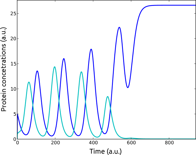
As shown in [15], this system exhibits a long-lived oscillatory behaviour around an unstable limit cycle as depicted in Figure 2. The “natural” period of these slowly decaying oscillations is around arbitrary time units.
IV-B Algorithm Parameters and Implementation
The instantaneous cost function is defined differently based on the considered example. In the first case, the objective is for the concentration of protein to track an a priori specified reference trajectory. In the other cases, the objective is for the concentrations of two proteins and to track their respective reference trajectories. When tracking of two protein concentrations needs to be ensured, the cost function will depend on these two protein concentrations and and on the corresponding references and . Note that here and in the sequel stands for the -th element of the vector . When tracking needs to be ensured for only one protein concentration (i.e., ), the cost function will only depend on and the scalar reference . In both cases, the cost depends on the control signals in order to penalise the use of light stimuli and thus minimise the metabolic burden caused by heterologous gene expression. The cost is defined using a distance between the observed state and the reference trajectories :
where will be equal to one or zero depending on how many reference trajectories we want to track simultaneously.
The discount factor is equal to , the choice of which is guided by considerations similar to the ones in [8]. The stopping criterion is simply a bound on the number of iterations, which for the purpose of this paper is . The set of system transitions is generated according to the following procedure. system trajectories starting in a random initial state are generated. The control actions applied to generate the trajectories are random as well. Every trajectory has at most samples. These state transitions are then gathered in the set . At every step every function is approximated using the regression algorithm EXTremly RAndomized Trees (EXTRA Trees), which was shown to be an effective regression algorithm for the fitted iteration framework [17]. The parameters for the algorithm are set to the default values from [8].
IV-C Results
IV-C1 One sinusoidal reference trajectory, different periods
In this example, we are going to force the concentration of the protein to track a sinusoid with different periods. The parameter is set to zero and the sinusoid is chosen to resemble the natural oscillations in terms of amplitude and mean value:
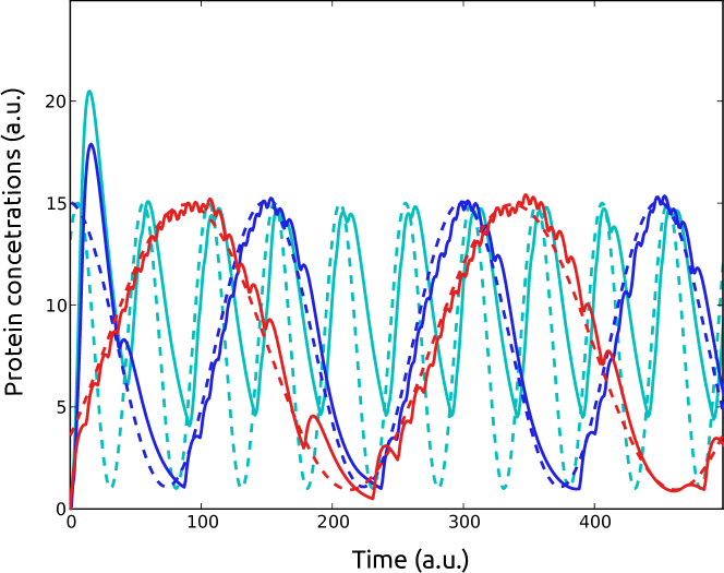
We are testing the algorithm for the following periods , , . We can increase the concentration of the protein directly trough application of the control signal . We can also decrease the concentration of the protein through increasing the concentration of the protein , which acts as a repressor for gene . The results of several experiments are depicted in Figure 3. The natural oscillations have a period of approximately arbitrary time units, therefore the blue dashed curve is easiest to follow. Using repression by gene , the algorithm manages to find a schedule of light pulses that allows to track the dotted red curve, even though the period is much larger than . However, due to the inherent dynamics of the system, the algorithm cannot bring down the concentration of protein fast enough to properly track the cyan curve. The repression by gene is not strong enough in this case to allow accurate tracking. It is important to remark that tracking of the trajectory by protein results in damping of the oscillations in the other proteins and mRNA dynamics.
IV-C2 Two sinusoidal reference trajectories
For this experiment we chose two sinusoids (i.e., is equal to one), where the second sinusoid lags behind the first one:
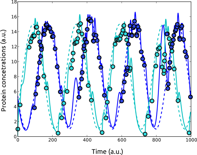
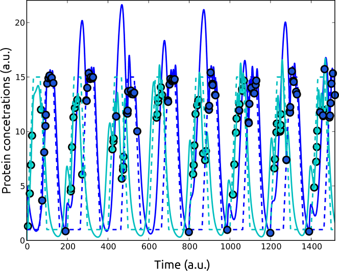
Genes, their protein products and the corresponding reference trajectories are colour coded in this example: the blue colour corresponds to protein and the cyan colour corresponds to protein . The “blue” gene represses the “cyan” one, hence an increase in the “blue” protein concentration can be used to decrease the concentration of the “cyan” protein. However, the concentration of the “blue” protein cannot be decreased directly. The sinusoids are chosen with approximate knowledge of the natural oscillation dynamics: in terms of amplitude and mean value of oscillations. Their period is chosen equal to time samples. As depicted in Figure 4, the algorithm can force the concentration of the first two proteins to follow both sinusoids. Moreover, numerous experiments were conducted starting from different initial conditions, which yielded similar tracking results after the initial transient period had elapsed. It is worth noting the interesting behaviour exhibited by the “blue” protein concentration: At some point the protein concentration starts growing without any light stimulation. This can be explained by the repressilator oscillatory dynamics, where the protein’s concentration can grow periodically. Moreover, since the “blue” protein concentration cannot be decreased directly it can grow significantly as can be observed during the time range between and time units. It also means that controlling this system with a larger period will be harder due to this fast growth of the “blue” protein concentration induced by the dynamics of the system.
IV-C3 Two ramp reference trajectories
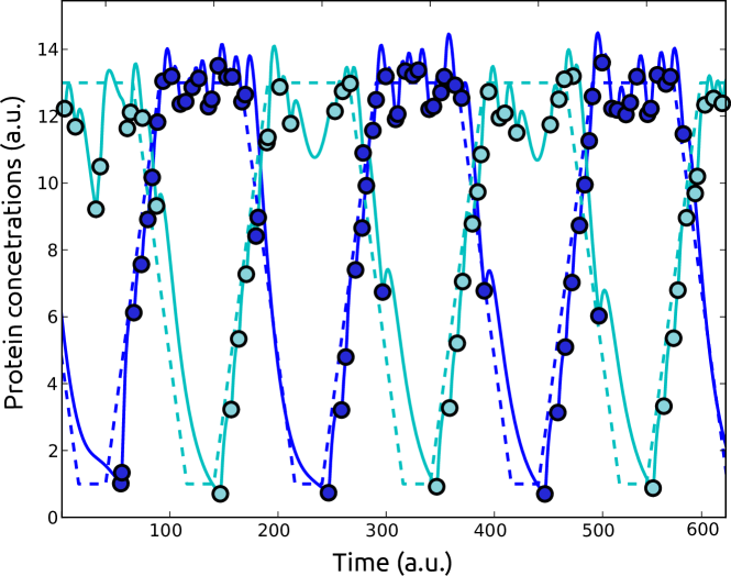
The two ramp tracking setting is very similar to the two sinusoids tracking setting. However, in the situation depicted in upper panel of Figure 5 unsuccessful simultaneous tracking of two ramps is occurring. The reasons for such a behaviour are the same as above. The difference is that they are more pronounced in this case due to large time intervals during which a low reference value needs to be followed by one of the proteins. Note that the first ramp is followed almost perfectly by both protein concentrations. However, after a long time interval of low reference value, the concentration of the “blue” protein starts to grow due the inherent dynamics of the system. With a modified ramp such behaviour disappears as depicted in the lower panel of Figure 5. Even though tracking is not perfect, the algorithm manages to find an approximate solution to the optimal control problem, which is quite remarkable given the very limited amount of information provided by the input-output data in such setting.
V Discussion and Conclusion
In this paper, we have presented a periodic reference tracking reinforcement learning algorithm. The algorithm is based on the established fitted Q iteration framework, and inherits its properties. The proposed algorithm makes full use of the fact that the reference trajectory is known in advance, which results in better sample efficiency in comparison with other approaches proposed in the literature.
The algorithm is illustrated on the problem of tracking a periodic trajectory for the generalised repressilator system. This system has received considerable attention from the synthetic and systems biology community due to its ability to produce long-lived oscillatory behaviours. The algorithm was able to find near optimal solutions to the periodic tracking reference problem, even when the period of the reference trajectory was smaller than the natural period of oscillation of the system.
References
- [1] Shinji Hara, Yutaka Yamamoto, Tohru Omata, and Michio Nakano. Repetitive control system: a new type servo system for periodic exogenous signals. Automatic Control, IEEE Tran on, 33(7):659–668, 1988.
- [2] R. Fonteneau, S.A. Murphy, L. Wehenkel, and D. Ernst. Batch mode reinforcement learning based on the synthesis of artificial trajectories. Annals of Operations Research, pages 1–34, 2012.
- [3] L. Buşoniu, R. Babuška, B. De Schutter, and D. Ernst. Reinforcement Learning and Dynamic Programming Using Function Approximators. CRC Pr I Llc, 2010.
- [4] R.S. Sutton and A.G. Barto. Reinforcement Learning, an Introduction. MIT Press, 1998.
- [5] Martin Riedmiller. Neural fitted q iteration–first experiences with a data efficient neural reinforcement learning method. Machine Learning: ECML 2005, pages 317–328, 2005.
- [6] G.-B. Stan, F. Belmudes, R. Fonteneau, F. Zeggwagh, M.-A. Lefebvre, C. Michelet, and D. Ernst. Modelling the influence of activation-induced apoptosis of CD4+ and CD8+ T-cells on the immune system response of a HIV-infected patient. IET Systems Biology, 2(2):94–102, 2008.
- [7] Susan A Murphy. Optimal dynamic treatment regimes. Journal of the Royal Statistical Society: Series B (Statistical Methodology), 65(2):331–355, 2003.
- [8] D. Ernst, P. Geurts, and L. Wehenkel. Tree-based batch mode reinforcement learning. Journal of Machine Learning Research, 6:503–556, April 2005.
- [9] Fabian Pedregosa, Gaël Varoquaux, Alexandre Gramfort, Vincent Michel, Bertrand Thirion, Olivier Grisel, Mathieu Blondel, Peter Prettenhofer, Ron Weiss, Vincent Dubourg, et al. Scikit-learn: Machine learning in python. The Journal of Machine Learning Research, 12:2825–2830, 2011.
- [10] Joblib: running python function as pipeline jobs. http://packages.python.org/joblib.
- [11] J. D. Hunter. Matplotlib: A 2d graphics environment. Computing In Science & Engineering, 9(3):90–95, 2007.
- [12] Eric Jones, Travis Oliphant, Pearu Peterson, et al. SciPy: Open source scientific tools for Python. 2001–, http://www.scipy.org/.
- [13] M.B. Elowitz and S. Leibler. A synthetic oscillatory network of transcriptional regulators. Nature, 403(6767):335–338, 2000.
- [14] H. Smith. Oscillations and multiple steady states in a cyclic gene model with repression. J Math Biol, 25(15):169–190, Jul 1987.
- [15] Natalja Strelkowa and Mauricio Barahona. Switchable genetic oscillator operating in quasi-stable mode. J R Soc Interface, 7(48):1071–1082, 2010.
- [16] A. Sootla, N. Strelkowa, D. Ernst, M. Barahona, and G.B. Stan. Toggling the genetic switch using reinforcement learning. In submission to the 52nd Conf. on Decision and Control, Dec. 2013, http://www3.imperial.ac.uk/people/a.sootla/publications.
- [17] Pierre Geurts, Damien Ernst, and Louis Wehenkel. Extremely randomized trees. Machine Learning, 63(1):3–42, 2006.