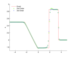
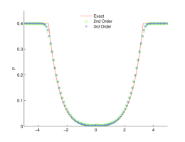
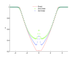
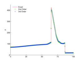
The generalized Riemann problems for hyperbolic balance laws: A unified formulation towards high order111Jianzhen Qian is supported by Postdoctoral Science Foundation of China No. 2012M510366; Jiequan Li is supported by NSFC with Nos. 91130021 and 11031001; Shuanghu Wang is supported by NSFC with No. 91130021.

Jianzhen Qian qianjzmath@gmail.com Jiequan Li jiequan@bnu.edu.cn Shuanghu Wang wang_shuanghu@iapcm.ac.cn Institute of Applied Physics and Computational Mathematics, Beijing 100088, China School of Mathematical Science, Beijing Normal University, Beijing, 100875, P. R. China Key Laboratory of Computational Physics, Institute of Applied Physics and Computational Mathematics, Beijing 100088, China
Abstract

The Generalized Riemann Problems (GRP) for nonlinear hyperbolic systems of balance laws in one space dimension are now well-known and can be formulated as follows: Given initial-data which are smooth on two sides of a discontinuity, determine the time evolution of the solution near the discontinuity. In particular, the GRP of (k+1)𝑘1(k+1)th order high-resolution is based on an analytical evaluation of the time derivative up to k𝑘kth order, which turns out to be dependent only on the spatial derivatives up to k𝑘kth order. While the classical Riemann problem serves as a primary “building block” in the construction of many numerical schemes (most notably the Godunov scheme), the analytic study of GRP will lead to an array of “GRP schemes”, which extend the Godunov scheme. Currently there are extensive studies on the second-order GRP scheme, which proves to be robust and is capable of resolving complex multidimensional fluid dynamic problems [M. Ben-Artzi and J. Falcovitz, “Generalized Riemann Problems in Computational Fluid Dynamics”, Cambridge University Press, 2003]. More general formulation of the second-order GRP solver can be found in [Numer. Math. (2007) 106:369-425], but still confined with a class of “weakly coupled systems”. In this paper, we provide a unified approach for solving the GRP in the general context of hyperbolic balance laws, without weakly coupled constraint, towards high order accuracy. The derivation of the second-order GRP solver is more concise compared to those in previous works and the third-order GRP (or quadratic GRP) is resolved for the first time. The latter is shown to be necessary through numerical experiments with strong discontinuities. Our method relies heavily on the new treatment of the rarefaction wave. Indeed, as a main technical step, the “propagation of singularities” argument for the rarefaction fan, is simplified by deriving the L(Q)-equations, an ODE system for the “evolution” of the “characteristic derivatives” in x𝑥x-t𝑡t space for generalized Riemann invariants, with aid of the generalized characteristic coordinates. The case of a sonic point is incorporated into a general treatment. The accuracy of the derived GRP solvers are justified and numerical examples are presented for the performance of the resulting scheme.

keywords:
Generalized Riemann problem , Hyperbolic balance laws , GRP solver , Riemann invariants

1 Introduction

In this paper we consider the generalized Riemann problem (GRP) for hyperbolic balance laws

Ut+F(U)x=H(x,U),𝑈𝑡𝐹𝑈𝑥𝐻𝑥𝑈\frac{\partial U}{\partial t}+\frac{\partial F(U)}{\partial x}=H(x,U), (1.1)

where U=(u1,,um)𝑈subscript𝑢1subscript𝑢𝑚U=(u_{1},\cdots,u_{m}) is the unknown variable with F=(f1,,fm)𝐹subscript𝑓1subscript𝑓𝑚F=(f_{1},\cdots,f_{m}) being the flux functions, and H(x,U)𝐻𝑥𝑈H(x,U) is a source term resulting from geometrical or physical effects, x𝑥x is the spatial variable and t𝑡t is the time variable. In this study, we will concentrate on the numerical aspect of (1.1), rather than important theoretical issues such as well-posedness and solution structures.

In the development of numerical techniques approximating solutions of (1.1), the finite volume scheme plays absolutely indispensable role, wherein one of most crucial ingredients is the construction of numerical fluxes and it boils down to the resolution of associated (generalized) Riemann problems at each computational cell interface. Specifically, we denote by Ij=[xj1/2,xj+1/2]subscript𝐼𝑗subscript𝑥𝑗12subscript𝑥𝑗12I_{j}=[x_{j-1/2},x_{j+1/2}], Δx=xj+1/2xj1/2Δ𝑥subscript𝑥𝑗12subscript𝑥𝑗12\Delta x=x_{j+1/2}-x_{j-1/2}, the computational cell numbered j𝑗j, and by {tn}n=0superscriptsubscriptsubscript𝑡𝑛𝑛0\{t_{n}\}_{n=0}^{\infty} the sequence of discretized time levels, Δt=tn+1tnΔ𝑡subscript𝑡𝑛1subscript𝑡𝑛\Delta t=t_{n+1}-t_{n}. The finite volume scheme is then constructed by integrating the governing equations (1.1) both in space and time over the control volume Ij×[tn+1,tn]subscript𝐼𝑗subscript𝑡𝑛1subscript𝑡𝑛I_{j}\times[t_{n+1},t_{n}], yielding

Ujn+1=UjnΔtΔx(Fj+1/2nFj1/2n)+ΔtHjn,superscriptsubscript𝑈𝑗𝑛1superscriptsubscript𝑈𝑗𝑛Δ𝑡Δ𝑥superscriptsubscript𝐹𝑗12𝑛superscriptsubscript𝐹𝑗12𝑛Δ𝑡superscriptsubscript𝐻𝑗𝑛U_{j}^{n+1}=U_{j}^{n}-\frac{\Delta t}{\Delta x}\big{(}F_{j+1/2}^{n}-F_{j-1/2}^{n}\big{)}+\Delta tH_{j}^{n}, (1.2)

where

Ujn=1Δxxj1/2xj+1/2U(x,tn)dxsuperscriptsubscript𝑈𝑗𝑛1Δ𝑥superscriptsubscriptsubscript𝑥𝑗12subscript𝑥𝑗12𝑈𝑥subscript𝑡𝑛differential-d𝑥U_{j}^{n}=\frac{1}{\Delta x}\int_{x_{j-1/2}}^{x_{j+1/2}}U(x,t_{n})\,\mathrm{d}x (1.3)

is the average of U(x,tn)𝑈𝑥superscript𝑡𝑛U(x,t^{n}) over the cell Ijsubscript𝐼𝑗I_{j}. The remaining terms in (1.2), Fj+1/2nsuperscriptsubscript𝐹𝑗12𝑛F_{j+1/2}^{n} and Hjnsuperscriptsubscript𝐻𝑗𝑛H_{j}^{n} , are the temporal average of F(U(x,t))𝐹𝑈𝑥𝑡F(U(x,t)) along the interface x=xj+1/2𝑥subscript𝑥𝑗12x=x_{j+1/2} and the space-time integral average of the source H(x,U)𝐻𝑥𝑈H(x,U), i.e.,

Fj+1/2n=1Δttntn+1F(U(xj+11,t))dt,superscriptsubscript𝐹𝑗12𝑛1Δ𝑡superscriptsubscriptsubscript𝑡𝑛subscript𝑡𝑛1𝐹𝑈subscript𝑥𝑗11𝑡differential-d𝑡\displaystyle F_{j+1/2}^{n}=\frac{1}{\Delta t}\int_{t_{n}}^{t_{n+1}}F(U(x_{j+\frac{1}{1}},t))\,\mathrm{d}t, (1.4)
Hjn=1ΔtΔxtntn+1xj1/2xj+1/2H(x,U)dxdt.superscriptsubscript𝐻𝑗𝑛1Δ𝑡Δ𝑥superscriptsubscriptsubscript𝑡𝑛subscript𝑡𝑛1superscriptsubscriptsubscript𝑥𝑗12subscript𝑥𝑗12𝐻𝑥𝑈differential-d𝑥differential-d𝑡\displaystyle H_{j}^{n}=\frac{1}{\Delta t\Delta x}\int_{t_{n}}^{t_{n+1}}\int_{x_{j-1/2}}^{x_{j+1/2}}H(x,U)\,\mathrm{d}x\,\mathrm{d}t. (1.5)

A numerical scheme is obtained if one can supply suitable approximation for Fj+1/2nsuperscriptsubscript𝐹𝑗12𝑛F_{j+1/2}^{n} and Hjnsuperscriptsubscript𝐻𝑗𝑛H_{j}^{n} with given data U(x,tn)𝑈𝑥subscript𝑡𝑛U(x,t_{n}) at t=tn𝑡subscript𝑡𝑛t=t_{n}. Formally, for the Godunov-type schemes, this usually consists the following three procedures.

  1. A

    Data reconstruction: Based on the cell average values Ujnsuperscriptsubscript𝑈𝑗𝑛U_{j}^{n}, reconstruct the initial data U(x,tn)𝑈𝑥subscript𝑡𝑛U(x,t_{n}) as piece-wise smooth distribution, being constant or polynomial in each cell Ijsubscript𝐼𝑗I_{j}.

  2. B

    Solution evolution: Solve the (generalized) Riemann problem at each cell interface x=xj+1/2𝑥subscript𝑥𝑗12x=x_{j+1/2} to evolve the solution.

  3. C

    Numerical approximation: Take the numerical integration in (1.4) and (1.5) to get Fj+1/2nsuperscriptsubscript𝐹𝑗12𝑛F_{j+1/2}^{n} and Sjnsuperscriptsubscript𝑆𝑗𝑛S_{j}^{n} under suitable CFL condition.

[Uncaptioned image]

For the notable Godunov scheme [10] and higher order schemes using Riemann solvers such as MUSCL [24, 25] and TVD [11] schemes, the classical Riemann problem is solved in each cell interface to evolve the solution from tnsuperscript𝑡𝑛t^{n} to tn+1superscript𝑡𝑛1t^{n+1}. The corresponding initial data are taken as interface limit values of U(tn,x)𝑈subscript𝑡𝑛𝑥U(t_{n},x) in the neighboring cells. As an extension, the GRP scheme assumes the piecewise smooth initial data and evolves solutions by analytically solving the generalized Riemann problem at each cell interface with at least second order accuracy. Currently, the second-order GRP scheme has already been exploited and put into use for several compressible fluid models [1, 2, 3, 4, 5, 6, 16, 27, 28]. Let us now outline a standard process for its implementation. Assume the data at time t=tn𝑡superscript𝑡𝑛t=t^{n} is piece-wise linear with slope σjnsuperscriptsubscript𝜎𝑗𝑛\sigma_{j}^{n}, i.e. on Ijsubscript𝐼𝑗I_{j} we have

U(x,tn)=Ujn+σjn(xxj),x(xj1/2,xj+1/2).formulae-sequence𝑈𝑥superscript𝑡𝑛superscriptsubscript𝑈𝑗𝑛superscriptsubscript𝜎𝑗𝑛𝑥subscript𝑥𝑗𝑥subscript𝑥𝑗12subscript𝑥𝑗12U(x,t^{n})=U_{j}^{n}+\sigma_{j}^{n}(x-x_{j}),\quad x\in(x_{j-1/2},x_{j+1/2}). (1.6)

Then the Godnuov-type scheme of second order takes the form

Ujn+1=UjnΔtΔx(Fj+1/2n+1/2Fj1/2n+1/2)+Δt2(Hj+1/2n+1/2+Hj1/2n+1/2),superscriptsubscript𝑈𝑗𝑛1superscriptsubscript𝑈𝑗𝑛Δ𝑡Δ𝑥superscriptsubscript𝐹𝑗12𝑛12superscriptsubscript𝐹𝑗12𝑛12Δ𝑡2superscriptsubscript𝐻𝑗12𝑛12superscriptsubscript𝐻𝑗12𝑛12U_{j}^{n+1}=U_{j}^{n}-\frac{\Delta t}{\Delta x}\big{(}F_{j+1/2}^{n+1/2}-F_{j-1/2}^{n+1/2}\big{)}+\frac{\Delta t}{2}\big{(}H_{j+1/2}^{n+1/2}+H_{j-1/2}^{n+1/2}\big{)}, (1.7)

where the following notations are used

Fj+1/2n+1/2=F(Uj+1/2n+1/2),Hj+1/2n+1/2=H(xj+1/2,Uj+1/2n+1/2),formulae-sequencesuperscriptsubscript𝐹𝑗12𝑛12𝐹superscriptsubscript𝑈𝑗12𝑛12superscriptsubscript𝐻𝑗12𝑛12𝐻subscript𝑥𝑗12superscriptsubscript𝑈𝑗12𝑛12F_{j+1/2}^{n+{1/2}}=F\big{(}U_{j+1/2}^{n+1/2}\big{)},\quad H_{j+1/2}^{n+1/2}=H\big{(}x_{j+1/2},U_{j+1/2}^{n+1/2}\big{)}, (1.8)

and Uj+1/2n+1/2superscriptsubscript𝑈𝑗12𝑛12U_{j+1/2}^{n+1/2} is the mid-point value or the average of U(xj+1/2,t)𝑈subscript𝑥𝑗12𝑡U(x_{j+1/2},t) over time interval [tn,tn+1]subscript𝑡𝑛subscript𝑡𝑛1[t_{n},t_{n+1}]. For simplicity, the source term is currently discretized with an interface method, which is the trapezoidal rule in space and the mid-point rule in time [4, 13] in order to keep second order accuracy. The central issue is how to obtain the mid-point value Uj+1/2n+1/2superscriptsubscript𝑈𝑗12𝑛12U_{j+1/2}^{n+1/2}, which is formally approximated by the Taylor expansion (ignoring the higher order terms)

Uj+1/2n+1/2Uj+1/2n+Δt2(Ut)j+1/2n,superscriptsubscript𝑈𝑗12𝑛12superscriptsubscript𝑈𝑗12𝑛Δ𝑡2superscriptsubscript𝑈𝑡𝑗12𝑛U_{j+1/2}^{n+{1/2}}\cong U_{j+1/2}^{n}+\frac{\Delta t}{2}\left(\frac{\partial U}{\partial t}\right)_{j+1/2}^{n}, (1.9)

where

Uj+1/2n=limttn+0U(xj+1/2,t),(Ut)j+1/2n=limttn+0Ut(xj+1/2,t).formulae-sequencesuperscriptsubscript𝑈𝑗12𝑛subscript𝑡subscript𝑡𝑛0𝑈subscript𝑥𝑗12𝑡superscriptsubscript𝑈𝑡𝑗12𝑛subscript𝑡subscript𝑡𝑛0𝑈𝑡subscript𝑥𝑗12𝑡U_{j+1/2}^{n}=\lim_{t\rightarrow t_{n}+0}U(x_{j+1/2},t),\quad\left(\frac{\partial U}{\partial t}\right)_{j+1/2}^{n}=\lim_{t\rightarrow t_{n}+0}\frac{\partial U}{\partial t}(x_{j+1/2},t). (1.10)

The value Uj+1/2nsuperscriptsubscript𝑈𝑗12𝑛U_{j+1/2}^{n} is obtained by solving the associated Riemann problem for the homogeneous hyperbolic conservation laws as used in the (first order) Godunov scheme [10]. The main ingredient lies upon the calculation of the instantaneous time derivative (Ut)j+1/2nsuperscriptsubscript𝑈𝑡𝑗12𝑛(\frac{\partial U}{\partial t})_{j+1/2}^{n}. Even in the Godunov scheme, the time derivative (Ut)j+1/2nsuperscriptsubscript𝑈𝑡𝑗12𝑛(\frac{\partial U}{\partial t})_{j+1/2}^{n} should be properly treated once the source term is present, which makes the solution evolve non-uniformly.

For the solution U𝑈U being smooth near the grid point (xj+1/2,tn)subscript𝑥𝑗12subscript𝑡𝑛(x_{j+1/2},t_{n}), it follows directly from (1.1) that

(Ut)j+1/2n=FU(Uj+1/2n)(Ux)j+1/2n+H(xj+1/2,Uj+1/2n).superscriptsubscript𝑈𝑡𝑗12𝑛𝐹𝑈superscriptsubscript𝑈𝑗12𝑛superscriptsubscript𝑈𝑥𝑗12𝑛𝐻subscript𝑥𝑗12superscriptsubscript𝑈𝑗12𝑛\left(\frac{\partial U}{\partial t}\right)_{j+1/2}^{n}=-\frac{\partial F}{\partial U}\left(U_{j+1/2}^{n}\right)\left(\frac{\partial U}{\partial x}\right)_{j+1/2}^{n}+H\big{(}x_{j+1/2},U_{j+1/2}^{n}\big{)}. (1.11)

However, for the generalized Riemann problem including singularity at grid point (xj+1/2,tn)subscript𝑥𝑗12subscript𝑡𝑛(x_{j+1/2},t_{n}), (1.11) is no longer valid, even for scalar cases, because there exists nonlinear waves (rarefaction waves or discontinuities) issuing from the singularity point (xj+1/2,tn)subscript𝑥𝑗12subscript𝑡𝑛(x_{j+1/2},t_{n}). Indeed, thinking of the initial data (1.6) with non-zero slopes as a perturbation of piecewise constant Riemann initial data and the source term S(x,U)𝑆𝑥𝑈S(x,U) as a perturbation of the homogenous system of equations, the GRP solution is a perturbation of that of the associated Riemann problem at least in the neighborhood of the singularity point. It turns out that the GRP solution consists of, for a short time following the “disintegration” of initial discontinuity, the curvilinear rarefaction wave and the discontinuities (contact discontinuity or shock wave) with time varying speed [4, Chap. 5].

The solution U𝑈U together with its derivatives may undergo a jump discontinuity across each wave. Hence, in order to solve the generalized Riemann problem, it requires one to explore the mode of the discontinuity for the derivatives coming along with each wave, which is in fact described by a set of linear algebraic equations. This bears an analogy to the resolution of classical Riemann problem, which involves exploring the relation, usually described by a one parameter curve, between the two states of U𝑈U connected by each wave. Indeed, the treatment for capturing the discontinuities of the derivatives across each type of waves can be sketched out as follows.

  1. A

    Since the generalized Riemann invariants are transported in the transversal direction of the rarefaction fan, it is natural to use them for studying the variation of the derivatives across the rarefaction wave. Actually, the directional (emanating characteristic direction) derivatives of the generalized Riemann invariants are determined by their values on either side of the wave.

  2. B

    The generalized Riemann invariants, which remain continuous across corresponding contact discontinuities, are differentiated in the direction of the discontinuity (characteristic).

  3. C

    For the shock wave, the identities implied by the Rankine-Hugoniot conditions are differentiated along the shock trajectories.

As indicated in the previous works, the most technical step lies on the treatment for rarefaction fan, which relies on the analysis in term of “characteristic coordinates”.

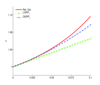
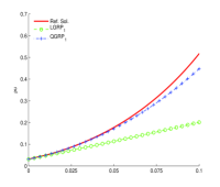
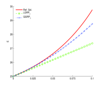
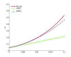
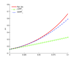
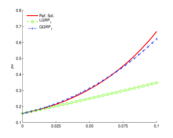
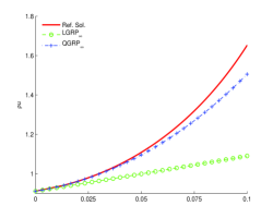
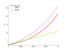
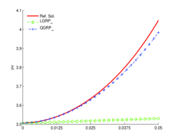
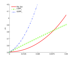
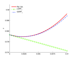
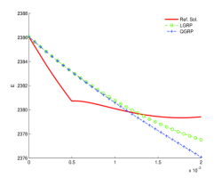
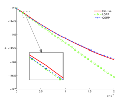
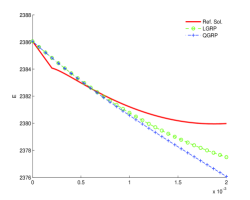
The methodology for resolving the generalized Riemann problem is originated in [1, 2, 3], wherein the original GRP is designed for the compressible fluid flows with two related Lagrangian and Eulerian versions. See also the recent textbook [4] for detailed discussions. The Eulerian version is always derived by using the Lagrangian case. The transformation is quite delicate, particularly for sonic cases, because it becomes singular at sonic points. The direct Eulerian version, more flexible for applications, is developed recently in the context of shallow water equations [16], planar compressible fluid and the compressible fluid flows [5, 6]. The approach for solving GRP therein, being ready to handle any strict hyperbolic system endowed with a coordinate system of Riemann invariants (in particular, the two equations system), is extended to handle more general weakly coupled systems (in the sense of [6, Def. 21]) having only a “partial set” of Riemann invariants. The common point of the above systems is that the generalized Riemann invariants (GRI) are coupled in a manner that enables a “diagonalized” treatment. Although many physical systems, including the compressible fluids flow system, belong to such a class of systems, the existing methods for deriving a second-order GRP solver are rather complicated, which prevents it from practical use in many ways. For example, the treatment of rarefaction relies heavily on the explicit formulation of the Asymptotic Characteristic Coordinate (ACC), which depends on the EOS (equation of state) of the fluid in turn and is sometimes hard to derive. Besides the ACC is not easy to be written out explicitly for higher order GRP solvers that are particularly useful in capturing the propagation of entropy wave [20] (see also Fig. 8.4). Other closely related efforts can be found in [7, 14] using the approach of asymptotic analysis for the resolution of generalized Riemann problems, and in [12, 23, 8] (and the references therein) for approximate Godunov-type high order solvers. The solvers in [23, 8] corresponds to the acoustic case and they fails for resolving strong discontinuities, even with very high order accuracy (this point is confirmed through a numerical experiment Fig. 7.4). Hence it is absolutely necessary to develop the high order (at least third order) GRP scheme by resolving nonlinear wave patterns each computational grid point analytically, in addition to provide an acoustic approximation as the jump there is weak.

Therefore we present a unified approach in this paper, still direct Eulerian, to resolve the GRP for general systems of hyperbolic balance laws (1.1). The weakly coupled constraint is not required here. The solver for second-order GRP (linear GRP) as well as third-order (quadratic GRP) are derived. This paper provides a simplified treatment for the main step, resolution of the rarefaction fan. Indeed, it is carried out by first deriving the system of transport equations for the generalized Riemann invariants and then deriving the “evolution” equations, labeled as the L(Q)-equations, for their characteristic derivatives in x𝑥x-t𝑡t space with aid of the generalized characteristic coordinate (GCC). This is based on the following observations. These characteristic derivatives, and hence the resulting “evolution” equations for them, are independent of the choice of the auxiliary GCC. Thus the explicit expression of the GCC is not required. More importantly, only in the emanating characteristic direction do the derivatives of the GRI (the solution U𝑈U) of any order exist and remain continuous across rarefaction fans. No additional assumption is required for the regularity of the solution U𝑈U. Indeed, the above observations are the reasons why we can derive the third-order (or higher order) GRP solver without many difficulties. By referring to Section 4 for the resolution of the contact discontinuity and the shock wave, the spatial derivatives of the solution, from which the instantaneous time derivatives follow, are obtained by solving a simple system of linear equations in the intermediate regions of the waves. The case of sonic point is handled by supplementing an additional freedom using the differential relation of U𝑈U along the emanating characteristic direction. A special case frequently occur during the numerical application of the GRP scheme is the acoustic case: the initial values of U𝑈U are continuous at the singularity point. This case is comparatively easy to handle and requires less computation cost.

Although this paper focus on exploring solvers for the second-order linear GRP and the third-order quadratic GRP, higher order GRP solvers can be derived with the same methodology and a multidimensional extension can be pursued in a forthcoming work [17]. The resulting GRP solvers consist of two steps: (i) the classical Riemann solver; (ii) calculation of instantaneous time derivatives of U𝑈U. As indicated by the solvers, Step (ii) can be straightforward once the full Riemann solution is obtained. Besides, in both steps, only the limiting values of U𝑈U and its spatial derivatives at two side of the singularity are used, and the resulting linear (resp. quadratic) GRP solver leads to second (resp. third) order accuracy in time approximation to U𝑈U regardless its initial distribution.

This paper is arranged as follows. In Section 2, a basic setup for the system and the GRP are presented. The resolution of rarefaction wave and discontinuity waves, including the contact discontinuity and shock wave, are detailed in Sections 3 and 4, respectively. We conclude the resolution of GRP in Section 5 and the acoustic approximation in Section 6. As an application example, in Section 7, we derive the GRP solvers for compressible variable duct flow system and show the solvers’ accuracy by several tests. Finally, in Section 8, the GRP solvers are used to construct one-step high order numerical scheme and a few 1-D numerical test cases are presented.

2 Basic setup for the system and the GRP

As a basic setup, we assume (1.1) is hyperbolic in the sense that the Jacobian A(U)=F(U)U𝐴𝑈𝐹𝑈𝑈A(U)=\frac{\partial F(U)}{\partial U} of F(U)𝐹𝑈F(U) has m𝑚m eigenvalues

λ1λ2λm.subscript𝜆1subscript𝜆2subscript𝜆𝑚\lambda_{1}\leq\lambda_{2}\leq\cdots\leq\lambda_{m}. (2.1)

The set of left (right) eigenvectors Lksubscript𝐿𝑘L_{k} (Rksubscript𝑅𝑘R_{k}) (associated with λksubscript𝜆𝑘\lambda_{k}, k=1,,m𝑘1𝑚k=1,\cdots,m) are linearly independent. The k𝑘kth characteristic field λksubscript𝜆𝑘\lambda_{k} can be either genuinely nonlinear in the sense of UλkRk0subscript𝑈subscript𝜆𝑘subscript𝑅𝑘0\nabla_{U}\lambda_{k}\cdot R_{k}\neq 0, or linearly degenerate UλkRk=0subscript𝑈subscript𝜆𝑘subscript𝑅𝑘0\nabla_{U}\lambda_{k}\cdot R_{k}=0.

Now let us state the generalized Riemann problem. It is defined as the initial-value problem for system (1.1), subject to the initial data

U(x,0)={P+(x)ifx<0,P(x)ifx>0,𝑈𝑥0casessubscript𝑃𝑥if𝑥0subscript𝑃𝑥if𝑥0U(x,0)=\left\{\begin{array}[]{ll}P_{+}(x)&\text{if}\ x<0,\\ P_{-}(x)&\text{if}\ x>0,\end{array}\right. (2.2)

where P±(x)subscript𝑃plus-or-minus𝑥P_{\pm}(x) are vectors, whose components are the smooth functions. As illustrated in Section 1, the initial structure of the solution is determined by the associated Riemann problem:

{UAt+F(UA)x=0,UA(x,0)=U±,±x>0,casessuperscript𝑈𝐴𝑡𝐹superscript𝑈𝐴𝑥0formulae-sequencesuperscript𝑈𝐴𝑥0subscript𝑈plus-or-minusplus-or-minus𝑥0\left\{\begin{array}[]{l}\frac{\partial U^{A}}{\partial t}+\frac{\partial F(U^{A})}{\partial x}=0,\\[5.69054pt] U^{A}(x,0)=U_{\pm},\quad\pm x>0,\end{array}\right. (2.3)

where U±subscript𝑈plus-or-minusU_{\pm} are the limiting values of P±(x)subscript𝑃plus-or-minus𝑥P_{\pm}(x) at x=0𝑥0x=0, i.e. U±=P±(0±)subscript𝑈plus-or-minussubscript𝑃plus-or-minussuperscript0plus-or-minusU_{\pm}=P_{\pm}(0^{\pm}). We call the solution of (2.3) the associated Riemann solution of (1.1) and (2.2).

Assumption 2.1

The Riemann problem (2.3) is uniquely solvable, and the solution to (2.3) consists of m𝑚m waves Γ1,Γ2,,ΓmsubscriptΓ1subscriptΓ2subscriptΓ𝑚\Gamma_{1},\Gamma_{2},\cdots,\Gamma_{m}. The wave ΓksubscriptΓ𝑘\Gamma_{k}(1km1𝑘𝑚1\leq k\leq m) is an admissible shock, a contact discontinuity, or a rarefaction wave associated with the k𝑘kth characteristic field λksubscript𝜆𝑘\lambda_{k}.

Note that the above assumption does not mean we are confined with strict hyperbolic systems that endowed with distinct eigenvalues.

Denote by RA(x/t,U,U+)superscript𝑅𝐴𝑥𝑡subscript𝑈subscript𝑈R^{A}(x/t,U_{-},U_{+}) the Riemann solution of (2.3). Then we have the following proposition.

Proposition 2.1

Let U(x,t)𝑈𝑥𝑡U(x,t) be the solution to the generalized Riemann problem (1.1) and (2.2). Then for every fixed direction θ=x/t𝜃𝑥𝑡\theta=x/t,

limt0U(θt,t)=RA(θ,U,U+).subscript𝑡0𝑈𝜃𝑡𝑡superscript𝑅𝐴𝜃subscript𝑈subscript𝑈\lim_{t\rightarrow 0}U(\theta t,t)=R^{A}(\theta,U_{-},U_{+}). (2.4)

This implies that the wave configuration for the generalized Riemann problem(1.1) and (2.2) is the same as that for the associated Riemann problem (2.3) around the singularity (x,t)=(0,0+)𝑥𝑡0superscript0(x,t)=(0,0^{+}).

Proposition 2.1 is illustrated schematically in Fig.2.1. The solution of (2.3) is self-similar, and hence the waves are centered. Correspondingly, the waves for (1.1) are curved (See [4] for more detailed descriptions).

Refer to caption
Refer to caption
Figure 2.1: Wave configurations: (a) Wave patterns for the GRP with initial data U(0,x)=P(x)𝑈0𝑥subscript𝑃𝑥U(0,x)=P_{-}(x) for x<0𝑥0x<0 and U(0,x)=P+(x)𝑈0𝑥subscript𝑃𝑥U(0,x)=P_{+}(x) for x>0𝑥0x>0, U±=P±(0±)subscript𝑈plus-or-minussubscript𝑃plus-or-minussuperscript0plus-or-minusU_{\pm}=P_{\pm}(0^{\pm}). (b) Wave patterns for the associated Riemann problem.

We emphasize that the solution U𝑈U is smooth in the intermediate regions of these waves and along each emanating characteristic curve in the rarefaction fan (up to the singularity (0,0+)0superscript0(0,0^{+})). To approximate U𝑈U along t𝑡t-axis with k𝑘kth order accuracy, we can use the Taylor expansion

U(x=0,t)=U(0,0+)+=1k1!Ut(0,0+)(tk)+𝒪(tk+1).𝑈𝑥0𝑡𝑈0superscript0superscriptsubscript1𝑘1superscript𝑈superscript𝑡0superscript0superscript𝑡𝑘𝒪superscript𝑡𝑘1U(x=0,t)=U(0,0^{+})+\sum_{\ell=1}^{k}\frac{1}{\ell!}\frac{\partial^{\ell}U}{\partial t^{\ell}}(0,0^{+})(t^{k})+\mathcal{O}(t^{k+1}). (2.5)

A solver of the GRP is actually that of evaluating the instantaneous time derivatives

Ut(0,0+)=limt0Ut(0,t),t>0.formulae-sequencesuperscript𝑈superscript𝑡0superscript0subscript𝑡0superscript𝑈superscript𝑡0𝑡𝑡0\frac{\partial^{\ell}U}{\partial t^{\ell}}(0,0^{+})=\lim_{t\rightarrow 0}\frac{\partial^{\ell}U}{\partial t^{\ell}}(0,t),\quad t>0. (2.6)

For convenience, we label the problem of evaluating (2.6) with =11\ell=1 (resp. =1,212\ell=1,2) as the linear GRP (resp. quadratic GRP), or LGRP (reps. QGRP) for short. As mentioned in the introduction, this paper concentrates on QGRP.

3 Resolution of curved rarefaction waves

As pointed out earlier, the main feature of the GRP is the resolution of rarefaction waves and the main ingredients are the Riemann invariants and characteristic coordinates. Let us consider to first derive the set of transport equations for the (generalized) Riemann invariants in a general setting. For this purpose, we rewrite (1.1) as a nonconservative form

Ut+A(U)Ux=H(x,U),𝑈𝑡𝐴𝑈𝑈𝑥𝐻𝑥𝑈\frac{\partial U}{\partial t}+A(U)\frac{\partial U}{\partial x}=H(x,U), (3.1)

by recalling A(U)=F(U)/U𝐴𝑈𝐹𝑈𝑈A(U)=\partial F(U)/\partial U. Multiplying (3.1) by L=(L1,,Lm)𝐿subscript𝐿1subscript𝐿𝑚L=(L_{1},\cdots,L_{m}) from the left, it follows that

LUt+ΛLUx=LH(x,U),𝐿𝑈𝑡Λ𝐿𝑈𝑥𝐿𝐻𝑥𝑈L\frac{\partial U}{\partial t}+\Lambda L\frac{\partial U}{\partial x}=LH(x,U), (3.2)

where Λ=diag(λ1,,λm)Λdiagsubscript𝜆1subscript𝜆𝑚\Lambda=\textrm{diag}(\lambda_{1},\cdots,\lambda_{m}). If there exists a set of variables w=(w1,,wm)wsubscript𝑤1subscript𝑤𝑚\textbf{{w}}=(w_{1},\cdots,w_{m}) satisfying wkULkconditionalsubscript𝑤𝑘𝑈subscript𝐿𝑘\frac{\partial w_{k}}{\partial U}\parallel L_{k} (k=1,,m𝑘1𝑚k=1,\cdots,m), then (3.2) is equivalent to

wt+Λwx=LH(x,U).w𝑡Λw𝑥𝐿𝐻𝑥𝑈\frac{\partial\textbf{{w}}}{\partial t}+\Lambda\frac{\partial\textbf{{w}}}{\partial x}=LH(x,U). (3.3)

Indeed, w is a complete set of Riemann invariants. Unfortunately, most of the systems (1.1) with m>2𝑚2m>2, including the full system of compressible Euler equations, do not admit such a set of Riemann invariants. We thus turn to exploring the generalized Riemann invariants (GRI).

3.1 The generalized Riemann invariants (GRI)

Let w=(w1,,wm1)wsubscript𝑤1subscript𝑤𝑚1\textbf{{w}}=(w_{1},\cdots,w_{m-1}) be the generalized Riemann invariants of the k𝑘kth characteristic field. By recalling the definition of GRI [22], we have

UwRk=0,=1,,m1.formulae-sequencesubscript𝑈subscript𝑤subscript𝑅𝑘01𝑚1\nabla_{U}w_{\ell}\cdot R_{k}=0,\quad\ell=1,\cdots,m-1.

Hence, there exists an invertible (m1)×(m1)𝑚1𝑚1(m-1)\times(m-1) matrix K𝐾K, such that

KUw=(L1,,Lk1,Lk+1,,Lm)T=:L(k).K\nabla_{U}\textbf{{w}}=(L_{1},\cdots,L_{k-1},L_{k+1},\cdots,L_{m})^{T}=:L^{(k)}. (3.4)

Multiply (3.1) by KUw𝐾subscript𝑈wK\nabla_{U}\textbf{{w}} from the left yields the following proposition.

Proposition 3.1

Let w=(w1,,wm1)wsubscript𝑤1subscript𝑤𝑚1\textbf{{w}}=(w_{1},\cdots,w_{m-1}) be the GRI of the k𝑘kth characteristic field. Then in any smooth region of U𝑈U there holds

wt+B(k)(U)wx=L(k)H(x,U),w𝑡superscript𝐵𝑘𝑈w𝑥superscript𝐿𝑘𝐻𝑥𝑈\frac{\partial\textbf{{w}}}{\partial t}+B^{(k)}(U)\frac{\partial\textbf{{w}}}{\partial x}=L^{(k)}H(x,U), (3.5)

where

B(k)(U)=K1Λ(k)K,Λ(k)=diag(λ1,,λk1,λk+1,,λm)T,formulae-sequencesuperscript𝐵𝑘𝑈superscript𝐾1superscriptΛ𝑘𝐾superscriptΛ𝑘diagsuperscriptsubscript𝜆1subscript𝜆𝑘1subscript𝜆𝑘1subscript𝜆𝑚𝑇B^{(k)}(U)=K^{-1}\Lambda^{(k)}K,\quad\Lambda^{(k)}=\textrm{diag}(\lambda_{1},\cdots,\lambda_{k-1},\lambda_{k+1},\cdots,\lambda_{m})^{T}, (3.6)

and K𝐾K is determined by (3.4).

Roughly speaking, Proposition 3.1 implies that the generalized Riemann invariants of the k𝑘kth characteristic field are transported along the direction different from λksubscript𝜆𝑘\lambda_{k}. The following useful corollary is straightforward from Proposition 3.1 for the resolution of rarefaction wave. See Remark 3.1 (ii) below.

Corollary 3.1

Let ΓksubscriptΓ𝑘\Gamma_{k} be a characteristic curve associated with λksubscript𝜆𝑘\lambda_{k}. If U𝑈U is continuous and piecewise smooth with ΓksubscriptΓ𝑘\Gamma_{k} being a weak discontinuity curve, then w/tw𝑡{\partial\textbf{{w}}}/{\partial t} and w/xw𝑥{\partial\textbf{{w}}}/{\partial x} in Proposition 3.1 remain continuous across ΓksubscriptΓ𝑘\Gamma_{k}.

3.2 Generalized characteristic coordinates (GCC)

As mentioned in the introduction, the characteristic coordinates, defined as the integral curves of the characteristic equations, play an important role in the resolution of rarefaction waves. In the region of a rarefaction fan, they work similarly to the usual polar coordinates to single out singularities.

Assume that ΓksubscriptΓ𝑘\Gamma_{k} is a rarefaction wave associated with λksubscript𝜆𝑘\lambda_{k} and denote by UL(x,t)subscript𝑈𝐿𝑥𝑡U_{L}(x,t) (resp. UR(x,t)subscript𝑈𝑅𝑥𝑡U_{R}(x,t)) the state U𝑈U on its left (resp. right) side. See Fig. 3.1. To simplify notations, we write λ𝜆\lambda and B𝐵B below for λksubscript𝜆𝑘\lambda_{k} and B(k)superscript𝐵𝑘B^{(k)} in Proposition 3.1, respectively, for a fixed k𝑘k.

Let Csuperscript𝐶C^{-}: β(x,t)=β𝛽𝑥𝑡𝛽\beta(x,t)=\beta and C+superscript𝐶C^{+}: α(x,t)=α𝛼𝑥𝑡𝛼\alpha(x,t)=\alpha, β[βL,βR]𝛽subscript𝛽𝐿subscript𝛽𝑅\beta\in[\beta_{L},\beta_{R}], α<0𝛼0-\infty\leq\alpha<0 be the integral curves of the following equations, respectively,

dxdt=λ,dxdt=μ.formulae-sequenced𝑥d𝑡𝜆d𝑥d𝑡𝜇\frac{\mathrm{d}x}{\mathrm{d}t}=\lambda,\quad\frac{\mathrm{d}x}{\mathrm{d}t}=\mu. (3.7)

Here, different from the previous works [1, 2, 3, 4, 5, 6], μ𝜇\mu in (3.7) is not required to be an eigenvalue of A(U)𝐴𝑈A(U). In fact, it can be the slope of any family of transversal curves different from λ𝜆\lambda. For example, μ=tx𝜇𝑡𝑥\mu=-\frac{t}{x}. The GCC used here is a relaxed version of the afore-mentioned ACC. Moreover, β𝛽\beta and α𝛼\alpha are denoted as follows: β𝛽\beta is the initial value of the slope λ𝜆\lambda at the singularity (x,t)=(0,0)𝑥𝑡00(x,t)=(0,0) and α𝛼\alpha for the transversal characteristic curves is the x𝑥x-coordinates of the intersection point with the leading β𝛽\beta-curve: β=βL𝛽subscript𝛽𝐿\beta=\beta_{L}.

Refer to caption
Figure 3.1: Generalized characteristic coordinates in a rarefaction fan ΓksubscriptΓ𝑘\Gamma_{k}.

The coordinates (x,t)𝑥𝑡(x,t) in the “triangle” sector of the centered rarefaction wave shown in Fig. 3.1 can be expressed in terms of α𝛼\alpha and β𝛽\beta,

x=x(α,β),t=t(α,β),formulae-sequence𝑥𝑥𝛼𝛽𝑡𝑡𝛼𝛽x=x(\alpha,\beta),\quad t=t(\alpha,\beta), (3.8)

which satisfy

xα=λtα,xβ=μtβ.formulae-sequence𝑥𝛼𝜆𝑡𝛼𝑥𝛽𝜇𝑡𝛽\frac{\partial x}{\partial\alpha}=\lambda\frac{\partial t}{\partial\alpha},\quad\frac{\partial x}{\partial\beta}=\mu\frac{\partial t}{\partial\beta}. (3.9)

Denote

Dλ=t+λx,Dμ=t+μx.formulae-sequencesubscript𝐷𝜆𝑡𝜆𝑥subscript𝐷𝜇𝑡𝜇𝑥D_{\lambda}=\frac{\partial}{\partial t}+\lambda\frac{\partial}{\partial x},\quad D_{\mu}=\frac{\partial}{\partial t}+\mu\frac{\partial}{\partial x}. (3.10)

Then we have

α=tαDλ,β=tβDμ.formulae-sequence𝛼𝑡𝛼subscript𝐷𝜆𝛽𝑡𝛽subscript𝐷𝜇\frac{\partial}{\partial\alpha}=\frac{\partial t}{\partial\alpha}D_{\lambda},\quad\frac{\partial}{\partial\beta}=\frac{\partial t}{\partial\beta}D_{\mu}. (3.11)

In particular, as α=0𝛼0\alpha=0, we have

λβ(0,β)=1,tβ(0,β)=0,βLββR.formulae-sequence𝜆𝛽0𝛽1formulae-sequence𝑡𝛽0𝛽0subscript𝛽𝐿𝛽subscript𝛽𝑅\frac{\partial\lambda}{\partial\beta}(0,\beta)=1,\quad\frac{\partial t}{\partial\beta}(0,\beta)=0,\quad\beta_{L}\leq\beta\leq\beta_{R}. (3.12)

Here we remind that, as a basic assumption in Section 2, the solution U𝑈U is smooth along each characteristic curve C:β=β¯:superscript𝐶𝛽¯𝛽C^{-}:\beta=\bar{\beta} inside a rarefaction fan up to the singularity and DλUsubscriptsuperscript𝐷𝜆𝑈D^{\ell}_{\lambda}U, for any 11\ell\geq 1, takes finite value at α=0𝛼0\alpha=0.

It follows, by differentiating the first equation in (3.9) with respect to β𝛽\beta, the second with respect to α𝛼\alpha and then subtracting, that the function t=t(α,β)𝑡𝑡𝛼𝛽t=t(\alpha,\beta) satisfies

(μλ)2tαβ=λβtαμαtβ.𝜇𝜆superscript2𝑡𝛼𝛽𝜆𝛽𝑡𝛼𝜇𝛼𝑡𝛽\displaystyle(\mu-\lambda)\frac{\partial^{2}t}{\partial\alpha\partial\beta}=\frac{\partial\lambda}{\partial\beta}\frac{\partial t}{\partial\alpha}-\frac{\partial\mu}{\partial\alpha}\frac{\partial t}{\partial\beta}. (3.13)

Setting α=0𝛼0\alpha=0 and using (3.12), one obtains

β[tα(0,β)]=1μλtα(0,β).𝛽delimited-[]𝑡𝛼0𝛽1𝜇𝜆𝑡𝛼0𝛽\displaystyle\frac{\partial}{\partial\beta}\left[\frac{\partial t}{\partial\alpha}(0,\beta)\right]=\frac{1}{\mu-\lambda}\frac{\partial t}{\partial\alpha}(0,\beta). (3.14)

We continue to make differentiation of (3.13) with respect to α𝛼\alpha to obtain

(μλ)3tα2β=𝜇𝜆superscript3𝑡superscript𝛼2𝛽absent\displaystyle(\mu-\lambda)\frac{\partial^{3}t}{\partial\alpha^{2}\partial\beta}= α(μλ)2tαβ+2λαβtα+λβ2tα2𝛼𝜇𝜆superscript2𝑡𝛼𝛽superscript2𝜆𝛼𝛽𝑡𝛼𝜆𝛽superscript2𝑡superscript𝛼2\displaystyle-\frac{\partial}{\partial\alpha}(\mu-\lambda)\frac{\partial^{2}t}{\partial\alpha\partial\beta}+\frac{\partial^{2}\lambda}{\partial\alpha\partial\beta}\frac{\partial t}{\partial\alpha}+\frac{\partial\lambda}{\partial\beta}\frac{\partial^{2}t}{\partial\alpha^{2}}
2μα2tβμα2tαβ.superscript2𝜇superscript𝛼2𝑡𝛽𝜇𝛼superscript2𝑡𝛼𝛽\displaystyle\hskip 42.67912pt-\frac{\partial^{2}\mu}{\partial\alpha^{2}}\frac{\partial t}{\partial\beta}-\frac{\partial\mu}{\partial\alpha}\frac{\partial^{2}t}{\partial\alpha\partial\beta}. (3.15)

Recalling (3.12) and (3.14) as well as noticing

2αβλ=β(tαDλλ)=2tαβDλλ+tαβ(Dλλ),superscript2𝛼𝛽𝜆𝛽𝑡𝛼subscript𝐷𝜆𝜆superscript2𝑡𝛼𝛽subscript𝐷𝜆𝜆𝑡𝛼𝛽subscript𝐷𝜆𝜆\displaystyle\frac{\partial^{2}}{\partial\alpha\partial\beta}\lambda=\frac{\partial}{\partial\beta}\left(\frac{\partial t}{\partial\alpha}D_{\lambda}\lambda\right)=\frac{\partial^{2}t}{\partial\alpha\partial\beta}D_{\lambda}\lambda+\frac{\partial t}{\partial\alpha}\frac{\partial}{\partial\beta}\left(D_{\lambda}\lambda\right),

we take α=0𝛼0\alpha=0 to obtain

β[2tα2(0,β)]=𝛽delimited-[]superscript2𝑡superscript𝛼20𝛽absent\displaystyle\frac{\partial}{\partial\beta}\left[\frac{\partial^{2}t}{\partial\alpha^{2}}(0,\beta)\right]= 1μλ2tα2(0,β)+2Dλμλ(tα)2(0,β)1𝜇𝜆superscript2𝑡superscript𝛼20𝛽2subscript𝐷𝜆𝜇𝜆superscript𝑡𝛼20𝛽\displaystyle\frac{1}{\mu-\lambda}\frac{\partial^{2}t}{\partial\alpha^{2}}(0,\beta)+\frac{2D_{\lambda}}{\mu-\lambda}\left(\frac{\partial t}{\partial\alpha}\right)^{2}(0,\beta)
+1μλβ(Dλλ)(tα)2(0,β).1𝜇𝜆𝛽subscript𝐷𝜆𝜆superscript𝑡𝛼20𝛽\displaystyle+\frac{1}{\mu-\lambda}\frac{\partial}{\partial\beta}\left(D_{\lambda}\lambda\right)\left(\frac{\partial t}{\partial\alpha}\right)^{2}(0,\beta). (3.16)

The equations (3.14) and (3.2), for t/α(0,β)𝑡𝛼0𝛽{\partial t}/{\partial\alpha}(0,\beta) and 2t/α2(0,β)superscript2𝑡superscript𝛼20𝛽{\partial^{2}t}/{\partial\alpha^{2}}(0,\beta) repectively, are crucial for deriving the L(Q)𝐿𝑄L(Q)-equations in next subsection.

3.3 The L(Q)𝐿𝑄L(Q)-equations

In this subsection, we shall derive the linear differential ordinary equations for Dλw(0,β)subscript𝐷𝜆w0𝛽D_{\lambda}\textbf{{w}}(0,\beta) and Dλ2w(0,β)superscriptsubscript𝐷𝜆2w0𝛽D_{\lambda}^{2}\textbf{{w}}(0,\beta) with respect to β𝛽\beta, namely, the L𝐿L-equations and Q𝑄Q-equations, respectively, of the GRI. Precisely, we have the following proposition.

Proposition 3.2 (L(Q)𝐿𝑄L(Q)-equations)

The w in Proposition 3.1 satisfies the L𝐿L-equations:

β[Dλw(0,β)]=(λIB)1(DλwL(k)H),𝛽delimited-[]subscript𝐷𝜆w0𝛽superscript𝜆𝐼𝐵1subscript𝐷𝜆wsuperscript𝐿𝑘𝐻\frac{\partial}{\partial\beta}\big{[}D_{\lambda}\textbf{{w}}(0,\beta)\big{]}=(\lambda I-B)^{-1}\big{(}D_{\lambda}\textbf{{w}}-L^{(k)}H\big{)}, (3.17)

and the Q𝑄Q-equations:

β[Dλ2w(0,β)]=𝛽delimited-[]superscriptsubscript𝐷𝜆2w0𝛽absent\displaystyle\frac{\partial}{\partial\beta}\big{[}D_{\lambda}^{2}\textbf{{w}}(0,\beta)\big{]}= 2(λIB)1Dλ2w+2Dλ(λIB)1Dλw2Dλ[(λIB)1L(k)H]2superscript𝜆𝐼𝐵1superscriptsubscript𝐷𝜆2w2subscript𝐷𝜆superscript𝜆𝐼𝐵1subscript𝐷𝜆w2subscript𝐷𝜆delimited-[]superscript𝜆𝐼𝐵1superscript𝐿𝑘𝐻\displaystyle 2(\lambda I-B)^{-1}D_{\lambda}^{2}\textbf{{w}}+2D_{\lambda}(\lambda I-B)^{-1}D_{\lambda}\textbf{{w}}-2D_{\lambda}\big{[}(\lambda I-B)^{-1}L^{(k)}H\big{]}
+β(Dλλ)[(λIB)1Dλw(λIB)1L(k)H],𝛽subscript𝐷𝜆𝜆delimited-[]superscript𝜆𝐼𝐵1subscript𝐷𝜆wsuperscript𝜆𝐼𝐵1superscript𝐿𝑘𝐻\displaystyle\quad+\frac{\partial}{\partial\beta}(D_{\lambda}\lambda)\big{[}(\lambda I-B)^{-1}D_{\lambda}\textbf{{w}}-(\lambda I-B)^{-1}L^{(k)}H\big{]}, (3.18)

for β[βL,βR]𝛽subscript𝛽𝐿subscript𝛽𝑅\beta\in[\beta_{L},\beta_{R}].

Remark 3.1

(i) Note that (3.17) and (3.18) are the linear ordinary differential equations for Dλwsubscript𝐷𝜆wD_{\lambda}\textbf{{w}} and Dλ2wsuperscriptsubscript𝐷𝜆2wD_{\lambda}^{2}\textbf{{w}}, respectively. Equivalently, by integration, we can formulate (3.17) as

Dλw(0,β)=(k)Dλw(0,βL)+𝒮(k),subscript𝐷𝜆w0𝛽superscript𝑘subscript𝐷𝜆w0subscript𝛽𝐿𝒮superscript𝑘D_{\lambda}\textbf{{w}}(0,\beta)=\mathcal{L}^{(k)}D_{\lambda}\textbf{{w}}(0,\beta_{L})+\mathcal{SL}^{(k)}, (3.19)

and (3.18) as

Dλ2w(0,β)=𝒬(k)Dλ2w(0,βL)+𝒮𝒬(k),superscriptsubscript𝐷𝜆2w0𝛽superscript𝒬𝑘superscriptsubscript𝐷𝜆2w0subscript𝛽𝐿𝒮superscript𝒬𝑘D_{\lambda}^{2}\textbf{{w}}(0,\beta)=\mathcal{Q}^{(k)}D_{\lambda}^{2}\textbf{{w}}(0,\beta_{L})+\mathcal{SQ}^{(k)}, (3.20)

where (k)superscript𝑘\mathcal{L}^{(k)} and 𝒬(k)superscript𝒬𝑘\mathcal{Q}^{(k)} are both the (m1)×(m1)𝑚1𝑚1(m-1)\times(m-1) matrices and 𝒮(k)𝒮superscript𝑘\mathcal{SL}^{(k)}, 𝒮𝒬(k)𝒮superscript𝒬𝑘\mathcal{SQ}^{(k)} are the (m1)𝑚1(m-1) vectors.

In particular, for most physical systems, the S𝑆S in (3.4) is a sub-triangular matrix, so are B𝐵B and (λB)1superscript𝜆𝐵1(\lambda-B)^{-1} in (3.17) and (3.18). Hence (3.19) and (3.20) can be obtained by integrating component by component of Dλwsubscript𝐷𝜆wD_{\lambda}\textbf{{w}} in (3.17) and Dλ2wsuperscriptsubscript𝐷𝜆2wD_{\lambda}^{2}\textbf{{w}} in (3.18), respectively.

(ii) Corollary 3.1 ensures that xwsubscript𝑥w\partial_{x}\textbf{{w}} remains continuous across both the head β𝛽\beta-curve: β=βL𝛽subscript𝛽𝐿\beta=\beta_{L} and the tail β𝛽\beta-curve: β=βR𝛽subscript𝛽𝑅\beta=\beta_{R}. Moreover, (3.17) is equivalent to the following equation of xwsubscript𝑥w\partial_{x}\textbf{{w}}

β[xw(0,β)]=(λIB)1[βBxwβ(L(k)H)],𝛽delimited-[]subscript𝑥w0𝛽superscript𝜆𝐼𝐵1delimited-[]𝛽𝐵subscript𝑥w𝛽superscript𝐿𝑘𝐻\frac{\partial}{\partial\beta}\big{[}\partial_{x}\textbf{{w}}(0,\beta)\big{]}=(\lambda I-B)^{-1}\big{[}\frac{\partial}{\partial\beta}B\partial_{x}\textbf{{w}}-\frac{\partial}{\partial\beta}(L^{(k)}H)\big{]}, (3.21)

which can be formulated as

xw(0,β)=(k)xw(0,βL)+𝒮(k).subscript𝑥w0𝛽superscript𝑘subscript𝑥w0subscript𝛽𝐿𝒮superscript𝑘\partial_{x}\textbf{{w}}(0,\beta)=\mathcal{M}^{(k)}\partial_{x}\textbf{{w}}(0,\beta_{L})+\mathcal{SM}^{(k)}. (3.22)

However, we can not derive an equation analogous to (3.21) for x2w(0,β)superscriptsubscript𝑥2w0𝛽\partial_{x}^{2}\textbf{{w}}(0,\beta) since x2w(0,β)superscriptsubscript𝑥2w0𝛽\partial_{x}^{2}\textbf{{w}}(0,\beta) for β(βL,βR)𝛽subscript𝛽𝐿subscript𝛽𝑅\beta\in(\beta_{L},\beta_{R}) does not take a finite value in general.

Proof of Proposition 3.2. We make use of the regularity of Riemann invariant w. Let us first differentiate w with respect to α𝛼\alpha and β𝛽\beta to get

αwβ=α(tβDμw)=2tαβDμw+tβαDμw.𝛼w𝛽𝛼𝑡𝛽subscript𝐷𝜇wsuperscript2𝑡𝛼𝛽subscript𝐷𝜇w𝑡𝛽𝛼subscript𝐷𝜇w\displaystyle\frac{\partial}{\partial\alpha}\frac{\partial\textbf{{w}}}{\partial\beta}=\frac{\partial}{\partial\alpha}\left(\frac{\partial t}{\partial\beta}D_{\mu}\textbf{{w}}\right)=\frac{\partial^{2}t}{\partial\alpha\partial\beta}D_{\mu}\textbf{{w}}+\frac{\partial t}{\partial\beta}\frac{\partial}{\partial\alpha}D_{\mu}\textbf{{w}}. (3.23)

Similarly, one has

βwα=β(tαDλw)=2tβαDλw+tαβDλw.𝛽w𝛼𝛽𝑡𝛼subscript𝐷𝜆wsuperscript2𝑡𝛽𝛼subscript𝐷𝜆w𝑡𝛼𝛽subscript𝐷𝜆w\displaystyle\frac{\partial}{\partial\beta}\frac{\partial\textbf{{w}}}{\partial\alpha}=\frac{\partial}{\partial\beta}\left(\frac{\partial t}{\partial\alpha}D_{\lambda}\textbf{{w}}\right)=\frac{\partial^{2}t}{\partial\beta\partial\alpha}D_{\lambda}\textbf{{w}}+\frac{\partial t}{\partial\alpha}\frac{\partial}{\partial\beta}D_{\lambda}\textbf{{w}}. (3.24)

Subtracting these two equations yields

tαβDλw=tβαDμw+2tαβ(DμwDλw).𝑡𝛼𝛽subscript𝐷𝜆w𝑡𝛽𝛼subscript𝐷𝜇wsuperscript2𝑡𝛼𝛽subscript𝐷𝜇wsubscript𝐷𝜆w\frac{\partial t}{\partial\alpha}\frac{\partial}{\partial\beta}D_{\lambda}\textbf{{w}}=\frac{\partial t}{\partial\beta}\frac{\partial}{\partial\alpha}D_{\mu}\textbf{{w}}+\frac{\partial^{2}t}{\partial\alpha\partial\beta}(D_{\mu}\textbf{{w}}-D_{\lambda}\textbf{{w}}).

Using (3.12) and (3.14), one can obtain

β[Dλw(0,β)]=1μλ(DμDλ)w=xw.𝛽delimited-[]subscript𝐷𝜆w0𝛽1𝜇𝜆subscript𝐷𝜇subscript𝐷𝜆wsubscript𝑥w\frac{\partial}{\partial\beta}\big{[}D_{\lambda}\textbf{{w}}(0,\beta)\big{]}=\frac{1}{\mu-\lambda}\left(D_{\mu}-D_{\lambda}\right)\textbf{{w}}=\partial_{x}\textbf{{w}}. (3.25)

Recall Proposition 3.1. Then we arrive at (3.17).

We proceed by differentiating (3.23) and (3.24) with respect to α𝛼\alpha to obtain

3α2βw=2α2(tβDμw)=3α2βDμw+22tαβαDμw+tβ2α2Dμw,superscript3superscript𝛼2𝛽wsuperscript2superscript𝛼2𝑡𝛽subscript𝐷𝜇wsuperscript3superscript𝛼2𝛽subscript𝐷𝜇w2superscript2𝑡𝛼𝛽𝛼subscript𝐷𝜇w𝑡𝛽superscript2superscript𝛼2subscript𝐷𝜇w\displaystyle\frac{\partial^{3}}{\partial\alpha^{2}\partial\beta}\textbf{{w}}=\frac{\partial^{2}}{\partial\alpha^{2}}\left(\frac{\partial t}{\partial\beta}D_{\mu}\textbf{{w}}\right)=\frac{\partial^{3}}{\partial\alpha^{2}\partial\beta}D_{\mu}\textbf{{w}}+2\frac{\partial^{2}t}{\partial\alpha\partial\beta}\frac{\partial}{\partial\alpha}D_{\mu}\textbf{{w}}+\frac{\partial t}{\partial\beta}\frac{\partial^{2}}{\partial\alpha^{2}}D_{\mu}\textbf{{w}},

and

3βα2wsuperscript3𝛽superscript𝛼2w\displaystyle\frac{\partial^{3}}{\partial\beta\partial\alpha^{2}}\textbf{{w}} =2βα(tαDλw)=β(2tα2Dλw+tααDλw)absentsuperscript2𝛽𝛼𝑡𝛼subscript𝐷𝜆w𝛽superscript2𝑡superscript𝛼2subscript𝐷𝜆w𝑡𝛼𝛼subscript𝐷𝜆w\displaystyle=\frac{\partial^{2}}{\partial\beta\partial\alpha}\left(\frac{\partial t}{\partial\alpha}D_{\lambda}\textbf{{w}}\right)=\frac{\partial}{\partial\beta}\left(\frac{\partial^{2}t}{\partial\alpha^{2}}D_{\lambda}\textbf{{w}}+\frac{\partial t}{\partial\alpha}\frac{\partial}{\partial\alpha}D_{\lambda}\textbf{{w}}\right)
=3tβα2Dλw+2tα2βDλw+22tαβtαDλ2w+(tα)2βDλ2w.absentsuperscript3𝑡𝛽superscript𝛼2subscript𝐷𝜆wsuperscript2𝑡superscript𝛼2𝛽subscript𝐷𝜆w2superscript2𝑡𝛼𝛽𝑡𝛼superscriptsubscript𝐷𝜆2wsuperscript𝑡𝛼2𝛽superscriptsubscript𝐷𝜆2w\displaystyle=\frac{\partial^{3}t}{\partial\beta\partial\alpha^{2}}D_{\lambda}\textbf{{w}}+\frac{\partial^{2}t}{\partial\alpha^{2}}\frac{\partial}{\partial\beta}D_{\lambda}\textbf{{w}}+2\frac{\partial^{2}t}{\partial\alpha\partial\beta}\frac{\partial t}{\partial\alpha}D_{\lambda}^{2}\textbf{{w}}+\left(\frac{\partial t}{\partial\alpha}\right)^{2}\frac{\partial}{\partial\beta}D_{\lambda}^{2}\textbf{{w}}.

Subtract the above two equations and then set α=0𝛼0\alpha=0 to yield (using (3.12) and (3.14) again)

(tα)2β[Dλ2w(0,β)]superscript𝑡𝛼2𝛽delimited-[]superscriptsubscript𝐷𝜆2w0𝛽\displaystyle\left(\frac{\partial t}{\partial\alpha}\right)^{2}\frac{\partial}{\partial\beta}\big{[}D_{\lambda}^{2}\textbf{{w}}(0,\beta)\big{]} =2μλ(tα)2Dλ((μλ)xw)absent2𝜇𝜆superscript𝑡𝛼2subscript𝐷𝜆𝜇𝜆subscript𝑥w\displaystyle=\frac{2}{\mu-\lambda}\left(\frac{\partial t}{\partial\alpha}\right)^{2}D_{\lambda}\big{(}(\mu-\lambda)\partial_{x}\textbf{{w}}\big{)}
+3tβα2(μλ)xw2tα2βDλw.superscript3𝑡𝛽superscript𝛼2𝜇𝜆subscript𝑥wsuperscript2𝑡superscript𝛼2𝛽subscript𝐷𝜆w\displaystyle\quad+\frac{\partial^{3}t}{\partial\beta\partial\alpha^{2}}(\mu-\lambda)\partial_{x}\textbf{{w}}-\frac{\partial^{2}t}{\partial\alpha^{2}}\frac{\partial}{\partial\beta}D_{\lambda}\textbf{{w}}.

Recalling (3.25), it follows that

(tα)2β[Dλ2w(0,β)]superscript𝑡𝛼2𝛽delimited-[]superscriptsubscript𝐷𝜆2w0𝛽\displaystyle\left(\frac{\partial t}{\partial\alpha}\right)^{2}\frac{\partial}{\partial\beta}\big{[}D_{\lambda}^{2}\textbf{{w}}(0,\beta)\big{]} =2(tα)2Dλ(xw)+2μλ(tα)2Dλ(μλ)xwabsent2superscript𝑡𝛼2subscript𝐷𝜆subscript𝑥w2𝜇𝜆superscript𝑡𝛼2subscript𝐷𝜆𝜇𝜆subscript𝑥w\displaystyle=2\left(\frac{\partial t}{\partial\alpha}\right)^{2}D_{\lambda}(\partial_{x}\textbf{{w}})+\frac{2}{\mu-\lambda}\left(\frac{\partial t}{\partial\alpha}\right)^{2}D_{\lambda}(\mu-\lambda)\partial_{x}\textbf{{w}}
+[3tβα2(μλ)2tα2]xw.delimited-[]superscript3𝑡𝛽superscript𝛼2𝜇𝜆superscript2𝑡superscript𝛼2subscript𝑥w\displaystyle\quad+\left[\frac{\partial^{3}t}{\partial\beta\partial\alpha^{2}}(\mu-\lambda)-\frac{\partial^{2}t}{\partial\alpha^{2}}\right]\partial_{x}\textbf{{w}}.

Inserting (3.2) into the last term of the above equation, we can obtain (after suitable reduction)

β[Dλ2w(0,β)]=2Dλ(xw)+β(Dλλ)xw.𝛽delimited-[]superscriptsubscript𝐷𝜆2w0𝛽2subscript𝐷𝜆subscript𝑥w𝛽subscript𝐷𝜆𝜆subscript𝑥w\displaystyle\frac{\partial}{\partial\beta}\big{[}D_{\lambda}^{2}\textbf{{w}}(0,\beta)\big{]}=2D_{\lambda}(\partial_{x}\textbf{{w}})+\frac{\partial}{\partial\beta}(D_{\lambda}\lambda)\partial_{x}\textbf{{w}}. (3.26)

Recalling Proposition 3.1 once more, we obtain (3.18). MM \square

4 Resolution of curved discontinuities

In this section, we resolve the curved discontinuity wave, which can be a contact discontinuity or a shock wave. Let ΓksubscriptΓ𝑘\Gamma_{k} be the discontinuity wave and denote by UL(x,t)subscript𝑈𝐿𝑥𝑡U_{L}(x,t) (resp. UR(x,t)subscript𝑈𝑅𝑥𝑡U_{R}(x,t)) the state U𝑈U on its left (resp. right) side.

4.1 The contact discontinuity

Assume for the present that the ΓksubscriptΓ𝑘\Gamma_{k} is a curved contact discontinuity. We use the same notations as in the previous section. The propagation speed of ΓksubscriptΓ𝑘\Gamma_{k} is λ𝜆\lambda by suppressing the subscript for simplicity in notations.

A significant feature of contact discontinuity is that the generalized Riemann invariant remains continuous across the wave. Thus we take differentiations of w𝑤w along the trajectory of ΓksubscriptΓ𝑘\Gamma_{k} to obtain

Dλ(w(UR))=Dλ(w(UL)),superscriptsubscript𝐷𝜆wsubscript𝑈𝑅superscriptsubscript𝐷𝜆wsubscript𝑈𝐿D_{\lambda}^{\ell}\big{(}\textbf{{w}}(U_{R})\big{)}=D_{\lambda}^{\ell}\big{(}\textbf{{w}}(U_{L})\big{)}, (4.1)

for =1,212\ell=1,2.

By recalling (3.5), we have

Dλ(w(U))=[(λIB)Uw](xU)+L(k)H.subscript𝐷𝜆w𝑈delimited-[]𝜆𝐼𝐵subscript𝑈wsubscript𝑥𝑈superscript𝐿𝑘𝐻D_{\lambda}\big{(}\textbf{{w}}(U)\big{)}=[(\lambda I-B)\nabla_{U}\textbf{{w}}](\partial_{x}U)+L^{(k)}H. (4.2)

Thus, while =11\ell=1, (4.1) is equivalent to

[(λIB)Uw]R(xU)R[(λIB)Uw]L(xU)L=(L(k)H)R+(L(k)H)L.subscriptdelimited-[]𝜆𝐼𝐵subscript𝑈w𝑅subscriptsubscript𝑥𝑈𝑅subscriptdelimited-[]𝜆𝐼𝐵subscript𝑈w𝐿subscriptsubscript𝑥𝑈𝐿subscriptsuperscript𝐿𝑘𝐻𝑅subscriptsuperscript𝐿𝑘𝐻𝐿[(\lambda I-B)\nabla_{U}\textbf{{w}}]_{R}(\partial_{x}U)_{R}-[(\lambda I-B)\nabla_{U}\textbf{{w}}]_{L}(\partial_{x}U)_{L}=-(L^{(k)}H)_{R}+(L^{(k)}H)_{L}. (4.3)

4.2 The shock wave

Now, let us assume ΓksubscriptΓ𝑘\Gamma_{k} is a curved shock wave with propagation speed denoted by σ𝜎\sigma. Then along the shock trajectory, the Rankine-Hugoniot relation reads

F(UR)F(UL)=σ(URUL).𝐹subscript𝑈𝑅𝐹subscript𝑈𝐿𝜎subscript𝑈𝑅subscript𝑈𝐿F(U_{R})-F(U_{L})=\sigma(U_{R}-U_{L}). (4.4)

Denote Dσ=t+σxsubscript𝐷𝜎𝑡𝜎𝑥D_{\sigma}=\frac{\partial}{\partial t}+\sigma\frac{\partial}{\partial x}. By taking the directional derivative of (4.4) along the shock trajectory ΓksubscriptΓ𝑘\Gamma_{k}, one can get

Dσ(F(UR)σUR)=Dσ(F(UL)σUL),superscriptsubscript𝐷𝜎𝐹subscript𝑈𝑅𝜎subscript𝑈𝑅superscriptsubscript𝐷𝜎𝐹subscript𝑈𝐿𝜎subscript𝑈𝐿D_{\sigma}^{\ell}\big{(}F(U_{R})-\sigma U_{R}\big{)}=D_{\sigma}^{\ell}\big{(}F(U_{L})-\sigma U_{L}\big{)}, (4.5)

for =1,212\ell=1,2.

While =11\ell=1, by noting that

Dσ(F(U)σU)subscript𝐷𝜎𝐹𝑈𝜎𝑈\displaystyle D_{\sigma}\big{(}F(U)-\sigma U\big{)} =(AσI)DσUDσσUabsent𝐴𝜎𝐼subscript𝐷𝜎𝑈subscript𝐷𝜎𝜎𝑈\displaystyle=(A-\sigma I)D_{\sigma}U-D_{\sigma}\sigma U
=(AσI)2(xU)(AσI)(L(k)H)DσσU,absentsuperscript𝐴𝜎𝐼2subscript𝑥𝑈𝐴𝜎𝐼superscript𝐿𝑘𝐻subscript𝐷𝜎𝜎𝑈\displaystyle=-(A-\sigma I)^{2}(\partial_{x}U)-(A-\sigma I)(L^{(k)}H)-D_{\sigma}\sigma U, (4.6)

(4.5) is equivalent to

(ARσI)2(xU)R+(ALσI)2(xU)LDσσ(URUL)superscriptsubscript𝐴𝑅𝜎𝐼2subscriptsubscript𝑥𝑈𝑅superscriptsubscript𝐴𝐿𝜎𝐼2subscriptsubscript𝑥𝑈𝐿subscript𝐷𝜎𝜎subscript𝑈𝑅subscript𝑈𝐿\displaystyle-(A_{R}-\sigma I)^{2}(\partial_{x}U)_{R}+(A_{L}-\sigma I)^{2}(\partial_{x}U)_{L}-D_{\sigma}\sigma(U_{R}-U_{L})
=(ARσI)(L(k)H)R+(ALσI)(L(k)H)L.absentsubscript𝐴𝑅𝜎𝐼subscriptsuperscript𝐿𝑘𝐻𝑅subscript𝐴𝐿𝜎𝐼subscriptsuperscript𝐿𝑘𝐻𝐿\displaystyle\hskip 113.81102pt=-(A_{R}-\sigma I)(L^{(k)}H)_{R}+(A_{L}-\sigma I)(L^{(k)}H)_{L}. (4.7)

An alternative approach for resolving the shock wave is by using the m1𝑚1m-1 Rankine-Hugoniot relations in the form

Ψ(UL,UR)=0,Ψ=(Ψ1,,Ψ(m1)),formulae-sequenceΨsubscript𝑈𝐿subscript𝑈𝑅0ΨsuperscriptΨ1superscriptΨ𝑚1\displaystyle\Psi(U_{L},U_{R})=0,\quad\Psi=(\Psi^{1},\cdots,\Psi^{(m-1)}), (4.8)

which is equivalent to (4.4). By differentiating (4.8) along the shock wave, the relation equations for (DσkU)Rsubscriptsuperscriptsubscript𝐷𝜎𝑘𝑈𝑅(D_{\sigma}^{k}U)_{R} and (DσkU)Lsubscriptsuperscriptsubscript𝐷𝜎𝑘𝑈𝐿(D_{\sigma}^{k}U)_{L}(k=1,2𝑘12k=1,2) can be obtained directly. This later approach is usually more efficient for practical use, since σ𝜎\sigma does not appear in (4.8) now. However, for a general purpose, we shall use the former approach in the following discussion.

5 The GRP solvers

In this section, we will present the full solver for the linear GRP and quadratic GRP. Indeed, since the solution U𝑈U is smooth in the region on the left (resp. right) of Γ1subscriptΓ1\Gamma_{1} (resp. ΓmsubscriptΓ𝑚\Gamma_{m}), the time derivatives of U𝑈U are thus determined by (1.1) and the initial data (2.2).

For the nonsonic case, it suffices for us to determine the spatial derivatives xUsubscript𝑥𝑈\partial_{x}U and x2Usuperscriptsubscript𝑥2𝑈\partial_{x}^{2}U in the intermediate regions of ΓksubscriptΓ𝑘\Gamma_{k} (k=1,,m𝑘1𝑚k=1,\cdots,m), since the times derivatives tUsubscript𝑡𝑈\partial_{t}U and t2Usuperscriptsubscript𝑡2𝑈\partial_{t}^{2}U follows directly from (1.1). For the sonic case that t𝑡t-axis lies inside the rarefaction fan, we need to give an independent treatment.

5.1 The nonsonic case

The nonsonic case refers to the case that the t𝑡t-axis is located in the intermediate regions of ΓksubscriptΓ𝑘\Gamma_{k} (k=1,,m𝑘1𝑚k=1,\cdots,m). The m𝑚m waves ΓksubscriptΓ𝑘\Gamma_{k}, k=1,,m𝑘1𝑚k=1,\cdots,m separates the half space t>0𝑡0t>0 into m+1𝑚1m+1 regions. The region on the left (right) of ΓksubscriptΓ𝑘\Gamma_{k} is labeled as Ωk1/2subscriptΩ𝑘12\Omega_{k-1/2} (Ωk+1/2subscriptΩ𝑘12\Omega_{k+1/2}). The associated state of U𝑈U in Ωk1/2subscriptΩ𝑘12\Omega_{k-1/2} is labeled as Uk1/2subscript𝑈𝑘12U_{k-1/2}. The same notation apply for the derivatives of U𝑈U, such as (xU)k1/2subscriptsubscript𝑥𝑈𝑘12(\partial_{x}U)_{k-1/2}.

Now let us summarize the resolution of the linear GRP for the nonsonic case in the following proposition.

Proposition 5.1 (Linear GRP: Nonsonic case)

Assume that the solution of problem (1.1) and (2.2) consists of m𝑚m waves ΓksubscriptΓ𝑘\Gamma_{k}, k=1,,m𝑘1𝑚k=1,\cdots,m. Then the (m1)×m𝑚1𝑚(m-1)\times m unknowns (xU)k1/2subscriptsubscript𝑥𝑈𝑘12(\partial_{x}U)_{k-1/2}, (k=2,,m𝑘2𝑚k=2,\cdots,m) in the intermediate regions of ΓKsubscriptΓ𝐾\Gamma_{K} and the number Dσkσksubscript𝐷subscript𝜎𝑘subscript𝜎𝑘D_{\sigma_{k}}\sigma_{k} are determined by the following linear algebraic system

{(Uw)k+1/2(xU)k+1/2(k)(Uw)k1/2(xU)k1/2=𝒮(k),ifΓkis a rarefaction wave;[(λkIB(k))Uw]k+1/2(xU)k+1/2[(λkIB(k))Uw]k1/2(xU)k1/2=(L(k)H)k+1/2+(L(k)H)k1/2,ifΓkis a contact discontinuity wave;(Ak+1/2σkI)2(xU)k+1/2+(Ak1/2σkI)2(xU)k1/2Dσkσk(Uk+1/2Uk1/2)=(Ak+1/2σkI)(L(k)H)k+1/2+(Ak1/2σk)(L(k)H)k1/2ifΓkis a shock wave.casessubscriptsubscript𝑈w𝑘12subscriptsubscript𝑥𝑈𝑘12superscript𝑘subscriptsubscript𝑈w𝑘12subscriptsubscript𝑥𝑈𝑘12𝒮superscript𝑘ifsubscriptΓ𝑘is a rarefaction wave;subscriptdelimited-[]subscript𝜆𝑘𝐼superscript𝐵𝑘subscript𝑈w𝑘12subscriptsubscript𝑥𝑈𝑘12subscriptdelimited-[]subscript𝜆𝑘𝐼superscript𝐵𝑘subscript𝑈w𝑘12subscriptsubscript𝑥𝑈𝑘12absentsubscriptsuperscript𝐿𝑘𝐻𝑘12subscriptsuperscript𝐿𝑘𝐻𝑘12ifsubscriptΓ𝑘is a contact discontinuity wave;superscriptsubscript𝐴𝑘12subscript𝜎𝑘𝐼2subscriptsubscript𝑥𝑈𝑘12superscriptsubscript𝐴𝑘12subscript𝜎𝑘𝐼2subscriptsubscript𝑥𝑈𝑘12subscript𝐷subscript𝜎𝑘subscript𝜎𝑘subscript𝑈𝑘12subscript𝑈𝑘12absentsubscript𝐴𝑘12subscript𝜎𝑘𝐼subscriptsuperscript𝐿𝑘𝐻𝑘12subscript𝐴𝑘12subscript𝜎𝑘subscriptsuperscript𝐿𝑘𝐻𝑘12ifsubscriptΓ𝑘is a shock wave.\left\{\begin{array}[]{l}(\nabla_{U}\textbf{{w}})_{k+1/2}(\partial_{x}U)_{k+1/2}-\mathcal{M}^{(k)}(\nabla_{U}\textbf{{w}})_{k-1/2}(\partial_{x}U)_{k-1/2}=\mathcal{SM}^{(k)},\\[5.69054pt] \hskip 71.13188pt\textrm{if}\ \Gamma_{k}\ \textrm{is a rarefaction wave;}\\[8.53581pt] [(\lambda_{k}I-B^{(k)})\nabla_{U}\textbf{{w}}]_{k+1/2}(\partial_{x}U)_{k+1/2}-[(\lambda_{k}I-B^{(k)})\nabla_{U}\textbf{{w}}]_{k-1/2}(\partial_{x}U)_{k-1/2}\\ \hskip 99.58464pt=-(L^{(k)}H)_{k+1/2}+(L^{(k)}H)_{k-1/2},\\[5.69054pt] \hskip 71.13188pt\textrm{if}\ \Gamma_{k}\ \textrm{is a contact discontinuity wave;}\\[8.53581pt] -(A_{k+1/2}-\sigma_{k}I)^{2}(\partial_{x}U)_{k+1/2}+(A_{k-1/2}-\sigma_{k}I)^{2}(\partial_{x}U)_{k-1/2}-D_{\sigma_{k}}\sigma_{k}(U_{k+1/2}-U_{k-1/2})\\ \hskip 99.58464pt=-(A_{k+1/2}-\sigma_{k}I)(L^{(k)}H)_{k+1/2}+(A_{k-1/2}-\sigma_{k})(L^{(k)}H)_{k-1/2}\\[5.69054pt] \hskip 71.13188pt\textrm{if}\ \Gamma_{k}\ \textrm{is a shock wave.}\\ \end{array}\right. (5.1)

Here, the (k)superscript𝑘\mathcal{M}^{(k)} and 𝒮(k)𝒮superscript𝑘\mathcal{SM}^{(k)} are as in (3.22). (xU)1/2=(xU)Lsubscriptsubscript𝑥𝑈12subscriptsubscript𝑥𝑈𝐿(\partial_{x}U)_{1/2}=(\partial_{x}U)_{L}, (xU)m+1/2=(xU)Rsubscriptsubscript𝑥𝑈𝑚12subscriptsubscript𝑥𝑈𝑅(\partial_{x}U)_{m+1/2}=(\partial_{x}U)_{R} and the Uk+1/2subscript𝑈𝑘12U_{k+1/2} in the coefficients are determined by RA(θ,U,U+)superscript𝑅𝐴𝜃subscript𝑈subscript𝑈R^{A}(\theta,U_{-},U_{+}). Having solved (xU)k1/2subscriptsubscript𝑥𝑈𝑘12(\partial_{x}U)_{k-1/2}, the time derivatives (tU)k1/2subscriptsubscript𝑡𝑈𝑘12(\partial_{t}U)_{k-1/2} (k=1,,m+1𝑘1𝑚1k=1,\cdots,m+1) are determined by

(tU)k1/2=A(Uk1/2)(xU)k1/2+H(x,Uk1/2).subscriptsubscript𝑡𝑈𝑘12𝐴subscript𝑈𝑘12subscriptsubscript𝑥𝑈𝑘12𝐻𝑥subscript𝑈𝑘12(\partial_{t}U)_{k-1/2}=-A(U_{k-1/2})(\partial_{x}U)_{k-1/2}+H(x,U_{k-1/2}). (5.2)
Remark 5.1

To solve (5.1), we suggest that the unknowns be ordered as

(,Dσkσk,Uk1/2,Uk+1/2,)subscript𝐷subscript𝜎𝑘subscript𝜎𝑘subscript𝑈𝑘12subscript𝑈𝑘12(\cdots,D_{\sigma_{k}}\sigma_{k},U_{k-1/2},U_{k+1/2},\cdots)

if ΓksubscriptΓ𝑘\Gamma_{k} is a shock wave, and use Gauss-Jordan elimination with rows partial pivoting.

Proof of Proposition 5.1 As illustrated previously, the solution U𝑈U of (1.1) and (2.2) is smooth in the regions Ωk1/2subscriptΩ𝑘12\Omega_{k-1/2}, k=1,,m+1𝑘1𝑚1k=1,\cdots,m+1. In the regions Ω1/2subscriptΩ12\Omega_{1/2} and Ωm+1/2subscriptΩ𝑚12\Omega_{m+1/2}, the spatial derivatives xUsubscript𝑥𝑈\partial_{x}U are determined by the initial data (xU)Lsubscriptsubscript𝑥𝑈𝐿(\partial_{x}U)_{L} and (xU)Rsubscriptsubscript𝑥𝑈𝑅(\partial_{x}U)_{R}, respectively. As indicated by the resolution of rarefaction wave and discontinuous waves in Sections 3 and 4, the relations between (xU)k+1/2subscriptsubscript𝑥𝑈𝑘12(\partial_{x}U)_{k+1/2} and (xU)k1/2subscriptsubscript𝑥𝑈𝑘12(\partial_{x}U)_{k-1/2} are described by a set of linear algebraic equations. (5.1) is obtained by combining (3.22), (4.3) and (4.2) and (5.2) follows directly from (3.1). MM \square

To present the quadratic GRP solver, we need to give a few formulations. In the regions where the flow is smooth, by applying xsubscript𝑥\partial_{x} and tsubscript𝑡\partial_{t} to (1.1), we have

t(xU)=Ax2UxAxU+xH,subscript𝑡subscript𝑥𝑈𝐴superscriptsubscript𝑥2𝑈subscript𝑥𝐴subscript𝑥𝑈subscript𝑥𝐻\displaystyle\partial_{t}(\partial_{x}U)=-A\partial_{x}^{2}U-\partial_{x}A\partial_{x}U+\partial_{x}H, (5.3)
t2U=At(xU)tAxU+tH.superscriptsubscript𝑡2𝑈𝐴subscript𝑡subscript𝑥𝑈subscript𝑡𝐴subscript𝑥𝑈subscript𝑡𝐻\displaystyle\partial_{t}^{2}U=-A\partial_{t}(\partial_{x}U)-\partial_{t}A\partial_{x}U+\partial_{t}H. (5.4)

Inserting (1.1) and (5.3) into (5.4), t2Usuperscriptsubscript𝑡2𝑈\partial_{t}^{2}U can be expressed as a function of U,xU,x2U𝑈subscript𝑥𝑈superscriptsubscript𝑥2𝑈U,\partial_{x}U,\partial_{x}^{2}U:

t2U=𝒜Q(U,xU,x2U).superscriptsubscript𝑡2𝑈subscript𝒜𝑄𝑈subscript𝑥𝑈superscriptsubscript𝑥2𝑈\partial_{t}^{2}U=\mathcal{A}_{Q}(U,\partial_{x}U,\partial_{x}^{2}U). (5.5)

For the GRI w of k𝑘kth characteristic fields, by noticing that

x2w=x(Uw)xU+Uwx2Usuperscriptsubscript𝑥2wsubscript𝑥subscript𝑈wsubscript𝑥𝑈subscript𝑈wsuperscriptsubscript𝑥2𝑈\displaystyle\partial_{x}^{2}\textbf{{w}}=\partial_{x}(\nabla_{U}\textbf{{w}})\partial_{x}U+\nabla_{U}\textbf{{w}}\partial_{x}^{2}U
Dλk(xw)=(λkIB(k))x2wxB(k)xw+x(L(k)H),subscript𝐷subscript𝜆𝑘subscript𝑥wsubscript𝜆𝑘𝐼superscript𝐵𝑘superscriptsubscript𝑥2wsubscript𝑥superscript𝐵𝑘subscript𝑥wsubscript𝑥superscript𝐿𝑘𝐻\displaystyle D_{\lambda_{k}}(\partial_{x}\textbf{{w}})=(\lambda_{k}I-B^{(k)})\partial_{x}^{2}\textbf{{w}}-\partial_{x}B^{(k)}\partial_{x}\textbf{{w}}+\partial_{x}(L^{(k)}H),
Dλk2w=Dλk(λkIB(k))xw+(λkIB(k))Dλk(xw)+Dλk(L(k)H),superscriptsubscript𝐷subscript𝜆𝑘2wsubscript𝐷subscript𝜆𝑘subscript𝜆𝑘𝐼superscript𝐵𝑘subscript𝑥wsubscript𝜆𝑘𝐼superscript𝐵𝑘subscript𝐷subscript𝜆𝑘subscript𝑥wsubscript𝐷subscript𝜆𝑘superscript𝐿𝑘𝐻\displaystyle D_{\lambda_{k}}^{2}\textbf{{w}}=D_{\lambda_{k}}(\lambda_{k}I-B^{(k)})\partial_{x}\textbf{{w}}+(\lambda_{k}I-B^{(k)})D_{\lambda_{k}}(\partial_{x}\textbf{{w}})+D_{\lambda_{k}}(L^{(k)}H),

we can get

Dλk2w=Mr(k)(U)x2U+Br(k)(U,xU),superscriptsubscript𝐷subscript𝜆𝑘2wsuperscriptsubscript𝑀𝑟𝑘𝑈superscriptsubscript𝑥2𝑈superscriptsubscript𝐵𝑟𝑘𝑈subscript𝑥𝑈D_{\lambda_{k}}^{2}\textbf{{w}}=M_{r}^{(k)}(U)\partial_{x}^{2}U+B_{r}^{(k)}(U,\partial_{x}U),

with

Mr(k)(U)=(λkIB(k))2Uw,Br(k)(U,xU)=[Dλk(λkIB(k))(λkB(k))xB(k)]xw+(λkIB(k))2x(Uw)xU+(λkIB(k))x(L(k)H)+Dλk(L(k)H).formulae-sequencesuperscriptsubscript𝑀𝑟𝑘𝑈superscriptsubscript𝜆𝑘𝐼superscript𝐵𝑘2subscript𝑈wsuperscriptsubscript𝐵𝑟𝑘𝑈subscript𝑥𝑈delimited-[]subscript𝐷subscript𝜆𝑘subscript𝜆𝑘𝐼superscript𝐵𝑘subscript𝜆𝑘superscript𝐵𝑘subscript𝑥superscript𝐵𝑘subscript𝑥wsuperscriptsubscript𝜆𝑘𝐼superscript𝐵𝑘2subscript𝑥subscript𝑈wsubscript𝑥𝑈subscript𝜆𝑘𝐼superscript𝐵𝑘subscript𝑥superscript𝐿𝑘𝐻subscript𝐷subscript𝜆𝑘superscript𝐿𝑘𝐻\begin{split}&M_{r}^{(k)}(U)=(\lambda_{k}I-B^{(k)})^{2}\nabla_{U}\textbf{{w}},\\[5.69054pt] &B_{r}^{(k)}(U,\partial_{x}U)=[D_{\lambda_{k}}(\lambda_{k}I-B^{(k)})-(\lambda_{k}-B^{(k)})\partial_{x}B^{(k)}]\partial_{x}\textbf{{w}}\\ &\hskip 28.45274pt+(\lambda_{k}I-B^{(k)})^{2}\partial_{x}(\nabla_{U}\textbf{{w}})\partial_{x}U+(\lambda_{k}I-B^{(k)})\partial_{x}(L^{(k)}H)+D_{\lambda_{k}}(L^{(k)}H).\end{split} (5.6)

To resolve the shock wave, we shall use

Dσ2(F(U)σU)superscriptsubscript𝐷𝜎2𝐹𝑈𝜎𝑈\displaystyle D_{\sigma}^{2}\big{(}F(U)-\sigma U\big{)} =Dσ((AσI)DσUDσσU)absentsubscript𝐷𝜎𝐴𝜎𝐼subscript𝐷𝜎𝑈subscript𝐷𝜎𝜎𝑈\displaystyle=D_{\sigma}\big{(}(A-\sigma I)D_{\sigma}U-D_{\sigma}\sigma U\big{)}
=Dσ((AσI)2xU+(AσI)HDσσU)absentsubscript𝐷𝜎superscript𝐴𝜎𝐼2subscript𝑥𝑈𝐴𝜎𝐼𝐻subscript𝐷𝜎𝜎𝑈\displaystyle=D_{\sigma}\big{(}-(A-\sigma I)^{2}\partial_{x}U+(A-\sigma I)H-D_{\sigma}\sigma U\big{)}
=Ms(U,σ)x2UDσ2σU+Bs(U,xU,σ,Dσσ),absentsubscript𝑀𝑠𝑈𝜎superscriptsubscript𝑥2𝑈superscriptsubscript𝐷𝜎2𝜎𝑈subscript𝐵𝑠𝑈subscript𝑥𝑈𝜎subscript𝐷𝜎𝜎\displaystyle=M_{s}(U,\sigma)\partial_{x}^{2}U-D_{\sigma}^{2}\sigma U+B_{s}(U,\partial_{x}U,\sigma,D_{\sigma}\sigma),

with

Ms(U,σ)=(AσI)3,Bs(U,xU,σ,Dσσ)=(DσA2DσσI)DσU+(AσI)2(xAxUxH)+(AσI)[Dσ(AσI)xU+DσH].formulae-sequencesubscript𝑀𝑠𝑈𝜎superscript𝐴𝜎𝐼3subscript𝐵𝑠𝑈subscript𝑥𝑈𝜎subscript𝐷𝜎𝜎subscript𝐷𝜎𝐴2subscript𝐷𝜎𝜎𝐼subscript𝐷𝜎𝑈superscript𝐴𝜎𝐼2subscript𝑥𝐴subscript𝑥𝑈subscript𝑥𝐻𝐴𝜎𝐼delimited-[]subscript𝐷𝜎𝐴𝜎𝐼subscript𝑥𝑈subscript𝐷𝜎𝐻\begin{split}&M_{s}(U,\sigma)=(A-\sigma I)^{3},\\[5.69054pt] &B_{s}(U,\partial_{x}U,\sigma,D_{\sigma}\sigma)=(D_{\sigma}A-2D_{\sigma}\sigma I)D_{\sigma}U+(A-\sigma I)^{2}(\partial_{x}A\partial_{x}U-\partial_{x}H)\\ &\hskip 85.35826pt+(A-\sigma I)[-D_{\sigma}(A-\sigma I)\partial_{x}U+D_{\sigma}H].\end{split} (5.7)

Similar to Proposition 5.1, by combining (3.18) and (4.1), (4.5) with =22\ell=2, we have the following proposition for the quadratic GRP solver in nonsonic case.

Proposition 5.2 (Quadratic GRP: Nonsonic case)

Assume that the solution of problem (1.1) and (2.2) consists of m𝑚m waves ΓksubscriptΓ𝑘\Gamma_{k}, k=1,,m𝑘1𝑚k=1,\cdots,m. Then the (m1)×m𝑚1𝑚(m-1)\times m unknowns (x2U)k1/2subscriptsuperscriptsubscript𝑥2𝑈𝑘12(\partial_{x}^{2}U)_{k-1/2} (k=2,,m𝑘2𝑚k=2,\cdots,m) in the intermediate regions of ΓksubscriptΓ𝑘\Gamma_{k} and the number Dσk2σksuperscriptsubscript𝐷subscript𝜎𝑘2subscript𝜎𝑘D_{\sigma_{k}}^{2}\sigma_{k} are determined by the following linear algebraic system

{Mr(k)(x2U)k+1/2𝒬(k)Mr(k)(Uk1/2)(x2U)k1/2=Br(k)(Uk+1/2,(xU)k+1/2)+𝒬(k)Br(k)(Uk1/2,(xU)k1/2),ifΓkis a rarefaction wave;Mr(k)(x2U)k+1/2Mr(k)(Uk1/2)(x2U)k1/2=Br(k)(Uk+1/2,(xU)k+1/2)+Br(k)(Uk1/2,(xU)k1/2),ifΓkis a contact discontinuity wave;Ms(Uk+1/2,σ)(x2U)k+1/2Ms(Uk1/2,σ)(x2U)k1/2Dσk2σk(Uk+1/2Uk1/2)=Bs(Uk+1/2,(xU)k+1/2,σk,Dσkσk)+Bs(Uk+1/2,(xU)k+1/2,σk,Dσkσk),ifΓkis a shock wave.casessubscriptsuperscript𝑀𝑘𝑟subscriptsuperscriptsubscript𝑥2𝑈𝑘12superscript𝒬𝑘superscriptsubscript𝑀𝑟𝑘subscript𝑈𝑘12subscriptsuperscriptsubscript𝑥2𝑈𝑘12absentsuperscriptsubscript𝐵𝑟𝑘subscript𝑈𝑘12subscriptsubscript𝑥𝑈𝑘12superscript𝒬𝑘superscriptsubscript𝐵𝑟𝑘subscript𝑈𝑘12subscriptsubscript𝑥𝑈𝑘12ifsubscriptΓ𝑘is a rarefaction wave;subscriptsuperscript𝑀𝑘𝑟subscriptsuperscriptsubscript𝑥2𝑈𝑘12superscriptsubscript𝑀𝑟𝑘subscript𝑈𝑘12subscriptsuperscriptsubscript𝑥2𝑈𝑘12absentsuperscriptsubscript𝐵𝑟𝑘subscript𝑈𝑘12subscriptsubscript𝑥𝑈𝑘12superscriptsubscript𝐵𝑟𝑘subscript𝑈𝑘12subscriptsubscript𝑥𝑈𝑘12ifsubscriptΓ𝑘is a contact discontinuity wave;subscript𝑀𝑠subscript𝑈𝑘12𝜎subscriptsuperscriptsubscript𝑥2𝑈𝑘12subscript𝑀𝑠subscript𝑈𝑘12𝜎subscriptsuperscriptsubscript𝑥2𝑈𝑘12superscriptsubscript𝐷subscript𝜎𝑘2subscript𝜎𝑘subscript𝑈𝑘12subscript𝑈𝑘12absentsubscript𝐵𝑠subscript𝑈𝑘12subscriptsubscript𝑥𝑈𝑘12subscript𝜎𝑘subscript𝐷subscript𝜎𝑘subscript𝜎𝑘subscript𝐵𝑠subscript𝑈𝑘12subscriptsubscript𝑥𝑈𝑘12subscript𝜎𝑘subscript𝐷subscript𝜎𝑘subscript𝜎𝑘ifsubscriptΓ𝑘is a shock wave.\left\{\begin{array}[]{l}M^{(k)}_{r}(\partial_{x}^{2}U)_{k+1/2}-\mathcal{Q}^{(k)}M_{r}^{(k)}(U_{k-1/2})(\partial_{x}^{2}U)_{k-1/2}=\\ \hskip 68.28644pt-B_{r}^{(k)}(U_{k+1/2},(\partial_{x}U)_{k+1/2})+\mathcal{Q}^{(k)}B_{r}^{(k)}(U_{k-1/2},(\partial_{x}U)_{k-1/2}),\\[5.69054pt] \hskip 113.81102pt\textrm{if}\ \Gamma_{k}\ \textrm{is a rarefaction wave;}\\[8.53581pt] M^{(k)}_{r}(\partial_{x}^{2}U)_{k+1/2}-M_{r}^{(k)}(U_{k-1/2})(\partial_{x}^{2}U)_{k-1/2}=\\ \hskip 68.28644pt-B_{r}^{(k)}(U_{k+1/2},(\partial_{x}U)_{k+1/2})+B_{r}^{(k)}(U_{k-1/2},(\partial_{x}U)_{k-1/2}),\\[5.69054pt] \hskip 113.81102pt\textrm{if}\ \Gamma_{k}\ \textrm{is a contact discontinuity wave;}\\[8.53581pt] M_{s}(U_{k+1/2},\sigma)(\partial_{x}^{2}U)_{k+1/2}-M_{s}(U_{k-1/2},\sigma)(\partial_{x}^{2}U)_{k-1/2}-D_{\sigma_{k}}^{2}\sigma_{k}(U_{k+1/2}-U_{k-1/2})=\\ \hskip 51.21504pt-B_{s}(U_{k+1/2},(\partial_{x}U)_{k+1/2},\sigma_{k},D_{\sigma_{k}}\sigma_{k})+B_{s}(U_{k+1/2},(\partial_{x}U)_{k+1/2},\sigma_{k},D_{\sigma_{k}}\sigma_{k}),\\[5.69054pt] \hskip 113.81102pt\textrm{if}\ \Gamma_{k}\ \textrm{is a shock wave.}\\ \end{array}\right. (5.8)

Here, the Mr(k)(U)superscriptsubscript𝑀𝑟𝑘𝑈M_{r}^{(k)}(U), Br(k)(U,xU)superscriptsubscript𝐵𝑟𝑘𝑈subscript𝑥𝑈B_{r}^{(k)}(U,\partial_{x}U), Ms(U,σ)subscript𝑀𝑠𝑈𝜎M_{s}(U,\sigma) and Bs(U,xU,σ,Dσσ)subscript𝐵𝑠𝑈subscript𝑥𝑈𝜎subscript𝐷𝜎𝜎B_{s}(U,\partial_{x}U,\sigma,D_{\sigma}\sigma) are as in (5.6) and (5.7). (x2U)1/2=(x2U)Lsubscriptsuperscriptsubscript𝑥2𝑈12subscriptsuperscriptsubscript𝑥2𝑈𝐿(\partial_{x}^{2}U)_{1/2}=(\partial_{x}^{2}U)_{L} and (x2U)m+1/2=(x2U)Rsubscriptsuperscriptsubscript𝑥2𝑈𝑚12subscriptsuperscriptsubscript𝑥2𝑈𝑅(\partial_{x}^{2}U)_{m+1/2}=(\partial_{x}^{2}U)_{R}. The Uk+1/2subscript𝑈𝑘12U_{k+1/2} and (xU)k+1/2subscriptsubscript𝑥𝑈𝑘12(\partial_{x}U)_{k+1/2} in the coefficients are determined by Proposition 5.1. Having solved (x2U)k1/2subscriptsuperscriptsubscript𝑥2𝑈𝑘12(\partial_{x}^{2}U)_{k-1/2}, the time derivatives (t2U)k1/2subscriptsuperscriptsubscript𝑡2𝑈𝑘12(\partial_{t}^{2}U)_{k-1/2} (k=1,,m+1𝑘1𝑚1k=1,\cdots,m+1) can be obtained by using

(t2U)k1/2=𝒜Q(Uk1/2,(xU)k1/2,(x2U)k1/2).subscriptsuperscriptsubscript𝑡2𝑈𝑘12subscript𝒜𝑄subscript𝑈𝑘12subscriptsubscript𝑥𝑈𝑘12subscriptsuperscriptsubscript𝑥2𝑈𝑘12(\partial_{t}^{2}U)_{k-1/2}=\mathcal{A}_{Q}(U_{k-1/2},(\partial_{x}U)_{k-1/2},(\partial_{x}^{2}U)_{k-1/2}).

5.2 The sonic case

As far as the sonic case is concerned, the t𝑡t-axis is located inside the rarefaction wave, ΓksubscriptΓ𝑘\Gamma_{k} for instance, and is in fact tangential to the λksubscript𝜆𝑘\lambda_{k}-characteristic curve. Thus, for this case, we need to solve DλkUsubscript𝐷subscript𝜆𝑘𝑈D_{\lambda_{k}}U and Dλk2Usuperscriptsubscript𝐷subscript𝜆𝑘2𝑈D_{\lambda_{k}}^{2}U. Moreover, the explicit expression of DλkUsubscript𝐷subscript𝜆𝑘𝑈D_{\lambda_{k}}U (with respect to β𝛽\beta) is required when solving the Q-equations (3.18), as is the main step of the QGRP solver.

Although Dλkwsubscript𝐷subscript𝜆𝑘wD_{\lambda_{k}}\textbf{{w}} and Dλk2wsuperscriptsubscript𝐷subscript𝜆𝑘2wD_{\lambda_{k}}^{2}\textbf{{w}} are readily obtained from (3.19) and (3.20), we still need to make up an additional freedom. In fact, (3.2) implies the differential relations of U𝑈U along the λksubscript𝜆𝑘\lambda_{k} characteristic curve

LkDλkU=LkH.subscript𝐿𝑘subscript𝐷subscript𝜆𝑘𝑈subscript𝐿𝑘𝐻L_{k}D_{\lambda_{k}}U=L_{k}H. (5.9)

Combining (5.9) with

UwDλkU=Dλkw,subscript𝑈wsubscript𝐷subscript𝜆𝑘𝑈subscript𝐷subscript𝜆𝑘w\nabla_{U}\textbf{{w}}D_{\lambda_{k}}U=D_{\lambda_{k}}\textbf{{w}}, (5.10)

DλkUsubscript𝐷subscript𝜆𝑘𝑈D_{\lambda_{k}}U can be determined.

Furthermore, applying Dλksubscript𝐷subscript𝜆𝑘D_{\lambda_{k}} to (5.9) and (5.10) yields

LkDλk2U=DλkLkDλkU+Dλk(LkH),subscript𝐿𝑘superscriptsubscript𝐷subscript𝜆𝑘2𝑈subscript𝐷subscript𝜆𝑘subscript𝐿𝑘subscript𝐷subscript𝜆𝑘𝑈subscript𝐷subscript𝜆𝑘subscript𝐿𝑘𝐻L_{k}D_{\lambda_{k}}^{2}U=-D_{\lambda_{k}}L_{k}D_{\lambda_{k}}U+D_{\lambda_{k}}(L_{k}H), (5.11)

and

UwDλk2U=Dλk(Uw)DλkU+Dλk2w.subscript𝑈wsuperscriptsubscript𝐷subscript𝜆𝑘2𝑈subscript𝐷subscript𝜆𝑘subscript𝑈wsubscript𝐷subscript𝜆𝑘𝑈superscriptsubscript𝐷subscript𝜆𝑘2w\nabla_{U}\textbf{{w}}D_{\lambda_{k}}^{2}U=-D_{\lambda_{k}}(\nabla_{U}\textbf{{w}})D_{\lambda_{k}}U+D_{\lambda_{k}}^{2}\textbf{{w}}. (5.12)

Then Dλk2Usuperscriptsubscript𝐷subscript𝜆𝑘2𝑈D_{\lambda_{k}}^{2}U can be solved by combining (5.11) and (5.12).

In the sonic case, where λk=0subscript𝜆𝑘0\lambda_{k}=0, we use the following observation for the LGRP,

Ut(0,0+)=DλkU(0,0+).subscript𝑈𝑡0superscript0subscript𝐷subscript𝜆𝑘𝑈0superscript0\displaystyle U_{t}(0,0^{+})=D_{\lambda_{k}}U(0,0^{+}). (5.13)

Also, by taking λk=0subscript𝜆𝑘0\lambda_{k}=0, we have

t2U(0,t)=Dλk2U(0,t)DλkλkxU(0,t),superscriptsubscript𝑡2𝑈0𝑡superscriptsubscript𝐷subscript𝜆𝑘2𝑈0𝑡subscript𝐷subscript𝜆𝑘subscript𝜆𝑘subscript𝑥𝑈0𝑡\displaystyle\partial_{t}^{2}U(0,t)=D_{\lambda_{k}}^{2}U(0,t)-D_{\lambda_{k}}\lambda_{k}\partial_{x}U(0,t), (5.14)

for t>0𝑡0t>0. However, the above observation can not be used to calculate t2U(0,0+)superscriptsubscript𝑡2𝑈0superscript0\partial_{t}^{2}U(0,0^{+}), since generally neither t2U(0,0+)superscriptsubscript𝑡2𝑈0superscript0\partial_{t}^{2}U(0,0^{+}) nor xU(0,0+)subscript𝑥𝑈0superscript0\partial_{x}U(0,0^{+}) takes finite value inside the rarefaction wave fan, expect for U𝑈U being the GRI w. See Remark 3.1.

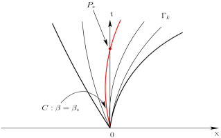
For the QGRP, we shall use the following method to give a second order in time approximation of U𝑈U in t𝑡t-axis. For any point P=(0,Δt)subscript𝑃0Δ𝑡P_{*}=(0,\Delta t) with ΔtΔ𝑡\Delta t being small, to evaluate U(P)𝑈subscript𝑃U(P_{*}), we need to find the initial slope β0subscript𝛽0\beta_{0} of the characteristic curve C𝐶C which emanates from the singularity and goes though Psubscript𝑃P_{*}. See Fig. 5.1. Since for any (x(t),t)C𝑥𝑡𝑡𝐶(x(t),t)\in C,

x(t)=0tλds=0t(λk(0)+Dλkλk(0)s+O(s2))ds,𝑥𝑡superscriptsubscript0𝑡𝜆differential-d𝑠superscriptsubscript0𝑡subscript𝜆𝑘0subscript𝐷subscript𝜆𝑘subscript𝜆𝑘0𝑠𝑂superscript𝑠2differential-d𝑠x(t)=\int_{0}^{t}\lambda\,\mathrm{d}s=\int_{0}^{t}\big{(}\lambda_{k}(0)+D_{\lambda_{k}}\lambda_{k}(0)s+O(s^{2})\big{)}\,\mathrm{d}s, (5.15)

the initial slope β=λk(0)subscript𝛽subscript𝜆𝑘0\beta_{*}=\lambda_{k}(0) can be approximated by solving

β+Dλkλk(β)Δt2=0,subscript𝛽subscript𝐷subscript𝜆𝑘subscript𝜆𝑘subscript𝛽Δ𝑡20\beta_{*}+D_{\lambda_{k}}\lambda_{k}(\beta_{*})\frac{\Delta t}{2}=0, (5.16)

for which, we can use the Newton iteration with initial guess β=0subscript𝛽0\beta_{*}=0.

Having determined βsubscript𝛽\beta_{*}, U(P)𝑈subscript𝑃U(P_{*}) can be evaluated as

U(P)U(β)+DλkU(β)Δt+Dλk2U(β)Δt22.𝑈subscript𝑃𝑈subscript𝛽subscript𝐷subscript𝜆𝑘𝑈subscript𝛽Δ𝑡superscriptsubscript𝐷subscript𝜆𝑘2𝑈subscript𝛽Δsuperscript𝑡22U(P_{*})\approx U(\beta_{*})+D_{\lambda_{k}}U(\beta_{*})\Delta t+D_{\lambda_{k}}^{2}U(\beta_{*})\frac{\Delta t^{2}}{2}. (5.17)
Refer to caption
Figure 5.1: The characteristic curve β=β𝛽subscript𝛽\beta=\beta_{*}, red line.

6 The acoustic approximation

As U=U+subscript𝑈subscript𝑈U_{-}=U_{+} and xP(0)xP+(0+)superscriptsubscript𝑥subscript𝑃superscript0superscriptsubscript𝑥subscript𝑃superscript0\partial_{x}^{\ell}P_{-}(0^{-})\neq\partial_{x}^{\ell}P_{+}(0^{+}), we refer it to as the acoustic case and all waves ΓksubscriptΓ𝑘\Gamma_{k} are acoustic. Fixed λksubscript𝜆𝑘\lambda_{k}, the wave ΓksubscriptΓ𝑘\Gamma_{k} degenerates to a characteristic curve and the states ULsubscript𝑈𝐿U_{L}, URsubscript𝑈𝑅U_{R} on both sides of ΓksubscriptΓ𝑘\Gamma_{k} are the same. In particular, as the initial data has a small jump UU+1much-less-thannormsubscript𝑈subscript𝑈1\|U_{-}-U_{+}\|\ll 1, we adopt the acoustic approximation in the sense that Usubscript𝑈U_{-} and U+subscript𝑈U_{+} are regarded as the same approximately.

Now let us look at the acoustic wave ΓksubscriptΓ𝑘\Gamma_{k}. We use the continuity property of U𝑈U and make differentiation along ΓksubscriptΓ𝑘\Gamma_{k} to obtain DλkUL=DλkURsubscript𝐷subscript𝜆𝑘subscript𝑈𝐿subscript𝐷subscript𝜆𝑘subscript𝑈𝑅D_{\lambda_{k}}U_{L}=D_{\lambda_{k}}U_{R}. Then we proceed to use (3.1) to get

(λkIA)L(xU)L+HL=(λkIA)R(xU)R+HR.subscriptsubscript𝜆𝑘𝐼𝐴𝐿subscriptsubscript𝑥𝑈𝐿subscript𝐻𝐿subscriptsubscript𝜆𝑘𝐼𝐴𝑅subscriptsubscript𝑥𝑈𝑅subscript𝐻𝑅(\lambda_{k}I-A)_{L}(\partial_{x}U)_{L}+H_{L}=(\lambda_{k}I-A)_{R}(\partial_{x}U)_{R}+H_{R}. (6.1)

Note that UL=URsubscript𝑈𝐿subscript𝑈𝑅U_{L}=U_{R} and recall the notation L(k)=(L1,,Lk1,Lk+1,,Lm)Tsuperscript𝐿𝑘superscriptsubscript𝐿1subscript𝐿𝑘1subscript𝐿𝑘1subscript𝐿𝑚𝑇L^{(k)}=(L_{1},\cdots,L_{k-1},L_{k+1},\cdots,L_{m})^{T} in (3.4). Then we find that the (6.1) is equivalent to

L(k)(xU)L=L(k)(xU)R.superscript𝐿𝑘subscriptsubscript𝑥𝑈𝐿superscript𝐿𝑘subscriptsubscript𝑥𝑈𝑅L^{(k)}(\partial_{x}U)_{L}=L^{(k)}(\partial_{x}U)_{R}. (6.2)

Moreover, applying Dλksubscript𝐷subscript𝜆𝑘D_{\lambda_{k}} to (6.2) yields

(λkIΛ(k))L(k)subscript𝜆𝑘𝐼superscriptΛ𝑘superscript𝐿𝑘\displaystyle(\lambda_{k}I-\Lambda^{(k)})L^{(k)} ((x2U)R(x2U)L)=subscriptsuperscriptsubscript𝑥2𝑈𝑅subscriptsuperscriptsubscript𝑥2𝑈𝐿absent\displaystyle\big{(}(\partial_{x}^{2}U)_{R}-(\partial_{x}^{2}U)_{L}\big{)}=
DλkL(k)((xU)L(xU)R)L(k)((xAxU)L(xAxU)R).subscript𝐷subscript𝜆𝑘superscript𝐿𝑘subscriptsubscript𝑥𝑈𝐿subscriptsubscript𝑥𝑈𝑅superscript𝐿𝑘subscriptsubscript𝑥𝐴subscript𝑥𝑈𝐿subscriptsubscript𝑥𝐴subscript𝑥𝑈𝑅\displaystyle D_{\lambda_{k}}L^{(k)}\big{(}(\partial_{x}U)_{L}-(\partial_{x}U)_{R}\big{)}-L^{(k)}\big{(}(\partial_{x}A\partial_{x}U)_{L}-(\partial_{x}A\partial_{x}U)_{R}\big{)}. (6.3)

In addition, if (xU)L=(xU)Rsubscriptsubscript𝑥𝑈𝐿subscriptsubscript𝑥𝑈𝑅(\partial_{x}U)_{L}=(\partial_{x}U)_{R}, then (6) is reduced to

L(k)(x2U)L=L(k)(x2U)R.superscript𝐿𝑘subscriptsuperscriptsubscript𝑥2𝑈𝐿superscript𝐿𝑘subscriptsuperscriptsubscript𝑥2𝑈𝑅L^{(k)}(\partial_{x}^{2}U)_{L}=L^{(k)}(\partial_{x}^{2}U)_{R}. (6.4)

Interestingly, in the course of acoustic approximation, we can obtain xUsubscriptsuperscript𝑥𝑈\partial^{\ell}_{x}U equivalently by solving linear classical Riemann-type problems

{t(xU)+A(U)x(xU)=0,xU(x,0)={xP(0)ifx<0,xP+(0)ifx>0.cases𝑡superscriptsubscript𝑥𝑈𝐴subscript𝑈𝑥superscriptsubscript𝑥𝑈0superscriptsubscript𝑥𝑈𝑥0casessuperscriptsubscript𝑥subscript𝑃0if𝑥0superscriptsubscript𝑥subscript𝑃0if𝑥0\left\{\begin{array}[]{l}\frac{\partial}{\partial t}\left(\partial_{x}^{\ell}U\right)+A(U_{*})\frac{\partial}{\partial x}\left(\partial_{x}^{\ell}U\right)=0,\\[5.69054pt] \partial_{x}^{\ell}U(x,0)=\left\{\begin{array}[]{ll}\partial_{x}^{\ell}P_{-}(0)&\textrm{if}\ x<0,\\ \partial_{x}^{\ell}P_{+}(0)&\textrm{if}\ x>0.\end{array}\right.\end{array}\right. (6.5)

with U=(U+U+)/2subscript𝑈subscript𝑈subscript𝑈2U_{*}=(U_{-}+U_{+})/2. Note that the components of L(k)xUsuperscript𝐿𝑘subscript𝑥𝑈L^{(k)}\partial_{x}U in (6.2) are nothing but the m1𝑚1m-1 generalized Riemann invariants of system (6.5) associated with λksubscript𝜆𝑘\lambda_{k}. We also note that, as indicated by (6.2) or (6.5), the spatial derivatives xUsubscript𝑥𝑈\partial_{x}U are independent of the source term H𝐻H. In addition, if xP(0)xP+(0)subscript𝑥subscript𝑃0subscript𝑥subscript𝑃0\partial_{x}P_{-}(0)\approx\partial_{x}P_{+}(0), from (6.4), we see that x2Usuperscriptsubscript𝑥2𝑈\partial_{x}^{2}U can also be approximated by solving (6.5) with =22\ell=2. In general, we have the following proposition.

Proposition 6.1

For any k1𝑘1k\geq 1, assume that we have xP(0)=xP+(0)superscriptsubscript𝑥subscript𝑃0superscriptsubscript𝑥subscript𝑃0\partial_{x}^{\ell}P_{-}(0)=\partial_{x}^{\ell}P_{+}(0) (0k10𝑘10\leq\ell\leq k-1 with x0Usuperscriptsubscript𝑥0𝑈\partial_{x}^{0}U stands for U𝑈U). Then xkUsuperscriptsubscript𝑥𝑘𝑈\partial_{x}^{k}U are determined by the linear system (6.5) with =k𝑘\ell=k.

Remark 6.1

(i) Since U𝑈U is analytical in the regions Ωj1/2subscriptΩ𝑗12\Omega_{j-1/2} (j=1,,m+1𝑗1𝑚1j=1,\cdots,m+1), the corresponding time derivatives tUsuperscriptsubscript𝑡𝑈\partial_{t}^{\ell}U, 0k0𝑘0\leq\ell\leq k follow from the Cauchy-Kowalewski procedure as illustrated in [22].

(ii) We note here that, under the acoustic assumption in Proposition 6.1, all the approximate DRP solvers proposed in [12, 23, 8] are valid and are actually equivalent to the present acoustic GRP solvers.

As for the resolution of GRP (1.1)-(2.2), if the initial data (2.2) has a jump discontinuity, we can derive the solvers analytically as in Section 5 to calculate the time derivatives of U𝑈U, with possible acoustic approximation for a partial set of waves. This leads to the solver which we label as the LGRP (QGRP) solver. While the jump U+Usubscript𝑈subscript𝑈U_{+}-U_{-} of U𝑈U is very small, we can use (6.5) (or possibly (6)) to calculate the space derivatives approximately. The resulting LGRP (QGRP) solver is labeled as the LGRP1 (QGRP1) solver.

7 An example: The variable area duct flow system

In this section, we will take the system of variable area duct flow as an example to test the GRP solvers in the previous section. The flow system is

tU+A(x)1x[A(x)F(U)]+xG(U)=0,𝑡𝑈𝐴superscript𝑥1𝑥delimited-[]𝐴𝑥𝐹𝑈𝑥𝐺𝑈0\displaystyle\hskip 42.67912pt\frac{\partial}{\partial t}U+A(x)^{-1}\frac{\partial}{\partial x}\big{[}A(x)F(U)\big{]}+\frac{\partial}{\partial x}G(U)=0, (7.6)
U=(ρρuE),F(U)=(ρρu2+p(E+p)u),G(U)=(0p0).formulae-sequence𝑈matrix𝜌𝜌𝑢𝐸formulae-sequence𝐹𝑈matrix𝜌𝜌superscript𝑢2𝑝𝐸𝑝𝑢𝐺𝑈matrix0𝑝0\displaystyle U=\begin{pmatrix}\rho\\ \rho u\\ E\end{pmatrix},\quad F(U)=\begin{pmatrix}\rho\\ \rho u^{2}+p\\ (E+p)u\end{pmatrix},\quad G(U)=\begin{pmatrix}0\\ p\\ 0\end{pmatrix}.

Here, ρ𝜌\rho, u𝑢u, e𝑒e are the density, velocity and internal energy, respectively. p=p(ρ,e)𝑝𝑝𝜌𝑒p=p(\rho,e) is the pressure, E=ρ(e+1/2u2)𝐸𝜌𝑒12superscript𝑢2E=\rho(e+{1}/{2}u^{2}) is the total energy and the function A(x)𝐴𝑥A(x) is the area of the duct. When A(x)=1𝐴𝑥1A(x)=1, the system (7.6) represents the planar compressible Euler equations. We discuss the case of polytropic gases, for which p=(γ1)ρe𝑝𝛾1𝜌𝑒p=(\gamma-1)\rho e, where γ𝛾\gamma is the ratio of specific heats.

7.1 Formulation of the GRP Solvers

In terms of the primitive variables Q=(ρ,u,p)𝑄𝜌𝑢𝑝Q=(\rho,u,p), system (7.6) can be written, for smooth flow, as

Qt+JQx=H,J=(uρ00u1ρ0ρc2u),H=(A(x)A(x)ρu0A(x)A(x)ρc2u).formulae-sequence𝑄𝑡𝐽𝑄𝑥𝐻formulae-sequence𝐽𝑢𝜌00𝑢1𝜌0𝜌superscript𝑐2𝑢𝐻matrixsuperscript𝐴𝑥𝐴𝑥𝜌𝑢0superscript𝐴𝑥𝐴𝑥𝜌superscript𝑐2𝑢\frac{\partial Q}{\partial t}+J\frac{\partial Q}{\partial x}=H,\quad J=\left(\begin{array}[]{ccc}u&\rho&0\\ 0&u&\frac{1}{\rho}\\ 0&\rho c^{2}&u\\ \end{array}\right),\quad H=\begin{pmatrix}-\frac{A^{\prime}(x)}{A(x)}\rho u\\ 0\\ -\frac{A^{\prime}(x)}{A(x)}\rho c^{2}u\end{pmatrix}. (7.7)

Here, c𝑐c is the local speed of sound, given by c2=γpρsuperscript𝑐2𝛾𝑝𝜌c^{2}=\frac{\gamma p}{\rho}.

The system (7.6), or equivalently (7.7), possesses three eigenvalues

λ=uc,λ0=u,λ+=u+c.formulae-sequencesubscript𝜆𝑢𝑐formulae-sequencesubscript𝜆0𝑢subscript𝜆𝑢𝑐\lambda_{-}=u-c,\quad\lambda_{0}=u,\quad\lambda_{+}=u+c.

The three pairs

w=(S,ψ),w0=(u,p),w+=(S,ϕ)formulae-sequencesubscriptw𝑆𝜓formulae-sequencesubscriptw0𝑢𝑝subscriptw𝑆italic-ϕ\textbf{{w}}_{-}=(S,\psi),\quad\textbf{{w}}_{0}=(u,p),\quad\textbf{{w}}_{+}=(S,\phi)

are the generalized Riemann invariants associated with λsubscript𝜆\lambda_{-}, λ0subscript𝜆0\lambda_{0}, λ+subscript𝜆\lambda_{+}. Here, S=pργ𝑆𝑝superscript𝜌𝛾S=p\rho^{-\gamma} is the the entropy, and the two varibles ψ𝜓\psi, ϕitalic-ϕ\phi are

ψ=u+2γ1cϕ=u2γ1c.formulae-sequence𝜓𝑢2𝛾1𝑐italic-ϕ𝑢2𝛾1𝑐\psi=u+\frac{2}{\gamma-1}c\quad\phi=u-\frac{2}{\gamma-1}c.

We now start to resolve the generalized Riemann problem for (7.6) subject to initial data (2.2). Assume that the configuration is as shown in Fig.7.1: a rarefaction wave ΓsubscriptΓ\Gamma_{-} associated with λsubscript𝜆\lambda_{-} moves to the left, a shock wave Γ+subscriptΓ\Gamma_{+} associated with λ+subscript𝜆\lambda_{+} moves to the right. For the variable U𝑈U, let us denote by ULsubscript𝑈𝐿U_{L} and URsubscript𝑈𝑅U_{R} its values on the left-hand side and right-hand side of the three waves, respectively. Similarly, the values of U𝑈U on the two side of Γ0subscriptΓ0\Gamma_{0} are denoted by ULsuperscriptsubscript𝑈𝐿U_{L}^{*} and URsuperscriptsubscript𝑈𝑅U_{R}^{*}, as is illustrated by Fig. 7.1. Similar notations will be applied to other variables. For example, (xU)Lsuperscriptsubscriptsubscript𝑥𝑈𝐿(\partial_{x}U)_{L}^{*} is the value of xUsubscript𝑥𝑈\partial_{x}U on the left-hand side domain of the contact discontinuity.

Refer to caption
Figure 7.1: Typical wave configuration of the variable area duct flow system.

As stated in Section 5, to resolve rarefaction wave associated with λsubscript𝜆\lambda_{-}, we need to use the associated GRI wsubscriptw\textbf{{w}}_{-}. Indeed, in view of Proposition 3.1, we have the following equation for wsubscriptw\textbf{{w}}_{-},

wt+Bwx=H,B=(u01γ1ργ1u+c),H=(0A(x)A(x)cu).formulae-sequencesubscriptw𝑡subscript𝐵subscriptw𝑥subscript𝐻formulae-sequencesubscript𝐵𝑢01𝛾1superscript𝜌𝛾1𝑢𝑐subscript𝐻matrix0superscript𝐴𝑥𝐴𝑥𝑐𝑢\frac{\partial\textbf{{w}}_{-}}{\partial t}+B_{-}\frac{\partial\textbf{{w}}_{-}}{\partial x}=H_{-},\quad B_{-}=\left(\begin{array}[]{cc}u&0\\ -\frac{1}{\gamma-1}\rho^{\gamma-1}&u+c\end{array}\right),\quad H_{-}=\begin{pmatrix}0\\ -\frac{A^{\prime}(x)}{A(x)}cu\end{pmatrix}. (7.8)

By recalling S(0,β)=SL𝑆0𝛽subscript𝑆𝐿S(0,\beta)=S_{L}, ψ(0,β)=ϕL𝜓0𝛽subscriptitalic-ϕ𝐿\psi(0,\beta)=\phi_{L}, λ(0,β)=βsubscript𝜆0𝛽𝛽\lambda_{-}(0,\beta)=\beta in the rarefaction wave fan and using the L(Q)-equations in Proposition 3.2, we can obtain the following proposition. The coefficients A1,,A19subscript𝐴1subscript𝐴19A_{1},\cdots,A_{19}, B1,,B12subscript𝐵1subscript𝐵12B_{1},\cdots,B_{12}, Z1(β)subscript𝑍1𝛽Z_{1}(\beta) and Z2(β)subscript𝑍2𝛽Z_{2}(\beta) are given in A.

Proposition 7.1 (L(Q)-equations: γ3,5/3𝛾353\gamma\neq 3,5/3)

Let ΓsubscriptΓ\Gamma_{-} be the rarefaction wave as in Fig. 7.1. Then for γ5/3,3𝛾533\gamma\neq 5/3,3, we have

DλS(0,β)=A1(ψLβ)γ+1γ1,Dλψ(0,β)=A2(ψLβ)γ+12(γ1)+A3(ψLβ)2γγ1+B1(ψLβ)+B2(ψLβ)2.formulae-sequencesubscript𝐷subscript𝜆𝑆0𝛽subscript𝐴1superscriptsubscript𝜓𝐿𝛽𝛾1𝛾1subscript𝐷subscript𝜆𝜓0𝛽subscript𝐴2superscriptsubscript𝜓𝐿𝛽𝛾12𝛾1subscript𝐴3superscriptsubscript𝜓𝐿𝛽2𝛾𝛾1subscript𝐵1subscript𝜓𝐿𝛽subscript𝐵2superscriptsubscript𝜓𝐿𝛽2\begin{split}&D_{\lambda_{-}}S(0,\beta)=A_{1}(\psi_{L}-\beta)^{\frac{\gamma+1}{\gamma-1}},\\ &D_{\lambda_{-}}\psi(0,\beta)=A_{2}(\psi_{L}-\beta)^{\frac{\gamma+1}{2(\gamma-1)}}+A_{3}(\psi_{L}-\beta)^{\frac{2\gamma}{\gamma-1}}+B_{1}(\psi_{L}-\beta)+B_{2}(\psi_{L}-\beta)^{2}.\end{split} (7.9)

and

Dλ2S(0,β)=[(ψLβL)2(γ+1)γ1DλS(0,βL)+Z1(β)Z1(βL)](ψLβ)2(γ+1)γ1,Dλψ(0,β)=[(ψLβL)γ+1γ1Dλψ(0,βL)+Z2(β)Z2(βL)](ψLβ)γ+1γ1,formulae-sequencesuperscriptsubscript𝐷subscript𝜆2𝑆0𝛽delimited-[]superscriptsubscript𝜓𝐿subscript𝛽𝐿2𝛾1𝛾1subscript𝐷subscript𝜆𝑆0subscript𝛽𝐿subscript𝑍1𝛽subscript𝑍1subscript𝛽𝐿superscriptsubscript𝜓𝐿𝛽2𝛾1𝛾1subscript𝐷subscript𝜆𝜓0𝛽delimited-[]superscriptsubscript𝜓𝐿subscript𝛽𝐿𝛾1𝛾1subscript𝐷subscript𝜆𝜓0subscript𝛽𝐿subscript𝑍2𝛽subscript𝑍2subscript𝛽𝐿superscriptsubscript𝜓𝐿𝛽𝛾1𝛾1\begin{split}&D_{\lambda_{-}}^{2}S(0,\beta)=\big{[}(\psi_{L}-\beta_{L})^{-\frac{2(\gamma+1)}{\gamma-1}}D_{\lambda_{-}}S(0,\beta_{L})+Z_{1}(\beta)-Z_{1}(\beta_{L})\big{]}(\psi_{L}-\beta)^{\frac{2(\gamma+1)}{\gamma-1}},\\ &D_{\lambda_{-}}\psi(0,\beta)=\big{[}(\psi_{L}-\beta_{L})^{-\frac{\gamma+1}{\gamma-1}}D_{\lambda_{-}}\psi(0,\beta_{L})+Z_{2}(\beta)-Z_{2}(\beta_{L})\big{]}(\psi_{L}-\beta)^{\frac{\gamma+1}{\gamma-1}},\end{split} (7.10)

for β[βL,βL]𝛽subscript𝛽𝐿superscriptsubscript𝛽𝐿\beta\in[\beta_{L},\beta_{L}^{*}].

Remark 7.1

(i) For the cases of γ=5/3,3𝛾533\gamma=5/3,3, the L-equations of wsubscriptw\textbf{{w}}_{-} are given in A. The corresponding Q-equations are omitted here. Besides, the formulae for xS(0,β)subscript𝑥𝑆0𝛽\partial_{x}S(0,\beta) and xΨ(0,β)subscript𝑥Ψ0𝛽\partial_{x}\Psi(0,\beta), which can be obtained by integrating (3.21) directly, are also omitted here.

(ii) For γ5/3,3𝛾533\gamma\neq 5/3,3, the differential relation in the rarefaction wave fan associated with λsubscript𝜆\lambda_{-}

Dλϕ=1γ(γ1)cSDλS+A(x)A(x)cusubscript𝐷subscript𝜆italic-ϕ1𝛾𝛾1𝑐𝑆subscript𝐷subscript𝜆𝑆superscript𝐴𝑥𝐴𝑥𝑐𝑢\displaystyle D_{\lambda_{-}}\phi=-\frac{1}{\gamma(\gamma-1)}\frac{c}{S}D_{\lambda_{-}}S+\frac{A^{\prime}(x)}{A(x)}cu (7.11)

leads to

Dλϕ=A4(ψLβ)2γγ1+B3(ψLβ)+B4(ψLβ)2.subscript𝐷subscript𝜆italic-ϕsubscript𝐴4superscriptsubscript𝜓𝐿𝛽2𝛾𝛾1subscript𝐵3subscript𝜓𝐿𝛽subscript𝐵4superscriptsubscript𝜓𝐿𝛽2\displaystyle D_{\lambda_{-}}\phi=A_{4}(\psi_{L}-\beta)^{\frac{2\gamma}{\gamma-1}}+B_{3}(\psi_{L}-\beta)+B_{4}(\psi_{L}-\beta)^{2}. (7.12)

By noticing λ=3γ4ψ+1+γ4ϕsubscript𝜆3𝛾4𝜓1𝛾4italic-ϕ\lambda_{-}=\frac{3-\gamma}{4}\psi+\frac{1+\gamma}{4}\phi,

we have

β(Dλλ)=A7(ψLβ)γ+12(γ1)+A8(ψLβ)2γγ1+B7(ψLβ)+B8(ψLβ)2.𝛽subscript𝐷subscript𝜆subscript𝜆subscript𝐴7superscriptsubscript𝜓𝐿𝛽𝛾12𝛾1subscript𝐴8superscriptsubscript𝜓𝐿𝛽2𝛾𝛾1subscript𝐵7subscript𝜓𝐿𝛽subscript𝐵8superscriptsubscript𝜓𝐿𝛽2\displaystyle\frac{\partial}{\partial\beta}(D_{\lambda_{-}}\lambda_{-})=A_{7}(\psi_{L}-\beta)^{\frac{\gamma+1}{2(\gamma-1)}}+A_{8}(\psi_{L}-\beta)^{\frac{2\gamma}{\gamma-1}}+B_{7}(\psi_{L}-\beta)+B_{8}(\psi_{L}-\beta)^{2}. (7.13)

Moreover, Dλ2ϕsuperscriptsubscript𝐷subscript𝜆2italic-ϕD_{\lambda_{-}}^{2}\phi can be determined by

Dλ2ϕ=1γ(γ1)(cSDλ2S+Dλ(cS)DλS)+Dλ(A(x)A(x)cu),superscriptsubscript𝐷subscript𝜆2italic-ϕ1𝛾𝛾1𝑐𝑆superscriptsubscript𝐷subscript𝜆2𝑆subscript𝐷subscript𝜆𝑐𝑆subscript𝐷subscript𝜆𝑆subscript𝐷subscript𝜆superscript𝐴𝑥𝐴𝑥𝑐𝑢\displaystyle D_{\lambda_{-}}^{2}\phi=-\frac{1}{\gamma(\gamma-1)}\left(\frac{c}{S}D_{\lambda_{-}}^{2}S+D_{\lambda_{-}}\left(\frac{c}{S}\right)D_{\lambda_{-}}S\right)+D_{\lambda_{-}}\left(\frac{A^{\prime}(x)}{A(x)}cu\right), (7.14)

which follows from (7.11). The above formulas will be used to resolve the sonic case. See Proposition 7.4.

We also note that, in order to resolve the contact discontinuity wave Γ0subscriptΓ0\Gamma_{0}, the following equation of w0subscriptw0\textbf{{w}}_{0} will be used,

w0t+B0w0x=H0,B0=(u1ρρc2u),H0=(0A(x)A(x)ρc2u).formulae-sequencesubscriptw0𝑡subscript𝐵0subscriptw0𝑥subscript𝐻0formulae-sequencesubscript𝐵0𝑢1𝜌𝜌superscript𝑐2𝑢subscript𝐻0matrix0superscript𝐴𝑥𝐴𝑥𝜌superscript𝑐2𝑢\frac{\partial\textbf{{w}}_{0}}{\partial t}+B_{0}\frac{\partial\textbf{{w}}_{0}}{\partial x}=H_{0},\quad B_{0}=\left(\begin{array}[]{cc}u&\frac{1}{\rho}\\ \rho c^{2}&u\end{array}\right),\quad H_{0}=\begin{pmatrix}0\\ -\frac{A^{\prime}(x)}{A(x)}\rho c^{2}u\end{pmatrix}. (7.15)

Now let us present the LGRP solver for problem (7.6)-(2.2) in the following proposition, corresponding to the wave configuration in Fig. 7.1.

Proposition 7.2 (Linear GRP)

Assume a typical wave configuration for the generalized Riemann problem of (7.6) and (2.2) as shown in Fig.7.1. Then (xQ)Lsuperscriptsubscriptsubscript𝑥𝑄𝐿(\partial_{x}Q)_{L}^{*} and (xQ)Rsuperscriptsubscriptsubscript𝑥𝑄𝑅(\partial_{x}Q)_{R}^{*} are determined by the set of linear equations

[(λIB)Qw]L(xQ)L=Dλw(UL)H(UL),(λ0IB0)L(xw0)L(λ0IB0)R(xw0)R=H0(UL)+H0(UR),[(QFσQU)(σIJ)]R(xQ)RDσσ(URUR)=[(QFσQU)(σIJ)]L(xQ)R[(QFσQU)H]R+[(QFσQU)H]R.formulae-sequencesuperscriptsubscriptdelimited-[]subscript𝜆𝐼subscript𝐵subscript𝑄subscriptw𝐿superscriptsubscriptsubscript𝑥𝑄𝐿subscript𝐷subscript𝜆subscriptwsuperscriptsubscript𝑈𝐿subscript𝐻superscriptsubscript𝑈𝐿formulae-sequencesuperscriptsubscriptsubscript𝜆0𝐼subscript𝐵0𝐿superscriptsubscriptsubscript𝑥subscriptw0𝐿superscriptsubscriptsubscript𝜆0𝐼subscript𝐵0𝑅superscriptsubscriptsubscript𝑥subscriptw0𝑅subscript𝐻0superscriptsubscript𝑈𝐿subscript𝐻0superscriptsubscript𝑈𝑅superscriptsubscriptdelimited-[]subscript𝑄𝐹𝜎subscript𝑄𝑈𝜎𝐼𝐽𝑅superscriptsubscriptsubscript𝑥𝑄𝑅subscript𝐷𝜎𝜎superscriptsubscript𝑈𝑅subscript𝑈𝑅superscriptsubscriptdelimited-[]subscript𝑄𝐹𝜎subscript𝑄𝑈𝜎𝐼𝐽𝐿subscriptsubscript𝑥𝑄𝑅superscriptsubscriptdelimited-[]subscript𝑄𝐹𝜎subscript𝑄𝑈𝐻𝑅subscriptdelimited-[]subscript𝑄𝐹𝜎subscript𝑄𝑈𝐻𝑅\begin{split}&[(\lambda_{-}I-B_{-})\nabla_{Q}\textbf{{w}}_{-}]_{L}^{*}(\partial_{x}Q)_{L}^{*}=D_{\lambda_{-}}\textbf{{w}}_{-}(U_{L}^{*})-H_{-}(U_{L}^{*}),\\[5.69054pt] &(\lambda_{0}I-B_{0})_{L}^{*}(\partial_{x}\textbf{{w}}_{0})_{L}^{*}-(\lambda_{0}I-B_{0})_{R}^{*}(\partial_{x}\textbf{{w}}_{0})_{R}^{*}=-H_{0}(U_{L}^{*})+H_{0}(U_{R}^{*}),\\[5.69054pt] &[(\nabla_{Q}F-\sigma\nabla_{Q}U)(\sigma I-J)]_{R}^{*}(\partial_{x}Q)_{R}^{*}-D_{\sigma}\sigma(U_{R}^{*}-U_{R})=\\[5.69054pt] &[(\nabla_{Q}F-\sigma\nabla_{Q}U)(\sigma I-J)]_{L}^{*}(\partial_{x}Q)_{R}-[(\nabla_{Q}F-\sigma\nabla_{Q}U)H]_{R}^{*}+[(\nabla_{Q}F-\sigma\nabla_{Q}U)H]_{R}.\end{split} (7.16)

Here, Dλw(UL)subscript𝐷subscript𝜆subscriptwsuperscriptsubscript𝑈𝐿D_{\lambda_{-}}\textbf{{w}}_{-}(U_{L}^{*}) is determined by (7.9), σ𝜎\sigma is the speed of the shock associated with λ+=u+csubscript𝜆𝑢𝑐\lambda_{+}=u+c.

Moreover, for the sonic case where the t𝑡t-axis is located in the rarefaction, the tQsubscript𝑡𝑄\partial_{t}Q at t𝑡t-axis (β=0𝛽0\beta=0) are determined by

[(λIB)Qw](tQ)=DλwH,tu+1ρctp=A(x)A(x)cu,formulae-sequencedelimited-[]subscript𝜆𝐼subscript𝐵subscript𝑄subscriptwsubscript𝑡𝑄subscript𝐷subscript𝜆subscriptwsubscript𝐻subscript𝑡𝑢1𝜌𝑐subscript𝑡𝑝superscript𝐴𝑥𝐴𝑥𝑐𝑢\begin{split}&[(\lambda_{-}I-B_{-})\nabla_{Q}\textbf{{w}}_{-}](\partial_{t}Q)=D_{\lambda_{-}}\textbf{{w}}_{-}-H_{-},\\[5.69054pt] &\partial_{t}u+\frac{1}{\rho c}\partial_{t}p=\frac{A^{\prime}(x)}{A(x)}cu,\end{split} (7.17)

where the U𝑈U in the coefficients takes value at t𝑡t-axis where λ=0subscript𝜆0\lambda_{-}=0.

Proof. The linear system (7.16) for (xU)Lsuperscriptsubscriptsuperscriptsubscript𝑥𝑈𝐿(\partial_{x}^{*}U)_{L}^{*} and (xU)Rsuperscriptsubscriptsuperscriptsubscript𝑥𝑈𝑅(\partial_{x}^{*}U)_{R}^{*} can be obtained by combining (7.9), (4.1) and (4.5) with l=1𝑙1l=1 and using the following expressions

Dλ(w(U))=(λIB)QwxQ+H,subscript𝐷subscript𝜆subscriptw𝑈subscript𝜆𝐼subscript𝐵subscript𝑄subscriptwsubscript𝑥𝑄subscript𝐻\displaystyle D_{\lambda_{-}}\left(\textbf{{w}}_{-}(U)\right)=(\lambda_{-}I-B_{-})\nabla_{Q}\textbf{{w}}_{-}\partial_{x}Q+H_{-},
Dλ0(w0(U))=(λ0IB0)xw0+H0,subscript𝐷subscript𝜆0subscriptw0𝑈subscript𝜆0𝐼subscript𝐵0subscript𝑥subscriptw0subscript𝐻0\displaystyle D_{\lambda_{0}}\left(\textbf{{w}}_{0}(U)\right)=(\lambda_{0}I-B_{0})\partial_{x}\textbf{{w}}_{0}+H_{0},
Dσ[(QFσQU)]=(QFσQU)[(σIJ)(xQ)+H]Dσ2σU.subscript𝐷𝜎delimited-[]subscript𝑄𝐹𝜎subscript𝑄𝑈subscript𝑄𝐹𝜎subscript𝑄𝑈delimited-[]𝜎𝐼𝐽subscript𝑥𝑄𝐻superscriptsubscript𝐷𝜎2𝜎𝑈\displaystyle D_{\sigma}[(\nabla_{Q}F-\sigma\nabla_{Q}U)]=(\nabla_{Q}F-\sigma\nabla_{Q}U)[(\sigma I-J)(\partial_{x}Q)+H]-D_{\sigma}^{2}\sigma U.

To resolve the sonic case, we shall use the differential relation along the λsubscript𝜆\lambda_{-} characteristic curve:

Dλu+1ρcDλp=A(x)A(x)cu,subscript𝐷subscript𝜆𝑢1𝜌𝑐subscript𝐷subscript𝜆𝑝superscript𝐴𝑥𝐴𝑥𝑐𝑢D_{\lambda_{-}}u+\frac{1}{\rho c}D_{\lambda_{-}}p=\frac{A^{\prime}(x)}{A(x)}cu, (7.18)

which is equivalent to (7.11). (7.17) follows from (7.9) and (7.18) by setting λ=0subscript𝜆0\lambda_{-}=0. MM \square

.

The QGRP solver for the nonsonic case and sonic case are presented in the following two propositions, respectively.

Proposition 7.3 (Quadratic GRP: Nonsonic case)

Assume a typical wave configuration for the generalized Riemann problem of (7.6) and (2.2) as shown in Fig. 7.1. Then (x2Q)Lsuperscriptsubscriptsuperscriptsubscript𝑥2𝑄𝐿(\partial_{x}^{2}Q)_{L}^{*} and (x2Q)Rsuperscriptsubscriptsuperscriptsubscript𝑥2𝑄𝑅(\partial_{x}^{2}Q)_{R}^{*} are determined by the set of linear equations

Mr(UL)(x2Q)L=Dλ2w(UL)Br(UL,(xU)L)Mc(UL)(x2w0)LMc(UR)(x2w0)R=Bc(UL,(xU)L)+Bc(UR,(xU)R),Ms(UR,σ)(x2Q)RDσ2σ(URUR)=Bs(UR,(xU)R,σ,Dσσ)+Ms(UR,σ)(x2Q)R+Bs(UR,(xU)R,σ,Dσσ).formulae-sequencesubscript𝑀𝑟superscriptsubscript𝑈𝐿superscriptsubscriptsuperscriptsubscript𝑥2𝑄𝐿superscriptsubscript𝐷subscript𝜆2subscriptwsuperscriptsubscript𝑈𝐿subscript𝐵𝑟superscriptsubscript𝑈𝐿superscriptsubscriptsubscript𝑥𝑈𝐿subscript𝑀𝑐superscriptsubscript𝑈𝐿superscriptsubscriptsuperscriptsubscript𝑥2subscriptw0𝐿subscript𝑀𝑐superscriptsubscript𝑈𝑅superscriptsubscriptsuperscriptsubscript𝑥2subscriptw0𝑅subscript𝐵𝑐superscriptsubscript𝑈𝐿superscriptsubscriptsubscript𝑥𝑈𝐿subscript𝐵𝑐superscriptsubscript𝑈𝑅superscriptsubscriptsubscript𝑥𝑈𝑅subscript𝑀𝑠superscriptsubscript𝑈𝑅𝜎superscriptsubscriptsuperscriptsubscript𝑥2𝑄𝑅superscriptsubscript𝐷𝜎2𝜎superscriptsubscript𝑈𝑅subscript𝑈𝑅subscript𝐵𝑠superscriptsubscript𝑈𝑅superscriptsubscriptsubscript𝑥𝑈𝑅𝜎subscript𝐷𝜎𝜎subscript𝑀𝑠subscript𝑈𝑅𝜎subscriptsuperscriptsubscript𝑥2𝑄𝑅subscript𝐵𝑠subscript𝑈𝑅subscriptsubscript𝑥𝑈𝑅𝜎subscript𝐷𝜎𝜎\begin{split}&M_{r}(U_{L}^{*})(\partial_{x}^{2}Q)_{L}^{*}=D_{\lambda_{-}}^{2}\textbf{{w}}_{-}(U_{L}^{*})-B_{r}(U_{L}^{*},(\partial_{x}U)_{L}^{*})\\[5.69054pt] &M_{c}(U_{L}^{*})(\partial_{x}^{2}\textbf{{w}}_{0})_{L}^{*}-M_{c}(U_{R}^{*})(\partial_{x}^{2}\textbf{{w}}_{0})_{R}^{*}=-B_{c}\big{(}U_{L}^{*},(\partial_{x}U)_{L}^{*}\big{)}+B_{c}\big{(}U_{R}^{*},(\partial_{x}U)_{R}^{*}\big{)},\\[5.69054pt] &M_{s}(U_{R}^{*},\sigma)(\partial_{x}^{2}Q)_{R}^{*}-D_{\sigma}^{2}\sigma(U_{R}^{*}-U_{R})=-B_{s}\big{(}U_{R}^{*},(\partial_{x}U)_{R}^{*},\sigma,D_{\sigma}\sigma\big{)}\\ &\hskip 128.0374pt+M_{s}(U_{R},\sigma)(\partial_{x}^{2}Q)_{R}+B_{s}\big{(}U_{R},(\partial_{x}U)_{R},\sigma,D_{\sigma}\sigma\big{)}.\end{split} (7.19)

Here, Dλ2w(UL)superscriptsubscript𝐷subscript𝜆2subscriptwsuperscriptsubscript𝑈𝐿D_{\lambda_{-}}^{2}\textbf{{w}}_{-}(U_{L}^{*}) is determined by (7.10), σ𝜎\sigma is the speed of the shock associated with λ+=u+csubscript𝜆𝑢𝑐\lambda_{+}=u+c,

Mr(U)=(λIB)2Qw,subscript𝑀𝑟𝑈superscriptsubscript𝜆𝐼subscript𝐵2subscript𝑄subscriptw\displaystyle M_{r}(U)=(\lambda_{-}I-B_{-})^{2}\nabla_{Q}\textbf{{w}}_{-},
Br(U,xU)=[Dλ(λIB)(λIB)xB]xwsubscript𝐵𝑟𝑈subscript𝑥𝑈delimited-[]subscript𝐷subscript𝜆subscript𝜆𝐼subscript𝐵subscript𝜆𝐼subscript𝐵subscript𝑥subscript𝐵subscript𝑥subscriptw\displaystyle B_{r}(U,\partial_{x}U)=[D_{\lambda_{-}}(\lambda_{-}I-B_{-})-(\lambda_{-}I-B_{-})\partial_{x}B_{-}]\partial_{x}\textbf{{w}}_{-}
+(λIB)2x(Qw)xQ+(λIB)xH+DκH,superscriptsubscript𝜆𝐼subscript𝐵2subscript𝑥subscript𝑄subscriptwsubscript𝑥𝑄subscript𝜆𝐼subscript𝐵subscript𝑥subscript𝐻subscript𝐷subscript𝜅subscript𝐻\displaystyle\hskip 85.35826pt+(\lambda_{-}I-B_{-})^{2}\partial_{x}(\nabla_{Q}\textbf{{w}}_{-})\partial_{x}Q+(\lambda_{-}I-B_{-})\partial_{x}H_{-}+D_{\kappa_{-}}H_{-},
Mc(U)=(λ0IB0)2,subscript𝑀𝑐𝑈superscriptsubscript𝜆0𝐼subscript𝐵02\displaystyle M_{c}(U)=(\lambda_{0}I-B_{0})^{2},
Bc(U,xU)=Du(λ0IB0)xw0(λ0IB0)xB0xw0+(λ0IB0)xH0+Dλ0H0,subscript𝐵𝑐𝑈subscript𝑥𝑈subscript𝐷𝑢subscript𝜆0𝐼subscript𝐵0subscript𝑥subscriptw0subscript𝜆0𝐼subscript𝐵0subscript𝑥subscript𝐵0subscript𝑥subscriptw0subscript𝜆0𝐼subscript𝐵0subscript𝑥subscript𝐻0subscript𝐷subscript𝜆0subscript𝐻0\displaystyle B_{c}(U,\partial_{x}U)=D_{u}(\lambda_{0}I-B_{0})\partial_{x}\textbf{{w}}_{0}-(\lambda_{0}I-B_{0})\partial_{x}B_{0}\partial_{x}\textbf{{w}}_{0}+(\lambda_{0}I-B_{0})\partial_{x}H_{0}+D_{\lambda_{0}}H_{0},
Ms(U,σ)=(QFσQU)(σIJ)2,subscript𝑀𝑠𝑈𝜎subscript𝑄𝐹𝜎subscript𝑄𝑈superscript𝜎𝐼𝐽2\displaystyle M_{s}(U,\sigma)=(\nabla_{Q}F-\sigma\nabla_{Q}U)(\sigma I-J)^{2},
Bs(U,xU,σ,Dσσ)=(Dσ(QF)2DσσQUσDσ(QU))DσQsubscript𝐵𝑠𝑈subscript𝑥𝑈𝜎subscript𝐷𝜎𝜎subscript𝐷𝜎subscript𝑄𝐹2subscript𝐷𝜎𝜎subscript𝑄𝑈𝜎subscript𝐷𝜎subscript𝑄𝑈subscript𝐷𝜎𝑄\displaystyle B_{s}(U,\partial_{x}U,\sigma,D_{\sigma}\sigma)=(D_{\sigma}(\nabla_{Q}F)-2D_{\sigma}\sigma\nabla_{Q}U-\sigma D_{\sigma}(\nabla_{Q}U))D_{\sigma}Q
+(QFσQU)[Dσ(σIJ)(σIJ)xJ]xQsubscript𝑄𝐹𝜎subscript𝑄𝑈delimited-[]subscript𝐷𝜎𝜎𝐼𝐽𝜎𝐼𝐽subscript𝑥𝐽subscript𝑥𝑄\displaystyle\hskip 128.0374pt+(\nabla_{Q}F-\sigma\nabla_{Q}U)[D_{\sigma}(\sigma I-J)-(\sigma I-J)\partial_{x}J]\partial_{x}Q
+(QFσQU)[(σIJ)xH+DσH].subscript𝑄𝐹𝜎subscript𝑄𝑈delimited-[]𝜎𝐼𝐽subscript𝑥𝐻subscript𝐷𝜎𝐻\displaystyle\hskip 128.0374pt+(\nabla_{Q}F-\sigma\nabla_{Q}U)[(\sigma I-J)\partial_{x}H+D_{\sigma}H].

Proof. This proposition can be proved by combining (7.10), (4.1) and (4.5) with l=2𝑙2l=2 and using the following expressions

Dλ2(w(U))=Mr(U)x2Q+Br(U,xU),superscriptsubscript𝐷subscript𝜆2subscriptw𝑈subscript𝑀𝑟𝑈superscriptsubscript𝑥2𝑄subscript𝐵𝑟𝑈subscript𝑥𝑈\displaystyle D_{\lambda_{-}}^{2}\left(\textbf{{w}}_{-}(U)\right)=M_{r}(U)\partial_{x}^{2}Q+B_{r}(U,\partial_{x}U),
Dλ02(w0(U))=Mc(U)x2w0+Bc(U,xU),superscriptsubscript𝐷subscript𝜆02subscriptw0𝑈subscript𝑀𝑐𝑈superscriptsubscript𝑥2subscriptw0subscript𝐵𝑐𝑈subscript𝑥𝑈\displaystyle D_{\lambda_{0}}^{2}\left(\textbf{{w}}_{0}(U)\right)=M_{c}(U)\partial_{x}^{2}\textbf{{w}}_{0}+B_{c}(U,\partial_{x}U),

and

Dσ2(F(U)σU)=Ms(U,σ)x2QDσ2σU+Bs(U,xU,σ,Dσσ).superscriptsubscript𝐷𝜎2𝐹𝑈𝜎𝑈subscript𝑀𝑠𝑈𝜎superscriptsubscript𝑥2𝑄superscriptsubscript𝐷𝜎2𝜎𝑈subscript𝐵𝑠𝑈subscript𝑥𝑈𝜎subscript𝐷𝜎𝜎\displaystyle D_{\sigma}^{2}\big{(}F(U)-\sigma U\big{)}=M_{s}(U,\sigma)\partial_{x}^{2}Q-D_{\sigma}^{2}\sigma U+B_{s}(U,\partial_{x}U,\sigma,D_{\sigma}\sigma).

MM \square

.

Proposition 7.4 (Quadratic GRP: Sonic case)

Assume that the t𝑡t-axis is located inside the rarefaction wave associated with λsubscript𝜆\lambda_{-}. Denoting by Φ=(S,ϕ,ψ)Φ𝑆italic-ϕ𝜓\Phi=(S,\phi,\psi), then for any point P=(0,Δt)subscript𝑃0Δ𝑡P_{*}=(0,\Delta t) with ΔtΔ𝑡\Delta t being small, we have

Φ(P)=Φ(0)+DλΦ(β)Δt+Dλ2Φ(β)Δt22+O(Δt3),Φsubscript𝑃Φ0subscript𝐷subscript𝜆Φsubscript𝛽Δ𝑡superscriptsubscript𝐷subscript𝜆2Φsubscript𝛽Δsuperscript𝑡22𝑂Δsuperscript𝑡3\Phi(P_{*})=\Phi(0)+D_{\lambda_{-}}\Phi(\beta_{*})\Delta t+D_{\lambda_{-}}^{2}\Phi(\beta_{*})\frac{\Delta t^{2}}{2}+O(\Delta t^{3}), (7.20)

where βsubscript𝛽\beta_{*} is the root of

β+Dλλ(β)Δt2=0,𝛽subscript𝐷subscript𝜆subscript𝜆𝛽Δ𝑡20\beta+D_{\lambda_{-}}\lambda_{-}(\beta)\frac{\Delta t}{2}=0, (7.21)

and DλΦsuperscriptsubscript𝐷subscript𝜆ΦD_{\lambda_{-}}^{\ell}\Phi, =1,212\ell=1,2 are determined by (7.9)-(7.14).

The other wave configurations can be treated similarly. In particular, if a λ+subscript𝜆\lambda_{+}-rarefaction wave is involved, in order to get the linear equation for (x2Q)Rsuperscriptsubscriptsuperscriptsubscript𝑥2𝑄𝑅(\partial_{x}^{2}Q)_{R}^{*} analogous to the first equation of (7.19), it requires one to derive the L(Q)-equation for w+subscriptw\textbf{{w}}_{+}. However, a better choice for us is to use the following property of system (7.6): (7.6) holds true under the transformation 𝒯:(ρ,u,p,A)(x,t)(ρ,u,p,A)(x,t):𝒯𝜌𝑢𝑝𝐴𝑥𝑡𝜌𝑢𝑝𝐴𝑥𝑡\mathscr{T}:(\rho,u,p,A)(x,t)\rightarrow(\rho,-u,p,A)(-x,t). In fact, if we denote by Q~=𝒯(Q)~𝑄𝒯𝑄\tilde{Q}=\mathscr{T}(Q), then U~L=𝒯(UR)superscriptsubscript~𝑈𝐿𝒯superscriptsubscript𝑈𝑅\tilde{U}_{L}^{*}=\mathscr{T}(U_{R}^{*}), U~L=𝒯(UR)superscriptsubscript~𝑈𝐿𝒯superscriptsubscript𝑈𝑅\tilde{U}_{L}^{*}=\mathscr{T}(U_{R}^{*}), λ(U~R)=λ+(UL)subscript𝜆superscriptsubscript~𝑈𝑅subscript𝜆superscriptsubscript𝑈𝐿\lambda_{-}(\tilde{U}_{R}^{*})=\lambda_{+}(U_{L}^{*}). By expressing Dλ2w(β)superscriptsubscript𝐷subscript𝜆2subscriptw𝛽D_{\lambda_{-}}^{2}\textbf{{w}}_{-}(\beta) as a function of UL,(xU)L,(x2U)L,A(x),A′′(x)subscript𝑈𝐿subscriptsubscript𝑥𝑈𝐿subscriptsuperscriptsubscript𝑥2𝑈𝐿superscript𝐴𝑥superscript𝐴′′𝑥U_{L},(\partial_{x}U)_{L},(\partial_{x}^{2}U)_{L},A^{\prime}(x),A^{\prime\prime}(x) and β𝛽\beta: Dλ2w(β)=𝒲(UL,(xU)L,(x2U)L,A(x),A′′(x),β)superscriptsubscript𝐷subscript𝜆2subscriptw𝛽𝒲subscript𝑈𝐿subscriptsubscript𝑥𝑈𝐿subscriptsuperscriptsubscript𝑥2𝑈𝐿superscript𝐴𝑥superscript𝐴′′𝑥𝛽D_{\lambda_{-}}^{2}\textbf{{w}}_{-}(\beta)=\mathscr{W}\big{(}U_{L},(\partial_{x}U)_{L},(\partial_{x}^{2}U)_{L},A^{\prime}(x),A^{\prime\prime}(x),\beta\big{)}, we have

Mr(U~L,A(x),A′′(x))(x2Q~)L=subscript𝑀𝑟superscriptsubscript~𝑈𝐿superscript𝐴𝑥superscript𝐴′′𝑥superscriptsubscriptsuperscriptsubscript𝑥2~𝑄𝐿absent\displaystyle M_{r}(\tilde{U}_{L}^{*},-A^{\prime}(x),A^{\prime\prime}(x))(\partial_{x}^{2}\tilde{Q})_{L}^{*}= 𝒲(U~L,xU~L,(x2U~)L,A(x),A′′(x),λ(U~L))𝒲subscript~𝑈𝐿subscript𝑥subscript~𝑈𝐿subscriptsuperscriptsubscript𝑥2~𝑈𝐿superscript𝐴𝑥superscript𝐴′′𝑥subscript𝜆superscriptsubscript~𝑈𝐿\displaystyle\mathscr{W}\big{(}\tilde{U}_{L},\partial_{x}\tilde{U}_{L},(\partial_{x}^{2}\tilde{U})_{L},-A^{\prime}(x),A^{\prime\prime}(x),\lambda_{-}(\tilde{U}_{L}^{*})\big{)}
Br(U~L,(xU~)L,A(x),A′′(x)).subscript𝐵𝑟superscriptsubscript~𝑈𝐿superscriptsubscriptsubscript𝑥~𝑈𝐿superscript𝐴𝑥superscript𝐴′′𝑥\displaystyle\quad-B_{r}\big{(}\tilde{U}_{L}^{*},(\partial_{x}\tilde{U})_{L}^{*},-A^{\prime}(x),A^{\prime\prime}(x)\big{)}. (7.22)

Noting that (x2Q)R=((x2ρ~)L,(x2u~)L,(x2p~)L)superscriptsubscriptsuperscriptsubscript𝑥2𝑄𝑅superscriptsubscriptsuperscriptsubscript𝑥2~𝜌𝐿superscriptsubscriptsuperscriptsubscript𝑥2~𝑢𝐿superscriptsubscriptsuperscriptsubscript𝑥2~𝑝𝐿(\partial_{x}^{2}{Q})_{R}^{*}=((\partial_{x}^{2}\tilde{\rho})_{L}^{*},-(\partial_{x}^{2}\tilde{u})_{L}^{*},(\partial_{x}^{2}\tilde{p})_{L}^{*}), (7.1) is indeed the derived linear equation for (x2Q)Rsuperscriptsubscriptsuperscriptsubscript𝑥2𝑄𝑅(\partial_{x}^{2}Q)_{R}^{*}. The sonic case corresponding to the λ+subscript𝜆\lambda_{+}-rarefaction wave can be resolved using the same technique.

7.2 Tests for the GRP solvers

In this section we assess the performance of the GRP solvers for the compressible Euler equations system, i.e. (7.6) with A(x)=1𝐴𝑥1A(x)=1. The aim is to show, via several test problems, the accuracy and behavior of the present solvers. As tests, we use the generalized Riemann problems proposed by [8] and construct new ones with large jumps in pressure. The first test has no jump discontinuities in the state variables but admits discontinuities in derivatives at the interface. The more demanding test problems are constructed from the first one, by adding a discontinuity in pressure. Six new cases are thus generated by varying the strength of the initial pressure jump Δp=(pLpR)/pRΔ𝑝subscript𝑝𝐿subscript𝑝𝑅subscript𝑝𝑅\Delta p=(p_{L}-p_{R})/p_{R} at the interface, namely Δp=10kΔ𝑝superscript10𝑘\Delta p=10^{k}, k=2,,3𝑘23k=-2,\cdots,3. The last test problem for the sonic case are constructed by adding Δu=28Δ𝑢28\Delta u=28 to the initial flow velocity of the test case corresponding to Δp=100Δ𝑝100\Delta p=100.

In [8], the authors test the first five problems using three type of DRP solvers with only partial success. Since no exact solutions are known, the reference solutions are obtained numerically, by solving the test problems on very fine mesh on the interval [1,1]×[0,t0]110subscript𝑡0[-1,1]\times[0,t_{0}] of (x,t)𝑥𝑡(x,t). To do this, the authors of [8, 15] suggest using the Random Choice Method or Weighted Average Flux method to avoid the large nonphysical oscillations of early time solution. To this aspect, a detailed description can be found in [8, 15], which is beyond the scope of this work. Here, our numerical reference solutions are obtained simply by using the Godunov flux in the context of finite volume method and then correcting their values on the early time interval [0,t0/20]0subscript𝑡020[0,t_{0}/20] using an interpolation method. Such a measure does not affect our accuracy tests.

For each of these tests, we will compare the GRP solver based solution at the interface x=0𝑥0x=0, as a function of time determined by (2.5), with the reference numerical solution. As will be shown, the present GRP solvers is truly accurate, having the expected accuracy not only for all the test cases in [8], but also for cases with much larger initial jump in state variables.

7.2.1 Acoustic case with continuous state and jump in derivatives

This test corresponds to the following initial condition

ρL(x,0)=1+0.56431x+2.62896x2,uL(x,0)=0.031251.024x+1.92x2,pL(x,0)=100.216x+1.08x2,ρR(x,0)=1+2.04204x,uR(x,0)=0.031250.25x+0.75x2,pR(x,0)=10,formulae-sequencesubscript𝜌𝐿𝑥010.56431𝑥2.62896superscript𝑥2formulae-sequencesubscript𝑢𝐿𝑥00.031251.024𝑥1.92superscript𝑥2formulae-sequencesubscript𝑝𝐿𝑥0100.216𝑥1.08superscript𝑥2formulae-sequencesubscript𝜌𝑅𝑥012.04204𝑥formulae-sequencesubscript𝑢𝑅𝑥00.031250.25𝑥0.75superscript𝑥2subscript𝑝𝑅𝑥010\begin{split}&\rho_{L}(x,0)=1+0.56431x+2.62896x^{2},\\[5.69054pt] &u_{L}(x,0)=0.03125-1.024x+1.92x^{2},\\[5.69054pt] &p_{L}(x,0)=10-0.216x+1.08x^{2},\\[5.69054pt] &\rho_{R}(x,0)=1+2.04204x,\\[5.69054pt] &u_{R}(x,0)=0.03125-0.25x+0.75x^{2},\\[5.69054pt] &p_{R}(x,0)=10,\end{split} (7.23)

which is indeed the initial conditions used as Test 2 in [8] with slight modification, keeping only the same leading terms up to second order at x=0𝑥0x=0. The initial condition (7.23) has a continuous state but with discontinuous derivatives at x=0𝑥0x=0. The solution for this problem contains a left-going and a right-going acoustic waves. The t𝑡t-axis is located in the intermediate region of the two acoustic waves. This test aims at testing the accuracy of the acoustic GRP solvers. Fig. 7.2 shows the solution of LGRP1 solver and QGRP1 solver, for each component of U𝑈U, and the errors measured in Lsubscript𝐿L_{\infty} with the rate of convergence are displayed in Table 7.1.

Table 7.1: The Lsubscript𝐿L_{\infty} error of U𝑈U and convergence rate of the acoustic GRP solvers
t=0.1𝑡0.1t=0.1 t=0.05𝑡0.05t=0.05 t=0.025𝑡0.025t=0.025 t=0.0125𝑡0.0125t=0.0125
Solver  Error Order  Error Order  Error Order  Error Order
LGRP1 2.420e+0 4.407e-1 2.46 9.592e-2 2.20 2.251e-02 2.09
QGRP1 1.011e+0 9.861e-2 3.36 1.127e-2 3.13 1.439e-3 2.97
Refer to caption
Refer to caption
Refer to caption
Figure 7.2: Acoustic case: Reference solution and GRP solvers based solutions.

7.2.2 Nonsonic case with jump in initial state

In this subsection, we test the GRP solvers in the nonsonic case with initial conditions having jump in state variables. The initial conditions are generated from (7.23) by adding a term in pLsubscript𝑝𝐿p_{L} and thus generating a jump Δp=(PL(0,0),PR(0,0))/PR(0,0)Δ𝑝subscript𝑃𝐿00subscript𝑃𝑅00subscript𝑃𝑅00\Delta p=(P_{L}(0,0),P_{R}(0,0))/P_{R}(0,0) in pressure at x=0𝑥0x=0.

The Lsubscript𝐿L_{\infty} error of vector U𝑈U with the convergence rate for the LGRP and QGRP solver are tabulated in Tables 7.2 and 7.3, respectively. We can see that for all cases the LGRP attains order two and QGPR solver is essentially third order. For the QGRP solver, the decay of accuracy in some cases may be caused by the limited resolution of reference solution. Fig. 7.3 show the results of the acoustic LGRP1 (resp. QGRP1) solver in comparison with that of the LGRP (resp. QGRP) solver with ΔpΔ𝑝\Delta p arranges from 0.010.010.01 to 101010. When ΔpΔ𝑝\Delta p is small, the acoustic solvers do serve as good approximations of their counterpart ones. However, as the jump ΔpΔ𝑝\Delta p increases, the performance of the acoustic solvers becomes worse. As Δp=10Δ𝑝10\Delta p=10, the acoustic solvers give absolutely wrong initial slopes. Indeed, the behaviors of the acoustic solvers are essentially the same with that of the approximate solvers studied in [8, 15]. For even larger pressure jump cases Δp=100Δ𝑝100\Delta p=100 and Δp=1000Δ𝑝1000\Delta p=1000, the solution profiles are shown in Fig. 7.4. We can see that, for all these test cases, the LGRP and QGRP solver based solutions agree well with the reference solutions.

Table 7.2: The Lsubscript𝐿L_{\infty} error of U𝑈U and convergence rate of the LGRP solvers: Nonsonic case
t=t0𝑡subscript𝑡0t=t_{0} t=t0/2𝑡subscript𝑡02t=t_{0}/2 t=t0/4𝑡subscript𝑡04t=t_{0}/4 t=t0/8𝑡subscript𝑡08t=t_{0}/8
ΔpΔ𝑝\Delta p t0subscript𝑡0t_{0}  error Order  error Order  error Order  error Order
0.01 0.1 2.456e+0 4.478e-1 2.46 9.762e-2 2.20 2.294e-2 2.09
0.1 0.1 2.782e+0 5.100e-1 2.45 1.115e-1 2.19 2.630e-2 2.08
1 0.1 6.012e+0 1.128e+0 2.41 2.507e-1 2.17 5.881e-2 2.09
10 0.05 5.823e+0 1.406e+0 2.05 3.515e-1 2.00 8.778e-2 2.00
100 0.01 1.265e+1 2.810e+0 2.17 6.501e-1 2.11 1.600e-1 2.02
1000 0.005 5.201e+2 1.277e+2 2.03 3.010e+1 2.08 7.300e+0 2.04
Table 7.3: The Lsubscript𝐿L_{\infty} error of U𝑈U and convergence rate of the QGRP solvers: Nonsonic case
t=t0𝑡subscript𝑡0t=t_{0} t=t0/2𝑡subscript𝑡02t=t_{0}/2 t=t0/4𝑡subscript𝑡04t=t_{0}/4 t=t0/8𝑡subscript𝑡08t=t_{0}/8
ΔpΔ𝑝\Delta p t0subscript𝑡0t_{0}  error Order  error Order  error Order  error Order
0.01 0.1 1.024e+0 9.997e-2 3.32 1.157e-2 3.11 1.517e-3 2.93
0.1 0.1 1.141e+0 1.113e-1 3.36 1.278e-2 3.12 1.721e-3 2.89
1 0.1 2.289e+0 2.250e-1 3.35 2.714e-2 3.05 3.105e-3 3.13
10 0.05 1.729e-1 2.035e-2 3.09 3.411e-3 2.58 7.979e-4 2.10
100 0.01 3.350e+0 4.900e-1 2.77 7.000e-2 2.81 1.000e-2 2.81
1000 0.005 8.220e+1 1.850e+1 2.15 2.800e+0 2.72 4.000e-1 2.81
Refer to caption
Refer to caption
Refer to caption
Refer to caption
Refer to caption
Refer to caption
Refer to caption
Refer to caption
Figure 7.3: Nonsonic case: Reference solution and GRP solvers based solutions. Left: LGRP and LGRP solver; Right: LGRP1 and LGRP1 solver. From top to bottom: Δp=0.01Δ𝑝0.01\Delta p=0.01, Δp=0.1Δ𝑝0.1\Delta p=0.1, Δp=1Δ𝑝1\Delta p=1, Δp=10Δ𝑝10\Delta p=10.
Refer to caption
Refer to caption
Refer to caption
Refer to caption
Refer to caption
Refer to caption
Figure 7.4: Nonsonic case: Reference solution and GRP solvers based solutions. Left: Δp=100Δ𝑝100\Delta p=100; Right: Δp=1000Δ𝑝1000\Delta p=1000.

7.2.3 Sonic case

For the sonic case, the test problem is generated by adding Δu=28Δ𝑢28\Delta u=28 on the initial velocity u(x,0)𝑢𝑥0u(x,0) of the generalized Riemann problem in previous section corresponding to p=100𝑝100p=100. Compared to the previous tests, it is more difficult to compute the reference solution for this case and we need to use a finer mesh with a smaller time interval. The reason is twofold. For the first, the solution is singular in the rarefaction fan, and for the second, we have observed an aberration phenomenon when computing reference solution. The aberration phenomenon is illustrated by Fig. 7.5: the computed reference of ϕitalic-ϕ\phi (or E𝐸E) exhibits a weak discontinuity point and an aberration region. However, for the GRI, the S𝑆S and ψ𝜓\psi, such a phenomenon is not observed. This phenomenon is different from the afore-mentioned early-time oscillation [8], since it is GRI-dependent. As the mesh is refined, the weak discontinuous point converges to the singularity (0,0+)0superscript0(0,0^{+}) and the numerical solution converges.

This phenomenon can be viewed as a numerical justification of the fact that the second time derivative of a variable, expect for the GRI, takes infinite value at the singularity. See Section 5.2.

The errors in terms of the vector Φ=(S,ψ,ϕ)Φ𝑆𝜓italic-ϕ\Phi=(S,\psi,\phi) and the convergence rates for the GRP solvers are displayed in Table 7.4. As suggested in Section 5.2, for resolving the sonic case, we use the Newton iteration method with initial gauss β=0𝛽0\beta=0 to solve (7.21). Here, for the tolerance TOL=1.0e7𝑇𝑂𝐿1.0𝑒7TOL=1.0e-7, the number of iterations required for convergence is no more than three.

Table 7.4: The Lsubscript𝐿L_{\infty} error of ΦΦ\Phi and convergence rate of the GRP solvers: Sonic case
t=t0𝑡subscript𝑡0t=t_{0} t=2/3t0𝑡23subscript𝑡0t=2/3t_{0} t=t0/2𝑡subscript𝑡02t=t_{0}/2 t=1/3t0𝑡13subscript𝑡0t=1/3t_{0}
Solver  Error Order  Error Order  Error Order  Error Order
LGRP 1.114e+1 4.809e+0 2.06 2.671e+0 2.06 1.165 2.05
QGRP 1.052e+0 3.208e-1 3.13 1.304e-1 3.13 4.006e-2 2.91
Refer to caption
Refer to caption
Refer to caption
Refer to caption
Figure 7.5: Sonic case: Reference solution and GRP solvers based solutions. Uniform mesh of 2.0e-4 cell size are used for computing reference solution.
Refer to caption
Refer to caption
Figure 7.6: Sonic case: Reference solution and GRP solvers based solutions. Uniform mesh of 2.5e-5 cell size are used for computing reference solution.

8 Numerical schemes

In this section, we turn using GRP solvers to construct one step high order numerical schemes, namely, the GRP schemes. In the introduction, we have described the process of implementing the second-order numerical scheme, where the LGRP solver provides a second-order approximation of the flux function from a piecewise linear discontinuous initial data. The process of implementing the QGRP solver based third-order numerical scheme is similar. The differences is that we need to provide a third-order subcell data reconstruction on each time step and use two point quadrature for the integral of (1.4) to compute the numerical flux, i.e.

Fj+1/2=ω1F(U(xj+1/2,τ1))+ω2F(xj+1/2,τ2).subscript𝐹𝑗12subscript𝜔1𝐹𝑈subscript𝑥𝑗12subscript𝜏1subscript𝜔2𝐹subscript𝑥𝑗12subscript𝜏2\displaystyle F_{j+1/2}=\omega_{1}F(U(x_{j+1/2},\tau_{1}))+\omega_{2}F(x_{j+1/2},\tau_{2}). (8.24)

On each quadrature points (xj+1/2,τi)subscript𝑥𝑗12subscript𝜏𝑖(x_{j+1/2},\tau_{i}), the vector U𝑈U are calculated through (2.5), wherein the U(0,0+)𝑈0superscript0U(0,0^{+}), tU(0,0+)subscript𝑡𝑈0superscript0\partial_{t}U(0,0^{+}) and t2U(0,0+)superscriptsubscript𝑡2𝑈0superscript0\partial_{t}^{2}U(0,0^{+}) are determined by solving a generalized Riemann problem on the cell interface using the QGRP solver.

In the following, we present several one-dimensional examples to test the performance of our schemes. The uniform size meshes are used for all the test cases. For the second-order scheme, the van Leer limiter [25] is used to perform the linear reconstruction. For the third-order scheme, we use the same reconstruction method as in [18]. In fact, we use the 5rd order WENO technique to reconstruct pointwise variables of U𝑈U at each cell interface. Then based on the cell interface values and the cell averages of Ujnsuperscriptsubscript𝑈𝑗𝑛U_{j}^{n}, a third-order polynomial is constructed as the subcell flow distributions at time tnsuperscript𝑡𝑛t^{n}. In the following numerical examples, the WENO reconstruction is carried out based on the characteristic decomposition [19] and the CFL number is set to be 0.5.

For all the problems, the GRP solutions are plotted against the exact solutions. The solid lines represent the exact solution, the circles show the second-order scheme solution, while the crosses stand for the third-order scheme solution.

8.1 Sod problem

The first test is the standard Riemann problem proposed by sod [21]. The gas is initially at rest with ρ=1𝜌1\rho=1, p=1𝑝1p=1 for 5x<05𝑥0-5\leq x<0 and ρ=0.125𝜌0.125\rho=0.125, p=0.1𝑝0.1p=0.1 for 0x<50𝑥50\leq x<5. At time t=2𝑡2t=2, the numerical solutions with 100 points are shown in Fig. 8.1. We can see that both of the computed solution agree well with the exact one and the third-order scheme shows better performance.
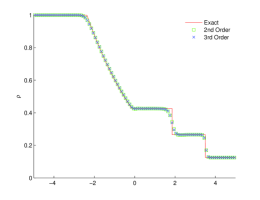
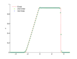
Refer to caption
Refer to caption
Refer to caption
Refer to caption
Figure 8.1: Numerical solutions of Sod problem: 100 grid point are used.

8.2 123 problem

This example was first proposed by [9]. The initial data is given with (ρ,u,p)=(1,2,0.4)𝜌𝑢𝑝120.4(\rho,u,p)=(1,2,0.4) for 5x<05𝑥0-5\leq x<0 and (ρ,u,p)=(1,2,0.4)𝜌𝑢𝑝120.4(\rho,u,p)=(1,2,0.4) for 0x<50𝑥50\leq x<5. The numerical solutions at time t=1.2𝑡1.2t=1.2 are shown in Fig. 8.2. This test case demonstrates the ability of the GRP schemes to preserve the positivity of the density, pressure and internal energy. Again, the internal energy profile conforms the better performance of third-order scheme.
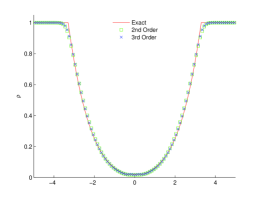
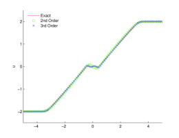
Refer to caption
Refer to caption
Refer to caption
Refer to caption
Figure 8.2: Numerical solutions of 123 problem. 100 grid point are used.

8.3 Woodward-Colella blast wave problem

This is a problem proposed by [26]. The diatomic gas is initially at rest, and the density is unit everywhere. The pressure is p=1000𝑝1000p=1000 for 0x<100𝑥100\leq x<10 and p=100𝑝100p=100 for 90x<10090𝑥10090\leq x<100, while it is only p=0.01𝑝0.01p=0.01 in 10x<9010𝑥9010\leq x<90. Reflecting boundary conditions are applied at both ends and the output time is t=3.8𝑡3.8t=3.8. Numerical solutions with 400 points are shown in Fig. 8.3 to exhibit the performance of both schemes. This test case clearly demonstrates the capability of both schemes in the capturing of strong shock waves. The third-order scheme capture much sharper solution than the second-order scheme in the density and internal energy distribution.
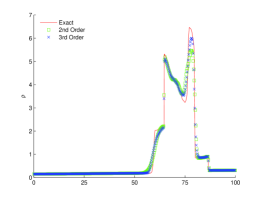
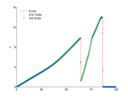
Refer to caption
Refer to caption
Refer to caption
Refer to caption
Figure 8.3: Numerical solutions of Woodward-Colella blast problem. 400 grid point are used.

8.4 Shock-density wave interaction

The Mach 333 shock-entropy wave interaction [20] is specified by the initial condition: (ρ,u,p)=(3.57134,2.629369,10.33333)𝜌𝑢𝑝3.571342.62936910.33333(\rho,u,p)=(3.57134,2.629369,10.33333) for 0x<10𝑥10\leq x<1 and (ρ,u,p)=(1+0.2sin(kx),0,1)𝜌𝑢𝑝10.2𝑘𝑥01(\rho,u,p)=(1+0.2\sin(kx),0,1) for 1x101𝑥101\leq x\leq 10 with k=5𝑘5k=5. The solution of this problem consists of a number of shocklets and fine scales structures which are located behind a right-going main shock. The computed density profile with 400 points, at t=2.0𝑡2.0t=2.0, is shown in Fig. 8.4. Again the third-order scheme works better and captures much finer scale structures at high frequency waves behind the shock.
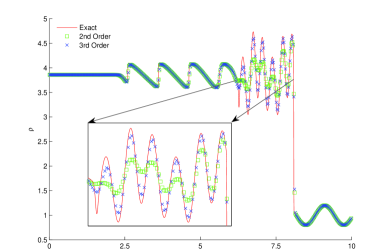
Refer to caption
Figure 8.4: Numerical solutions of shock-density wave problem. 400 grid point are used.

8.5 Steady flow in a converging-diverging nozzle

We now use the examples in [4, Sect. 6.5] to test the ability of the GRP schemes to attain the steady state of a flow. Consider a flow in a converging-diverging nozzle, which occupies the internal 0x10𝑥10\leq x\leq 1 and has a smooth cross-sectional area function A(x)𝐴𝑥A(x) given by the following expression:

A(x)={Ainexp(log(Ain)sin2(2πx)),0x<0.25;Aexexp(log(Aex)sin2(2π(1x)3)),0.25x1,𝐴𝑥casessubscript𝐴insubscript𝐴insuperscript22𝜋𝑥0𝑥0.25subscript𝐴exsubscript𝐴exsuperscript22𝜋1𝑥30.25𝑥1A(x)=\begin{cases}A_{\textrm{in}}\exp\big{(}-\log(A_{\textrm{in}})\sin^{2}(2\pi x)\big{)},&0\leq x<0.25;\\ A_{\textrm{ex}}\exp\left(-\log(A_{\textrm{ex}})\sin^{2}\left(\frac{2\pi(1-x)}{3}\right)\right),&0.25\leq x\leq 1,\end{cases} (8.25)

where Ain=4.8643subscript𝐴in4.8643A_{\textrm{in}}=4.8643 and Aex=4.2346subscript𝐴ex4.2346A_{\textrm{ex}}=4.2346. See Fig. 8.5. For a steady duct flow of a perfect gas, the Mach number M(x)=u(x)/c(x)𝑀𝑥𝑢𝑥𝑐𝑥M(x)=u(x)/c(x) is determined by A(x)𝐴𝑥A(x) through the algebraic relation

[A(x)]2=1[M(x)]2[2γ+1(1+γ12[M(x)]2)]γ+1γ1.superscriptdelimited-[]𝐴𝑥21superscriptdelimited-[]𝑀𝑥2superscriptdelimited-[]2𝛾11𝛾12superscriptdelimited-[]𝑀𝑥2𝛾1𝛾1[A(x)]^{2}=\frac{1}{[M(x)]^{2}}\left[\frac{2}{\gamma+1}\left(1+\frac{\gamma-1}{2}[M(x)]^{2}\right)\right]^{\frac{\gamma+1}{\gamma-1}}. (8.26)

Then the steady flow profiles in the nozzle are given by

p(x)=p0(1+γ12[M(x)]2)γγ1,ρ(x)=ρ0(1+γ12[M(x)]2)1γ1,u(x)=M(x)(γp(x)/ρ(x)),\begin{split}&p(x)=p_{0}\left(1+\frac{\gamma-1}{2}[M(x)]^{2}\right)^{-\frac{\gamma}{\gamma-1}},\\ &\rho(x)=\rho_{0}\left(1+\frac{\gamma-1}{2}[M(x)]^{2}\right)^{-\frac{1}{\gamma-1}},\\ &u(x)=M(x)\sqrt{(}\gamma p(x)/\rho(x)),\end{split} (8.27)

for the flow being smooth, where ρ0subscript𝜌0\rho_{0} and p0subscript𝑝0p_{0} need to be specified.

The initial data we use are

U(x,0)={UL=(ρ0,0,pb),0<x<0.25,UR=(ρ0(pb/p0)1/γ,0,pb),0.25<x<1,𝑈𝑥0casessubscript𝑈𝐿subscript𝜌00subscript𝑝𝑏0𝑥0.25subscript𝑈𝑅subscript𝜌0superscriptsubscript𝑝𝑏subscript𝑝01𝛾0subscript𝑝𝑏0.25𝑥1U(x,0)=\begin{cases}U_{L}=(\rho_{0},0,p_{b}),&0<x<0.25,\\ U_{R}=(\rho_{0}(p_{b}/p_{0})^{1/\gamma},0,p_{b}),&0.25<x<1,\end{cases} (8.28)

where pbsubscript𝑝𝑏p_{b} is a constant determined by the steady state solution at x=1𝑥1x=1. We consider two cases. In both cases we take ρ0=p0=0subscript𝜌0subscript𝑝00\rho_{0}=p_{0}=0 and A(x)𝐴𝑥A(x) as in (8.25).

  1. (A)

    A smooth flow where p(1)=0.0272237𝑝10.0272237p(1)=0.0272237 is obtained from (8.27) by taking x=1𝑥1x=1 in (8.26), leading to M(1)=3𝑀13M(1)=3.

  2. (B)

    Setting p(1)=0.4𝑝10.4p(1)=0.4 leads to a discontinuous steady state solution, as shown by solid lines in Fig. 8.8.

We use the strategy in [4, Sect. 6.5] to deal with the boundary conditions at x=0𝑥0x=0 and 111. In both cases, the number of grid points used are 22. As shown in Fig. 8.6 and 8.8, both of the GRP solutions at t=15.5𝑡15.5t=15.5 are good agreement with the exact solution. The third-order GRP solutions are closer to the analytical solutions than the second-order ones. Moreover, as shown in Fig. 8.7, the GRP solutions almost attain the steady state at time t=2.5𝑡2.5t=2.5. This shows that the GRP solutions converges to steady solution quickly.

Refer to caption
Figure 8.5: Nozzle contour.
Refer to caption
Refer to caption
Figure 8.6: Large time flow in Laval nozzle: Case A. 22 grid points are used, at time t=15.5𝑡15.5t=15.5.
Refer to caption
Refer to caption
Figure 8.7: Large time flow in Laval nozzle: Case B. 22 grid points are used, at time t=2.5𝑡2.5t=2.5.
Refer to caption
Refer to caption
Figure 8.8: Large time flow in Laval nozzle: Case B. 22 grid points are used, at time t=15.5𝑡15.5t=15.5.

Appendix A Formulae in Section 7.1

For the general case of γ>1𝛾1\gamma>1, the L-equations of w=(S,ψ)subscriptw𝑆𝜓\textbf{{w}}_{-}=(S,\psi) in Section 7.1 yield

DλS(0,β)=A1(ψLβ)γ+1γ1,Dλψ(0,β)=A2(ψLβ)γ+12(γ1)+A3(β)(ψLβ)2γγ1+Z0(β)(ψLβ)γ+12(γ1),formulae-sequencesubscript𝐷subscript𝜆𝑆0𝛽subscript𝐴1superscriptsubscript𝜓𝐿𝛽𝛾1𝛾1subscript𝐷subscript𝜆𝜓0𝛽subscript𝐴2superscriptsubscript𝜓𝐿𝛽𝛾12𝛾1subscript𝐴3𝛽superscriptsubscript𝜓𝐿𝛽2𝛾𝛾1subscript𝑍0𝛽superscriptsubscript𝜓𝐿𝛽𝛾12𝛾1\begin{split}&D_{\lambda_{-}}S(0,\beta)=A_{1}(\psi_{L}-\beta)^{\frac{\gamma+1}{\gamma-1}},\\ &D_{\lambda_{-}}\psi(0,\beta)=A_{2}(\psi_{L}-\beta)^{\frac{\gamma+1}{2(\gamma-1)}}+A_{3}(\beta)(\psi_{L}-\beta)^{\frac{2\gamma}{\gamma-1}}+Z_{0}(\beta)(\psi_{L}-\beta)^{\frac{\gamma+1}{2(\gamma-1)}},\end{split} (A.29)

where A2=A~2Z0(βL)subscript𝐴2subscript~𝐴2subscript𝑍0subscript𝛽𝐿A_{2}=\tilde{A}_{2}-Z_{0}(\beta_{L}) and

Z0(β)={B1(ψLβ)γ32(γ1)+B2(ψLβ)3γ52(γ1),ifγ3,5/3;ψL2A(x)A(x)ln(ψLβ)+B2(ψLβ)3γ52(γ1),ifγ=3;B1ψL(ψLβ)γ32(γ1)38A(x)A(x)ln(ψLβ),ifγ=5/3,subscript𝑍0𝛽casessubscript𝐵1superscriptsubscript𝜓𝐿𝛽𝛾32𝛾1subscript𝐵2superscriptsubscript𝜓𝐿𝛽3𝛾52𝛾1if𝛾353subscript𝜓𝐿2superscript𝐴𝑥𝐴𝑥subscript𝜓𝐿𝛽subscript𝐵2superscriptsubscript𝜓𝐿𝛽3𝛾52𝛾1if𝛾3subscript𝐵1subscript𝜓𝐿superscriptsubscript𝜓𝐿𝛽𝛾32𝛾138superscript𝐴𝑥𝐴𝑥subscript𝜓𝐿𝛽if𝛾53Z_{0}(\beta)=\begin{cases}B_{1}(\psi_{L}-\beta)^{\frac{\gamma-3}{2(\gamma-1)}}+B_{2}(\psi_{L}-\beta)^{\frac{3\gamma-5}{2(\gamma-1)}},&\textrm{if}\ \gamma\neq 3,5/3;\\[5.69054pt] \frac{\psi_{L}}{2}\frac{A^{\prime}(x)}{A(x)}\ln(\psi_{L}-\beta)+B_{2}(\psi_{L}-\beta)^{\frac{3\gamma-5}{2(\gamma-1)}},&\textrm{if}\ \gamma=3;\\[5.69054pt] B_{1}\psi_{L}(\psi_{L}-\beta)^{\frac{\gamma-3}{2(\gamma-1)}}-\frac{3}{8}\frac{A^{\prime}(x)}{A(x)}\ln(\psi_{L}-\beta),&\textrm{if}\ \gamma=5/3,\end{cases}
A1=(ψLβL)γ+1γ1DλS(0,βL),subscript𝐴1superscriptsubscript𝜓𝐿subscript𝛽𝐿𝛾1𝛾1subscript𝐷subscript𝜆𝑆0subscript𝛽𝐿\displaystyle A_{1}=(\psi_{L}-\beta_{L})^{-\frac{\gamma+1}{\gamma-1}}D_{\lambda_{-}}S(0,\beta_{L}),
A~2=1γ(3γ1)SL(ψLβL)γ32(γ1)DλS(βL)+(ψLβL)γ+12(γ1)Dλψ(βL).subscript~𝐴21𝛾3𝛾1subscript𝑆𝐿superscriptsubscript𝜓𝐿subscript𝛽𝐿𝛾32𝛾1subscript𝐷subscript𝜆𝑆subscript𝛽𝐿superscriptsubscript𝜓𝐿subscript𝛽𝐿𝛾12𝛾1subscript𝐷subscript𝜆𝜓subscript𝛽𝐿\displaystyle\tilde{A}_{2}=-\frac{1}{\gamma(3\gamma-1)S_{L}}(\psi_{L}-\beta_{L})^{\frac{\gamma-3}{2(\gamma-1)}}D_{\lambda_{-}}S(\beta_{L})+(\psi_{L}-\beta_{L})^{-\frac{\gamma+1}{2(\gamma-1)}}D_{\lambda_{-}}\psi(\beta_{L}).

The coefficients Aisubscript𝐴𝑖A_{i}, Bjsubscript𝐵𝑗B_{j}, Cksubscript𝐶𝑘C_{k} are defined as in Table A.1 and A.2.

Table A.1: The coefficients A3,,A19subscript𝐴3subscript𝐴19A_{3},\cdots,A_{19} and B1,,B12subscript𝐵1subscript𝐵12B_{1},\cdots,B_{12}
A3subscript𝐴3A_{3} 1γ(3γ1)SLA11𝛾3𝛾1subscript𝑆𝐿subscript𝐴1\frac{1}{\gamma(3\gamma-1)S_{L}}A_{1} B1subscript𝐵1B_{1} (γ1γ3)ψLA(x)A(x)𝛾1𝛾3subscript𝜓𝐿superscript𝐴𝑥𝐴𝑥\left(\frac{\gamma-1}{\gamma-3}\right)\psi_{L}\frac{A^{\prime}(x)}{A(x)}
A4subscript𝐴4A_{4} 1γ(γ+1)SLA11𝛾𝛾1subscript𝑆𝐿subscript𝐴1-\frac{1}{\gamma(\gamma+1)S_{L}}A_{1} B2subscript𝐵2B_{2} 2(γ1)(γ+1)(3γ5)A(x)A(x)2𝛾1𝛾13𝛾5superscript𝐴𝑥𝐴𝑥-\frac{2(\gamma-1)}{(\gamma+1)(3\gamma-5)}\frac{A^{\prime}(x)}{A(x)}
A5subscript𝐴5A_{5} γ14A2𝛾14subscript𝐴2\frac{\gamma-1}{4}A_{2} B3subscript𝐵3B_{3} γ1γ+1A(x)A(x)𝛾1𝛾1superscript𝐴𝑥𝐴𝑥\frac{\gamma-1}{\gamma+1}\frac{A^{\prime}(x)}{A(x)}
A6subscript𝐴6A_{6} γ14(A3A4)𝛾14subscript𝐴3subscript𝐴4\frac{\gamma-1}{4}(A_{3}-A_{4}) B4subscript𝐵4B_{4} 2(γ1)(γ+1)2A(x)A(x)2𝛾1superscript𝛾12superscript𝐴𝑥𝐴𝑥-\frac{2(\gamma-1)}{(\gamma+1)^{2}}\frac{A^{\prime}(x)}{A(x)}
A7subscript𝐴7A_{7} (3γ)(γ+1)8(γ1)A23𝛾𝛾18𝛾1subscript𝐴2-\frac{(3-\gamma)(\gamma+1)}{8(\gamma-1)}A_{2} B5subscript𝐵5B_{5} γ14(B1B3)𝛾14subscript𝐵1subscript𝐵3\frac{\gamma-1}{4}(B_{1}-B_{3})
A8subscript𝐴8A_{8} 2γγ1(3γ4A3+1+γ4A4)2𝛾𝛾13𝛾4subscript𝐴31𝛾4subscript𝐴4-\frac{2\gamma}{\gamma-1}\left(\frac{3-\gamma}{4}A_{3}+\frac{1+\gamma}{4}A_{4}\right) B6subscript𝐵6B_{6} γ14(B2B4)𝛾14subscript𝐵2subscript𝐵4\frac{\gamma-1}{4}(B_{2}-B_{4})
A9subscript𝐴9A_{9} 1γ(γ1)SL2A11𝛾𝛾1superscriptsubscript𝑆𝐿2subscript𝐴1\frac{1}{\gamma(\gamma-1)S_{L}^{2}}A_{1} B7subscript𝐵7B_{7} 3γ4B1γ+14B33𝛾4subscript𝐵1𝛾14subscript𝐵3-\frac{3-\gamma}{4}B_{1}-\frac{\gamma+1}{4}B_{3}
A10subscript𝐴10A_{10} 12γ(γ1)SLA712𝛾𝛾1subscript𝑆𝐿subscript𝐴7-\frac{1}{2\gamma(\gamma-1)S_{L}}A_{7} B8subscript𝐵8B_{8} 3γ2B2γ+12B43𝛾2subscript𝐵2𝛾12subscript𝐵4-\frac{3-\gamma}{2}B_{2}-\frac{\gamma+1}{2}B_{4}
A11subscript𝐴11A_{11} 12γ(γ1)SLA812𝛾𝛾1subscript𝑆𝐿subscript𝐴8-\frac{1}{2\gamma(\gamma-1)S_{L}}A_{8} B9subscript𝐵9B_{9} 12(γ+1γ1)2B5γ+12(γ1)B712superscript𝛾1𝛾12subscript𝐵5𝛾12𝛾1subscript𝐵7\frac{1}{2}\left(\frac{\gamma+1}{\gamma-1}\right)^{2}B_{5}-\frac{\gamma+1}{2(\gamma-1)}B_{7}
A12subscript𝐴12A_{12} (γ+1γ1)2A5γ+12(γ1)A7superscript𝛾1𝛾12subscript𝐴5𝛾12𝛾1subscript𝐴7\left(\frac{\gamma+1}{\gamma-1}\right)^{2}A_{5}-\frac{\gamma+1}{2(\gamma-1)}A_{7} B10subscript𝐵10B_{10} 12(γ+1γ1)2B6γ+12(γ1)B812superscript𝛾1𝛾12subscript𝐵6𝛾12𝛾1subscript𝐵8\frac{1}{2}\left(\frac{\gamma+1}{\gamma-1}\right)^{2}B_{6}-\frac{\gamma+1}{2(\gamma-1)}B_{8}
A13subscript𝐴13A_{13} (γ+1γ1)2A6γ+12(γ1)A8superscript𝛾1𝛾12subscript𝐴6𝛾12𝛾1subscript𝐴8\left(\frac{\gamma+1}{\gamma-1}\right)^{2}A_{6}-\frac{\gamma+1}{2(\gamma-1)}A_{8} B11subscript𝐵11B_{11} 12γ(γ1)SLB712𝛾𝛾1subscript𝑆𝐿subscript𝐵7-\frac{1}{2\gamma(\gamma-1)S_{L}}B_{7}
A14subscript𝐴14A_{14} A9+A11subscript𝐴9subscript𝐴11A_{9}+A_{11} B12subscript𝐵12B_{12} 12γ(γ1)SLB812𝛾𝛾1subscript𝑆𝐿subscript𝐵8-\frac{1}{2\gamma(\gamma-1)S_{L}}B_{8}
A15subscript𝐴15A_{15} 2A1A122subscript𝐴1subscript𝐴122A_{1}A_{12}
A16subscript𝐴16A_{16} 2A1A132subscript𝐴1subscript𝐴132A_{1}A_{13}
A17subscript𝐴17A_{17} A1A10+A2A13+A3A12subscript𝐴1subscript𝐴10subscript𝐴2subscript𝐴13subscript𝐴3subscript𝐴12A_{1}A_{10}+A_{2}A_{13}+A_{3}A_{12}
A18subscript𝐴18A_{18} A1A14+A3A13subscript𝐴1subscript𝐴14subscript𝐴3subscript𝐴13A_{1}A_{14}+A_{3}A_{13}
A19subscript𝐴19A_{19} A2A12subscript𝐴2subscript𝐴12A_{2}A_{12}
Table A.2: The coefficients C1,,C9subscript𝐶1subscript𝐶9C_{1},\cdots,C_{9}
C1subscript𝐶1C_{1} 2A1B92subscript𝐴1subscript𝐵92A_{1}B_{9}
C2subscript𝐶2C_{2} 2A1B102subscript𝐴1subscript𝐵102A_{1}B_{10}
C3subscript𝐶3C_{3} A2B9+A12B1ψL2A7A(x)A(x)subscript𝐴2subscript𝐵9subscript𝐴12subscript𝐵1subscript𝜓𝐿2subscript𝐴7superscript𝐴𝑥𝐴𝑥A_{2}B_{9}+A_{12}B_{1}-\frac{\psi_{L}}{2}A_{7}\frac{A^{\prime}(x)}{A(x)}
C4subscript𝐶4C_{4} A3B9+A1B11+A13B1ψL2A8A(x)A(x)subscript𝐴3subscript𝐵9subscript𝐴1subscript𝐵11subscript𝐴13subscript𝐵1subscript𝜓𝐿2subscript𝐴8superscript𝐴𝑥𝐴𝑥A_{3}B_{9}+A_{1}B_{11}+A_{13}B_{1}-\frac{\psi_{L}}{2}A_{8}\frac{A^{\prime}(x)}{A(x)}
C5subscript𝐶5C_{5} A2B10+A12B2+(A7γ+1A22)A(x)A(x)subscript𝐴2subscript𝐵10subscript𝐴12subscript𝐵2subscript𝐴7𝛾1subscript𝐴22superscript𝐴𝑥𝐴𝑥A_{2}B_{10}+A_{12}B_{2}+\left(\frac{A_{7}}{\gamma+1}-\frac{A_{2}}{2}\right)\frac{A^{\prime}(x)}{A(x)}
C6subscript𝐶6C_{6} A3B10+A1B12+A13B2+(A8γ+1A3+A42)A(x)A(x)subscript𝐴3subscript𝐵10subscript𝐴1subscript𝐵12subscript𝐴13subscript𝐵2subscript𝐴8𝛾1subscript𝐴3subscript𝐴42superscript𝐴𝑥𝐴𝑥A_{3}B_{10}+A_{1}B_{12}+A_{13}B_{2}+\left(\frac{A_{8}}{\gamma+1}-\frac{A_{3}+A_{4}}{2}\right)\frac{A^{\prime}(x)}{A(x)}
C7subscript𝐶7C_{7} B1B9ψL2B7A(x)A(x)ψL2(A(x)A(x))subscript𝐵1subscript𝐵9subscript𝜓𝐿2subscript𝐵7superscript𝐴𝑥𝐴𝑥superscriptsubscript𝜓𝐿2superscriptsuperscript𝐴𝑥𝐴𝑥B_{1}B_{9}-\frac{\psi_{L}}{2}B_{7}\frac{A^{\prime}(x)}{A(x)}-\psi_{L}^{2}\left(\frac{A^{\prime}(x)}{A(x)}\right)^{{}^{\prime}}
C8subscript𝐶8C_{8} B2B9+B1B10+(ψL2B8+B7γ+1B1+B32)A(x)A(x)+γ+3γ+1ψL(A(x)A(x))subscript𝐵2subscript𝐵9subscript𝐵1subscript𝐵10subscript𝜓𝐿2subscript𝐵8subscript𝐵7𝛾1subscript𝐵1subscript𝐵32superscript𝐴𝑥𝐴𝑥𝛾3𝛾1subscript𝜓𝐿superscriptsuperscript𝐴𝑥𝐴𝑥B_{2}B_{9}+B_{1}B_{10}+\left(-\frac{\psi_{L}}{2}B_{8}+\frac{B_{7}}{\gamma+1}-\frac{B_{1}+B_{3}}{2}\right)\frac{A^{\prime}(x)}{A(x)}+\frac{\gamma+3}{\gamma+1}\psi_{L}\left(\frac{A^{\prime}(x)}{A(x)}\right)^{{}^{\prime}}
C9subscript𝐶9C_{9} B2B10+(B8γ+1B2+B42)A(x)A(x)2γ+1(A(x)A(x))subscript𝐵2subscript𝐵10subscript𝐵8𝛾1subscript𝐵2subscript𝐵42superscript𝐴𝑥𝐴𝑥2𝛾1superscriptsuperscript𝐴𝑥𝐴𝑥B_{2}B_{10}+\left(-\frac{B_{8}}{\gamma+1}-\frac{B_{2}+B_{4}}{2}\right)\frac{A^{\prime}(x)}{A(x)}-\frac{2}{\gamma+1}\left(\frac{A^{\prime}(x)}{A(x)}\right)^{{}^{\prime}}

The function Z1(β)subscript𝑍1𝛽Z_{1}(\beta) and Z2(β)subscript𝑍2𝛽Z_{2}(\beta) in Proposition 7.1 are as follows

Z1(β)=2(γ1)3γ1A15(ψLβ)3γ+12(γ1)A16ln(ψLβ)subscript𝑍1𝛽2𝛾13𝛾1subscript𝐴15superscriptsubscript𝜓𝐿𝛽3𝛾12𝛾1subscript𝐴16subscript𝜓𝐿𝛽\displaystyle Z_{1}(\beta)=\frac{2(\gamma-1)}{3\gamma-1}A_{15}(\psi_{L}-\beta)^{\frac{-3\gamma+1}{2(\gamma-1)}}-A_{16}\ln(\psi_{L}-\beta)
+γ1γ+1C1(ψLβ)(γ+1γ1)+γ12C2(ψLβ)2γ1,𝛾1𝛾1subscript𝐶1superscriptsubscript𝜓𝐿𝛽𝛾1𝛾1𝛾12subscript𝐶2superscriptsubscript𝜓𝐿𝛽2𝛾1\displaystyle\hskip 56.9055pt+\frac{\gamma-1}{\gamma+1}C_{1}(\psi_{L}-\beta)^{-\left(\frac{\gamma+1}{\gamma-1}\right)}+\frac{\gamma-1}{2}C_{2}(\psi_{L}-\beta)^{\frac{-2}{\gamma-1}},
Z2(β)=12γ2SL(ψLβ)2γ1Dλ2S(β)+γ1γ+1[A15γ2SL2A17](ψLβ)γ+12(γ1)subscript𝑍2𝛽12superscript𝛾2subscript𝑆𝐿superscriptsubscript𝜓𝐿𝛽2𝛾1superscriptsubscript𝐷subscript𝜆2𝑆𝛽𝛾1𝛾1delimited-[]subscript𝐴15superscript𝛾2subscript𝑆𝐿2subscript𝐴17superscriptsubscript𝜓𝐿𝛽𝛾12𝛾1\displaystyle Z_{2}(\beta)=\frac{1}{2\gamma^{2}S_{L}}(\psi_{L}-\beta)^{-\frac{2}{\gamma-1}}D_{\lambda_{-}}^{2}S(\beta)+\frac{\gamma-1}{\gamma+1}\left[\frac{A_{15}}{\gamma^{2}S_{L}}-2A_{17}\right](\psi_{L}-\beta)^{\frac{\gamma+1}{2(\gamma-1)}}
+γ12γ[A162γ2SLA18](ψLβ)2γγ1+A19(ψLβ)1𝛾12𝛾delimited-[]subscript𝐴162superscript𝛾2subscript𝑆𝐿subscript𝐴18superscriptsubscript𝜓𝐿𝛽2𝛾𝛾1subscript𝐴19superscriptsubscript𝜓𝐿𝛽1\displaystyle\hskip 56.9055pt+\frac{\gamma-1}{2\gamma}\left[\frac{A_{16}}{2\gamma^{2}S_{L}}-A_{18}\right](\psi_{L}-\beta)^{\frac{2\gamma}{\gamma-1}}+A_{19}(\psi_{L}-\beta)^{-1}
+[C12γ2SLC4](ψLβ)+[C24γ2SLC62](ψLβ)2delimited-[]subscript𝐶12superscript𝛾2subscript𝑆𝐿subscript𝐶4subscript𝜓𝐿𝛽delimited-[]subscript𝐶24superscript𝛾2subscript𝑆𝐿subscript𝐶62superscriptsubscript𝜓𝐿𝛽2\displaystyle\hskip 56.9055pt+\left[\frac{C_{1}}{2\gamma^{2}S_{L}}-C_{4}\right](\psi_{L}-\beta)+\left[\frac{C_{2}}{4\gamma^{2}S_{L}}-\frac{C_{6}}{2}\right](\psi_{L}-\beta)^{2}
+2(γ1)γ+1C3(ψLβ)γ+12(γ1)2(γ1)γ3C5(ψLβ)γ32(γ1)2𝛾1𝛾1subscript𝐶3superscriptsubscript𝜓𝐿𝛽𝛾12𝛾12𝛾1𝛾3subscript𝐶5superscriptsubscript𝜓𝐿𝛽𝛾32𝛾1\displaystyle\hskip 56.9055pt+\frac{2(\gamma-1)}{\gamma+1}C_{3}(\psi_{L}-\beta)^{-\frac{\gamma+1}{2(\gamma-1)}}-\frac{2(\gamma-1)}{\gamma-3}C_{5}(\psi_{L}-\beta)^{\frac{\gamma-3}{2(\gamma-1)}}
+γ12C7(ψLβ)2γ1γ1γ3C8(ψLβ)γ3γ1𝛾12subscript𝐶7superscriptsubscript𝜓𝐿𝛽2𝛾1𝛾1𝛾3subscript𝐶8superscriptsubscript𝜓𝐿𝛽𝛾3𝛾1\displaystyle\hskip 56.9055pt+\frac{\gamma-1}{2}C_{7}(\psi_{L}-\beta)^{-\frac{2}{\gamma-1}}-\frac{\gamma-1}{\gamma-3}C_{8}(\psi_{L}-\beta)^{\frac{\gamma-3}{\gamma-1}}
γ12(γ2)C9(ψLβ)2(γ2)γ1.𝛾12𝛾2subscript𝐶9superscriptsubscript𝜓𝐿𝛽2𝛾2𝛾1\displaystyle\hskip 56.9055pt-\frac{\gamma-1}{2(\gamma-2)}C_{9}(\psi_{L}-\beta)^{\frac{2(\gamma-2)}{\gamma-1}}.

References

  • [1] M. Ben-Artzi, J. Falcovitz, A second-order Godunov-type scheme for compressible fluid dynamics, J. Comput. Phys. 55 (1) (1984) 1–32.
  • [2] M. Ben-Artzi, J. Falcovitz, An upwind second-order scheme for compressible duct flows, SIAM J. Sci. Stat. Comput. 7 (3) (1986) 744–768.
  • [3] M. Ben-Artzi, The generalized Riemann problem for reactive flows, J. Comput. Phys. 81 (1) (1989) 70–101.
  • [4] M. Ben-Artzi, J. Falcovitz, Generalized Riemann problems in computational fluid dynamics. Cambridge Monographs on Applied and Computational Mathematics, 11, 2003.
  • [5] M. Ben-Artzi, J. Li and G. Warnecke, A direct Eulerian GRP scheme for compressible fluid flows, J. Comput. Phys. 218 (2006) 19–34.
  • [6] M. Ben-Artzi, J. Li, Hyperbolic balance laws: Riemann invariants and the generalized Riemann problem, Numer. Math. 106 (2007) 369–425.
  • [7] A. Bourgeade, P. LeFloch, P. A. Raviart, An asymptotic expansion for the solution of the generalized Riemann problem. II. Application to the equations of gas dynamics, Ann. Inst. H. Poincar Anal. NonLinaire 6 (6) (1989) 437–480.
  • [8] C. E. Castro, E. F. Toro, Solver for the high-order Riemann problem for hyperbolic balance laws, J. Comput. Phys. 227, (2008) 2481–2513.
  • [9] B. Einfeldt, C.D. Munz, P.L. Roe, B. Sjögreen, On Godunov-type methods near low densities, J. Comput. Phys. 92 (1991) 273–295.
  • [10] S. K. Godunov, A finite-difference method for the numerical computation of discontinuous solutions of the equations of fluid dynamics, Mat. Sb. 47 (1959) 271–295.
  • [11] A. Harten, High resolution schemes for hyperbolic conservation laws, J. Comput. Phys. 49, (1983) 357–393.
  • [12] A. Harten, B. Engquist, S. Osher, and S. Chakravarthy, Uniformly high order essentially non-oscillatory schemes III, J. Comput. Phys. 71 (1987) 231–303.
  • [13] S. Jin, A steady-state capturing method for hyperbolic systems with geometrical source terms, Math. Model. Numer. Anal. 35 (4) (2001) 631–645.
  • [14] P. LeFloch, P.-A. Raviart, An asymptotic expansion for the solution of the generalized Riemann problem. I. General theory, Ann. Inst. H. Poincaré Anal. Non Liné aire 5 (2) (1988) 179–207.
  • [15] G. Montecinos, C. E. Castro, M. Dumbser, E. F. Toro, Comparison of solver for the generalized Riemann problem for hyperbolic systems with source terms, J. Comput. Phys. 231 (2012) 6472–6494.
  • [16] J. Li, G. Chen, The generalized Riemann problem method for the shallow water equations with bottom topography, Int. J. Numer. Meth. Eng. 65 (6) (2006) 834–862.
  • [17] J. Li and J. Qian, A genuinely multidimensional GRP solvers for compressible fluid flows, in preparation, 2013.
  • [18] J. Luo, L.J. Xuan, K. Xu, Comparison of fifth-order WENO scheme and WENO-gas-kinetic scheme for inviscid and viscous flow simulation, Commun. Comput. Phys., Vol. 14, No. 3 (2013) 599–620.
  • [19] C.W. Shu, Essentially non-oscillatory and weighted essentially non-oscillatory schemes for hyperbolic conservation laws, Lecture Notes in Mathematics, Springer, 1998.
  • [20] C.W. Shu, S. Osher, Efficient implementation of essentially non-oscillatory shock-capturing schemes, J. Comput. Phys. 77 (1988) 439–471.
  • [21] G.A. Sod, A survey of several finite difference methods for systems of nonlinear hyperbolic conservation laws, J. Comput. Phys. 27 (1978) 1–31.
  • [22] E.F. Toro, Riemann Solvers and Numerical Methods for Fluid Dynamics: A Practical Introduction, Springer, 1997.
  • [23] E.F. Toro, V.A. Tarev, Derivative Riemann Solvers for systems for conservation laws and ADER methods, J. Comput. Phys. 212 (2006) 150–165.
  • [24] B. van Leer, Towards the ultimate conservative difference scheme II. Monotonicity and conservation combined in a second-order scheme, J. Comput. Phys. 14 (1974) 361–370.
  • [25] B. van Leer, Towards the ultimate conservative difference scheme, V. A second order sequel to Godunov’s method, J. Comput. Phys. 32 (1979) 101–136.
  • [26] P. Woodward, P. Colella, The numerical simulation of two-dimensional fluid flow with strong shocks, J. Comput. Phys. 54 (1984) 115–173.
  • [27] Z.C. Yang, P. He, H.Z. Tang, A direct Eulerian GRP scheme for relativistic hydrodynamics: one-dimensional case, J. Comput. Phys. 230 (2011) 7964–7987.
  • [28] Z.C. Yang, H.Z. Tang, A direct Eulerian GRP scheme for relativistic hydrodynamics: Two-dimensional case, J. Comput. Phys. 231 (2012) 2116–2139.