The incompleteness of complete pseudoscalar-meson photoproduction

Tom Vrancx Tom.Vrancx@UGent.be    Jan Ryckebusch Jan.Ryckebusch@UGent.be    Tom Van Cuyck    Pieter Vancraeyveld Department of Physics and Astronomy,
Ghent University, Proeftuinstraat 86, B-9000 Gent, Belgium
Abstract
Background:

A complete set is a minimum set of observables which allows one to determine the underlying reaction amplitudes unambiguously. Pseudoscalar-meson photoproduction from the nucleon is characterized by four such amplitudes and complete sets involve single- and double-polarization observables.

Purpose:

Identify complete sets of observables, and study how measurements with finite error bars impact their potential to determine the reaction amplitudes unambiguously.

Method:

The authors provide arguments to employ the transversity representation in order to determine the amplitudes in pseudoscalar-meson photoproduction. It is studied whether the amplitudes in the transversity basis for the γpK+Λ𝛾𝑝superscript𝐾Λ\gamma p\to K^{+}\Lambda reaction can be estimated without ambiguity. To this end, data from the GRAAL collaboration and simulations from a realistic model are analyzed.

Results:

It is illustrated that the moduli of normalized transversity amplitudes can be determined from precise single-polarization data. Starting from simulations with achievable experimental resolution, it is quite likely to obtain imaginary solutions for the relative phases of the amplitudes. Also the real solutions face a discrete phase ambiguity which makes it impossible to obtain a statistically significant solution for the relative phases at realistic experimental conditions.

Conclusions:

Single polarization observables are effective in determining the moduli of the amplitudes in a transversity basis. Determining the relative phases of the amplitudes from double-polarization observables is far less evident. The availability of a complete set of observables does not allow one to unambiguously determine the reaction amplitudes with statistical significance.

pacs:
11.80.Cr, 13.60.Le, 24.10.-i, 25.20.Lj

I Introduction

Pseudoscalar-meson photoproduction from the nucleon continues to be an invaluable source of information about the operation of quantum chromodynamics (QCD) in the nonperturbative regime CLAS2012a ; CLAS2012b ; LEGS-GRAAL2012 ; MAMI2012 ; ELSA2012 . Various classes of models, like constituent-quark approaches, have been developed to understand the structure and dynamics of hadrons in the low-energy regime of QCD. Experimental determination of the reaction amplitudes represents the most stringent test of those models and may open up a new chapter in the understanding of the energy eigenvalues and decay properties of hadron states.

Quantum mechanics dictates that measurable quantities can be expressed as bilinear combinations of complex amplitudes. Pseudoscalar meson photoproduction involves only two kinematical degrees of freedom, for example the energy of the incident photon and the scattering angle of the pseudoscalar meson. Since the (real) photon, the target, and the recoiling baryon have two spin degrees of freedom, eight possible amplitudes can be constructed. Due to angular momentum conservation, and depending on the adopted representation, half of these amplitudes either vanish identically or can be expressed in terms of the other four amplitudes. This leaves one with a set of four independent amplitudes. These amplitudes are complex functions (of the two kinematical variables) and therefore eight real functions are to be distinguished: four moduli and four phases. As quantum states are determined up to a constant phase factor, only the relative phases of the amplitudes can be extracted. This means that pseudoscalar photoproduction can be quantified in terms of seven real-valued functions of the two kinematical variables. Equivalently, at fixed kinematics seven real values suffice to determine all observables.

A set containing a minimum number of observables from which, at fixed kinematics, the seven real values can be determined unanimously is referred to as a complete set. In a seminal paper dating back to 1975, Barker, Donnachie, and Storrow argued that a complete set requires nine observables of a specific type Barker:1975bp . In 1996, this was contested by Keaton and Workman Keaton1996 and by Wen-Tai Chiang and Tabakin Chiang:1996em . The latter proved that eight well-chosen observables suffice to unambiguously determine the four moduli and three independent relative phases.

In theory, a complete set of eight observables suffices to retrieve the generating seven variables. The need for an additional observable (a set of eight equations involving only seven variables) to uniquely determine the relative phases, is a reflection of the fact that the latter are linked to the observables through nonlinear equations. A set of seven well-chosen observables generally yields multiple solutions for the phases. Therefore, an extra observable is required to mark the correct solution. In reality, however, observables have a finite precision and deviate from the exact values. This compromises the solution of the phase ambiguity Ireland2010 . It then remains a question whether a set of eight observables is still sufficient to reach a situation of complete knowledge about the amplitudes.

Thanks to recent technological advances in producing high-quality polarized beams and in developing polarized nucleon targets Hoblit2009 , it becomes possible to measure a sufficiently large amount of single- and double-polarization observables in pion and kaon photoproduction. As a result, a status of complete quantum mechanical information of pseudoscalar meson photoproduction comes within reach. The self-analyzing character of the ΛΛ\Lambda is an enormous asset for achieving truly complete measurements for γpK+Λ𝛾𝑝superscript𝐾Λ\gamma p\to K^{+}\Lambda and experimental efforts are under way CLAS2012b . For example, the CLAS collaboration at Jefferson Lab has many γpK+Λ𝛾𝑝superscript𝐾Λ\gamma p\to K^{+}\Lambda polarization data in the pipeline.

It should be stressed that in the quality and quantity of the experimental results, there is some kind of hierarchy. Indeed, double-polarization data is most often outnumbered by single-polarization results, which in their turn are outnumbered by the size of the differential cross section database. In view of this, the transversity representation of the amplitudes is a very promising one. Indeed, in this basis the single-polarization observables are linked to the squared moduli of the amplitudes by means of linear equations. Accordingly, the transversity basis occupies a central position in this work.

The outline of the remainder of this paper is as follows. In Sec. II, the transversity amplitudes are introduced and all possible observables for pseudoscalar meson photoproduction are expressed in this basis. In Sec. III, Wen-Tai Chiang and Tabakin’s formalism for solving complete sets is briefly reviewed. This formalism is solid in the exact case. When experimental uncertainty is involved, however, a consistency issue for a unique determination of the phases arises. A method to resolve this inconsistency is proposed. As a test of this method, in Sec. IV it is applied to simulations from a realistic model for the γpK+Λ𝛾𝑝superscript𝐾Λ\gamma p\to K^{+}\Lambda reaction. The conclusions are summarized in Sec. V. In the Appendix, both the helicity and the CGLN expansions of the observables are considered, and a connection to the transversity basis is established.

II Observables for pseudoscalar meson production

II.1 Reaction amplitudes

The convention is adopted that the xz𝑥𝑧xz–plane coincides with the reaction plane and that the positive z𝑧z–axis is along the direction of the photon’s three-momentum. The two independent kinematic variables that will be considered throughout this work are the total energy of the reaction, or invariant mass, W𝑊W and the scattering angle of the pseudoscalar meson in the center-of-mass frame θc.m.subscript𝜃c.m.\theta_{\text{c.m.}}. As mentioned in Sec. I, pseudoscalar-meson photoproduction can be quantified by four complex reaction amplitudes i(W,cosθc.m.)subscript𝑖𝑊subscript𝜃c.m.\mathcal{M}_{i}(W,\cos\theta_{\text{c.m.}}) (i=1,2,3,4)𝑖1234(i=1,2,3,4). The unpolarized differential cross section, for example, is given by

dσ(W,cosθc.m.)dΩ=ϱi=14|i(W,cosθc.m.)|2,d𝜎𝑊subscript𝜃c.m.dΩitalic-ϱsuperscriptsubscript𝑖14superscriptsubscript𝑖𝑊subscript𝜃c.m.2\frac{\mathrm{d}\sigma(W,\cos\theta_{\text{c.m.}})}{\mathrm{d}\Omega}=\varrho\sum_{i=1}^{4}\bigl{|}\mathcal{M}_{i}(W,\cos\theta_{\text{c.m.}})\bigr{|}^{2}, (1)

where ϱitalic-ϱ\varrho is a kinematic factor. There are various equivalent representations for the isubscript𝑖\mathcal{M}_{i}, all of which have a distinct kinematic factor ϱitalic-ϱ\varrho. The representation is determined by the choices made with regard to the quantization axis of the involved particles with a non-vanishing spin: the nucleon target, the incoming photon, and the recoiling baryon.

The Dirac spinors for a particle with rest mass m𝑚m, four-momentum pμ=(E,p)superscript𝑝𝜇𝐸𝑝p^{\mu}=(E,\vec{p}), and a spin vector with polar angles (θ,ϕ)𝜃italic-ϕ(\theta,\phi) are defined as

u±(pμ,θ,ϕ)=12m(E+m)((E+m)I2σp)s±(θ,ϕ),subscript𝑢plus-or-minussuperscript𝑝𝜇𝜃italic-ϕ12𝑚𝐸𝑚matrix𝐸𝑚subscript𝐼2𝜎𝑝subscript𝑠plus-or-minus𝜃italic-ϕ\displaystyle u_{\pm}(p^{\mu},\theta,\phi)=\frac{1}{\sqrt{2m(E+m)}}\begin{pmatrix}(E+m)I_{2}\\ \vec{\sigma}\cdot\vec{p}\end{pmatrix}s_{\pm}(\theta,\phi), (2)

following the Bjørken-Drell convention BjorkenDrellBook . Here, I2subscript𝐼2I_{2} represents the 2×2222\times 2 identity matrix and σ=(σx,σy,σz)𝜎subscript𝜎𝑥subscript𝜎𝑦subscript𝜎𝑧\vec{\sigma}=(\sigma_{x},\sigma_{y},\sigma_{z}) is the Pauli vector. Further, the Pauli spinors s+(θ,ϕ)subscript𝑠𝜃italic-ϕs_{+}(\theta,\phi) (“spin up”) and s(θ,ϕ)subscript𝑠𝜃italic-ϕs_{-}(\theta,\phi) (“spin down”) are given by

s+(θ,ϕ)subscript𝑠𝜃italic-ϕ\displaystyle s_{+}(\theta,\phi) =(cosθ2eiϕsinθ2),absentmatrix𝜃2superscript𝑒𝑖italic-ϕ𝜃2\displaystyle=\begin{pmatrix}\cos\frac{\theta}{2}\\ e^{i\phi}\sin\frac{\theta}{2}\end{pmatrix},
s(θ,ϕ)subscript𝑠𝜃italic-ϕ\displaystyle s_{-}(\theta,\phi) =(eiϕsinθ2cosθ2).absentmatrixsuperscript𝑒𝑖italic-ϕ𝜃2𝜃2\displaystyle=\begin{pmatrix}-e^{-i\phi}\sin\frac{\theta}{2}\\ \cos\frac{\theta}{2}\end{pmatrix}. (3)

The following shorthand notations are introduced

|±xsubscriptketplus-or-minus𝑥\displaystyle|\pm\rangle_{x} =u±(pμ,π2,0),absentsubscript𝑢plus-or-minussuperscript𝑝𝜇𝜋20\displaystyle=u_{\pm}(p^{\mu},\tfrac{\pi}{2},0),
|±ysubscriptketplus-or-minus𝑦\displaystyle|\pm\rangle_{y} =u±(pμ,π2,π2),absentsubscript𝑢plus-or-minussuperscript𝑝𝜇𝜋2𝜋2\displaystyle=u_{\pm}(p^{\mu},\tfrac{\pi}{2},\tfrac{\pi}{2}),
|±zsubscriptketplus-or-minus𝑧\displaystyle|\pm\rangle_{z} =u±(pμ,0,0).absentsubscript𝑢plus-or-minussuperscript𝑝𝜇00\displaystyle=u_{\pm}(p^{\mu},0,0). (4)

Using Eq. (2) it can readily be verified that the |±xsubscriptketplus-or-minus𝑥|\pm\rangle_{x} and |±zsubscriptketplus-or-minus𝑧|\pm\rangle_{z} can be expressed in terms of the |±ysubscriptketplus-or-minus𝑦|\pm\rangle_{y} as follows

|±xsubscriptketplus-or-minus𝑥\displaystyle|\pm\rangle_{x} =1i2(|y±|+y),absentminus-or-plus1𝑖2plus-or-minussubscriptket𝑦subscriptket𝑦\displaystyle=\frac{1\mp i}{2}\Bigl{(}|-\rangle_{y}\pm|+\rangle_{y}\Bigr{)},
|±zsubscriptketplus-or-minus𝑧\displaystyle|\pm\rangle_{z} =12(|±yi|y).absent12subscriptketplus-or-minus𝑦𝑖subscriptketminus-or-plus𝑦\displaystyle=\frac{1}{\sqrt{2}}\Bigl{(}|\pm\rangle_{y}-i|\mp\rangle_{y}\Bigr{)}. (5)

The i(W,cosθc.m.)subscript𝑖𝑊subscript𝜃c.m.\mathcal{M}_{i}(W,\cos\theta_{\text{c.m.}}) are the amplitudes of the operator ϵλμJμsubscriptsuperscriptitalic-ϵ𝜇𝜆subscript𝐽𝜇\epsilon^{\mu}_{\lambda}J_{\mu} for a fixed polarization of the initial and final state particles. The ϵλμsubscriptsuperscriptitalic-ϵ𝜇𝜆\epsilon^{\mu}_{\lambda} is the photon’s polarization four-vector and Jμsuperscript𝐽𝜇J^{\mu} the transition current operator. The photon beam polarizations denoted by “=x𝑥\mathcal{B}=x” (+exsubscript𝑒𝑥+\vec{e}_{x} direction) and “=y𝑦\mathcal{B}=y” (+eysubscript𝑒𝑦+\vec{e}_{y} direction) correspond with

ϵxμsubscriptsuperscriptitalic-ϵ𝜇𝑥\displaystyle\epsilon^{\mu}_{x} =(0,1,0,0),absent0100\displaystyle=(0,1,0,0),
ϵyμsubscriptsuperscriptitalic-ϵ𝜇𝑦\displaystyle\epsilon^{\mu}_{y} =(0,0,1,0),absent0010\displaystyle=(0,0,1,0), (6)

and give rise to the following currents

Jxsubscript𝐽𝑥\displaystyle J_{x} =ϵxμJμ,absentsubscriptsuperscriptitalic-ϵ𝜇𝑥subscript𝐽𝜇\displaystyle=\epsilon^{\mu}_{x}J_{\mu},
Jysubscript𝐽𝑦\displaystyle J_{y} =ϵyμJμ.absentsubscriptsuperscriptitalic-ϵ𝜇𝑦subscript𝐽𝜇\displaystyle=\epsilon^{\mu}_{y}J_{\mu}. (7)

The photon beam polarizations denoted by “=±π/4plus-or-minus𝜋4\mathcal{B}=\pm\pi/4” (oblique polarization, ϵ±π/4μ=12(0,1,±1,0)subscriptsuperscriptitalic-ϵ𝜇plus-or-minus𝜋41201plus-or-minus10\epsilon^{\mu}_{\pm\pi/4}=\tfrac{1}{\sqrt{2}}(0,1,\pm 1,0)) and “=±plus-or-minus\mathcal{B}=\pm” (circular polarization, ϵ±μ=12(0,1,±i,0)subscriptsuperscriptitalic-ϵ𝜇plus-or-minus1201plus-or-minus𝑖0\epsilon^{\mu}_{\pm}=\tfrac{1}{\sqrt{2}}(0,1,\pm i,0)) correspond with

J±π/4subscript𝐽plus-or-minus𝜋4\displaystyle J_{\pm\pi/4} =12(Jx±Jy),absent12plus-or-minussubscript𝐽𝑥subscript𝐽𝑦\displaystyle=-\frac{1}{\sqrt{2}}\left(J_{x}\pm J_{y}\right), (8)
J±subscript𝐽plus-or-minus\displaystyle\qquad J_{\pm} =12(Jx±iJy).absent12plus-or-minussubscript𝐽𝑥𝑖subscript𝐽𝑦\displaystyle=-\frac{1}{\sqrt{2}}\left(J_{x}\pm iJ_{y}\right). (9)

II.2 Observables in the transversity basis

The so-called transversity amplitudes bisubscript𝑏𝑖b_{i} express the isubscript𝑖\mathcal{M}_{i} in terms of the spinors |±ysubscriptketplus-or-minus𝑦|\pm\rangle_{y} (quantization axis perpendicular to the reaction plane) and the linear photon polarizations Jxsubscript𝐽𝑥J_{x} and Jysubscript𝐽𝑦J_{y}, i.e.

b1subscript𝑏1\displaystyle b_{1} =+|Jy|+yy,\displaystyle={}_{y}\langle+|J_{y}|+\rangle_{y},
b2subscript𝑏2\displaystyle b_{2} =|Jy|yy,\displaystyle={}_{y}\langle-|J_{y}|-\rangle_{y},
b3subscript𝑏3\displaystyle b_{3} =+|Jx|yy,\displaystyle={}_{y}\langle+|J_{x}|-\rangle_{y},
b4subscript𝑏4\displaystyle b_{4} =|Jx|+yy.\displaystyle={}_{y}\langle-|J_{x}|+\rangle_{y}. (10)

In these definitions, the bra (ket) refers to the recoil (target). The differential cross section for a given beam \mathcal{B}, target 𝒯𝒯\mathcal{T}, and recoil polarization \mathcal{R} is denoted as

ς(,𝒯,)=dσdΩ(,𝒯,).superscript𝜍𝒯superscriptd𝜎dΩ𝒯\displaystyle\varsigma^{(\mathcal{B},\mathcal{T},\mathcal{R})}=\frac{\mathrm{d}\sigma}{\mathrm{d}\Omega}^{(\mathcal{B},\mathcal{T},\mathcal{R})}. (11)

An unpolarized state is denoted by “00”. For example, 𝒯=0𝒯0\mathcal{T}=0 denotes an unpolarized target and in computing the cross section (11) for 𝒯=0𝒯0\mathcal{T}=0, an averaging over both target polarizations is implicitly assumed.

An asymmetry A𝐴A can generally be expressed as

A=ς(1,𝒯1,1)ς(2,𝒯2,2)ς(1,𝒯1,1)+ς(2,𝒯2,2).𝐴superscript𝜍subscript1subscript𝒯1subscript1superscript𝜍subscript2subscript𝒯2subscript2superscript𝜍subscript1subscript𝒯1subscript1superscript𝜍subscript2subscript𝒯2subscript2\displaystyle A=\frac{\varsigma^{(\mathcal{B}_{1},\mathcal{T}_{1},\mathcal{R}_{1})}-\varsigma^{(\mathcal{B}_{2},\mathcal{T}_{2},\mathcal{R}_{2})}}{\varsigma^{(\mathcal{B}_{1},\mathcal{T}_{1},\mathcal{R}_{1})}+\varsigma^{(\mathcal{B}_{2},\mathcal{T}_{2},\mathcal{R}_{2})}}. (12)

A single asymmetry comprises one polarized and two unpolarized states. Hence, there are three possible single-polarization observables, namely the beam asymmetry ΣΣ\Sigma (00\mathcal{B}\neq 0), the target asymmetry T𝑇T (𝒯0𝒯0\mathcal{T}\neq 0), and the recoil asymmetry P𝑃P (00\mathcal{R}\neq 0). The explicit definitions of these three single asymmetries can be found in Table 1. A double asymmetry, involves two polarized and one unpolarized state. There are three types of double asymmetries: the target-recoil asymmetries (1=2=0subscript1subscript20\mathcal{B}_{1}=\mathcal{B}_{2}=0), the beam-recoil asymmetries (𝒯1=𝒯2=0subscript𝒯1subscript𝒯20\mathcal{T}_{1}=\mathcal{T}_{2}=0), and the beam-target asymmetries (1=2=0subscript1subscript20\mathcal{R}_{1}=\mathcal{R}_{2}=0). The definitions for the various double asymmetries are contained in Table 1.

The aim of the current section is to represent the single and double asymmetries in the transversity basis. As representative examples, the transversity expansions of the single asymmetry ΣΣ\Sigma and of the double asymmetry Cxsubscript𝐶𝑥C_{x} are derived. The beam asymmetry ΣΣ\Sigma is defined as

Σ=ς(y,0,0)ς(x,0,0)ς(y,0,0)+ς(x,0,0).Σsuperscript𝜍𝑦00superscript𝜍𝑥00superscript𝜍𝑦00superscript𝜍𝑥00\displaystyle\Sigma=\frac{\varsigma^{(y,0,0)}-\varsigma^{(x,0,0)}}{\varsigma^{(y,0,0)}+\varsigma^{(x,0,0)}}. (13)

Using

ς(y,0,0)superscript𝜍𝑦00\displaystyle\varsigma^{(y,0,0)} =12(ς(y,+y,+y)+ς(y,+y,y)\displaystyle=\frac{1}{2}\Bigl{(}\varsigma^{(y,+y,+y)}+\varsigma^{(y,+y,-y)}
+ς(y,y,+y)+ς(y,y,y)),\displaystyle\quad\,+\varsigma^{(y,-y,+y)}+\varsigma^{(y,-y,-y)}\Bigr{)},
=ϱ2(|+|Jy|+yy=b1|2+||Jy|+yy= 0|2\displaystyle=\frac{\varrho}{2}\Bigl{(}\bigl{|}\underbrace{{}_{y}\langle+|J_{y}|+\rangle_{y}}_{=\,b_{1}}\bigr{|}^{2}+\bigl{|}\underbrace{{}_{y}\langle-|J_{y}|+\rangle_{y}}_{=\,0}\bigr{|}^{2}
+|+|Jy|yy= 0|2+||Jy|yy=b2|2),\displaystyle\quad\,+\bigl{|}\underbrace{{}_{y}\langle+|J_{y}|-\rangle_{y}}_{=\,0}\bigr{|}^{2}+\bigl{|}\underbrace{{}_{y}\langle-|J_{y}|-\rangle_{y}}_{=\,b_{2}}\bigr{|}^{2}\Bigr{)},
=ϱ2(|b1|2+|b2|2),absentitalic-ϱ2superscriptsubscript𝑏12superscriptsubscript𝑏22\displaystyle=\frac{\varrho}{2}\left(|b_{1}|^{2}+|b_{2}|^{2}\right), (14)
and
ς(x,0,0)superscript𝜍𝑥00\displaystyle\varsigma^{(x,0,0)} =12(ς(x,+y,+y)+ς(x,+y,y)\displaystyle=\frac{1}{2}\Bigl{(}\varsigma^{(x,+y,+y)}+\varsigma^{(x,+y,-y)}
+ς(x,y,+y)+ς(x,y,y)),\displaystyle\quad\,+\varsigma^{(x,-y,+y)}+\varsigma^{(x,-y,-y)}\Bigr{)},
=ϱ2(|+|Jx|+yy= 0|2+||Jx|+yy=b4|2\displaystyle=\frac{\varrho}{2}\Bigl{(}\bigl{|}\underbrace{{}_{y}\langle+|J_{x}|+\rangle_{y}}_{=\,0}\bigr{|}^{2}+\bigl{|}\underbrace{{}_{y}\langle-|J_{x}|+\rangle_{y}}_{=\,b_{4}}\bigr{|}^{2}
+|+|Jx|yy=b3|2+||Jx|yy= 0|2),\displaystyle\quad\,+\bigl{|}\underbrace{{}_{y}\langle+|J_{x}|-\rangle_{y}}_{=\,b_{3}}\bigr{|}^{2}+\bigl{|}\underbrace{{}_{y}\langle-|J_{x}|-\rangle_{y}}_{=\,0}\bigr{|}^{2}\Bigr{)},
=ϱ2(|b3|2+|b4|2),absentitalic-ϱ2superscriptsubscript𝑏32superscriptsubscript𝑏42\displaystyle=\frac{\varrho}{2}\left(|b_{3}|^{2}+|b_{4}|^{2}\right), (15)

one obtains

Σ=|b1|2+|b2|2|b3|2|b4|2|b1|2+|b2|2+|b3|2+|b4|2.Σsuperscriptsubscript𝑏12superscriptsubscript𝑏22superscriptsubscript𝑏32superscriptsubscript𝑏42superscriptsubscript𝑏12superscriptsubscript𝑏22superscriptsubscript𝑏32superscriptsubscript𝑏42\displaystyle\Sigma=\frac{|b_{1}|^{2}+|b_{2}|^{2}-|b_{3}|^{2}-|b_{4}|^{2}}{|b_{1}|^{2}+|b_{2}|^{2}+|b_{3}|^{2}+|b_{4}|^{2}}. (16)

At this point the normalized transversity amplitudes aisubscript𝑎𝑖a_{i}

ai=bi|b1|2+|b2|2+|b3|2+|b4|2,subscript𝑎𝑖subscript𝑏𝑖superscriptsubscript𝑏12superscriptsubscript𝑏22superscriptsubscript𝑏32superscriptsubscript𝑏42\displaystyle a_{i}=\frac{b_{i}}{\sqrt{|b_{1}|^{2}+|b_{2}|^{2}+|b_{3}|^{2}+|b_{4}|^{2}}}, (17)

are introduced. Upon using the notation ri=|ai|subscript𝑟𝑖subscript𝑎𝑖r_{i}=|a_{i}|, the normalization condition of the aisubscript𝑎𝑖a_{i} reads

r12+r22+r32+r42=1,superscriptsubscript𝑟12superscriptsubscript𝑟22superscriptsubscript𝑟32superscriptsubscript𝑟421\displaystyle r_{1}^{2}+r_{2}^{2}+r_{3}^{2}+r_{4}^{2}=1, (18)

which means that there are only three independent moduli, or six real values to be determined. For the bisubscript𝑏𝑖b_{i}, this is respectively four and seven. The |bi|subscript𝑏𝑖|b_{i}| can be obtained from the risubscript𝑟𝑖r_{i}, combined with the magnitude of the unpolarized differential cross section. Using the risubscript𝑟𝑖r_{i}, the beam asymmetry ΣΣ\Sigma can be expressed as

ΣΣ\displaystyle\Sigma =r12+r22r32r42.absentsuperscriptsubscript𝑟12superscriptsubscript𝑟22superscriptsubscript𝑟32superscriptsubscript𝑟42\displaystyle=r_{1}^{2}+r_{2}^{2}-r_{3}^{2}-r_{4}^{2}. (19)

Similar calculations as those for ΣΣ\Sigma yield the expressions for T𝑇T and P𝑃P, contained in Table 1.

Table 1: The expressions for the single and double asymmetries in the normalized transversity basis. Both the expressions obtained in this work and those found in the literature Adelseck1990 are listed. The convention for the beam-target asymmetry E𝐸E is adopted from Ref. Sandorfi:2011nv instead of Ref. Adelseck1990 .
(𝓑𝟏,𝓣𝟏,𝓡𝟏)(𝓑𝟐,𝓣𝟐,𝓡𝟐)subscript𝓑1subscript𝓣1subscript𝓡1subscript𝓑2subscript𝓣2subscript𝓡2\bm{(\mathcal{B}_{1},\mathcal{T}_{1},\mathcal{R}_{1})\quad(\mathcal{B}_{2},\mathcal{T}_{2},\mathcal{R}_{2})} Transversity representation
This work Literature Adelseck1990
ΣΣ\Sigma (y,0,0)(x,0,0)𝑦00𝑥00(y,0,0)\quad(x,0,0) r12+r22r32r42superscriptsubscript𝑟12superscriptsubscript𝑟22superscriptsubscript𝑟32superscriptsubscript𝑟42r_{1}^{2}+r_{2}^{2}-r_{3}^{2}-r_{4}^{2}
T𝑇T (0,+y,0)(0,y,0)0𝑦00𝑦0(0,+y,0)\quad(0,-y,0) r12r22r32+r42superscriptsubscript𝑟12superscriptsubscript𝑟22superscriptsubscript𝑟32superscriptsubscript𝑟42r_{1}^{2}-r_{2}^{2}-r_{3}^{2}+r_{4}^{2}
P𝑃P (0,0,+y)(0,0,y)00𝑦00𝑦(0,0,+y)\quad(0,0,-y) r12r22+r32r42superscriptsubscript𝑟12superscriptsubscript𝑟22superscriptsubscript𝑟32superscriptsubscript𝑟42r_{1}^{2}-r_{2}^{2}+r_{3}^{2}-r_{4}^{2}
Cxsubscript𝐶𝑥C_{x} (+,0,+x)(+,0,x)0𝑥0𝑥(+,0,+x)\quad(+,0,-x) -2Im(a1a4+a2a3)2Imsubscript𝑎1superscriptsubscript𝑎4subscript𝑎2superscriptsubscript𝑎3-2\text{Im}(a_{1}a_{4}^{*}+a_{2}a_{3}^{*})- -2Im(a1a4a2a3)2Imsubscript𝑎1superscriptsubscript𝑎4subscript𝑎2superscriptsubscript𝑎3-2\text{Im}(a_{1}a_{4}^{*}-a_{2}a_{3}^{*})-
Czsubscript𝐶𝑧C_{z} (+,0,+z)(+,0,z)0𝑧0𝑧(+,0,+z)\quad(+,0,-z) +2Re(a1a4a2a3)2Resubscript𝑎1superscriptsubscript𝑎4subscript𝑎2superscriptsubscript𝑎3+2\text{Re}(a_{1}a_{4}^{*}-a_{2}a_{3}^{*}) +2Re(a1a4+a2a3)2Resubscript𝑎1superscriptsubscript𝑎4subscript𝑎2superscriptsubscript𝑎3+2\text{Re}(a_{1}a_{4}^{*}+a_{2}a_{3}^{*})
Oxsubscript𝑂𝑥O_{x} (+π4,0,+x)(+π4,0,x)𝜋40𝑥𝜋40𝑥(+\frac{\pi}{4},0,+x)\quad(+\frac{\pi}{4},0,-x) +2Re(a1a4+a2a3)2Resubscript𝑎1superscriptsubscript𝑎4subscript𝑎2superscriptsubscript𝑎3+2\text{Re}(a_{1}a_{4}^{*}+a_{2}a_{3}^{*}) +2Re(a1a4a2a3)2Resubscript𝑎1superscriptsubscript𝑎4subscript𝑎2superscriptsubscript𝑎3+2\text{Re}(a_{1}a_{4}^{*}-a_{2}a_{3}^{*})
Ozsubscript𝑂𝑧O_{z} (+π4,0,+z)(+π4,0,z)𝜋40𝑧𝜋40𝑧(+\frac{\pi}{4},0,+z)\quad(+\frac{\pi}{4},0,-z) +2Im(a1a4a2a3)2Imsubscript𝑎1superscriptsubscript𝑎4subscript𝑎2superscriptsubscript𝑎3+2\text{Im}(a_{1}a_{4}^{*}-a_{2}a_{3}^{*}) +2Im(a1a4+a2a3)2Imsubscript𝑎1superscriptsubscript𝑎4subscript𝑎2superscriptsubscript𝑎3+2\text{Im}(a_{1}a_{4}^{*}+a_{2}a_{3}^{*})
E𝐸E (+,z,0)(+,+z,0)𝑧0𝑧0(+,-z,0)\quad(+,+z,0) +2Re(a1a3a2a4)2Resubscript𝑎1superscriptsubscript𝑎3subscript𝑎2superscriptsubscript𝑎4+2\text{Re}(a_{1}a_{3}^{*}-a_{2}a_{4}^{*}) 2Re(a1a3+a2a4)2Resubscript𝑎1superscriptsubscript𝑎3subscript𝑎2superscriptsubscript𝑎4-2\text{Re}(a_{1}a_{3}^{*}+a_{2}a_{4}^{*})
F𝐹F (+,+x,0)(+,x,0)𝑥0𝑥0(+,+x,0)\quad(+,-x,0) 2Im(a1a3+a2a4)2Imsubscript𝑎1superscriptsubscript𝑎3subscript𝑎2superscriptsubscript𝑎4-2\text{Im}(a_{1}a_{3}^{*}+a_{2}a_{4}^{*}) +2Im(a1a3a2a4)2Imsubscript𝑎1superscriptsubscript𝑎3subscript𝑎2superscriptsubscript𝑎4+2\text{Im}(a_{1}a_{3}^{*}-a_{2}a_{4}^{*})
G𝐺G (+π4,+z,0)(+π4,z,0)𝜋4𝑧0𝜋4𝑧0(+\frac{\pi}{4},+z,0)\quad(+\frac{\pi}{4},-z,0) 2Im(a1a3a2a4)2Imsubscript𝑎1superscriptsubscript𝑎3subscript𝑎2superscriptsubscript𝑎4-2\text{Im}(a_{1}a_{3}^{*}-a_{2}a_{4}^{*}) +2Im(a1a3+a2a4)2Imsubscript𝑎1superscriptsubscript𝑎3subscript𝑎2superscriptsubscript𝑎4+2\text{Im}(a_{1}a_{3}^{*}+a_{2}a_{4}^{*})
H𝐻H (+π4,+x,0)(+π4,x,0)𝜋4𝑥0𝜋4𝑥0(+\frac{\pi}{4},+x,0)\quad(+\frac{\pi}{4},-x,0) +2Re(a1a3+a2a4)2Resubscript𝑎1superscriptsubscript𝑎3subscript𝑎2superscriptsubscript𝑎4+2\text{Re}(a_{1}a_{3}^{*}+a_{2}a_{4}^{*}) 2Re(a1a3a2a4)2Resubscript𝑎1superscriptsubscript𝑎3subscript𝑎2superscriptsubscript𝑎4-2\text{Re}(a_{1}a_{3}^{*}-a_{2}a_{4}^{*})
Txsubscript𝑇𝑥T_{x} (0,+x,+x)(0,+x,x)0𝑥𝑥0𝑥𝑥(0,+x,+x)\quad(0,+x,-x) +2Re(a1a2+a3a4)2Resubscript𝑎1superscriptsubscript𝑎2subscript𝑎3superscriptsubscript𝑎4+2\text{Re}(a_{1}a_{2}^{*}+a_{3}a_{4}^{*}) +2Re(a1a2a3a4)2Resubscript𝑎1superscriptsubscript𝑎2subscript𝑎3superscriptsubscript𝑎4+2\text{Re}(a_{1}a_{2}^{*}-a_{3}a_{4}^{*})
Tzsubscript𝑇𝑧T_{z} (0,+x,+z)(0,+x,z)0𝑥𝑧0𝑥𝑧(0,+x,+z)\quad(0,+x,-z) +2Im(a1a2+a3a4)2Imsubscript𝑎1superscriptsubscript𝑎2subscript𝑎3superscriptsubscript𝑎4+2\text{Im}(a_{1}a_{2}^{*}+a_{3}a_{4}^{*}) +2Im(a1a2a3a4)2Imsubscript𝑎1superscriptsubscript𝑎2subscript𝑎3superscriptsubscript𝑎4+2\text{Im}(a_{1}a_{2}^{*}-a_{3}a_{4}^{*})
Lxsubscript𝐿𝑥L_{x} (0,+z,+x)(0,+z,x)0𝑧𝑥0𝑧𝑥(0,+z,+x)\quad(0,+z,-x) 2Im(a1a2a3a4)2Imsubscript𝑎1superscriptsubscript𝑎2subscript𝑎3superscriptsubscript𝑎4-2\text{Im}(a_{1}a_{2}^{*}-a_{3}a_{4}^{*}) 2Im(a1a2+a3a4)2Imsubscript𝑎1superscriptsubscript𝑎2subscript𝑎3superscriptsubscript𝑎4-2\text{Im}(a_{1}a_{2}^{*}+a_{3}a_{4}^{*})
Lzsubscript𝐿𝑧L_{z} (0,+z,+z)(0,+z,z)0𝑧𝑧0𝑧𝑧(0,+z,+z)\quad(0,+z,-z) +2Re(a1a2a3a4)2Resubscript𝑎1superscriptsubscript𝑎2subscript𝑎3superscriptsubscript𝑎4+2\text{Re}(a_{1}a_{2}^{*}-a_{3}a_{4}^{*}) +2Re(a1a2+a3a4)2Resubscript𝑎1superscriptsubscript𝑎2subscript𝑎3superscriptsubscript𝑎4+2\text{Re}(a_{1}a_{2}^{*}+a_{3}a_{4}^{*})

Next the beam-recoil asymmetry Cxsubscript𝐶𝑥C_{x}

Cxsubscript𝐶𝑥\displaystyle C_{x} =ς(+,0,+x)ς(+,0,x)ς(+,0,+x)+ς(+,0,x),absentsuperscript𝜍0𝑥superscript𝜍0𝑥superscript𝜍0𝑥superscript𝜍0𝑥\displaystyle=\frac{\varsigma^{(+,0,+x)}-\varsigma^{(+,0,-x)}}{\varsigma^{(+,0,+x)}+\varsigma^{(+,0,-x)}}, (20)

is considered. The first term in the numerator can be expressed as

ς(+,0,+x)superscript𝜍0𝑥\displaystyle\varsigma^{(+,0,+x)} =12(ς(+,+y,+x)+ς(+,y,+x)),absent12superscript𝜍𝑦𝑥superscript𝜍𝑦𝑥\displaystyle=\frac{1}{2}\left(\varsigma^{(+,+y,+x)}+\varsigma^{(+,-y,+x)}\right),
=ϱ2(|+|J+|+yx|2+|+|J+|yx|2).\displaystyle=\frac{\varrho}{2}\Bigl{(}\bigl{|}{}_{x}\langle+|J_{+}|+\rangle_{y}\bigr{|}^{2}+\bigl{|}{}_{x}\langle+|J_{+}|-\rangle_{y}\bigr{|}^{2}\Bigr{)}. (21)

Using Eq. (9), one obtains

ς(+,0,+x)superscript𝜍0𝑥\displaystyle\varsigma^{(+,0,+x)} =ϱ4(|+|Jx|+yx+i+|Jy|+yx|2\displaystyle=\frac{\varrho}{4}\Bigl{(}\bigl{|}{}_{x}\langle+|J_{x}|+\rangle_{y}+i\,{}_{x}\langle+|J_{y}|+\rangle_{y}\bigr{|}^{2}
+|+|Jx|yx+i+|Jy|yx|2).\displaystyle\quad\,+\bigl{|}{}_{x}\langle+|J_{x}|-\rangle_{y}+i\,{}_{x}\langle+|J_{y}|-\rangle_{y}\bigr{|}^{2}\Bigr{)}. (22)

Then, Eq. (5) is employed to transform the +|x{}_{x}\langle+| spinors into ±|y{}_{y}\langle\pm| spinors, i.e.

ς(+,0,+x)superscript𝜍0𝑥\displaystyle\varsigma^{(+,0,+x)} =ϱ8(|+|Jx|+yy= 0+|Jx|+yy=b4\displaystyle=\frac{\varrho}{8}\Bigl{(}\bigl{|}\underbrace{{}_{y}\langle+|J_{x}|+\rangle_{y}}_{=\,0}+\underbrace{{}_{y}\langle-|J_{x}|+\rangle_{y}}_{=\,b_{4}}
+i+|Jy|+yy=b1+i|Jy|+yy= 0|2\displaystyle\quad\,+\,i\underbrace{{}_{y}\langle+|J_{y}|+\rangle_{y}}_{=\,b_{1}}+\,i\underbrace{{}_{y}\langle-|J_{y}|+\rangle_{y}}_{=\,0}\bigr{|}^{2}
+|+|Jx|yy=b3+|Jx|yy= 0\displaystyle\quad\,+\bigl{|}\underbrace{{}_{y}\langle+|J_{x}|-\rangle_{y}}_{=\,b_{3}}+\underbrace{{}_{y}\langle-|J_{x}|-\rangle_{y}}_{=\,0}
+i+|Jy|yy= 0+i|Jy|yy=b2|2),\displaystyle\quad\,+\,i\underbrace{{}_{y}\langle+|J_{y}|-\rangle_{y}}_{=\,0}+\,i\underbrace{{}_{y}\langle-|J_{y}|-\rangle_{y}}_{=\,b_{2}}\bigr{|}^{2}\Bigr{)},
=ϱ8(|ib1+b4|2+|ib2+b3|2).absentitalic-ϱ8superscript𝑖subscript𝑏1subscript𝑏42superscript𝑖subscript𝑏2subscript𝑏32\displaystyle=\frac{\varrho}{8}\left(|ib_{1}+b_{4}|^{2}+|ib_{2}+b_{3}|^{2}\right). (23)

An analogous calculation for ς(+,0,x)superscript𝜍0𝑥\varsigma^{(+,0,-x)} yields

ς(+,0,x)=ϱ8(|ib1b4|2+|ib2b3|2).superscript𝜍0𝑥italic-ϱ8superscript𝑖subscript𝑏1subscript𝑏42superscript𝑖subscript𝑏2subscript𝑏32\displaystyle\varsigma^{(+,0,-x)}=\frac{\varrho}{8}\left(|ib_{1}-b_{4}|^{2}+|ib_{2}-b_{3}|^{2}\right). (24)

Inserting expressions (23) and (24) in the definition (20) leads to

Cxsubscript𝐶𝑥\displaystyle C_{x} =i(b1b4b1b4+b2b3b2b3)|b1|2+|b2|2+|b3|2+|b4|2,absent𝑖subscript𝑏1superscriptsubscript𝑏4superscriptsubscript𝑏1subscript𝑏4subscript𝑏2superscriptsubscript𝑏3superscriptsubscript𝑏2subscript𝑏3superscriptsubscript𝑏12superscriptsubscript𝑏22superscriptsubscript𝑏32superscriptsubscript𝑏42\displaystyle=\frac{i(b_{1}b_{4}^{*}-b_{1}^{*}b_{4}+b_{2}b_{3}^{*}-b_{2}^{*}b_{3})}{|b_{1}|^{2}+|b_{2}|^{2}+|b_{3}|^{2}+|b_{4}|^{2}},
=2Im(a1a4+a2a3).absent2Imsubscript𝑎1superscriptsubscript𝑎4subscript𝑎2superscriptsubscript𝑎3\displaystyle=-2\text{Im}(a_{1}a_{4}^{*}+a_{2}a_{3}^{*}). (25)

Analogous derivations for the remaining beam-recoil (Cz,Ox,Oxsubscript𝐶𝑧subscript𝑂𝑥subscript𝑂𝑥C_{z},O_{x},O_{x}), the beam-target (E,F,G,H𝐸𝐹𝐺𝐻E,F,G,H), and the target-recoil asymmetries (Tx,Tz,Lx,Lzsubscript𝑇𝑥subscript𝑇𝑧subscript𝐿𝑥subscript𝐿𝑧T_{x},T_{z},L_{x},L_{z}) yield the expressions listed in Table 1.

As it is unfrequently used in the field, the transversity representation for the observables is not contained in the extensive recent review by Sandorfi et alSandorfi:2011nv . However, when it comes to extracting the invariant amplitudes from complete measurements, it will turn out that the transversity representation is highly beneficial. This will the subject of Sec. IV.2. The transversity expressions for the double asymmetries obtained in this work, are not consistent with those listed in literature Barker:1975bp ; Adelseck1990 ; Ireland2010 .

By inspecting Table 1 it is clear that the substitution a3a3subscript𝑎3subscript𝑎3a_{3}\to-a_{3} makes the expressions derived in this work consistent with those contained in Ref. Adelseck1990 . To the knowledge of the authors, the expressions for the asymmetries in the transversity basis were first published by Barker, Donnachie, and Storrow in 1975 Barker:1975bp . Slightly different expressions are contained in a 1990 paper by Adelseck and Saghai Adelseck1990 . However, explicit derivations are not contained in either of both publications. In Appendices 8 and A.2, the asymmetries are expanded in the helicity and the CGLN basis, respectively. The helicity representation is presented in Table 8 and is consistent with the one obtained by Fasano et alFasano:1992es . On the other hand, the CGLN expansion was found to coincide with the one calculated by Sandorfi et alSandorfi:2011nv . Interestingly enough, both the helicity and CGLN representations were derived from the transversity expressions obtained in this work. Starting from the transversity expressions listed in the last column of Table 1 the helicity and CGLN expansions available in the literature are not retrieved.

III Inferring the transversity amplitudes from the asymmetries

III.1 The moduli

In Sec. II.2 the notation ri=|ai|subscript𝑟𝑖subscript𝑎𝑖r_{i}=|a_{i}| was introduced. Hence, the (normalized) transversity amplitudes can be expressed as

aj=rjeiαj.subscript𝑎𝑗subscript𝑟𝑗superscript𝑒𝑖subscript𝛼𝑗\displaystyle a_{j}=r_{j}e^{i\alpha_{j}}. (26)

Here, αisubscript𝛼𝑖\alpha_{i} represents the phase of the transversity amplitude aisubscript𝑎𝑖a_{i}. From the expressions for ΣΣ\Sigma, T𝑇T and P𝑃P in Table 1 and from the normalization condition (18), one can readily solve for the moduli of the amplitudes in terms of the single asymmetries, to obtain

r1subscript𝑟1\displaystyle r_{1} =121+Σ+T+P,absent121Σ𝑇𝑃\displaystyle=\frac{1}{2}\sqrt{1+\Sigma+T+P},
r2subscript𝑟2\displaystyle r_{2} =121+ΣTP,absent121Σ𝑇𝑃\displaystyle=\frac{1}{2}\sqrt{1+\Sigma-T-P},
r3subscript𝑟3\displaystyle r_{3} =121ΣT+P,absent121Σ𝑇𝑃\displaystyle=\frac{1}{2}\sqrt{1-\Sigma-T+P},
r4subscript𝑟4\displaystyle r_{4} =121Σ+TP.absent121Σ𝑇𝑃\displaystyle=\frac{1}{2}\sqrt{1-\Sigma+T-P}. (27)

Hence, a measurement of ΣΣ\Sigma, T𝑇T and P𝑃P at fixed kinematics (W,cosθc.m.)𝑊subscript𝜃c.m.(W,\cos\theta_{\text{c.m.}}) yields the moduli of the transversity amplitudes risubscript𝑟𝑖r_{i}.

In Sec. II.2, it was mentioned that only three of the four moduli are independent. Any of the four combinations of three independent moduli can be chosen without violating generality. As will be explained in Sec. IV.3.2, however, it is not beneficial to eliminate one of the moduli.

III.2 The relative phases

III.2.1 Independent and nonindependent relative phases

From the double asymmetries one can extract the relative phases αij=αiαjsubscript𝛼𝑖𝑗subscript𝛼𝑖subscript𝛼𝑗\alpha_{ij}=\alpha_{i}-\alpha_{j}, given that the moduli risubscript𝑟𝑖r_{i} are known. There are six possible combinations for the relative phases, namely α12subscript𝛼12\alpha_{12}, α13subscript𝛼13\alpha_{13}, α14subscript𝛼14\alpha_{14}, α23subscript𝛼23\alpha_{23}, α24subscript𝛼24\alpha_{24}, and α34subscript𝛼34\alpha_{34}, all of which can be extracted from the double asymmetries (see Table 1). However, only three of these are independent variables; the remaining three can be expressed as linear combinations of the three independent relative phases. For example, with α4subscript𝛼4\alpha_{4} as the reference phase, (α14,α24,α34)subscript𝛼14subscript𝛼24subscript𝛼34\left(\alpha_{14},\alpha_{24},\alpha_{34}\right) are the independent phases and (α12,α13,α23)subscript𝛼12subscript𝛼13subscript𝛼23\left(\alpha_{12},\alpha_{13},\alpha_{23}\right) are the nonindependent ones

α12subscript𝛼12\displaystyle\alpha_{12} =α14α24,absentsubscript𝛼14subscript𝛼24\displaystyle=\alpha_{14}-\alpha_{24},
α13subscript𝛼13\displaystyle\alpha_{13} =α14α34,absentsubscript𝛼14subscript𝛼34\displaystyle=\alpha_{14}-\alpha_{34},
α23subscript𝛼23\displaystyle\alpha_{23} =α24α34.absentsubscript𝛼24subscript𝛼34\displaystyle=\alpha_{24}-\alpha_{34}. (28)

Alternatively, one can express the phases relative to α1subscript𝛼1\alpha_{1}, α2subscript𝛼2\alpha_{2}, or α3subscript𝛼3\alpha_{3}. From now on, α4subscript𝛼4\alpha_{4} will serve as the reference phase and the independent phases are denoted as δi=αiα4subscript𝛿𝑖subscript𝛼𝑖subscript𝛼4\delta_{i}=\alpha_{i}-\alpha_{4} (i=1,2,3)𝑖123(i=1,2,3). The nonindependent phases are labeled as Δij=δiδjsubscriptΔ𝑖𝑗subscript𝛿𝑖subscript𝛿𝑗\Delta_{ij}=\delta_{i}-\delta_{j} (ij)𝑖𝑗(i\neq j). Table 2 shows the correspondence between the independent and the nonindependent phases for the four distinct reference phases.

III.2.2 Complete sets

In Ref. Chiang:1996em , Wen-Tai Chiang and Tabakin proved that a specific set of four double asymmetries is sufficient to extract two of the independent phases, δisubscript𝛿𝑖\delta_{i} and δjsubscript𝛿𝑗\delta_{j}, and two of the nonindependent phases, ΔiksubscriptΔ𝑖𝑘\Delta_{ik} and ΔjksubscriptΔ𝑗𝑘\Delta_{jk} (ijk𝑖𝑗𝑘i\neq j\neq k). The remaining independent phase δksubscript𝛿𝑘\delta_{k} can be constructed as δk=δiΔiksubscript𝛿𝑘subscript𝛿𝑖subscriptΔ𝑖𝑘\delta_{k}=\delta_{i}-\Delta_{ik} or δk=δjΔjksubscript𝛿𝑘subscript𝛿𝑗subscriptΔ𝑗𝑘\delta_{k}=\delta_{j}-\Delta_{jk}. Hence, a complete set, consisting of three single and four double asymmetries, determines the four moduli and the three independent relative phases of the transversity amplitudes aisubscript𝑎𝑖a_{i}.

The collection of complete sets, which is listed in tables III–VIII of Ref. Chiang:1996em , can be divided into two categories. An example of a complete set of the first kind is {Cx,Ox,E,F}subscript𝐶𝑥subscript𝑂𝑥𝐸𝐹\{C_{x},O_{x},E,F\} (the single asymmetries ΣΣ\Sigma, T𝑇T, and P𝑃P are implicitly assumed to be included as they are a vital part of any complete set in the transversity basis). From Table 1 one obtains

r1r4sinδ1+r2r3sinΔ23subscript𝑟1subscript𝑟4subscript𝛿1subscript𝑟2subscript𝑟3subscriptΔ23\displaystyle r_{1}r_{4}\sin\delta_{1}+r_{2}r_{3}\sin\Delta_{23} =Cx2,absentsubscript𝐶𝑥2\displaystyle=-\frac{C_{x}}{2},
r1r4cosδ1+r2r3cosΔ23subscript𝑟1subscript𝑟4subscript𝛿1subscript𝑟2subscript𝑟3subscriptΔ23\displaystyle r_{1}r_{4}\cos\delta_{1}+r_{2}r_{3}\cos\Delta_{23} =Ox2,absentsubscript𝑂𝑥2\displaystyle=\frac{O_{x}}{2}, (29)

and

r1r3cosΔ13r2r4cosδ2subscript𝑟1subscript𝑟3subscriptΔ13subscript𝑟2subscript𝑟4subscript𝛿2\displaystyle r_{1}r_{3}\cos\Delta_{13}-r_{2}r_{4}\cos\delta_{2} =E2,absent𝐸2\displaystyle=\frac{E}{2},
r1r3sinΔ13+r2r4sinδ2subscript𝑟1subscript𝑟3subscriptΔ13subscript𝑟2subscript𝑟4subscript𝛿2\displaystyle r_{1}r_{3}\sin\Delta_{13}+r_{2}r_{4}\sin\delta_{2} =F2.absent𝐹2\displaystyle=-\frac{F}{2}. (30)

Since Eq. (29) contains both a sine and a cosine of the unknowns, there are generally two solutions for {δ1,Δ23}subscript𝛿1subscriptΔ23\{\delta_{1},\Delta_{23}\}. The same reasoning applies to E𝐸E and F𝐹F, and hence there are four possible solutions for {δ1,δ2,Δ13,Δ23}subscript𝛿1subscript𝛿2subscriptΔ13subscriptΔ23\{\delta_{1},\delta_{2},\Delta_{13},\Delta_{23}\}. Yet, only one of these solutions will satisfy the (trivial) relation

δ1+Δ23δ2Δ13=0,subscript𝛿1subscriptΔ23subscript𝛿2subscriptΔ130\displaystyle\delta_{1}+\Delta_{23}-\delta_{2}-\Delta_{13}=0, (31)

and that specific solution is the actual solution.

If, for example, one replaces F𝐹F with H𝐻H in Eq. (30), a complete set of the second kind is obtained. Table 1 yields

r1r3cosΔ13+r2r4cosδ2subscript𝑟1subscript𝑟3subscriptΔ13subscript𝑟2subscript𝑟4subscript𝛿2\displaystyle r_{1}r_{3}\cos\Delta_{13}+r_{2}r_{4}\cos\delta_{2} =H2.absent𝐻2\displaystyle=\frac{H}{2}. (32)

Since {E,H}𝐸𝐻\{E,H\} contain only the cosine of the unknowns, there are four possible solutions for {δ2,Δ13}subscript𝛿2subscriptΔ13\{\delta_{2},\Delta_{13}\}. Hence, an eightfold ambiguity for {δ1,δ2,Δ13,Δ23}subscript𝛿1subscript𝛿2subscriptΔ13subscriptΔ23\{\delta_{1},\delta_{2},\Delta_{13},\Delta_{23}\} emerges. Only one of the solutions, however, obeys the constraint (31). Similarly, the complete set {Cx,Ox,F,G}subscript𝐶𝑥subscript𝑂𝑥𝐹𝐺\{C_{x},O_{x},F,G\} is subject to an eightfold phase ambiguity.

Table 2: Correspondence between the independent (δisubscript𝛿𝑖\delta_{i}) and nonindependent (ΔijsubscriptΔ𝑖𝑗\Delta_{ij}) phases for the reference phase α4subscript𝛼4\alpha_{4} and the independent (δiαksuperscriptsubscript𝛿𝑖subscript𝛼𝑘\delta_{i}^{\;\alpha_{k}}) and nonindependent (Δij=δiαkδjαk=αiαjsubscriptΔ𝑖𝑗superscriptsubscript𝛿𝑖subscript𝛼𝑘superscriptsubscript𝛿𝑗subscript𝛼𝑘subscript𝛼𝑖subscript𝛼𝑗\Delta_{ij}=\delta_{i}^{\;\alpha_{k}}-\delta_{j}^{\;\alpha_{k}}=\alpha_{i}-\alpha_{j}) phases for the reference phase αksubscript𝛼𝑘\alpha_{k} (k=1,2,3𝑘123k=1,2,3).
𝜶𝟒subscript𝜶4\bm{\alpha_{4}} 𝜹𝟏subscript𝜹1\bm{\delta_{1}} 𝜹𝟐subscript𝜹2\bm{\delta_{2}} 𝜹𝟑subscript𝜹3\bm{\delta_{3}} 𝚫𝟏𝟐subscript𝚫12\bm{\Delta_{12}} 𝚫𝟏𝟑subscript𝚫13\bm{\Delta_{13}} 𝚫𝟐𝟑subscript𝚫23\bm{\Delta_{23}}
α1subscript𝛼1\alpha_{1} δ4α1superscriptsubscript𝛿4subscript𝛼1-\delta_{4}^{\;\alpha_{1}} Δ24subscriptΔ24\Delta_{24} Δ34subscriptΔ34\Delta_{34} δ2α1superscriptsubscript𝛿2subscript𝛼1-\delta_{2}^{\;\alpha_{1}} δ3α1superscriptsubscript𝛿3subscript𝛼1-\delta_{3}^{\;\alpha_{1}} Δ23subscriptΔ23\Delta_{23}
α2subscript𝛼2\alpha_{2} Δ14subscriptΔ14\Delta_{14} δ4α2superscriptsubscript𝛿4subscript𝛼2-\delta_{4}^{\;\alpha_{2}} Δ34subscriptΔ34\Delta_{34} δ1α2superscriptsubscript𝛿1subscript𝛼2\delta_{1}^{\;\alpha_{2}} Δ13subscriptΔ13\Delta_{13} δ3α2superscriptsubscript𝛿3subscript𝛼2-\delta_{3}^{\;\alpha_{2}}
α3subscript𝛼3\alpha_{3} Δ14subscriptΔ14\Delta_{14} Δ24subscriptΔ24\Delta_{24} δ4α3superscriptsubscript𝛿4subscript𝛼3-\delta_{4}^{\;\alpha_{3}} Δ12subscriptΔ12\Delta_{12} δ1α3superscriptsubscript𝛿1subscript𝛼3\delta_{1}^{\;\alpha_{3}} δ2α3superscriptsubscript𝛿2subscript𝛼3\delta_{2}^{\;\alpha_{3}}

III.3 Introducing experimental error

As indicated in Sec. III.2.2, a complete set provides access to two independent and two nonindependent phases, i.e. the set {δi,δj,Δik,Δjk}subscript𝛿𝑖subscript𝛿𝑗subscriptΔ𝑖𝑘subscriptΔ𝑗𝑘\{\delta_{i},\delta_{j},\Delta_{ik},\Delta_{jk}\} (ijk)𝑖𝑗𝑘(i\neq j\neq k). There are two ways to calculate the third independent phase δksubscript𝛿𝑘\delta_{k}:  δk=δiΔiksubscript𝛿𝑘subscript𝛿𝑖subscriptΔ𝑖𝑘\delta_{k}=\delta_{i}-\Delta_{ik} or δk=δjΔjksubscript𝛿𝑘subscript𝛿𝑗subscriptΔ𝑗𝑘\delta_{k}=\delta_{j}-\Delta_{jk}. For infinite experimental resolution both expressions for δksubscript𝛿𝑘\delta_{k} are equivalent. When experimental error is introduced, the estimated values {δ^i,δ^j,Δ^ik,Δ^jk}subscript^𝛿𝑖subscript^𝛿𝑗subscript^Δ𝑖𝑘subscript^Δ𝑗𝑘\{\widehat{\delta}_{i},\widehat{\delta}_{j},\widehat{\Delta}_{ik},\widehat{\Delta}_{jk}\} deviate from their actual values {δi,δj,Δik,Δjk}subscript𝛿𝑖subscript𝛿𝑗subscriptΔ𝑖𝑘subscriptΔ𝑗𝑘\{\delta_{i},\delta_{j},\Delta_{ik},\Delta_{jk}\} (estimators are marked with a “ ^^absent\widehat{\phantom{a}} ”) and the two expressions for δ^ksubscript^𝛿𝑘\widehat{\delta}_{k} yield a different result in general. Since there is no prior preference, an equal weight can be assigned to both estimators

δ^k=12(δ^iΔ^ik)+12(δ^jΔ^jk),subscript^𝛿𝑘12subscript^𝛿𝑖subscript^Δ𝑖𝑘12subscript^𝛿𝑗subscript^Δ𝑗𝑘\displaystyle\widehat{\delta}_{k}=\frac{1}{2}\bigl{(}\widehat{\delta}_{i}-\widehat{\Delta}_{ik}\bigr{)}+\frac{1}{2}\bigl{(}\widehat{\delta}_{j}-\widehat{\Delta}_{jk}\bigr{)}, (33)

thereby resolving the δ^ksubscript^𝛿𝑘\widehat{\delta}_{k} ambiguity. However, this is not the only problem that emerges from introducing experimental error. Consider again the complete set {Cx,Ox,E,F}subscript𝐶𝑥subscript𝑂𝑥𝐸𝐹\{C_{x},O_{x},E,F\} of Eqs. (29)–(30). For this set of observables the δ^isubscript^𝛿𝑖\widehat{\delta}_{i} read

{δ^1,δ^2,δ^3=12(δ^1Δ^13)+12(δ^2Δ^23).casessubscript^𝛿1otherwisesubscript^𝛿2otherwisesubscript^𝛿312subscript^𝛿1subscript^Δ1312subscript^𝛿2subscript^Δ23otherwise\displaystyle\begin{cases}\widehat{\delta}_{1},\vspace{5pt}\\ \widehat{\delta}_{2},\vspace{5pt}\\ \widehat{\delta}_{3}=\frac{1}{2}\bigl{(}\widehat{\delta}_{1}-\widehat{\Delta}_{13}\bigr{)}+\frac{1}{2}\bigl{(}\widehat{\delta}_{2}-\widehat{\Delta}_{23}\bigr{)}.\end{cases} (34)

Suppose that, for example, α1subscript𝛼1\alpha_{1} was assigned as the reference phase, instead of α4subscript𝛼4\alpha_{4}. Then, {Cx,Ox,E,F}subscript𝐶𝑥subscript𝑂𝑥𝐸𝐹\{C_{x},O_{x},E,F\} provides access to {δ^3α1,δ^4α1,Δ^23,Δ^24}superscriptsubscript^𝛿3subscript𝛼1superscriptsubscript^𝛿4subscript𝛼1subscript^Δ23subscript^Δ24\{\widehat{\delta}_{3}^{\;\alpha_{1}},\widehat{\delta}_{4}^{\;\alpha_{1}},\widehat{\Delta}_{23},\widehat{\Delta}_{24}\}, as can be inferred from Table 2. The corresponding independent set of phases reads

{δ^2α1=12(δ^3α1+Δ^23)+12(δ^4α1+Δ^24),δ^3α1,δ^4α1.casessuperscriptsubscript^𝛿2subscript𝛼112superscriptsubscript^𝛿3subscript𝛼1subscript^Δ2312superscriptsubscript^𝛿4subscript𝛼1subscript^Δ24otherwisesuperscriptsubscript^𝛿3subscript𝛼1otherwisesuperscriptsubscript^𝛿4subscript𝛼1otherwise\displaystyle\begin{cases}\widehat{\delta}_{2}^{\;\alpha_{1}}=\frac{1}{2}\bigl{(}\widehat{\delta}_{3}^{\;\alpha_{1}}+\widehat{\Delta}_{23}\bigr{)}+\frac{1}{2}\bigl{(}\widehat{\delta}_{4}^{\;\alpha_{1}}+\widehat{\Delta}_{24}\bigr{)},\vspace{5pt}\\ \widehat{\delta}_{3}^{\;\alpha_{1}},\vspace{5pt}\\ \widehat{\delta}_{4}^{\;\alpha_{1}}.\end{cases} (35)

From (35) one can estimate the δisubscript𝛿𝑖\delta_{i} through {δ^1=δ^4α1,δ^2=δ^2α1δ^4α1,δ^3=δ^3α1δ^4α1}formulae-sequencesuperscriptsubscript^𝛿1superscriptsubscript^𝛿4subscript𝛼1formulae-sequencesuperscriptsubscript^𝛿2superscriptsubscript^𝛿2subscript𝛼1superscriptsubscript^𝛿4subscript𝛼1superscriptsubscript^𝛿3superscriptsubscript^𝛿3subscript𝛼1superscriptsubscript^𝛿4subscript𝛼1\{\widehat{\delta}_{1}^{\;\prime}=-\widehat{\delta}_{4}^{\;\alpha_{1}},\,\widehat{\delta}_{2}^{\;\prime}=\widehat{\delta}_{2}^{\;\alpha_{1}}-\widehat{\delta}_{4}^{\;\alpha_{1}},\,\widehat{\delta}_{3}^{\;\prime}=\widehat{\delta}_{3}^{\;\alpha_{1}}-\widehat{\delta}_{4}^{\;\alpha_{1}}\} and Table 2. This yields

{δ^1=δ^1,δ^2=12δ^2+12(δ^1+Δ^23Δ^13),δ^3=δ^1Δ^13.casessuperscriptsubscript^𝛿1subscript^𝛿1otherwisesuperscriptsubscript^𝛿212subscript^𝛿212subscript^𝛿1subscript^Δ23subscript^Δ13otherwisesuperscriptsubscript^𝛿3subscript^𝛿1subscript^Δ13otherwise\displaystyle\begin{cases}\widehat{\delta}_{1}^{\;\prime}=\widehat{\delta}_{1},\vspace{5pt}\\ \widehat{\delta}_{2}^{\;\prime}=\frac{1}{2}\widehat{\delta}_{2}+\frac{1}{2}\bigl{(}\widehat{\delta}_{1}+\widehat{\Delta}_{23}-\widehat{\Delta}_{13}\bigr{)},\vspace{5pt}\\ \widehat{\delta}_{3}^{\;\prime}=\widehat{\delta}_{1}-\widehat{\Delta}_{13}.\end{cases} (36)

The set (36) is not consistent with the set (34). Indeed, the estimates for the independent phases (there are four possible sets) depends on the choice of reference phase.
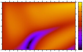
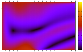
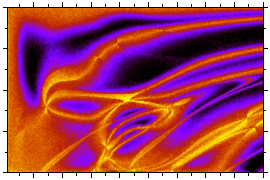
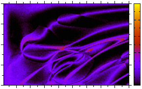
r1subscript𝑟1\phantom{\eta}r_{1}\phantom{\eta}Refer to caption-1-0.500.51

cosθc.m.subscript𝜃c.m.\cos\theta_{\text{c.m.}}

r2subscript𝑟2\phantom{\eta}r_{2}\phantom{\eta}Refer to caption00.20.40.60.81
r3subscript𝑟3\phantom{\eta}r_{3}\phantom{\eta}Refer to caption1.71.81.92.02.12.22.32.42.5W𝑊W(GeV)-1-0.500.51

cosθc.m.subscript𝜃c.m.\cos\theta_{\text{c.m.}}

r4subscript𝑟4\phantom{\eta}r_{4}\phantom{\eta}Refer to caption1.71.81.92.02.12.22.32.42.5W𝑊W(GeV)00.20.40.60.81
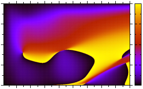
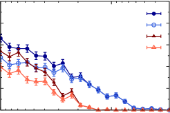
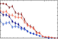
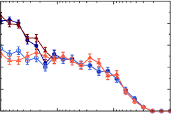
Figure 1: (Color online) The energy and angular dependence of the moduli risubscript𝑟𝑖r_{i} of the normalized transversity amplitudes for the γpK+Λ𝛾𝑝superscript𝐾Λ\gamma p\to K^{+}\Lambda reaction. The calculations are performed with the RPR-2011 model (ΔW2.38Δ𝑊2.38\Delta W\approx 2.38 MeV, Δcosθc.m.8.33×103Δsubscript𝜃c.m.8.33superscript103\Delta\cos\theta_{\text{c.m.}}\approx 8.33\times 10^{-3}).
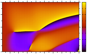
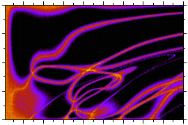
δ1subscript𝛿1\phantom{\eta}\delta_{1}\phantom{\eta}Refer to caption-1-0.500.51

cosθc.m.subscript𝜃c.m.\cos\theta_{\text{c.m.}}

00π2𝜋2\dfrac{\pi}{2}π𝜋\pi3π23𝜋2\dfrac{3\pi}{2}2π2𝜋2\pi
δ2subscript𝛿2\phantom{\eta}\delta_{2}\phantom{\eta}Refer to caption-1-0.500.51

cosθc.m.subscript𝜃c.m.\cos\theta_{\text{c.m.}}

00π2𝜋2\dfrac{\pi}{2}π𝜋\pi3π23𝜋2\dfrac{3\pi}{2}2π2𝜋2\pi
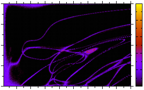
δ3subscript𝛿3\phantom{\eta}\delta_{3}\phantom{\eta}Refer to caption1.71.81.92.02.12.22.32.42.5W𝑊W(GeV)-1-0.500.51

cosθc.m.subscript𝜃c.m.\cos\theta_{\text{c.m.}}

00π2𝜋2\dfrac{\pi}{2}π𝜋\pi3π23𝜋2\dfrac{3\pi}{2}2π2𝜋2\pi
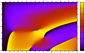
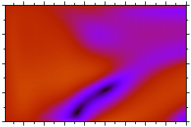
Figure 2: (Color online) The energy and angular dependence of the independent phases δisubscript𝛿𝑖\delta_{i} of the normalized transversity amplitudes of the γpK+Λ𝛾𝑝superscript𝐾Λ\gamma p\to K^{+}\Lambda reaction. The calculations are performed with the RPR-2011 model (ΔW1.43Δ𝑊1.43\Delta W\approx 1.43 MeV, Δcosθc.m.=5×10³Δsubscript𝜃c.m.5superscript103\Delta\cos\theta_{\text{c.m.}}=5\times 10^{-3}).

One would like to have a consistent set of estimators for the independent phases δiαjsuperscriptsubscript𝛿𝑖subscript𝛼𝑗\delta_{i}^{\;\alpha_{j}} (ij𝑖𝑗i\neq j) and δiα4δisuperscriptsubscript𝛿𝑖subscript𝛼4subscript𝛿𝑖\delta_{i}^{\;\alpha_{4}}\equiv\delta_{i} (i=1,2,3𝑖123i=1,2,3). The notation δ~iαjsuperscriptsubscript~𝛿𝑖subscript𝛼𝑗\widetilde{\delta}_{i}^{\;\alpha_{j}} is adopted for the consistent estimators. The aforementioned reference-phase ambiguity can be resolved by imposing that

δ~iαj=δ~iαkδ~jαk.superscriptsubscript~𝛿𝑖subscript𝛼𝑗superscriptsubscript~𝛿𝑖subscript𝛼𝑘superscriptsubscript~𝛿𝑗subscript𝛼𝑘\displaystyle\widetilde{\delta}_{i}^{\;\alpha_{j}}=\widetilde{\delta}_{i}^{\;\alpha_{k}}-\widetilde{\delta}_{j}^{\;\alpha_{k}}. (37)

Since this requirement is linear in the independent phases, the consistent estimators are also linear in {δ^iαl,δ^jαl,Δ^ik,Δ^jk}superscriptsubscript^𝛿𝑖subscript𝛼𝑙superscriptsubscript^𝛿𝑗subscript𝛼𝑙subscript^Δ𝑖𝑘subscript^Δ𝑗𝑘\{\widehat{\delta}_{i}^{\;\alpha_{l}},\widehat{\delta}_{j}^{\;\alpha_{l}},\widehat{\Delta}_{ik},\widehat{\Delta}_{jk}\} (ijkl)𝑖𝑗𝑘𝑙\left(i\neq j\neq k\neq l\right). The most general expression for a consistent set of estimated phases, reads

{δ~iαl=c1δ^iαl+(1c1)(δ^jαl+Δ^ikΔ^jk),δ~jαl=c1δ^jαl+(1c1)(δ^iαl+Δ^jkΔ^ik),δ~kαl=c2(δ^iαlΔ^ik)+(1c2)(δ^jαlΔ^jk).casessuperscriptsubscript~𝛿𝑖subscript𝛼𝑙subscript𝑐1superscriptsubscript^𝛿𝑖subscript𝛼𝑙1subscript𝑐1superscriptsubscript^𝛿𝑗subscript𝛼𝑙subscript^Δ𝑖𝑘subscript^Δ𝑗𝑘otherwisesuperscriptsubscript~𝛿𝑗subscript𝛼𝑙subscript𝑐1superscriptsubscript^𝛿𝑗subscript𝛼𝑙1subscript𝑐1superscriptsubscript^𝛿𝑖subscript𝛼𝑙subscript^Δ𝑗𝑘subscript^Δ𝑖𝑘otherwisesuperscriptsubscript~𝛿𝑘subscript𝛼𝑙subscript𝑐2superscriptsubscript^𝛿𝑖subscript𝛼𝑙subscript^Δ𝑖𝑘1subscript𝑐2superscriptsubscript^𝛿𝑗subscript𝛼𝑙subscript^Δ𝑗𝑘otherwise\displaystyle\begin{cases}\widetilde{\delta}_{i}^{\;\alpha_{l}}=c_{1}\widehat{\delta}_{i}^{\;\alpha_{l}}+(1-c_{1})\bigl{(}\widehat{\delta}_{j}^{\;\alpha_{l}}+\widehat{\Delta}_{ik}-\widehat{\Delta}_{jk}\bigr{)},\vspace{5pt}\\ \widetilde{\delta}_{j}^{\;\alpha_{l}}=c_{1}\widehat{\delta}_{j}^{\;\alpha_{l}}+(1-c_{1})\bigl{(}\widehat{\delta}_{i}^{\;\alpha_{l}}+\widehat{\Delta}_{jk}-\widehat{\Delta}_{ik}\bigr{)},\vspace{5pt}\\ \widetilde{\delta}_{k}^{\;\alpha_{l}}=c_{2}\bigl{(}\widehat{\delta}_{i}^{\;\alpha_{l}}-\widehat{\Delta}_{ik}\bigr{)}+(1-c_{2})\bigl{(}\widehat{\delta}_{j}^{\;\alpha_{l}}-\widehat{\Delta}_{jk}\bigr{)}.\end{cases} (38)

Here, three constraints have been imposed. Firstly, the δ~{i,j,k}αlsuperscriptsubscript~𝛿𝑖𝑗𝑘subscript𝛼𝑙\widetilde{\delta}_{\{i,j,k\}}^{\;\alpha_{l}} should yield the exact set δ{i,j,k}αlsuperscriptsubscript𝛿𝑖𝑗𝑘subscript𝛼𝑙\delta_{\{i,j,k\}}^{\;\alpha_{l}} for vanishing experimental error bars. Secondly, the expressions for δ~iαlsuperscriptsubscript~𝛿𝑖subscript𝛼𝑙\widetilde{\delta}_{i}^{\;\alpha_{l}} and δ~jαlsuperscriptsubscript~𝛿𝑗subscript𝛼𝑙\widetilde{\delta}_{j}^{\;\alpha_{l}} should be equal for ij𝑖𝑗i\leftrightarrow j. This leaves one with two unknowns c1subscript𝑐1c_{1} and c2subscript𝑐2c_{2}. Thirdly, c1subscript𝑐1c_{1} and c2subscript𝑐2c_{2} cannot depend on αlsubscript𝛼𝑙\alpha_{l}, which is implied by Eq. (37). By applying Eq. (37) on expressions (38) and by using Table 2, one readily finds that c1=34subscript𝑐134c_{1}=\frac{3}{4} and c2=12subscript𝑐212c_{2}=\frac{1}{2}. Therefore, the consistent set of estimators for the phases, reads

{δ~iαl=34δ^iαl+14(δ^jαl+Δ^ikΔ^jk),δ~jαl=34δ^jαl+14(δ^iαl+Δ^jkΔ^ik),δ~kαl=12(δ^iαlΔ^ik)+12(δ^jαlΔ^jk).casessuperscriptsubscript~𝛿𝑖subscript𝛼𝑙34superscriptsubscript^𝛿𝑖subscript𝛼𝑙14superscriptsubscript^𝛿𝑗subscript𝛼𝑙subscript^Δ𝑖𝑘subscript^Δ𝑗𝑘otherwisesuperscriptsubscript~𝛿𝑗subscript𝛼𝑙34superscriptsubscript^𝛿𝑗subscript𝛼𝑙14superscriptsubscript^𝛿𝑖subscript𝛼𝑙subscript^Δ𝑗𝑘subscript^Δ𝑖𝑘otherwisesuperscriptsubscript~𝛿𝑘subscript𝛼𝑙12superscriptsubscript^𝛿𝑖subscript𝛼𝑙subscript^Δ𝑖𝑘12superscriptsubscript^𝛿𝑗subscript𝛼𝑙subscript^Δ𝑗𝑘otherwise\displaystyle\begin{cases}\widetilde{\delta}_{i}^{\;\alpha_{l}}=\frac{3}{4}\widehat{\delta}_{i}^{\;\alpha_{l}}+\frac{1}{4}\bigl{(}\widehat{\delta}_{j}^{\;\alpha_{l}}+\widehat{\Delta}_{ik}-\widehat{\Delta}_{jk}\bigr{)},\vspace{5pt}\\ \widetilde{\delta}_{j}^{\;\alpha_{l}}=\frac{3}{4}\widehat{\delta}_{j}^{\;\alpha_{l}}+\frac{1}{4}\bigl{(}\widehat{\delta}_{i}^{\;\alpha_{l}}+\widehat{\Delta}_{jk}-\widehat{\Delta}_{ik}\bigr{)},\vspace{5pt}\\ \widetilde{\delta}_{k}^{\;\alpha_{l}}=\frac{1}{2}\bigl{(}\widehat{\delta}_{i}^{\;\alpha_{l}}-\widehat{\Delta}_{ik}\bigr{)}+\frac{1}{2}\bigl{(}\widehat{\delta}_{j}^{\;\alpha_{l}}-\widehat{\Delta}_{jk}\bigr{)}.\end{cases} (39)

The estimates δ~isubscript~𝛿𝑖\widetilde{\delta}_{i}’s (i=1,2,3𝑖123i=1,2,3) for the independent phases are now insensitive to the choices made with regard to the reference phase.

IV Results

IV.1 The angular and energy dependence of the transversity amplitudes

A complete measurement comprises a minimal set of asymmetries from which the accessible parameters of the normalized transversity amplitudes aisubscript𝑎𝑖a_{i} can be estimated. These parameters include three independent moduli risubscript𝑟𝑖r_{i} and three independent relative phases δisubscript𝛿𝑖\delta_{i}. In Sec. III, it was shown how the moduli can be obtained from the single asymmetries and how a set of three independent phases can be estimated in a consistent way from a complete measurement which also involves double asymmetries.

Figures 1 and 2 show the (W𝑊W, cosθc.m.subscript𝜃c.m.\cos\theta_{\text{c.m.}}) dependence of the risubscript𝑟𝑖r_{i} and the δisubscript𝛿𝑖\delta_{i} for the γpK+Λ𝛾𝑝superscript𝐾Λ\gamma p\to K^{+}\Lambda reaction as predicted by a realistic model, namely the latest version of the Regge-plus-Resonance (RPR) model, i.e. RPR-2011 tamaraprc ; lesleyprl ; lesleyprc . This model has a Reggeized t𝑡t-channel background and includes a total of 8 s𝑠s-channel resonances, namely S11(1535)subscript𝑆111535S_{11}(1535), S11(1650)subscript𝑆111650S_{11}(1650), F15(1680)subscript𝐹151680F_{15}(1680), P13(1720)subscript𝑃131720P_{13}(1720), P11(1900)subscript𝑃111900P_{11}(1900), P13(1900)subscript𝑃131900P_{13}(1900), D13(1900)subscript𝐷131900D_{13}(1900), and F15(2000)subscript𝐹152000F_{15}(2000). The most apparent feature of the RPR-2011 predictions for the moduli and phases are the strong variations with energy W𝑊W at backward scattering angles, due to s𝑠s-channel resonances. The smooth energy dependence of the moduli and phases at very forward scattering angles reflects the important t𝑡t-channel background contributions of γpK+Λ𝛾𝑝superscript𝐾Λ\gamma p\to K^{+}\Lambda. At forward kaon angles, where most of the strength resides, the RPR-2011 model predicts a dominant role for r2subscript𝑟2r_{2}.

00.20.40.60.8

r1subscript𝑟1r_{1}

0.808cosθc.m.0.861less-than-or-similar-to0.808subscript𝜃c.m.less-than-or-similar-to0.8610.808\lesssim\cos\theta_{\text{c.m.}}\lesssim 0.861Refer to captionRPR-2011 GRAAL 
00.20.40.145cosθc.m.0.173less-than-or-similar-to0.145subscript𝜃c.m.less-than-or-similar-to0.1730.145\lesssim\cos\theta_{\text{c.m.}}\lesssim 0.173Refer to caption
0.20.40.60.80.806cosθc.m.0.750less-than-or-similar-to0.806subscript𝜃c.m.less-than-or-similar-to0.750-0.806\lesssim\cos\theta_{\text{c.m.}}\lesssim-0.750Refer to caption


          0.60.70.80.9

r2subscript𝑟2r_{2}

Refer to caption
         0.60.70.80.9Refer to caption         00.20.40.60.8Refer to caption

          0.40.50.6

r3subscript𝑟3r_{3}

Refer to caption
         0.40.50.60.7Refer to caption         0.20.40.60.8Refer to caption

          00.20.40.61.651.701.751.801.851.90

r4subscript𝑟4r_{4}

W𝑊W(GeV)Refer to caption
         0.10.20.30.40.51.651.701.751.801.851.90W𝑊W(GeV)Refer to caption         0.20.40.61.651.701.751.801.851.90W𝑊W(GeV)Refer to caption


Figure 3: (Color online) The energy dependence of the moduli risubscript𝑟𝑖r_{i} of the normalized transversity amplitudes for the γpK+Λ𝛾𝑝superscript𝐾Λ\gamma p\to K^{+}\Lambda reaction. The data are extracted from the GRAAL results for the single-polarization observables reported in Refs. Lleres2007 ; Lleres2009 . The dots are the bin-centered RPR-2011 predictions.

IV.2 The merits of the transversity basis

In Sec. III, it was shown how the transversity amplitudes can be inferred from a complete set of measured observables. The first and essential step comprised the determination of the moduli from the three single asymmetries. Indeed, as became clear, the extraction of the δisubscript𝛿𝑖\delta_{i} requires prior knowledge about the moduli risubscript𝑟𝑖r_{i}. Luckily enough, single asymmetries are more easily obtained experimentally than double asymmetries. Consequently, the single asymmetries database generally have better statistics compared to double polarization observables. The published database for e.g. γpK+Λ𝛾𝑝superscript𝐾Λ\gamma p\to K^{+}\Lambda includes 2260 single asymmetries (ΣΣ\Sigma: 178, T𝑇T: 69, P𝑃P: 2013), in contrast to only 456 double asymmetries (Cxsubscript𝐶𝑥C_{x}: 162, Czsubscript𝐶𝑧C_{z}: 162, Oxsubscript𝑂superscript𝑥O_{x^{\prime}}: 66, Ozsubscript𝑂superscript𝑧O_{z^{\prime}}: 66) lesleyprc . The beam-recoil asymmetries {Ox,Oz}subscript𝑂superscript𝑥subscript𝑂superscript𝑧\{O_{x^{\prime}},O_{z^{\prime}}\} are related to {Ox,Oz}subscript𝑂𝑥subscript𝑂𝑧\{O_{x},O_{z}\} through Eq. (50). In the transversity representation the parameters that are most easily extracted from the data, namely the moduli, are related to that class of asymmetries that are more readily measured, namely the single asymmetries. This is not the case for the helicity basis, where the moduli are related to the set of double asymmetries {Cz,E,Lz}subscript𝐶superscript𝑧𝐸subscript𝐿superscript𝑧\{C_{z^{\prime}},E,L_{z^{\prime}}\}. It is important to stress that determining invariant amplitudes at some kinematical point requires knowledge of a complete set at the same kinematics. To date, however, there is not a single pseudoscalar photoproduction reaction for which a complete dataset has been published.

For the γpK+Λ𝛾𝑝superscript𝐾Λ\gamma p\to K^{+}\Lambda reaction, the GRAAL collaboration has measured {Σ,T,P}Σ𝑇𝑃\{\Sigma,T,P\} at 66 kinematical points Lleres2007 ; Lleres2009 . These data cover 1.65W1.91less-than-or-similar-to1.65𝑊less-than-or-similar-to1.911.65\lesssim W\lesssim 1.91 GeV (bins of ΔW50Δ𝑊50\Delta W\approx 50 MeV) and 0.81cosθc.m.0.86less-than-or-similar-to0.81subscript𝜃c.m.less-than-or-similar-to0.86-0.81\lesssim\cos\theta_{\text{c.m.}}\lesssim 0.86 (bins of Δcosθc.m.0.3Δsubscript𝜃c.m.0.3\Delta\cos\theta_{\text{c.m.}}\approx 0.3), and can be used to estimate the moduli risubscript𝑟𝑖r_{i} through Eqs. (27). Figure 3 shows these extracted moduli at three cosθc.m.subscript𝜃c.m.\cos\theta_{\text{c.m.}} intervals (33 of the 66 kinematical points for which data is available) along with the corresponding predictions from RPR-2011. It is observed that at a few kinematical points, some of the r^isubscript^𝑟𝑖\widehat{r}_{i} cannot be extracted from the data. This occurs whenever the measured set {Σ,T,P}Σ𝑇𝑃\{\Sigma,T,P\} deviates too strongly from the ‘exact’ set so that one or more arguments of the square roots (27) become negative. For the GRAAL data, only 17 of the 66×4=26466426466\times 4=264 r^isubscript^𝑟𝑖\widehat{r}_{i} values are imaginary (r1subscript𝑟1r_{1}: 12, r2subscript𝑟2r_{2}: 3, r4subscript𝑟4r_{4}: 2). Overall, the RPR-2011 model offers a fair description of the energy and angular dependence of the extracted r^isubscript^𝑟𝑖\widehat{r}_{i} except for the r^2subscript^𝑟2\widehat{r}_{2} and r^4subscript^𝑟4\widehat{r}_{4} at 0.808cosθc.m.0.861less-than-or-similar-to0.808subscript𝜃c.m.less-than-or-similar-to0.8610.808\lesssim\cos\theta_{\text{c.m.}}\lesssim 0.861.

Obviously, the GRAAL bin width of ΔW50Δ𝑊50\Delta W\approx 50 MeV suffices to map the energy dependence of the risubscript𝑟𝑖r_{i}. The most extensive γpK+Λ𝛾𝑝superscript𝐾Λ\gamma p\to K^{+}\Lambda data set to date is due to the CLAS collaboration at Jefferson Lab cracken2010 . The data cover 1.62W2.841.62𝑊2.841.62\leq W\leq 2.84 GeV (bins of ΔW=10Δ𝑊10\Delta W=10 MeV) and 0.85cosθc.m.0.950.85subscript𝜃c.m.0.95-0.85\leq\cos\theta_{\text{c.m.}}\leq 0.95 (bins of Δcosθc.m.=0.1Δsubscript𝜃c.m.0.1\Delta\cos\theta_{\text{c.m.}}=0.1) and include data for dσdΩd𝜎dΩ\frac{\mathrm{d}\sigma}{\mathrm{d}\Omega} and the recoil polarization P𝑃P.

In addition to {Σ,T,P}Σ𝑇𝑃\{\Sigma,T,P\}, GRAAL provides data for {Ox,Oz}subscript𝑂superscript𝑥subscript𝑂superscript𝑧\{O_{x^{\prime}},O_{z^{\prime}}\} at the same kinematical points. Since a complete set of asymmetries is required to extract the δisubscript𝛿𝑖\delta_{i}, these beam-recoil data cannot be employed in order to gain additional information about the transversity amplitudes.

As is seen from Table 8, the GRAAL data for {Σ,T,P,Ox,Oz}Σ𝑇𝑃subscript𝑂superscript𝑥subscript𝑂superscript𝑧\{\Sigma,T,P,O_{x^{\prime}},O_{z^{\prime}}\} cannot be used to extract the moduli of the helicity amplitudes. The latter would require experimental data for {Cz,E,Lz}subscript𝐶superscript𝑧𝐸subscript𝐿superscript𝑧\{C_{z^{\prime}},E,L_{z^{\prime}}\} at the same kinematics, which is not available to this day. Clearly, given the current status of the experimental γpK+Λ𝛾𝑝superscript𝐾Λ\gamma p\to K^{+}\Lambda program, the transversity representation offers the best perspectives to learn about the reaction amplitudes.

The extracted information about the energy and angular dependence of the amplitudes ri(W,cosθc.m.)subscript𝑟𝑖𝑊subscript𝜃c.m.r_{i}(W,\cos\theta_{\text{c.m.}}) of Fig. 3 is complementary to what could be obtained about the partial waves in a so-called truncated partial wave analysis (TPWA) Tiator:2012ah ; Tiator:2011tu ; Workman:2011hi . In TPWA one aims at extracting information about the energy dependence of the partial waves from the experimental data. The partial waves serve as expansion parameters for the angular dependence of the observables. The amount of partial waves which can be included (usually denoted by lmaxsubscript𝑙l_{\max}) in the fits, depends on the quality and quantity of the measured cosθc.m.subscript𝜃c.m.\cos\theta_{\text{c.m.}} dependence of the observables. It is anticipated that in a reaction channel like γpK+Λ𝛾𝑝superscript𝐾Λ\gamma p\to K^{+}\Lambda with substantial background contributions, lmaxsubscript𝑙l_{\max} cannot be truncated to small values. In the TPWA approach the underlying dynamics is parameterized in terms of functions which depend on W𝑊W, whereas in an amplitude analysis as presented here, one attempts to map the full (W,cosθc.m.)𝑊subscript𝜃c.m.(W,\cos\theta_{\text{c.m.}}) dependence. In the forthcoming section, it will be shown that the availability of complete sets of eight observables with realistic error bars at given (W,cosθc.m.)𝑊subscript𝜃c.m.(W,\cos\theta_{\text{c.m.}}) does not guarantee that one can retrieve the underlying transversity amplitudes. In a recent analysis of γNπN𝛾𝑁𝜋𝑁\gamma N\to\pi N simulated data Workman:2011hi it was shown that the availability of the cosθc.m.subscript𝜃c.m.\cos\theta_{\text{c.m.}} dependence of six observables at given W𝑊W yields unique partial-wave solutions.

IV.3 Extracting the transversity amplitudes from RPR-2011 simulations

In this section the completeness of complete sets is investigated. The analysis is performed for the representative complete set {Cx,Ox,E,F}subscript𝐶𝑥subscript𝑂𝑥𝐸𝐹\{C_{x},O_{x},E,F\} of the first kind. The goal is to determine the moduli r^isubscript^𝑟𝑖\widehat{r}_{i} and the consistent independent phases δ~isubscript~𝛿𝑖\widetilde{\delta}_{i} of the transversity amplitudes from simulated observables with finite experimental resolution generated with the RPR-2011 model. It is investigated to what extent the retrieved amplitudes comply with the input amplitudes from the simulations.

IV.3.1 Strategy

A measured asymmetry is simulated by generating a fixed number of events from a Gaussian distribution. The mean of this distribution is the RPR-2011 prediction for a certain value of W𝑊W and cosθc.m.subscript𝜃c.m.\cos\theta_{\text{c.m.}}. The standard deviation is a specific experimental resolution σexpsubscript𝜎exp\sigma_{\text{exp}}. The mean and standard deviation of the generated events determine the value and the error of the simulated data point. If the error of the simulated data point is smaller than the specified σexpsubscript𝜎exp\sigma_{\text{exp}}, the former is rejected.

From a simulated set {Cx,Ox,\{C_{x},O_{x},E,F}E,F\}, one can obtain the r^isubscript^𝑟𝑖\widehat{r}_{i} and the δ~isubscript~𝛿𝑖\widetilde{\delta}_{i} by means of Eqs. (27) and (39). In order to estimate the error on the r^isubscript^𝑟𝑖\widehat{r}_{i} and the δ~isubscript~𝛿𝑖\widetilde{\delta}_{i}, standard error propagation is applied. Since seven asymmetries are required to estimate the six parameters of the normalized transversity amplitudes, the correlation between the asymmetries has to be taken into account upon estimating errors. The squared error of a certain function f𝑓f of the asymmetries is calculated as

σ2(f)=i(fAi)2σ2(Ai)+i,jijfAifAjσ(Ai,Aj),superscript𝜎2𝑓subscript𝑖superscript𝑓subscript𝐴𝑖2superscript𝜎2subscript𝐴𝑖subscript𝑖𝑗𝑖𝑗𝑓subscript𝐴𝑖𝑓subscript𝐴𝑗𝜎subscript𝐴𝑖subscript𝐴𝑗\sigma^{2}(f)=\sum_{i}\left(\frac{\partial f}{\partial A_{i}}\right)^{2}\sigma^{2}(A_{i})\\ +\sum_{\begin{subarray}{c}i,j\\ i\neq j\end{subarray}}\frac{\partial f}{\partial A_{i}}\frac{\partial f}{\partial A_{j}}\sigma(A_{i},A_{j}), (40)

with Ai,Aj{Σ,T,P,Cx,Ox,E,F}subscript𝐴𝑖subscript𝐴𝑗Σ𝑇𝑃subscript𝐶𝑥subscript𝑂𝑥𝐸𝐹A_{i},A_{j}\in\{\Sigma,T,P,C_{x},O_{x},E,F\} and σ(Ai,Aj)𝜎subscript𝐴𝑖subscript𝐴𝑗\sigma(A_{i},A_{j}) the covariance between Aisubscript𝐴𝑖A_{i} and Ajsubscript𝐴𝑗A_{j}.

IV.3.2 Analysis

As indicated in Sec. IV.2, the extraction of the r^isubscript^𝑟𝑖\widehat{r}_{i} from a measured set of single asymmetries through Eqs. (27) is rather straightforward. In some isolated situations at least one of the retrieved r^isubscript^𝑟𝑖\widehat{r}_{i} became imaginary. The moduli estimates, however, are required to extract the relevant phases from a complete set, as is seen from Eqs. (29), (30), and (32). Consequently, an imaginary estimate for one of the moduli results in imaginary estimates for the phases, no matter the achieved precision of the double-asymmetry observables. Through the normalization condition (18) only three of the four moduli are independent. One imaginary modulus estimate, be it an independent or a nonindependent one, is sufficient to jeopardize the phase analysis. For this reason, the four moduli are treated on equal grounds and a selection of a set of three independent moduli has been avoided all along.

Table 3: The model’s values and two simulated datasets for the complete set {Cx,Ox,E,F}subscript𝐶𝑥subscript𝑂𝑥𝐸𝐹\{C_{x},O_{x},E,F\} at W=1700𝑊1700W=1700 MeV and cosθc.m.=0.5subscript𝜃c.m.0.5\cos\theta_{\text{c.m.}}=-0.5 with σexp=0.05subscript𝜎exp0.05\sigma_{\text{exp}}=0.05.
Model Simulation A Simulation B
ΣΣ\Sigma 0.04890.0489\phantom{-}0.0489 0.0543±0.0519plus-or-minus0.05430.0519\phantom{-}0.0543\pm 0.0519 0.0458±0.0533plus-or-minus0.04580.0533\phantom{-}0.0458\pm 0.0533
T𝑇T 0.68430.6843-0.6843 0.6905±0.0511plus-or-minus0.69050.0511-0.6905\pm 0.0511 0.6685±0.0524plus-or-minus0.66850.0524-0.6685\pm 0.0524
P𝑃P 0.00560.0056\phantom{-}0.0056 0.0111±0.0552plus-or-minus0.01110.0552\phantom{-}0.0111\pm 0.0552 0.0892±0.0555plus-or-minus0.08920.0555\phantom{-}0.0892\pm 0.0555
Cxsubscript𝐶𝑥C_{x} 0.48080.4808-0.4808 0.4809±0.0515plus-or-minus0.48090.0515-0.4809\pm 0.0515 0.4728±0.0588plus-or-minus0.47280.0588-0.4728\pm 0.0588
Oxsubscript𝑂𝑥O_{x} 0.59890.5989-0.5989 0.5971±0.0519plus-or-minus0.59710.0519-0.5971\pm 0.0519 0.6149±0.0567plus-or-minus0.61490.0567-0.6149\pm 0.0567
E𝐸E 0.56720.5672\phantom{-}0.5672 0.5655±0.0505plus-or-minus0.56550.0505\phantom{-}0.5655\pm 0.0505 0.5695±0.0564plus-or-minus0.56950.0564\phantom{-}0.5695\pm 0.0564
F𝐹F 0.45250.4525-0.4525 0.4411±0.0519plus-or-minus0.44110.0519-0.4411\pm 0.0519 0.4486±0.0503plus-or-minus0.44860.0503-0.4486\pm 0.0503
Table 4: The model’s values for the r^isubscript^𝑟𝑖\widehat{r}_{i} at W=1700𝑊1700W=1700 MeV and cosθc.m.=0.5subscript𝜃c.m.0.5\cos\theta_{\text{c.m.}}=-0.5, and the corresponding estimates from dataset A and dataset B.
Model Simulation A Simulation B
r^1subscript^𝑟1\widehat{r}_{1} 0.3040.3040.304 0.306±0.037plus-or-minus0.3060.0370.306\pm 0.037 0.311±0.037plus-or-minus0.3110.0370.311\pm 0.037
r^2subscript^𝑟2\widehat{r}_{2} 0.6570.6570.657 0.658±0.017plus-or-minus0.6580.0170.658\pm 0.017 0.653±0.018plus-or-minus0.6530.0180.653\pm 0.018
r^3subscript^𝑟3\widehat{r}_{3} 0.6400.6400.640 0.642±0.018plus-or-minus0.6420.0180.642\pm 0.018 0.639±0.018plus-or-minus0.6390.0180.639\pm 0.018
r^4subscript^𝑟4\widehat{r}_{4} 0.2560.2560.256 0.248±0.046plus-or-minus0.2480.0460.248\pm 0.046 0.263±0.044plus-or-minus0.2630.0440.263\pm 0.044
Table 5: The constraint of Eq. (31) for the four {δ1,δ2,Δ13,Δ23}subscript𝛿1subscript𝛿2subscriptΔ13subscriptΔ23\{\delta_{1},\delta_{2},\Delta_{13},\Delta_{23}\} solutions extracted from the simulated data listed in Table 3. The number of standard deviations, by which the constraint differs from zero, is denoted by nσsubscript𝑛𝜎n_{\sigma}. The ci are the confidence intervals corresponding with the nσsubscript𝑛𝜎n_{\sigma}.
Solution Simulation A
Constraint nσsubscript𝑛𝜎n_{\sigma} ci (%)
111 0.029±3.866plus-or-minus0.0293.866\phantom{-}0.029\pm 3.866 0.0070.0070.007 99.499.499.4
222 0.200±3.316plus-or-minus0.2003.316-0.200\pm 3.316 0.0600.0600.060 95.295.295.2
333 2.513±3.316plus-or-minus2.5133.316-2.513\pm 3.316 0.7580.7580.758 44.944.944.9
444 2.741±3.865plus-or-minus2.7413.865-2.741\pm 3.865 0.7090.7090.709 47.847.847.8


Solution Simulation B Constraint nσsubscript𝑛𝜎n_{\sigma} ci (%) 111 0.592±1.261plus-or-minus0.5921.261\phantom{-}0.592\pm 1.261 0.4670.4670.467 63.863.863.8 222 0.229±0.898plus-or-minus0.2290.898-0.229\pm 0.898 0.2550.2550.255 79.979.979.9 333 2.393±0.903plus-or-minus2.3930.903-2.393\pm 0.903 2.6512.6512.651 0.80.8\phantom{0}0.8 444 3.069±1.264plus-or-minus3.0691.264\phantom{-}3.069\pm 1.264 2.4282.4282.428 1.51.5\phantom{0}1.5

Estimating the δisubscript𝛿𝑖\delta_{i} is far less straightforward than estimating the risubscript𝑟𝑖r_{i}. Table 3 lists two simulated measurements of the complete set {Cx,Ox,E,F}subscript𝐶𝑥subscript𝑂𝑥𝐸𝐹\{C_{x},O_{x},E,F\} at W=1700𝑊1700W=1700 MeV and cosθc.m.=0.5subscript𝜃c.m.0.5\cos\theta_{\text{c.m.}}=-0.5, performed at an input resolution of σexp=0.05subscript𝜎exp0.05\sigma_{\text{exp}}=0.05. The mean value and standard deviation of the asymmetries were calculated from a sample of 50 events. Upon inspecting Table 3, both simulations are seen to be qualitatively equivalent. This is also reflected by the accurate moduli estimates from both simulations, which are listed in Table 4. In Sec. III.2.2 it was mentioned that four distinct solutions for {δ1,δ2,Δ13,Δ23}subscript𝛿1subscript𝛿2subscriptΔ13subscriptΔ23\{\delta_{1},\delta_{2},\Delta_{13},\Delta_{23}\} exist for the concerned complete set. Only one satisfies the constraint (31) in the exact case, though. When experimental error is involved, however, none of the four solutions satisfies the constraint. In Table 5, the outcome of constraint (31) is listed for each of the four solutions to both datasets. As the constraint is a sum of phases and its evaluation in the exact case yields a zero value, the mean values listed in Table 5 were rotated to ]π,+π]]-\pi,+\pi]. The table also lists by how many standard deviations (denoted by nσsubscript𝑛𝜎n_{\sigma}) the mean deviates from zero. The solution with the lowest nσsubscript𝑛𝜎n_{\sigma} has the highest likelihood. In principle a solution can be excluded if it is statistically insignificant, commonly quantified by a small confidence interval ci=1erf(nσ/2)ci1erfsubscript𝑛𝜎2\textsc{ci}=1-\text{erf}\left(n_{\sigma}/\sqrt{2}\right). From the ci values of dataset B it follows that solution 3 and solution 4 can be excluded with significance. For dataset A, these solutions are also the least significant ones. Of the two remaining solutions, dataset A predicts that solution 1 is the real solution (99.4%percent99.499.4\% ci). According to dataset B, however, solution 2 is the most likely one, though with a smaller confidence interval (79.9%percent79.979.9\% ci). This example illustrates that ambiguities remain for (theoretically) complete sets when experimental uncertainties are taken into account.

Table 6: The model’s values for the δ~isubscript~𝛿𝑖\widetilde{\delta}_{i} at W=1700𝑊1700W=1700 MeV and cosθc.m.=0.5subscript𝜃c.m.0.5\cos\theta_{\text{c.m.}}=-0.5, along with the estimates resulting from the most significant solution of dataset A (solution 1) and dataset B (solution 2).
Model Simulation A Simulation B
δ~1subscript~𝛿1\widetilde{\delta}_{1} 0.4870.4870.487 0.424±0.801plus-or-minus0.4240.8010.424\pm 0.801 0.704±0.478plus-or-minus0.7040.4780.704\pm 0.478
δ~2subscript~𝛿2\widetilde{\delta}_{2} 2.4582.4582.458 2.424±0.992plus-or-minus2.4240.9922.424\pm 0.992 2.637±0.348plus-or-minus2.6370.3482.637\pm 0.348
δ~3subscript~𝛿3\widetilde{\delta}_{3} 6.1066.1066.106 6.090±0.235plus-or-minus6.0900.2356.090\pm 0.235 3.046±0.234plus-or-minus3.0460.2343.046\pm 0.234
00.20.40.60.810.010.1

η𝜂\eta

W=1700𝑊1700W=1700MeVcosθc.m.=0.9subscript𝜃c.m.0.9\cos\theta_{\text{c.m.}}=0.9Refer to captionη𝜂\eta{Cx,Ox,E,F}subscript𝐶𝑥subscript𝑂𝑥𝐸𝐹\{C_{x},O_{x},E,F\}ηimaginarysubscript𝜂imaginary\eta_{\text{imaginary}}{Cx,Ox,E,F}subscript𝐶𝑥subscript𝑂𝑥𝐸𝐹\{C_{x},O_{x},E,F\}η𝜂\eta{Cx,Ox,G,H}subscript𝐶𝑥subscript𝑂𝑥𝐺𝐻\{C_{x},O_{x},G,H\}ηimaginarysubscript𝜂imaginary\eta_{\text{imaginary}}{Cx,Ox,G,H}subscript𝐶𝑥subscript𝑂𝑥𝐺𝐻\{C_{x},O_{x},G,H\}
0.010.1W=1800𝑊1800W=1800MeVcosθc.m.=0subscript𝜃c.m.0\cos\theta_{\text{c.m.}}=0Refer to caption


00.20.40.60.810.00010.0010.010.1

η𝜂\eta

σexpsubscript𝜎exp\sigma_{\text{exp}}W=1800𝑊1800W=1800MeVcosθc.m.=0.3subscript𝜃c.m.0.3\cos\theta_{\text{c.m.}}=-0.3Refer to caption
         0.00010.0010.010.1σexpsubscript𝜎exp\sigma_{\text{exp}}W=2200𝑊2200W=2200MeVcosθc.m.=0.9subscript𝜃c.m.0.9\cos\theta_{\text{c.m.}}=-0.9Refer to caption


Figure 4: (Color online) The insolvability of the transversity amplitudes at four different kinematical points. The circles and triangles are simulated data generated from the complete sets {Cx,Ox,E,F}subscript𝐶𝑥subscript𝑂𝑥𝐸𝐹\{C_{x},O_{x},E,F\} and {Cx,Ox,G,H}subscript𝐶𝑥subscript𝑂𝑥𝐺𝐻\{C_{x},O_{x},G,H\}. The filled and unfilled symbols correspond with η=ηimaginary+ηincorrect𝜂subscript𝜂imaginarysubscript𝜂incorrect\eta=\eta_{\text{imaginary}}+\eta_{\text{incorrect}} and ηimaginarysubscript𝜂imaginary\eta_{\text{imaginary}}.
η(σexp=0.1)𝜂subscript𝜎exp0.1\eta\;(\sigma_{\text{exp}}=0.1)Refer to caption-1-0.500.51

cosθc.m.subscript𝜃c.m.\cos\theta_{\text{c.m.}}

ηincorrectsubscript𝜂incorrect\eta_{\text{incorrect}}(σexpsubscript𝜎exp\sigma_{\text{exp}} = 0.1)Refer to caption00.20.40.60.81
η(σexp=0.01)𝜂subscript𝜎exp0.01\eta\;(\sigma_{\text{exp}}=0.01)Refer to caption1.71.81.92.02.12.22.32.42.5W𝑊W(GeV)-1-0.500.51

cosθc.m.subscript𝜃c.m.\cos\theta_{\text{c.m.}}

ηincorrectsubscript𝜂incorrect\eta_{\text{incorrect}}(σexpsubscript𝜎exp\sigma_{\text{exp}} = 0.01)Refer to caption1.71.81.92.02.12.22.32.42.5W𝑊W(GeV)00.20.40.60.81
Figure 5: (Color online) The {Cx,Ox,E,F}subscript𝐶𝑥subscript𝑂𝑥𝐸𝐹\{C_{x},O_{x},E,F\} insolvabilities η=ηimaginary+ηincorrect𝜂subscript𝜂imaginarysubscript𝜂incorrect\eta=\eta_{\text{imaginary}}+\eta_{\text{incorrect}} and ηincorrectsubscript𝜂incorrect\eta_{\text{incorrect}} as a function of W𝑊W and cosθc.m.subscript𝜃c.m.\cos\theta_{\text{c.m.}} for two values of the input experimental resolution (σexp=0.1subscript𝜎exp0.1\sigma_{\text{exp}}=0.1 and σexp=0.01subscript𝜎exp0.01\sigma_{\text{exp}}=0.01).

In Table 6, the model’s phases are compared with the corresponding estimates from solution 1 of dataset A and solution 2 of dataset B. From this table, it is seen that solution 1 is the actual solution. This finding could have been anticipated by comparing ci values (99.4%percent99.499.4\% versus 79.9%percent79.979.9\%). However, a real experiment only yields a single dataset at a certain kinematical point. If an experiment were to yield dataset A, one could not exclude solutions 3 and 4 with significance and one could only conclude that solution 1 is most likely the real solution with 99.4%percent99.499.4\% ci. If dataset B were the result of a real experiment, then solutions 3 and 4 could be excluded with significance and one could state that solution 2 is most likely the actual solution with a ci value of only 79.9%percent79.979.9\%, though. The confidence interval on the constraint (31) is the only parameter able to distinguish between the four solutions. In some cases, however, the solution with the highest ci does not deliver the correct solution for the phases.

In the beginning of this section, it was argued that an imaginary estimate for the r^isubscript^𝑟𝑖\widehat{r}_{i} leads to imaginary δ~isubscript~𝛿𝑖\widetilde{\delta}_{i}. Even with real r^isubscript^𝑟𝑖\widehat{r}_{i}, however, it cannot be excluded that imaginary δ~isubscript~𝛿𝑖\widetilde{\delta}_{i} are retrieved. Indeed, from Eqs. (29) and (30) the phases are determined by solving a quadratic equation in the sine or cosine of the phase. For certain combinations of the measured double asymetries the discriminant of this quadratic equation becomes negative. In such case, the particular dataset can solely be used to estimate the moduli. In what follows the authors wish to quantify the insolvability of a complete set, i.e. how frequently it occurs that imaginary or incorrect solutions are obtained for the transversity amplitudes.

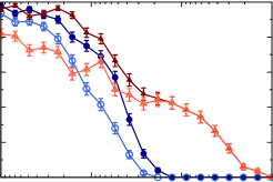
Figure 4 shows the insolvability of the transversity amplitudes as a function of the input experimental resolution σexpsubscript𝜎exp\sigma_{\text{exp}}. Simulations for the complete sets {Cx,Ox,E,F}subscript𝐶𝑥subscript𝑂𝑥𝐸𝐹\{C_{x},O_{x},E,F\} and {Cx,Ox,G,H}subscript𝐶𝑥subscript𝑂𝑥𝐺𝐻\{C_{x},O_{x},G,H\} are analyzed at four different kinematics. Each point in Fig. 4 results from an ensemble of 200 simulated datasets constructed from samples of 50 events for each of the asymmetries. The insolvability η𝜂\eta is the fraction of unsuccessful simulated datasets. The η𝜂\eta is defined as the sum of the fraction of (two or four) imaginary solutions (ηimaginarysubscript𝜂imaginary\eta_{\text{imaginary}}) and the fraction of incorrect solutions (ηincorrectsubscript𝜂incorrect\eta_{\text{incorrect}}). An incorrect solution is a solution with the highest ci value that does not correspond with the model’s value in the limit σexp0subscript𝜎exp0\sigma_{\text{exp}}\to 0. The insolvability η𝜂\eta is binomially distributed and hence the corresponding error is calculated as

σ(η)=η(1η)N,𝜎𝜂𝜂1𝜂𝑁\displaystyle\sigma(\eta)=\sqrt{\frac{\eta(1-\eta)}{N}}, (41)

where N𝑁N represents the number of simulated datasets. It is seen that the insolvability decreases with decreasing σexpsubscript𝜎exp\sigma_{\text{exp}}, as is expected. Further, the ηimaginarysubscript𝜂imaginary\eta_{\text{imaginary}} has the largest contribution and ηincorrectsubscript𝜂incorrect\eta_{\text{incorrect}} vanishes more rapidly with σexpsubscript𝜎exp\sigma_{\text{exp}} than ηimaginarysubscript𝜂imaginary\eta_{\text{imaginary}}. In some situations, the insolvability only vanishes for very challenging experimental resolutions, and it is seen that this behavior depends on the complete set in question.

Figure 5 shows the {Cx,Ox,E,F}subscript𝐶𝑥subscript𝑂𝑥𝐸𝐹\{C_{x},O_{x},E,F\} insolvabilities η𝜂\eta and ηincorrectsubscript𝜂incorrect\eta_{\text{incorrect}} as a function of W𝑊W and cosθc.m.subscript𝜃c.m.\cos\theta_{\text{c.m.}} for σexp=0.1subscript𝜎exp0.1\sigma_{\text{exp}}=0.1 and σexp=0.01subscript𝜎exp0.01\sigma_{\text{exp}}=0.01. For each of the 375×241=90 37537524190375375\times 241=90\,375 kinematical points, 100010001000 simulated datasets were generated (from samples of 50 events for all asymmetries) from which the average ηimaginarysubscript𝜂imaginary\eta_{\text{imaginary}} and ηincorrectsubscript𝜂incorrect\eta_{\text{incorrect}} are calculated. It is seen that for σexp=0.1subscript𝜎exp0.1\sigma_{\text{exp}}=0.1 the insolvability can become quite substantial (0.7η0.9less-than-or-similar-to0.7𝜂less-than-or-similar-to0.90.7\lesssim\eta\lesssim 0.9) for some regions in the (W,cosθc.m.)𝑊subscript𝜃c.m.(W,\cos\theta_{\text{c.m.}}) space. In other regions of the phase space the insolvability vanishes. For σexp=0.1subscript𝜎exp0.1\sigma_{\text{exp}}=0.1, ηimaginarysubscript𝜂imaginary\eta_{\text{imaginary}} has the largest contribution to η𝜂\eta. In Fig. 5, the effect of improving the experimental resolution by an order of magnitude is clearly visible. Indeed, both the ηimaginarysubscript𝜂imaginary\eta_{\text{imaginary}} and ηincorrectsubscript𝜂incorrect\eta_{\text{incorrect}} surfaces are significantly reduced. The overall insolvability, however, still occupies a fair fraction of the phase space. It is also striking that the regions for |cosθc.m.|1subscript𝜃c.m.1|\cos\theta_{\text{c.m.}}|\approx 1 and/or W𝑊W approaching the threshold are highly insolvable, both for σexp=0.1subscript𝜎exp0.1\sigma_{\text{exp}}=0.1 and σexp=0.01subscript𝜎exp0.01\sigma_{\text{exp}}=0.01.

Figure 6 presents a sample extraction analysis of the transversity amplitudes for both σexp=0.1subscript𝜎exp0.1\sigma_{\text{exp}}=0.1 and σexp=0.01subscript𝜎exp0.01\sigma_{\text{exp}}=0.01. At each of the 125×81=10 1251258110125125\times 81=10\,125 kinematical points a single simulated dataset was generated and subsequently analyzed. The samples represent how the result of a measurement of the (W,cosθc.m.)𝑊subscript𝜃c.m.(W,\cos\theta_{\text{c.m.}}) dependence of the asymmetries might look like. For σexp=0.1subscript𝜎exp0.1\sigma_{\text{exp}}=0.1, a large fraction of the kinematical phase space suffers from imaginary or incorrect solutions. Increasing the resolution to σexp=0.01subscript𝜎exp0.01\sigma_{\text{exp}}=0.01 substantially improves the situation. For σexp=0.1subscript𝜎exp0.1\sigma_{\text{exp}}=0.1, the fraction of incorrect solutions is rather small and for σexp=0.01subscript𝜎exp0.01\sigma_{\text{exp}}=0.01 their contribution is almost negligible.
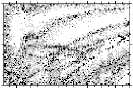
Sample(σexp=0.1)Samplesubscript𝜎exp0.1\text{Sample}\;(\sigma_{\text{exp}}=0.1)Refer to caption1.71.81.92.02.12.22.32.42.5W𝑊W(GeV)-1-0.500.51

cosθc.m.subscript𝜃c.m.\cos\theta_{\text{c.m.}}

Sample(σexp=0.01)Samplesubscript𝜎exp0.01\text{Sample}\;(\sigma_{\text{exp}}=0.01)Refer to caption1.71.81.92.02.12.22.32.42.5W𝑊W(GeV)
Figure 6: Two random samples of the individual events that give rise to the left plots shown in Fig. 5. The gray, black, and white dots correspond with imaginary moduli and/or phases, incorrect phases, and correct phases.

Though having the smaller contribution to the insolvability, incorrect solutions are spurious and should therefore be eliminated, if possible. Incorrect solutions arise from simply marking the solution with the highest ci value as the correct solution. Such a procedure, however, does not stand on statistically solid grounds. A more conservative approach would consist of imposing a tolerance level on the ci values. This would mean that the solution with the highest ci value is only accepted as the correct solution if its confidence interval is greater than or equals the tolerance level. Imposing a tolerance level would not come without a cost, however. The downside of this ‘filtering’ procedure would be a substantial increase in the overall insolvability. Indeed, all of the correct solutions that do not pass the tolerance level would also be rejected and therefore lead to an increase in the insolvability. Nevertheless, the question remains whether such a tolerance requirement can really suppress the fraction of incorrect solutions entirely?

Table 7: The mean confidence intervals ci¯¯ci\overline{\textsc{ci}} for 1000 correct and 1000 incorrect solutions at random kinematical points (W<2500𝑊2500W<2500 MeV and cosθc.m.[1,1]subscript𝜃c.m.11\cos\theta_{\text{c.m.}}\in[-1,1]).
𝝈expsubscript𝝈exp\bm{\sigma_{\text{\bf exp}}} CI¯¯CI\overline{\text{\scriptsize\bf CI}} (%)\bm{(\%)}
Correct Incorrect
0.10.10.1\phantom{00} 93.08.3+4.4subscriptsuperscript93.04.48.393.0^{+4.4}_{-8.3} 91.811.0+5.4subscriptsuperscript91.85.411.091.8^{+5.4}_{-11.0}
0.010.010.01\phantom{0} 91.59.1+5.3subscriptsuperscript91.55.39.191.5^{+5.3}_{-9.1} 88.118.2+7.9subscriptsuperscript88.17.918.288.1^{+7.9}_{-18.2}
0.0010.0010.001 91.78.5+5.0subscriptsuperscript91.75.08.591.7^{+5.0}_{-8.5} 84.922.6+10.0subscriptsuperscript84.910.022.684.9^{+10.0}_{-22.6}

In Table 7, the mean confidence intervals are listed for both 1000 correct and 1000 incorrect solutions at random kinematical points. While the “correct” ci¯¯ci\overline{\textsc{ci}} values are higher than the “incorrect” ones, for each σexpsubscript𝜎exp\sigma_{\text{exp}} value listed, the difference between both is not at all substantial. Moreover, it is seen that a fair fraction of the incorrect solutions have a confidence interval of at least 95%percent9595\%. As there is a significant overlap between the “correct” and “incorrect” ci¯¯ci\overline{\textsc{ci}} values, the entire elimination of the incorrect solutions would require a confidence level so high that nearly all of the correct solutions would get rejected as well, thereby resulting in a practically 100%percent100100\% insolvability. Even lowering the confidence level so as to remove the bulk of the incorrect solutions, would equally wipe out the majority of the correct solutions and hence substantially increase the insolvability.

So, the spurious incorrect solutions can never really be identified, at least not at achievable experimental resolutions. It was shown in the above analysis that even when the confidence interval of a solution is significantly high, it is simply not possible to state whether the solution in question is a correct or an incorrect one. This is in stark contrast with the observation that for a considerable experimental resolution the fraction of incorrect solutions is nearly negligible.

V Conclusions

In this paper, the issue of extracting complete information about reaction amplitudes from pseudoscalar-meson photoproduction data is addressed. The merits of employing the transversity basis (for finite experimental resolution) have been highlighted. Indeed, linear equations connect the moduli of the amplitudes to single-polarization observables. Nonlinear equations connect the relative phases of the amplitudes to double-polarization observables, which are less readily available.

The observables of pseudoscalar-meson photoproduction have been expanded in the transversity basis. An inconsistency with the existing literature is discovered. An independent test of the derived expressions is presented. By rotating the obtained transversity expressions to both the helicity and the CGLN basis, expressions from literature are retrieved. Therefore, convincing evidence has been provided that the derived transversity expansion for the observables is correct.

The extraction of the moduli risubscript𝑟𝑖r_{i} of the normalized transversity amplitudes is a rather straightforward procedure. The authors have performed this analysis for the γpK+Λ𝛾𝑝superscript𝐾Λ\gamma p\to K^{+}\Lambda reaction with sets of {Σ,T,P}Σ𝑇𝑃\{\Sigma,T,P\} data from the GRAAL collaboration. These data cover the range 1.65W1.91less-than-or-similar-to1.65𝑊less-than-or-similar-to1.911.65\lesssim W\lesssim 1.91 GeV. For the moduli, imaginary solutions can be obtained at some isolated kinematics due to finite experimental resolution. In the performed analysis of the GRAAL data, less than 6.5%percent6.56.5\% of the extracted r^isubscript^𝑟𝑖\widehat{r}_{i} are complex. Upon improving the experimental resolution, the fraction of complex r^isubscript^𝑟𝑖\widehat{r}_{i} can be reduced. It is found that the (W,cosθc.m.)𝑊subscript𝜃c.m.(W,\cos\theta_{\text{c.m.}}) dependence of the extracted r^isubscript^𝑟𝑖\widehat{r}_{i} can be nicely reproduced by the RPR-2011 model.

The formalism of Wen-Tai Chiang and Tabakin for solving complete sets has been extended so as to provide consistent estimates for the independent relative phases for data with finite error bars. As a check of this formalism, it was applied to Monte Carlo simulations of the complete set {Cx,Ox,E,F}subscript𝐶𝑥subscript𝑂𝑥𝐸𝐹\{C_{x},O_{x},E,F\} for the reaction γpK+Λ𝛾𝑝superscript𝐾Λ\gamma p\to K^{+}\Lambda. The simulations are generated with the RPR-2011 model.

Estimating the independent phases is far more challenging than determining the moduli. In order to quantify the phase-related issues, the insolvability of the transversity amplitudes has been introduced. The insolvability is a measure for the fraction of complete measurements which does not result in a successful determination of the transversity amplitudes. The insolvability receives contributions from both imaginary and incorrect solutions. It was observed that the fraction of imaginary solutions is much larger for the phases than for the moduli. However, the amount of imaginary solutions can be reduced by increasing the experimental resolution. The ‘incorrect’ component of the insolvability is much more troublesome. It originates from a discrete phase ambiguity that cannot be resolved for finite uncertainties of the asymmetries. Although this component is not the dominant one and decreases for increasing experimental resolution, it was found that at achievable experimental conditions it is impossible to discriminate between correct and incorrect solutions for the phases with statistical significance.

It remains to be investigated whether the measurement of an additional double asymmetry, or multiple ones, could help in resolving the phase ambiguities for realistic experimental resolutions.

Acknowledgements.
This work is supported by the Research Council of Ghent University and the Flemish Research Foundation (FWO Vlaanderen). *

Appendix A Other representations of the asymmetries

A.1 Helicity representation

Table 8: The expressions for the single and double asymmetries in the normalized helicity basis.
Helicity representation
ΣΣ\Sigma Re(h1h4h2h3)Resubscript1superscriptsubscript4subscript2superscriptsubscript3-\text{Re}(h_{1}h_{4}^{*}-h_{2}h_{3}^{*})\phantom{-}
T𝑇T Im(h1h2+h3h4)Imsubscript1superscriptsubscript2subscript3superscriptsubscript4-\text{Im}(h_{1}h_{2}^{*}+h_{3}h_{4}^{*})\phantom{-}
P𝑃P Im(h1h3+h2h4)Imsubscript1superscriptsubscript3subscript2superscriptsubscript4-\text{Im}(h_{1}h_{3}^{*}+h_{2}h_{4}^{*})\phantom{-}
Cxsubscript𝐶superscript𝑥C_{x^{\prime}} Re(h1h3+h2h4)Resubscript1superscriptsubscript3subscript2superscriptsubscript4-\text{Re}(h_{1}h_{3}^{*}+h_{2}h_{4}^{*})\phantom{-}
Czsubscript𝐶superscript𝑧C_{z^{\prime}} 12(|h1|2+|h2|2|h3|2|h4|2)12superscriptsubscript12superscriptsubscript22superscriptsubscript32superscriptsubscript42-\tfrac{1}{2}\left(|h_{1}|^{2}+|h_{2}|^{2}-|h_{3}|^{2}-|h_{4}|^{2}\right)
Oxsubscript𝑂superscript𝑥O_{x^{\prime}} +Im(h1h2h3h4)Imsubscript1superscriptsubscript2subscript3superscriptsubscript4+\text{Im}(h_{1}h_{2}^{*}-h_{3}h_{4}^{*})\phantom{-}
Ozsubscript𝑂superscript𝑧O_{z^{\prime}} Im(h1h4h2h3)Imsubscript1superscriptsubscript4subscript2superscriptsubscript3-\text{Im}(h_{1}h_{4}^{*}-h_{2}h_{3}^{*})\phantom{-}
E𝐸E 12(|h1|2|h2|2+|h3|2|h4|2)12superscriptsubscript12superscriptsubscript22superscriptsubscript32superscriptsubscript42-\tfrac{1}{2}\left(|h_{1}|^{2}-|h_{2}|^{2}+|h_{3}|^{2}-|h_{4}|^{2}\right)
F𝐹F Re(h1h2+h3h4)Resubscript1superscriptsubscript2subscript3superscriptsubscript4-\text{Re}(h_{1}h_{2}^{*}+h_{3}h_{4}^{*})\phantom{-}
G𝐺G +Im(h1h4+h2h3)Imsubscript1superscriptsubscript4subscript2superscriptsubscript3+\text{Im}(h_{1}h_{4}^{*}+h_{2}h_{3}^{*})\phantom{-}
H𝐻H +Im(h1h3h2h4)Imsubscript1superscriptsubscript3subscript2superscriptsubscript4+\text{Im}(h_{1}h_{3}^{*}-h_{2}h_{4}^{*})\phantom{-}
Txsubscript𝑇superscript𝑥T_{x^{\prime}} +Re(h1h4+h2h3)Resubscript1superscriptsubscript4subscript2superscriptsubscript3+\text{Re}(h_{1}h_{4}^{*}+h_{2}h_{3}^{*})\phantom{-}
Tzsubscript𝑇superscript𝑧T_{z^{\prime}} +Re(h1h2h3h4)Resubscript1superscriptsubscript2subscript3superscriptsubscript4+\text{Re}(h_{1}h_{2}^{*}-h_{3}h_{4}^{*})\phantom{-}
Lxsubscript𝐿superscript𝑥L_{x^{\prime}} Re(h1h3h2h4)Resubscript1superscriptsubscript3subscript2superscriptsubscript4-\text{Re}(h_{1}h_{3}^{*}-h_{2}h_{4}^{*})\phantom{-}
Lzsubscript𝐿superscript𝑧L_{z^{\prime}} 12(|h1|2|h2|2|h3|2+|h4|2)12superscriptsubscript12superscriptsubscript22superscriptsubscript32superscriptsubscript42-\tfrac{1}{2}\left(|h_{1}|^{2}-|h_{2}|^{2}-|h_{3}|^{2}+|h_{4}|^{2}\right)

The helicity amplitudes H1,H2,H3,subscript𝐻1subscript𝐻2subscript𝐻3H_{1},H_{2},H_{3}, and H4subscript𝐻4H_{4} are defined as

H1subscript𝐻1\displaystyle H_{1} =+|J+|TR,\displaystyle={}_{R}\langle+|J_{+}|-\rangle_{T},
H2subscript𝐻2\displaystyle H_{2} =+|J+|+TR,\displaystyle={}_{R}\langle+|J_{+}|+\rangle_{T},
H3subscript𝐻3\displaystyle H_{3} =|J+|TR,\displaystyle={}_{R}\langle-|J_{+}|-\rangle_{T},
H4subscript𝐻4\displaystyle H_{4} =|J+|+TR.\displaystyle={}_{R}\langle-|J_{+}|+\rangle_{T}. (42)

Here, |±Tsubscriptketplus-or-minus𝑇|\pm\rangle_{T} and |±Rsubscriptketplus-or-minus𝑅|\pm\rangle_{R} represent the target and recoil helicity eigenstates, respectively, and J+subscript𝐽J_{+} is defined in Eq. (9). As the target (recoil) momentum pTsubscript𝑝𝑇\vec{p}_{T} (pRsubscript𝑝𝑅\vec{p}_{R}) is directed along the negative z𝑧z–axis (zsuperscript𝑧z^{\prime}–axis), it follows that

|±Tsubscriptketplus-or-minus𝑇\displaystyle|\pm\rangle_{T} =|±z=u±(pT,π,0),absentsubscriptketplus-or-minus𝑧subscript𝑢plus-or-minussubscript𝑝𝑇𝜋0\displaystyle=|\pm\rangle_{-z}=u_{\pm}(p_{T},\pi,0),
|±Rsubscriptketplus-or-minus𝑅\displaystyle|\pm\rangle_{R} =|±z=u±(pR,πθc.m.,π).absentsubscriptketplus-or-minussuperscript𝑧subscript𝑢plus-or-minussubscript𝑝𝑅𝜋subscript𝜃c.m.𝜋\displaystyle=|\pm\rangle_{-z^{\prime}}=u_{\pm}(p_{R},\pi-\theta_{\text{c.m.}},\pi). (43)

From Eqs. (2), (3), (4), and (43) one deduces the following relations

|±Tsubscriptketplus-or-minus𝑇\displaystyle|\pm\rangle_{T} =12(i|±y|y),absentminus-or-plus12𝑖subscriptketplus-or-minus𝑦subscriptketminus-or-plus𝑦\displaystyle=\mp\frac{1}{\sqrt{2}}\Bigl{(}i|\pm\rangle_{y}-|\mp\rangle_{y}\Bigr{)},
|±Rsubscriptketplus-or-minus𝑅\displaystyle|\pm\rangle_{R} =±12(ieiθc.m./2|±ye±iθc.m./2|y),absentplus-or-minus12𝑖superscript𝑒minus-or-plus𝑖subscript𝜃c.m.2subscriptketplus-or-minus𝑦superscript𝑒plus-or-minus𝑖subscript𝜃c.m.2subscriptketminus-or-plus𝑦\displaystyle=\pm\frac{1}{\sqrt{2}}\Bigl{(}ie^{\mp i\theta_{\text{c.m.}}/2}|\pm\rangle_{y}-e^{\pm i\theta_{\text{c.m.}}/2}|\mp\rangle_{y}\Bigr{)}, (44)

and in combination with the definition of Jsubscript𝐽J_{-} in Eq. (9), one can readily show that the following properties hold

H1subscript𝐻1\displaystyle H_{1} =+|J+|TR=+|J|+TR,\displaystyle={}_{R}\langle+|J_{+}|-\rangle_{T}=+{}_{R}\langle-|J_{-}|+\rangle_{T},
H2subscript𝐻2\displaystyle H_{2} =+|J+|+TR=|J|TR,\displaystyle={}_{R}\langle+|J_{+}|+\rangle_{T}=-{}_{R}\langle-|J_{-}|-\rangle_{T},
H3subscript𝐻3\displaystyle H_{3} =|J+|TR=+|J|+TR,\displaystyle={}_{R}\langle-|J_{+}|-\rangle_{T}=-{}_{R}\langle+|J_{-}|+\rangle_{T},
H4subscript𝐻4\displaystyle H_{4} =|J+|+TR=++|J|TR.\displaystyle={}_{R}\langle-|J_{+}|+\rangle_{T}=+{}_{R}\langle+|J_{-}|-\rangle_{T}. (45)

From Eqs. (10), (9), (42), and (44), one then obtains

Hi=12Uijbj,subscript𝐻𝑖12subscript𝑈𝑖𝑗subscript𝑏𝑗\displaystyle H_{i}=\frac{1}{\sqrt{2}}U_{ij}b_{j}, (46)

with U𝑈U a unitary matrix (UU=UU=1)superscript𝑈𝑈𝑈superscript𝑈1\left(U^{\dagger}U=UU^{\dagger}=1\right)

U=eiθc.m./22(1eiθc.m.1eiθc.m.iieiθc.m.iieiθc.m.iieiθc.m.iieiθc.m.1eiθc.m.1eiθc.m.).𝑈superscript𝑒𝑖subscript𝜃c.m.22matrix1superscript𝑒𝑖subscript𝜃c.m.1superscript𝑒𝑖subscript𝜃c.m.𝑖𝑖superscript𝑒𝑖subscript𝜃c.m.𝑖𝑖superscript𝑒𝑖subscript𝜃c.m.𝑖𝑖superscript𝑒𝑖subscript𝜃c.m.𝑖𝑖superscript𝑒𝑖subscript𝜃c.m.1superscript𝑒𝑖subscript𝜃c.m.1superscript𝑒𝑖subscript𝜃c.m.\displaystyle U=\frac{e^{i\theta_{\text{c.m.}}/2}}{2}\begin{pmatrix}1&-e^{-i\theta_{\text{c.m.}}}&-1&-e^{-i\theta_{\text{c.m.}}}\\ i&ie^{-i\theta_{\text{c.m.}}}&i&-ie^{-i\theta_{\text{c.m.}}}\\ i&ie^{-i\theta_{\text{c.m.}}}&-i&ie^{-i\theta_{\text{c.m.}}}\\ -1&e^{-i\theta_{\text{c.m.}}}&-1&-e^{-i\theta_{\text{c.m.}}}\end{pmatrix}. (47)

The ‘normalized’ helicity amplitudes hisubscript𝑖h_{i}

hi=2Hi|H1|2+|H2|2+|H3|2+|H4|2,subscript𝑖2subscript𝐻𝑖superscriptsubscript𝐻12superscriptsubscript𝐻22superscriptsubscript𝐻32superscriptsubscript𝐻42\displaystyle h_{i}=\frac{\sqrt{2}H_{i}}{\sqrt{|H_{1}|^{2}+|H_{2}|^{2}+|H_{3}|^{2}+|H_{4}|^{2}}}, (48)

can be written in terms of the normalized transversity amplitudes aisubscript𝑎𝑖a_{i} of Eq. (17)

ai=12(U)ijhj=12Ujihj.subscript𝑎𝑖12subscriptsuperscript𝑈𝑖𝑗subscript𝑗12subscriptsuperscript𝑈𝑗𝑖subscript𝑗\displaystyle a_{i}=\frac{1}{\sqrt{2}}(U^{\dagger})_{ij}h_{j}=\frac{1}{\sqrt{2}}U^{*}_{ji}h_{j}. (49)

Hereby, use is made of the unitarity of U𝑈U. From the above relations and the expressions of Table 1, one obtains the helicity representation (Table 8) of the polarization observables. The {Ax,Az}subscript𝐴superscript𝑥subscript𝐴superscript𝑧\{A_{x^{\prime}},A_{z^{\prime}}\} (A{C,O,T,L}𝐴𝐶𝑂𝑇𝐿A\in\{C,O,T,L\}) are related to the {Ax,Az}subscript𝐴𝑥subscript𝐴𝑧\{A_{x},A_{z}\} through

(AxAz)=(cosθc.m.sinθc.m.sinθc.m.cosθc.m.)(AxAz).matrixsubscript𝐴superscript𝑥subscript𝐴superscript𝑧matrixsubscript𝜃c.m.subscript𝜃c.m.subscript𝜃c.m.subscript𝜃c.m.matrixsubscript𝐴𝑥subscript𝐴𝑧\displaystyle\begin{pmatrix}A_{x^{\prime}}\\ A_{z^{\prime}}\end{pmatrix}=\begin{pmatrix}\cos\theta_{\text{c.m.}}&-\sin\theta_{\text{c.m.}}\\ \sin\theta_{\text{c.m.}}&\cos\theta_{\text{c.m.}}\end{pmatrix}\begin{pmatrix}A_{x}\\ A_{z}\end{pmatrix}. (50)

The expressions of Table 8 coincide with those in Ref. Fasano:1992es .

A.2 CGLN representation

The Chew-Goldberger-Low-Nambu (CGLN) amplitudes Fisubscript𝐹𝑖F_{i} are, for example, defined in Eq. (8) of Ref. Sandorfi:2011nv . In what follows a connection is established between the the CGLN and the transversity amplitudes, as this might be useful for future analyses. From the definition of the Dirac spinor (2), the reduced CGLN amplitudes fi=ρ0Fisubscript𝑓𝑖subscript𝜌0subscript𝐹𝑖f_{i}=\sqrt{\rho_{0}}F_{i} can be related to the aisubscript𝑎𝑖a_{i} of Eq. (17). Here, ρ0subscript𝜌0\rho_{0} is the density-of-states factor, defined in Eq. (5) of Ref. Sandorfi:2011nv . The following relation holds

fi=Vijaj,subscript𝑓𝑖subscript𝑉𝑖𝑗subscript𝑎𝑗\displaystyle f_{i}=V_{ij}a_{j}, (51)

with V𝑉V a non-unitary matrix, given by

V=isin2θc.m.(ieiθc.m.ieiθc.m.00isinθc.m.isinθc.m.00eiθc.m.eiθc.m.eiθc.m.eiθc.m.1111).𝑉𝑖superscript2subscript𝜃c.m.matrix𝑖superscript𝑒𝑖subscript𝜃c.m.𝑖superscript𝑒𝑖subscript𝜃c.m.00𝑖subscript𝜃c.m.𝑖subscript𝜃c.m.00superscript𝑒𝑖subscript𝜃c.m.superscript𝑒𝑖subscript𝜃c.m.superscript𝑒𝑖subscript𝜃c.m.superscript𝑒𝑖subscript𝜃c.m.1111\displaystyle V=-\frac{i}{\sin^{2}\theta_{\text{c.m.}}}\begin{pmatrix}ie^{i\theta_{\text{c.m.}}}&ie^{-i\theta_{\text{c.m.}}}&0&0\\ i\sin\theta_{\text{c.m.}}&i\sin\theta_{\text{c.m.}}&0&0\\ -e^{i\theta_{\text{c.m.}}}&e^{-i\theta_{\text{c.m.}}}&e^{i\theta_{\text{c.m.}}}&e^{-i\theta_{\text{c.m.}}}\\ 1&-1&-1&-1\end{pmatrix}. (52)

This means that the CGLN basis is not orthogonal. By substituting ai=(V1)ijfjsubscript𝑎𝑖subscriptsuperscript𝑉1𝑖𝑗subscript𝑓𝑗a_{i}=(V^{-1})_{ij}f_{j} in Table 1, with

V1=i2(1eiθc.m.001eiθc.m.001eiθc.m.isinθc.m.ieiθc.m.sinθc.m.1eiθc.m.isinθc.m.ieiθc.m.sinθc.m.),superscript𝑉1𝑖2matrix1superscript𝑒𝑖subscript𝜃c.m.001superscript𝑒𝑖subscript𝜃c.m.001superscript𝑒𝑖subscript𝜃c.m.𝑖subscript𝜃c.m.𝑖superscript𝑒𝑖subscript𝜃c.m.subscript𝜃c.m.1superscript𝑒𝑖subscript𝜃c.m.𝑖subscript𝜃c.m.𝑖superscript𝑒𝑖subscript𝜃c.m.subscript𝜃c.m.\displaystyle V^{-1}=\frac{i}{2}\begin{pmatrix}-1&e^{-i\theta_{\text{c.m.}}}&0&0\\ 1&-e^{i\theta_{\text{c.m.}}}&0&0\\ -1&e^{-i\theta_{\text{c.m.}}}&-i\sin\theta_{\text{c.m.}}&-ie^{-i\theta_{\text{c.m.}}}\sin\theta_{\text{c.m.}}\\ -1&e^{i\theta_{\text{c.m.}}}&i\sin\theta_{\text{c.m.}}&ie^{i\theta_{\text{c.m.}}}\sin\theta_{\text{c.m.}}\end{pmatrix}, (53)

one retrieves the CGLN expansion of the asymmetries as is listed in Eqs. (58b–p) of Ref. Sandorfi:2011nv .

As Vsin2θc.m.proportional-to𝑉superscript2subscript𝜃c.m.V\propto\sin^{-2}\theta_{\text{c.m.}}, it is divergent at cosθc.m.=±1subscript𝜃c.m.plus-or-minus1\cos\theta_{\text{c.m.}}=\pm 1. In these two cases, the CGLN amplitudes cannot be expressed in terms of the transversity ones. Conversely, for cosθc.m.=±1subscript𝜃c.m.plus-or-minus1\cos\theta_{\text{c.m.}}=\pm 1 the aisubscript𝑎𝑖a_{i} can be expanded in the fisubscript𝑓𝑖f_{i} basis, though. By substituting cosθc.m.=±1subscript𝜃c.m.plus-or-minus1\cos\theta_{\text{c.m.}}=\pm 1 in ai=(V1)ijfjsubscript𝑎𝑖subscriptsuperscript𝑉1𝑖𝑗subscript𝑓𝑗a_{i}=(V^{-1})_{ij}f_{j}, it is found that

a1=a2=a3=a4=i2(f1f2).subscript𝑎1subscript𝑎2subscript𝑎3subscript𝑎4𝑖2minus-or-plussubscript𝑓1subscript𝑓2\displaystyle a_{1}=-a_{2}=a_{3}=a_{4}=-\frac{i}{2}(f_{1}\mp f_{2}). (54)

The normalization condition (18) then leads to |ai|=12subscript𝑎𝑖12|a_{i}|=\frac{1}{2} for cosθc.m.=±1subscript𝜃c.m.plus-or-minus1\cos\theta_{\text{c.m.}}=\pm 1. As a consequence, by invoking Table 1, all the single and double asymmetries can be quantified at these two extreme angles. At cosθc.m.=±1subscript𝜃c.m.plus-or-minus1\cos\theta_{\text{c.m.}}=\pm 1 one has that Cz=E=1subscript𝐶𝑧𝐸1C_{z}=E=1 and Lz=1subscript𝐿𝑧1L_{z}=-1, while all other asymmetries vanish. This result holds for any possible value of W𝑊W. It is quite remarkable that this interesting general result can be derived by altering the representation of the amplitudes.

References