Reversible limit of processes of heat transfer

Abstract

We study a process of heat transfer between a body of heat capacity $C(T)$ and a sequence of $N$ heat reservoirs, with temperatures equally spaced between an initial temperature $T_{0}$ and a final temperature $T_{N}$. The body and the heat reservoirs are isolated from the rest of the universe, and the body is brought in thermal contact successively with reservoirs of increasing temperature. We determine the change of entropy of the composite thermodynamic system in the total process in which the temperature of the body changes from $T_{0}$ to $T_{N}$. We find that for large values of $N$ the total change of entropy of the composite process is proportional to $(T_{N}-T_{0})/N$, but eventually a non-monotonic behavior is found at small values of $N$.

I Introduction

One of the original formulations of the second law of thermodynamics, due to Clausius, states that “no process is possible whose only result is the transfer of heat from a body of lower temperature to a body of higher temperature”. As discussed by Fermi in his book fermi , since as this statement was made the concept of temperature was empirical, to find out which of two bodies has the higher temperature one had to put them in thermal contact and find out in which sense the heat flows, it will flow spontaneously from the body of higher temperature to the other. So, Clausius’s statement could be rephrased into “If heat flows spontaneously from body A to body B, no process is possible whose only result is the transfer of heat from body B to body A”. To be more precise, let us isolate the two bodies from the rest of the universe, to assure that they will not exchange heat or other forms of energy with the environment, this is implicit in the term ‘only result’. We may notice in this statement that already the idea of irreversibility is present: if heat flows spontaneously from A to B, it will not flow spontaneously from B to A. In other words, the process of transfer of heat between two bodies which are isolated from the environment is irreversible.

The second law off thermodynamics says that not all processes which conserve energy, as required by the first law, occur in nature. In many cases (if not all), if a given process in an isolated system occurs, the inverse process does not. This idea was further formalized by the introduction of the concept of entropy, so that processes in isolated systems which lead to a decrease of the entropy are not allowed. In particular, in the process of heat transfer mentioned above, the entropy of the composite isolated system increases if the heat flows from the body of higher temperature to the one of lower temperature, but would decrease in the inverse process, so that only the further is allowed. It is interesting to recall that in his paper of 1885, Clausius summarized the two first laws of thermodynamics in just two sentences: “The energy of the universe is constant. The entropy of the universe tends to a maximum” clausius . We may notice that the universe is the only composite thermodynamic system which is isolated by definition.

The entropy in equilibrium thermodynamics is a state function, so that it is defined for equilibrium states of the system. When two bodies of different temperatures are brought into thermal contact, the composite system in general will go through a sequence of non-equilibrium states, but if we wait long enough, it will finally reach a new equilibrium state, where both bodies of the composite have the same temperature, and in this state the entropy is larger than it was in the initial state. If we now imagine a process which happens at a very slow rate in time when compared to the relaxation time of the system callen , we may reach a situation close to the one in which all intermediate states of the system are equilibrium states. In this limit the process is called quasi-static, and therefore the whole process may be represented as a path in the space of variables which define the equilibrium states of the system. In the particular case in which the entropy of the final state of the quasi-static process is equal to the entropy of the initial state, and therefore to the entropies of all intermediate states, this process will be reversible.

The process we will study in some detail here is the transfer of heat in isolated systems composed by a heat reservoir (constant temperature) and a body whose heat capacity is described by a function $C(T)$. The initial temperature of the body is $T_{0}$ and its final temperature is $T_{N}$. The change of the temperature of the body is accomplished by putting it in thermal contact with a sequence of $N$ heat reservoirs whose temperatures are equally spaced between $T_{0}$ and $T_{N}$. For a finite number of reservoirs, each of the sub-processes consists of heat transfer between two bodies at different temperatures and is therefore irreversible, leading to an increase of the entropy of the composite isolated system. In the limit $N\to\infty$, however, each sub-process will contribute with a negligible increase of entropy and, what may not be obvious initially, the total variation of entropy vanishes as well, so that this is a concrete example of a limit which leads to a reversible, quasi-static process of heat transfer.

This problem, of considerable pedagogical interest, has been studied before in the literature. For a constant heat capacity, such as is found for ideal gases, Calkin and Kiang ck83 have shown for a cyclic process ($T_{0}\to T_{N}\to T_{0}$), that the total change of entropy vanishes as $1/N$ in the limit $N\to\infty$ because, although the number of sub-processes increases, the increase of entropy in each of them is proportional to $1/N^{2}$ in this limit. A similar situation is proposed in the exercise 4.4-6 in Callen’s book callen . The same process was studied also by Thomsen and Bers tb96 , again for the case of constant heat capacity and discussing in detail that it is always possible, given any positive value $\epsilon$, to choose a value of $N$ for which the increase of entropy is smaller than $\epsilon$. This argument is then repeated for the inverse process, thus characterizing the process in the limit $N\to\infty$ as reversible.

Here we generalize the problem in two ways: the heat capacity of the system is no longer constant and we develop the increase of entropy as a series in $1/N$, so that we find the corrections to the leading term. We also show that some symmetries in the result which are valid in the asymptotic limit close to reversibility are not longer present for finite values of $N$. In particular, we show that, although in the large $N$ limit the increase of entropy decreases monotonically with $N$, this may not happen at lower numbers of heat reservoirs. Also, the increase of entropy for the direct process ($T_{0}\to T_{N}$) may be different of the same quantity for the inverse process ($T_{N}\to T_{0}$). The determination of the change of entropy is given in section II and applications to particular cases and final comments may be found in section III.

II Determination of the change of entropy

Let us define the problem in more detail. Our composite system consists of the body, whose heat capacity is $C(T)$ and which will undergo a temperature change $\Delta T=T_{N}-T_{0}$, and a set of $N$ heat reservoirs, at equally spaced temperatures, so that the temperature of the reservoir $j$ ($j=1,2,3,\ldots,N$) is equal to $T_{j}=T_{0}+j\,\Delta T/N$. The body is brought into thermal contact with the heat reservoirs in order of increasing values of $j$ until its temperature equals the one of the reservoir and therefore is increased bi $\Delta T/N$. In the first sub-process, for example, the body starts with temperature $T_{0}$ and ends with temperature $T_{0}+\Delta T/N$. After the $N$’th process, the body will reach the final temperature $T_{N}$. This sequence of heat transfer processes is illustrated in figure 1. Actually, one could argue that the time required to reach equilibrium for each sub-process of heat transfer would be infinite, and for this reason, Thomsen and Bers, in their discussion of a similar process tb96 , have chosen the temperature of the $j$’th reservoir to be $T_{0}+(j+1)\Delta T/N$, thus assuring that the equilibration time of the system with each reservoir is finite. Here, for simplicity, we will not use this improved version of the process.

Figure 1: Illustration of the $j$’th process of heat transfer, where the system $s$ is in thermal contact with the heat reservoir at temperature $T_{j}$, so that its temperature is changed from $T_{j-1}$ to $T_{j}$. The pair system-reservoir at $T_{j}$ is isolated, as are all the other reservoirs.

If a the body, at temperature $T$, receives a quantity of heat $dQ_{b}$, its temperature will change by $dT=dQ_{b}/C(T)$. The change of entropy of the body in the whole sequence of heat transfer processes is:

$$\Delta S_{b}=\int_{T_{0}}^{T_{N}}\frac{dQ_{b}}{T}=\\ \int_{T_{0}}^{T_{N}}\frac{C(T)}{T}\,dT.$$

The change of entropy of all reservoirs in the sequence of processes will be:

$$\Delta S_{r}(N) = \sum_{j=1}^{N}\Delta S_{r}(N,j)=\sum_{j=1}^{N}\frac{1}{T_{j}}\int_{T_{j-1}}^{T_{j}}dQ_{r}=$$ (1)

$$-\sum_{j=1}^{N}\frac{1}{T_{j}}\int_{T_{j-1}}^{T_{j}}C(T)\,dT,$$

where in the last passage, we recall that in each sub-process, the body and the reservoir are isolated, so that the heat received by the reservoir is given by $dQ_{r}=-dQ_{b}=-C(T)\,dT$. We thus may write the total change of entropy as:

$$\Delta S(N) = \Delta S_{b}(N)+\Delta S_{r}(N)=$$ (2)

$$\int_{T_{0}}^{T_{N}}\frac{C(T)}{T}\,dT-\sum_{j=1}^{N}\frac{1}{T_{j}}\int_{T_{j-1}}^{T_{j}}C(T)\,dT.$$

If it is possible to perform both integrations, this expression above becomes:

$$\Delta S(N)=S_{b}(T_{N})-S_{b}(T_{0})-\sum_{j=1}^{N}\frac{1}{T_{j}}[U(T_{j})-U(T_{j-1})],$$ (3)

where $S_{b}(T)=\int C(T)/T\,dT$ and $U(T)=\int C(T)\,dT$. It is convenient to rewrite the expression for the change of entropy as:

$$\Delta S(N)=\sum_{j=1}^{N}\int_{T_{j-1}}^{T_{j}}\kappa_{j}(T,N)\phi(T)\,dT,$$ (4)

where $\kappa_{j}(T,N)=1-T/T_{j}$ and $\phi(T)=C(T)/T$. It is now easy to see that, since stability implies that $\phi(T)\geq 0$, we must have $\Delta S\geq 0$, as required by the second law of thermodynamics. Let us show this in some detail. Suppose that $T_{N}>T_{0}$, so that the temperature of the body increases in the process. It is then clear that $\kappa_{j}(T,N)\geq 0$ and as a consequence the entropy of the composite system increases. The same happens in the inverse process, where the temperature of the body decreases from $T_{N}$ to $T_{0}$. In this case the change if entropy is:

$$\Delta S^{\prime}(N)=-\sum_{j=1}^{N}\int_{T_{j-1}}^{T_{j}}\kappa_{j-1}(T,N)\phi(T)\,dT,$$ (5)

and since now $\kappa_{j-1}(T,N)\leq 0$ in the range of integration, again the entropy increases. It may be worth noticing that the difference of the entropy increases between the processes with raising and lowering of the temperature of the body $\delta S(N)=\Delta S^{\prime}(N)-\Delta S(N)$ is:

$$\delta S(N)=\sum_{j=1}^{N}\int_{T_{j-1}}^{T_{j}}\left[\left(\frac{1}{T_{j-1}}+\frac{1}{T_{j}}\right)T-2\right]\phi(T)\,dT,$$ (6)

and the sign of this expression is not defined in general.

Another general property of the entropy increase is its dependence of the number of reservoirs $N$. As we will see below, it vanishes in the limit $N\to\infty$ of a quasi-static process. The question we will address is if the change of the entropy decreases monotonically with $N$. For convenience, we will define the function:

$$\kappa(T,N)=\sum_{j=1}^{N}\Theta(T-T_{j-1})\Theta(T_{j}-T)\,\kappa_{j}(T,N),$$ (7)

where $\Theta(T)$ is the step function. The function $\kappa(T,N)$ is defined in the whole temperature range $[T_{0},T_{N}]$ and has a sawtooth pattern, with $N$ maxima of decreasing values. The expression for the entropy increase Eq. (4) may then be cast into the following form:

$$\Delta S(N)=\int_{T_{0}}^{T_{N}}\kappa(T,N)\phi(T)\,dT.$$ (8)

The difference of entropy increases for two values of $N$, ($N_{2}>N_{1}$) is:

$$\Delta S(N_{1})-\Delta S(N_{2})=\int_{T_{0}}^{T_{N}}[\kappa(T,N_{1})-\kappa(T,N_{2})]\phi(T)\,dT.$$ (9)

It is straightforward to see that if $N_{2}$ is a multiple of $N_{1}$ the difference of $\kappa$ functions is non-negative, and therefore $\Delta S(N_{1})-\Delta S(nN_{1})\geq 0$ for any integer $n$. For example, we have $\Delta S(1)>\Delta S(2)$. This, however, is no longer true in general if the ratio $N_{2}/N_{1}$ is not an integer. As an example, in figure 2 we show the difference of $\kappa$ functions for $N_{1}=5$ and $N_{2}=6$, and we notice that this difference assumes negative values in part of the temperature domain. We thus reach the conclusion that, depending on the function $\phi(T)$, the entropy increase for $N_{2}$ heat reservoirs may be larger than the one for $N_{1}$ reservoirs, if $1<N_{2}/N_{1}<2$.

Figure 2: The function $\kappa(T,5)-\kappa(T,6)$ for initial temperature $T_{0}=10$ and final temperature $T_{N}=20$.

We now proceed obtaining the general asymptotic behavior of $\Delta S(N)$ for $N\gg 1$. Expanding the last integral in the expression for the increase of entropy, Eq. (2), which corresponds to the amount of heat $Q_{j}$ exchanged by the body with reservoir $j$, in a Taylor series around the temperature $T_{j}$, we get:

$$Q_{j}=-\sum_{i=1}^{\infty}\frac{(-1)^{i}}{i\!}\left(\frac{\Delta T}{N}\right)^{i}C^{(i-1)}(T_{j}),$$ (10)

where a superscript between parenthesis means a derivative of the corresponding function of the order of the superscript. We may now write the total change of entropy as:

$$\Delta S(N) = \int_{T_{0}}^{T_{N}}\frac{C(T)}{T}\,dT+$$ (11)

$$\sum_{i=1}^{\infty}\frac{(-1)^{i}}{i\!}\left(\frac{\Delta T}{N}\right)^{i}\sum_{j=1}^{N}\frac{C^{(i-1)}(T_{j})}{T_{j}}.$$

We now proceed transforming the sum over the reservoirs into an integral, using Euler-MacLaurin’s expansion knopp :

$$\sum_{i=m}^{n}f(i) = \int_{m}^{n}f(x)\,dx+\frac{1}{2}[f(n)+f(m)]+$$ (12)

$$\sum_{k=1}^{k_{max}}\frac{B_{2k}}{(2k)!}\left[f^{(2k-1)}(n)-f^{(2k-1)}(m)\right]+$$

$$R_{k_{max}},$$

where $B_{2k}$ are the Bernoulli numbers ($B_{2}=1/6$, $B_{4}=-1/30$, $B_{6}=1/42$, $B_{8}=-1/30$, $\ldots$. See bn for a list of the numbers). The series in the right hand side is divergent in many cases, since the Bernoulli numbers increase very fast for larger values of $k$. There are procedures to evaluate the rest $R_{k_{max}}$ knopp and we will discuss this issue in the appendix. The sum we will convert into an integral is:

$$G_{i}=\sum_{j=1}^{N}\frac{C^{(i-1)}(T_{j})}{T_{j}}=\sum_{j=0}^{N}\frac{C^{(i-1)}(T_{j})}{T_{j}}-\frac{C^{(i-1)}(T_{0})}{T_{0}},$$ (13)

and applying the expansion (12) we find:

$$G_{i} = \frac{N}{\Delta T}\int_{T_{0}}^{T_{N}}\frac{C(T)^{(i-1)}}{T}\,dT+$$ (14)

$$\frac{1}{2}\left[\frac{C^{(i-1)}(T_{N})}{T_{N}}-\frac{C^{(i-1)}(T_{0})}{T_{0}}\right]+$$

$$\sum_{k=1}^{k_{max}}\frac{B_{2k}}{(2k)!}\left(\frac{\Delta T}{N}\right)^{2k-1}\times$$

$$\left[\left(\frac{C^{(i-1)}(T_{N})}{T_{N}}\right)^{(2k-1)}-\right.$$

$$\left.\left(\frac{C^{(i-1)}(T_{0})}{T_{0}}\right)^{(2k-1)}\right]+R_{k_{max}}.$$

Now we may substitute this last expression into Eq. (11) and collect the terms in the change of entropy of the body in the sequence of processes in powers of $1/N$. We notice, as expected, than the term of order $0$ cancels, so that, in the limit $N\to\infty$ the whole process becomes reversible. In the appendix, we proceed calculating all coefficients $\sigma_{i}$ of the expansion

$$\Delta S(N)=\sum_{i=1}^{i_{max}}\sigma_{i}\left(\frac{1}{N}\right)^{i},$$ (15)

but here we we will limit ourselves to the leading term, which is:

$$\sigma_{1}=\frac{T_{N}-T_{0}}{2}\left[\int_{T_{0}}^{T_{N}}\frac{C^{(1)}(T)}{T}\,dT-\left(\frac{C(T_{N})}{T_{N}}+\frac{C(T_{0})}{T_{0}}\right)\right].$$ (16)

Integrating by parts, we finally obtain the leading term of the expansion:

$$\Delta S(N)\approx\frac{T_{N}-T_{0}}{2N}\int_{T_{0}}^{T_{N}}\frac{C(T)}{T^{2}}\,dT,$$ (17)

valid in the limit $N\gg 1$.

Since $C(T)\geq 0$, we notice that the leading term vanishes only in the trivial case where $C(T)=0$ in the whole range of temperatures and there is no heat transfer, so that the asymptotic behavior as $1/N$ in the increase of entropy, as was found in the particular case of an ideal gas ck83 , is universal. We also remark that in the asymptotic regime the entropy increase is invariant if the temperatures are interchanged and also monotonically decreasing with $N$, properties which are not true in general for small values of the number of reservoirs.

III Discussions and conclusion

We will now apply the results of the preceding section to some particular cases of physical interest. We start with the ideal gas, which has a constant heat capacity $C(T)=C_{0}$. Applying Eq. (2) to this particular case, the increase of the entropy will be:

$$\frac{\Delta S(N)}{C_{0}}=\ln f-\frac{f-1}{N}\sum_{j=1}^{N}\frac{1}{1+\frac{j}{N}(f-1)},$$ (18)

where $f=T_{N}/T_{0}$. The leading term in this case is:

$$\frac{\Delta S(N)}{C_{0}}\approx\frac{1}{2N}\left(\sqrt{f}-\sqrt{1/f}\right)^{2}.$$ (19)

In figure 3 we show some curves of the entropy increase as a function of $1/N$, for different values of the ratio of temperatures $f$, as well as the dashed straight lines which represent the asymptotic behavior. Notice that, as expected, the same asymptotic behavior is found for $f=2$ and $f=1/2$. If we consider two processes, one with ratio $f_{1}>1$ and the other with $f_{2}=1/f_{1}<1$, that is, related by interchange of the temperatures, both will have the same asymptotic behavior, as may be seen in the particular cases depicted in the figure. Also, the increase of entropy in the second process, where the body is cooled, is always larger than the one in the first process. Another way to state the same property is that, as can be seen in the curves, the increase of entropy is a concave function of $1/N$ for processes where the body is heated and it is a convex function when the temperature of the body decreases. In the asymptotic regime these properties may be obtained the next term of the Euler-MacLaurin expansion, as will be discussed in the appendix. Also, the increase of entropy for this particular case is a monotonically decreasing function of $N$.

Figure 3: Increase of entropy for a system with constant heat capacity $C_{0}$ (ideal gas) as a function of the inverse number of reservoirs $1/N$. The four curves, in the upward order, correspond to ratios of temperatures $f=T_{N}/T_{0}=2,\;1/2,\;5$ and $1/5$. The dashed straight lines are the asymptotic behavior for small $1/N$.

In most cases the variation of entropy decreases monotonically with $N$, a property which seems also intuitive, since by decreasing the temperature steps in a certain sense the composite process gets closer to a reversible process. For the ideal gas this is always the case. We have seen above, however, that this may not be generally true. If we look at the Eq. (9) for the difference of entropy increases for different values of $N$, a non-monotonic result is possible if the function $\phi(T)$ has one or more peaks at the temperatures where $\kappa(T,N_{1})-\kappa(T,N_{2})$ is negative. One system which could possibly show a non-monotonic behavior is a two-state system callen , since its heat capacity displays a peak, sometimes called “Schottky hump”. However, we found that this is not the case, the reason is that the peak is too wide to produce a non-monotonic behavior.

We turn our attention to a situation where the width of the peak in the heat capacity may be changed by adjusting a parameter. The simple expression we will use for the heat capacity is:

$$C(T)=C[\tau(2-\tau)]^{m},$$ (20)

where $\tau=T/T_{c}$, so that $T_{c}$ is the temperature where the maximum of the heat capacity is located, and $C$ is a constant with the dimension of entropy. Although this heat capacity does not correspond to a particular physical system, it is convenient for analytic calculations and consistent with the third law of thermodynamics. Of course, at least for odd values of the parameter $m$, it is valid only if $\tau$ is in the range $[0,2]$, so we will restrict ourselves to this range of temperatures. As the parameter $m$ grows, the peak in $C(T)$ narrows, and our main interest in this system is that, for sufficiently large values of $m$, non-monotonic behavior is found in $\Delta S(N)$.

In figure 4 we show, in the same graph, the function $\kappa(\tau,2)-\kappa(\tau,3)$ and the function $\phi(\tau)=C(\tau)/(C\tau)$, given by Eq. (20) with $m=16$. As is apparent in the graph, with the choices of initial ($\tau_{0}=0.286$) and final ($\tau_{N}=2.0$) temperatures we made, the maximum of the peak in $C(T)$ is close to the center of the negative peak in $\kappa(\tau,2)-\kappa(\tau,3)$, so that the difference $\Delta S(2)-\Delta S(3)$ is minimized, since this difference is given by Eq. (9). In table 1 we list the results for $[\Delta S(3)-\Delta S(2)]/C$ for different values of $m$, with the choices above for $\tau_{0}$ and $\tau_{N}$, and it is clear that a non-monotonic behavior is found for $m\geq 16$. Finally, we found some evidence that a local maximum in the entropy could also be found at $N=4$, but if this actually happens for this particular form of heat capacity, it will be at rather large values of $m$, which lead to numerical problems. We remark that, in order to reduce numerical errors, in all examples we discuss the integrations involved in the calculation of the entropy increase Eq. (2) are performed analytically, as is done in Eq. (3).

Figure 4: $\kappa(\tau,2)-\kappa(\tau,3)$ (dashed line) and the function $\phi(\tau)=C(\tau)/(C\tau)=[\tau(2-\tau)]^{16}/\tau$. The initial temperature is $\tau_{0}=0.286$ and the final temperature is $\tau_{N}=2.0$

$m$	$[\Delta S(3)-\Delta S(2)]/C$
$14$	$-3.158309\times 10^{-3}$
$15$	$-3.427008\times 10^{-4}$
$16$	$2.185200\times 10^{-3}$
$17$	$4.463576\times 10^{-3}$

Table 1: $[\Delta S(3)-\Delta S(2)]/C$ for different values of the parameter $m$ for a system with heat capacity given by Eq. (20). The temperature range of the process is $\tau_{0}=0.286$, $\tau_{N}=2.0$.

As discussed before, we expect, qualitatively, the non-monotonic behavior to be enhanced if the peak in the heat capacity is more pronounced. This leads us, in this final example, to a system which undergoes a continuous phase transition, since in this case a singularity at the critical temperature $T_{c}$ is found in the heat capacity, of the form $C(T)\approx|1-T/T_{c}|^{-\alpha}$, described by the critical exponent $\alpha$ yeomans . To the singular behavior of the heat capacity, usually regular contributions should be added, so that we will use the simple expression:

$$C(T)=C\tau|1-\tau|^{-\alpha},$$ (21)

where we define the reduced dimensionless temperature $\tau=T/T_{c}$ and which is compatible with the third law of thermodynamics. It should be mentioned that since the exchange of heat when the temperature of the body crosses the critical temperature has to be finite, we should restrict the critical exponent $\alpha$ to values smaller than $1$. It is easy to perform the necessary integrations in this case, so that the entropy increase will be given by Eq. (3) with:

$$\frac{S_{b}(\tau)}{C}=\left\{\begin{array}[]{ll}-\frac{(1-\tau)^{1-\alpha}}{1-\alpha},&\mbox{$\tau<1$,}\\ &\\ \frac{(\tau-1)^{1-\alpha}}{1-\alpha}&\mbox{$\tau\geq 1$,}\end{array}\right.$$ (22)

and

$$\frac{U(\tau)}{CT_{c}}=\left\{\begin{array}[]{ll}-\frac{(1-\tau)^{1-\alpha}}{(1-\alpha)(2-\alpha)}[1+(1-\alpha)\tau],&\mbox{$\tau<1$}\\ &\\ \frac{(\tau-1)^{1-\alpha}}{(1-\alpha)(2-\alpha)}[1+(1-\alpha)\tau],&\mbox{$\tau\geq 1.$}\end{array}\right.$$ (23)

We would expect that the non-monotonic behavior of the entropy should be enhanced as the value of the critical exponent $\alpha$ increases. This is actually true, but at variance with what is seen in the preceding example of a peak in the heat capacity, the local maxima of the entropy increase, for lower values of $\alpha$, appear at larger values of $N$. In figure 5 we see results of the increase of entropy for two values of the exponent, $\alpha=0.7$ and $\alpha=0.5$. It is apparent that, for $\alpha=0.7$ we already have an increase of the change of entropy between $N_{1}=2$ and $N_{2}=3$, the segment with a thicker line in the curve. Many other pairs of successive results with the same property are found for larger values of $N$. For $\alpha=0.5$, the first pair where the change of entropy increases is seen at $N_{1}=7$, $N_{2}=8$.

Figure 5: Values of $\Delta S(N)$ as function of $1/N$ for a body with a continuous phase transition (Eq. (21)). The upper curve is for $\alpha=0.7$ and the lower one for $\alpha=0.5$. The pairs of data at the end of the thick lines are the first ones, in the order of increasing values of $N$, where a increase of $\Delta S(N)$ is found. These results are for $\tau_{0}=0.2$ and $\tau_{N}=2.2$.

For a given a value of the critical exponent $\alpha$, we may find $N_{1}$, the lowest value of $N$ such that $\Delta S(N_{2})>\Delta S(N_{1})$, where $N_{2}=N_{1}+1$. In figure 6, the exponent $\alpha$ is plotted as a function of $2/(N_{1}+N_{2})$, and we notice that, at least for large values of $\alpha$, that the function shows steps. The results shown are calculated for $\tau_{0}=0.2$ and $\tau_{N}=2.2$. Thus, for example, if $\alpha>0.555$, we notice that the first increase of $\Delta S(N)$ is seen between $N_{1}=2$ and $N_{2}=3$, while if $\alpha$ is in the range $[0.555,0.454]$ this increase is seen at $N_{1}=7$, $N_{2}=8$, if $\alpha$ is further decreased the increase shifts to $N_{1}=12$, $N_{2}=13$, and so on. This pattern, although qualitatively remaining the same, changes quantitatively for a different temperature range. We notice an interesting behavior for small values of $\alpha$, which leads to the question if, for any positive $\alpha$ an increase if $\Delta S(N)$ is found for a finite value of $N$. Due to round-off errors, we could not address this question numerically. However, since the coefficients $\sigma_{i}$ in the Euler-MacLaurin expansion Eq. (15) diverge in this case for $i>1$ and any positive $\alpha$, the answer to this question should be positive. We discuss this point somewhat more in the appendix.

Figure 6: Values of the critical exponent $\alpha$ for which the first increase of $\Delta S(N)$ if found between $N_{1}$ and $N_{2}=N_{1}+1$, as function of $2/(N_{1}+N_{2})$. The data are for $\tau_{0}=0.2$ and $\tau_{N}=2.2$.

Finally, we notice that, in opposition to what was found in the first two examples we studied, when the body undergoes a continuous phase transition it is possible that $\Delta S(N)>\Delta S^{\prime}(N)$, that is, the increase of entropy in the heating process is larger than the one in the cooling process, a possibility which was anticipated in the discussion after Eq. (6). In figure 7 we present results for the difference in entropy increases $\Delta S^{\prime}(N)-\Delta S(N)$, for $\alpha=0.7$ and $\alpha=0.5$, as functions of $1/N$. The temperature interval is $\tau_{0}=0.2$, $\tau_{N}=2.2$ Although in most cases this difference is positive, for $\alpha=0.7$ already for $n=13$ we get a negative result, and a set of values of $N$ above this one have the same property. For $\alpha=0.5$ the effect is smaller, and the first occurrence of a negative result is for $N=88$. Again it would be interesting to study more details of these results at large values of $N$, but round-off errors prevent this to be done numerically.

A final remark on this example is that, if $\tau\ll 1$, $C(\tau)\approx C\tau$, so that it will show a behavior similar to a gas of non-interacting fermions at low temperature. In this case, if the initial temperature $\tau_{0}$ approaches $0$, the coefficient $\sigma_{1}$ diverges as a logarithm. In other words, in a heating process starting at $\tau_{0}=0$, the tangent to the curve $\Delta S\times 1/N$ at the origin is vertical. This curve is concave, since $\sigma_{2}$ is negative. The even more unphysical cooling process with vanishing final temperature shows a very uncommon behavior: $\Delta S(N)$ diverges for any finite $N$ and vanishes as $N\to\infty$.

Figure 7: Difference in the increases of entropy in the cooling and the heating processes $\Delta S^{\prime}(N)-\Delta S(N)$, for $\tau_{0}=0.2$ and $\tau_{N}=2.2$. The curve with larger oscillations is for $\alpha=0.7$ and the other one for $\alpha=0.5$.

In conclusion, we notice that in general the process of heat transfer between a body and a sequence of heat reservoirs, is a very rich physical situation for understanding of the second law of thermodynamics and the concept of a reversible process. In particular, if the body undergoes a continuous phase transition in the composite process, some curious phenomena appear , which at first seem to defy common sense, but of course none of them violates thermodynamics.

*

Appendix A Euler-MacLaurin expansion

Here we will develop the terms of the Euler-MacLaurin expansion in some detail. If we substitute Eq. (14) into Eq. (11) and collect the terms in the change of entropy of the body in the sequence of processes in powers of $\Delta T/N$. We notice, as expected, than the term of order $0$ cancels, so that, in the limit $N\to\infty$ the whole process becomes reversible. The coefficients we obtain for the change of entropy Eq. (15) are:

$$\sigma_{i}=(-1)^{i}(T_{N}-T_{0})^{i}\left\{\frac{-1}{(i+1)\!}\int_{T_{0}}^{T_{N}}\frac{C^{(i)}(T)}{T}\,dT+\right.$$

$$\left.+\frac{1}{2i\!}\left(\frac{C^{(i-1)}(T_{N})}{T_{N}}-\frac{C^{(i-1)}(T_{0})}{T_{0}}\right)+\right.$$

$$\left.\sum_{k=1}^{[i/2]}\frac{(-1)^{2k-1}B_{2k}}{(i+1-2k)!(2k)!}\times\right.$$

$$\left.\left[\left(\frac{C^{(i-2k)}(T_{N})}{T_{N}}\right)^{(2k-1)}-\right.\right.$$

$$\left.\left.\left(\frac{C^{(i-2k)}(T_{0})}{T_{0}}\right)^{(2k-1)}\right]\right\},\;i=1,2,3,\ldots$$ (24)

The two first coefficients of this series, after integrating by parts, are:, are:

$$\sigma_{1}=\frac{T_{N}-T_{0}}{2}\int_{T_{0}}^{T_{N}}\frac{C(T)}{T^{2}}\,dT,$$ (25)

and

$$\sigma_{2} = -\frac{(T_{N}-T_{0})^{2}}{12}\left[4\int_{T_{0}}^{T_{N}}\frac{C(T)}{T^{3}}\,dT+\right.$$ (26)

$$\left.\frac{C(T_{N})}{T_{N}^{2}}-\frac{C(T_{0})}{T_{0}^{2}}\right].$$

We notice that $\sigma_{1}\geq 0$, and vanishes only if the temperature interval is zero or if $C(T)=0$ in the whole interval. In other words, if there is a non-zero heat exchange between the body and the reservoirs, $\sigma_{1}$ is positive. If this coefficient could be negative, the second law would be violated. It is also invariant with respect to a permutation of the temperatures, as was already noted in the examples discussed above. The sign of the second coefficient $\sigma_{2}$ is not fixed, and, as happens with all coefficients of even order, it switches under permutation of the temperatures. The odd order coefficients do not change their sign under this permutation.

In the particular case of an ideal gas, where $C(T)=C_{0}$, the coefficients are:

$$\sigma_{1} = -C_{0}\,\frac{T_{N}-T_{0}}{2}\left(\frac{1}{T_{N}}-\frac{1}{T_{0}}\right),$$ (27)

$$\sigma_{2k} = C_{0}\,\frac{B_{2k}(T_{N}-T_{0})^{2k}}{2k}\left(\frac{1}{T_{N}^{2k}}-\frac{1}{T_{0}^{2k}}\right),$$ (28)

where the last expression is valid for k=1,2,3,…. We notice that, with the exception of the dominant term, only terms with even powers of $1/N$ appear in the expansion for this particular case. For the heating process $T_{N}>T_{0}$, $\sigma_{2}<0$, so that the $\Delta S$ is a concave function of $1/N$ in the limit $N\to\infty$. For the cooling process $T_{N}<T_{0}$, the function is convex. These properties can be verified in the numerical results presented in figure 3.

Very often the expansion in the Euler-MacLaurin summation (12) does not converge. We find that even for $N=1$ the truncated asymptotic values are close to the exact ones at rather low orders. However, truncating at higher orders does not necessarily lead to results closer to the exact ones. For example, for $N=1$ the result closest to the exact one is found truncating the series at $k_{max}=6$. We notice that higher orders of truncation lead to wrong results, as may be seen in figure 8, where the increase of entropy calculated using the expansion Eq. (15), for $N=1$ and $T_{N}/T_{0}=2$, is shown for several orders of truncation. The results oscillate around the exact value at successive orders. The best result is obtained for $i_{max}=6$ and if we truncate the expansion at larger orders we observe that they start deviating from the exact value.

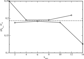
Figure 8: Increase of entropy for a system with constant heat capacity $C_{0}$ as a function the order of truncation of the asymptotic expansion $i_{max}$. The ratio of temperatures $T_{N}/T_{0}$ is equal to 2 and the number of reservoirs is $N=1$. The exact value corresponds to the dashed line.

In the table 2, we present more results of such calculations. We notice that quite accurate estimates of the entropy change may be obtained if the series is truncated at the most favorable order. The question of determining the order which minimizes the rest $R$ in the Euler-MacLaurin expansion Eq. (12) is rather technical and we refer to the specialized literature for details, but in general it may be assured that, if $f(x)$ in Eq. (12) has always the same sign and if the function and all its derivatives tend monotonically to $0$ as $x\to\infty$, which are valid for $f(N)=\Delta S(N)$, then the rest $R_{k_{max}}$ is of the same order and has the same sign of the first neglected term knopp .

$T_{N}/T_{0}$	$N$	$k_{max}$	$|\Delta S-\Delta S_{k_{max}}|/\Delta S$	$\Delta S$
$1/3$	$1$	$2$	$6.8311\times 10^{-2}$	$0.9014$
$1/3$	$2$	$6$	$4.3650\times 10^{-3}$	$0.4014$
$1/3$	$3$	$8$	$2.5634\times 10^{-4}$	$0.2538$
$1/3$	$4$	$12$	$1.2824\times 10^{-5}$	$0.1847$
$1/3$	$5$	$16$	$6.4910\times 10^{-7}$	$0.1450$
$1/3$	$6$	$18$	$3.0760\times 10^{-8}$	$0.1192$
$1/2$	$1$	$6$	$5.6735\times 10^{-3}$	$0.3069$
$1/2$	$2$	$12$	$1.6897\times 10^{-5}$	$0.1402$
$1/2$	$3$	$18$	$4.0671\times 10^{-8}$	$0.0765$
$2$	$1$	$6$	$9.0135\times 10^{-3}$	$0.1931$
$2$	$2$	$12$	$2.1570\times 10^{-5}$	$0.1098$
$2$	$3$	$18$	$4.7960\times 10^{-8}$	$0.0765$
$3$	$1$	$2$	$1.4255\times 10^{-1}$	$0.4319$
$3$	$2$	$6$	$6.6046\times 10^{-3}$	$0.2653$
$3$	$3$	$10$	$3.4783\times 10^{-4}$	$0.1907$
$3$	$4$	$12$	$1.5940\times 10^{-5}$	$0.1486$
$3$	$5$	$16$	$7.7345\times 10^{-7}$	$0.1217$
$3$	$6$	$18$	$3.5619\times 10^{-8}$	$0.1030$

Table 2: Body with constant heat capacity ($C(T)=C_{0}$). Values of the relative difference between the increase of entropy calculated directly ($\Delta S$) and the one which follows truncating the series Eq. (15) ($\Delta S_{k_{max}}$). Several values for $T_{N}/T_{0}$ and $N$ are considered, and the optimal order of truncation $i_{max}$ is given.

Finally, it is clear from Eq. (24) for the expansion coefficients, that for the case of a singular heat capacity at a critical temperature $T_{c}$ ($C(T)=C\tau(1-\tau)^{\alpha}$, with $\tau=T/T_{c}$), all but the first coefficients diverge if the temperature interval includes the critical temperature. This fact may account for the rather peculiar behavior found numerically in the large $N$ limit.

References

- (1) E. Fermi, Thermodynamics, Dover (1956).
- (2) R. Clausius, Annalen der Physik und Chemie, 125, 353 (1865), a translation may be found in William Francis Magie, A Source Book in Physics, McGraw-Hill (1935).
- (3) H. B. Callen, Thermodynamics and an introduction to thermostatistics, John Wiley & Sons (1985).
- (4) M. G. Calkin and D. Kiang, Am. J. Phys. 51, 78 (1983)
- (5) J. S. Thomsen and H. C. Bers, Am. J. Phys. 64, 580 (1996).
- (6) K. Knopp, Theorie und Anwendung der unendlichen Reihen, Springer Verlag, Berlin (1964).
- (7) The denominators and numerators of several Bernoulli numbers may be found in the addresses http://oeis.org/A027642 and http://oeis.org/A000367. respectively. These data are provided by the On Line Encyclopedia of Integer Sequences (http://oeis.org/wiki/Welcome).
- (8) J. Yeomans, Statistical Mechanics of Phase Transitions, (Oxford University Press (1992).