Universally optimal crossover designs under subject dropout

Abstract

Subject dropout is very common in practical applications of crossover designs. However, there is very limited design literature taking this into account. Optimality results have not yet been well established due to the complexity of the problem. This paper establishes feasible, as well as necessary and sufficient conditions for a crossover design to be universally optimal in approximate design theory in the presence of subject dropout. These conditions are essentially linear equations with respect to proportions of all possible treatment sequences being applied to subjects and hence they can be easily solved. A general algorithm is proposed to derive exact designs which are shown to be efficient and robust.

1 Introduction

Crossover designs have been widely used in industry due to their cost effectiveness and statistical efficiency. They are applicable for experiments aiming to compare effects of different treatments by applying them to a number of subjects across several periods. The response observation is typically modeled by additive effects of subjects, periods, treatments and the carryover effects of the treatment from the previous period. There has been tremendous amount of literature regarding the identification of optimal designs. See Hedayat and Afsarinejad (1978), Chêng and Wu (1980), Kunert (1984), Stufken (1991), Kushner (1997a, 1997b, 1998), Kunert and Martin (2000), Kunert and Stufken (2002), Hedayat and Yang (2003, 2004) and Hedayat and Zheng (2010), for instance. For comprehensive reviews, see Matthews (1988), Ratkowsky, Evans and Alldredge (1992), Stufken (1996), Jones and Kenward (2003), Senn (2003) and Bose and Dey (2009).

An important issue regarding crossover designs is that subject may drop out of the study. As a result, the experiment will not be carried out as planned. Matthews (1988) commented this is one of the main concerns of crossover designs. Low, Lewis and Prescott (1999) observed that “A dropout rate of between $5\%$ and $10\%$ is not uncommon and, in some areas, can be as high as $25\%$.” Meanwhile, a design, which is optimal or highly efficient in the absence of dropout, would become inefficient or even disconnected in the presence of subject dropout. Examples could be found in Godolphin (2004), Majumdar, Dean and Lewis (2008) as well as Section 5 of this paper.

To conclude, it is very important to find optimal or efficient designs in the presence of subject dropout, yet there is very limited literature on this. Bose and Bagchi (2008) derived designs which are universally optimal for both direct and carryover effects for both the situation of no dropout and the situation that all subjects drop out after period $q$ with $q$ being judiciously chosen. Similar results are presented by Majumdar, Dean and Lewis (2008). The latter restricted the comparison of designs within the subclass of uniformly balanced repeated measurement designs (UBRMDs), whose optimality property has been well recognized in literature for the situation of no dropout. For the second situation with any given $q$, they proposed type ${\mathcal{W}}_{q}$ UBRMDs, which reduce the maximum loss of the information for parameters in terms of $A$-criterion as compared to general UBRMDs. Following the latter paper, Zhao and Majumdar (2012) further explored the special case when $q$ is one less the number of periods and the numbers of treatments and periods are the same.

The previous three papers share two drawbacks: (i) The proposed designs exist only under very rare combinations of the numbers of subjects, periods and treatments. See Section 5.1.2 for relevant discussions of the former paper. As for the other two papers, it is well known that the existence of UBRMDs is rare. (ii) The information regarding the mechanism of how subjects drop out was not taken into account.

To address the latter drawback, it is plausible to measure the performance of designs by taking the expectation of a regular optimality criterion with respect to the mechanism of subject dropout. Low, Lewis and Prescott (1999) worked in this direction by using intensive computer programming. They concluded that when the Latin squares consisting of the design is more diverse, the resulting design performs better in terms of both efficiency and robustness. This argument is further supported by the comparison in Section 5. However, the case studies they provided fail to provide general guidance in identifying efficient designs. To serve this purpose, theoretical results are called for.

In this paper, we develop feasible equivalent conditions for a design to be universally optimal for direct treatment effects in approximate design theory under the same setup as that of Low, Lewis and Prescott (1999). The equivalence holds for any probability distribution of subject dropout. The results can be easily modified to find optimal or highly efficient exact designs for any combination of the numbers of subjects, periods and treatments. As a result, the two drawbacks are both addressed here.

The rest of the paper is organized as follows. Section 2 formulates the problem, introduces notation and gives some preliminary results. Section 3 introduces necessary concepts in approximate design theory, proves the existence of universally optimal designs and also gives necessary, sufficient and equivalent conditions for universal optimality. Section 4 gives explicit and feasible forms of optimality conditions in terms of linear equations, which are built upon the preceding section. Section 5 further provides a general algorithm for deriving an optimal or efficient exact design for any combination of the numbers of subjects, periods and treatments as well as any probability distribution of subject dropout. Besides, comparisons are made to designs in literature. Section 6 summarizes the results. Finally, some proofs are deferred to Section 7.

2 Framework

This section introduces the framework of the problem. Section 2.1 introduces the statistical model for the design problem and provides notation and assumptions necessary to the rest of the paper. Section 2.2 defines an ideal target function in finding a design, proposes a corresponding surrogate target function, and discusses the relationship between these two target functions. Section 2.3 provides some preliminary results as a preparation for the rest of the paper.

2.1 Modeling and notation

In a crossover design with $p$ periods, $t$ treatments and $n$ subjects, the response is typically modeled as

$$Y_{dku}=\mu+\pi_{k}+\varsigma_{u}+\tau_{d(k,u)}+\gamma_{d(k-1,u)}+\varepsilon_{ku},$$ (1)

where $\{\varepsilon_{ku},1\leq k\leq p,1\leq u\leq n\}$ are independent with mean zero and variance $\sigma^{2}$. Here, $Y_{dku}$ denotes the response from subject $u$ in period $k$ to which treatment $d(k,u)\in\{1,2,\ldots,t\}$ was assigned by design $d$. Furthermore, $\mu$ is the general mean, $\pi_{k}$ is the $k$th period effect, $\varsigma_{u}$ is the $u$th subject effect, $\tau_{d(k,u)}$ is the (direct) treatment effect of treatment $d(k,u)$ and $\gamma_{d(k-1,u)}$ is the carryover effect of treatment $d(k-1,u)$ that subject $u$ received in the previous period (by convention $\gamma_{d(0,u)}=0$).

Let $G$ be a temporary object whose meaning differs from context to context. Then we define $G^{\prime}$ to represent the transpose of the matrix $G$, $G^{-}$ to represent a generalized inverse of the matrix $G$, $\operatorname{tr}(G)$ to represent the trace of the matrix $G$ and $\operatorname{pr}^{\bot}$ to be a projection operator such that $\operatorname{pr}^{\bot}G=I-G(G^{\prime}G)^{-}G^{\prime}$. For two square matrices of equal size, $G_{1}$ and $G_{2}$, $G_{1}\leq G_{2}$ means that $G_{2}-G_{1}$ is nonnegative definite. For a set $G$, the number of elements in the set is represented by $|G|$.

Besides, $I_{k}$ is the $k\times k$ identity matrix, $1_{k}$ is the vector of length $k$ with all its entries as $1$, $J_{k}=1_{k}1_{k}^{\prime}$ is the square matrix with all its entries as $1$. We further define $B_{k}=I_{k}-J_{k}/k$, $B_{ij}^{k}$ to be the $i\times j$ matrix with its upper left corner filled with the submatrix $B_{k}$ while the remaining entries filled with $0$, and $B^{k}_{i}=B^{k}_{ii}$. The notation of $I_{ij}^{k}$ and $I_{i}^{k}$ are defined in the same fashions as $B_{ij}^{k}$ and $B_{i}^{k}$. Finally, $\otimes$ represents the Kronecker product of two matrices. To make the problem resolvable, it is necessary to make two mild assumptions as follows.

Assumption 1.

Once a subject drops out of the study, the probability that the subject reenters the study is zero.

By Assumption 1, we are able to define $l_{i}$, $1\leq i\leq n$, to be the total number of periods that subject $i$ stayed in the experiment. Further it is realistic in a large number of applications to assume the following:

Assumption 2.

The dropping out mechanism is independent of the choice of design $d$ as well as the outcome of the experiments. Moreover $\{l_{i},1\leq i\leq n\}$ are i.i.d.

By Assumption 2, we could define $a_{k}$ to be the probability that $l_{i}=k$, $1\leq k\leq p$, and hence we are in place to define the following technical terms:

• $\vec{a}=(a_{1},a_{2},\ldots,a_{p})$.

• $a_{jk}=\sum^{k}_{i=j}a_{i}$, $1\leq j\leq k\leq p$. (Convention: $a_{p+1,p}=0$.)

• $m=\min\{k\dvtx a_{k}>0\}$.

• $\alpha_{k}=n^{-1}((n+1)a_{k}+a_{1,k-1}^{n+1}-a_{1k}^{n+1})$, $1\leq k\leq p$.

• $\beta_{k}=a_{k}+a_{k+1,p}a_{1k}^{n}-a_{kp}a_{1,k-1}^{n}$, $1\leq k\leq p$.

• $A=\sum^{p}_{k=1}\alpha_{k}B^{k}_{p}$.

• $B=\sum^{p}_{k=1}\beta_{k}B^{k}_{p}$.

Definition 1.

An experiment is said to be complete if there is no dropout.

By definition the complete experiment is a special case in our framework and has been extensively studied in literature. Here, we aim to investigate desirable designs for any given dropout mechanism $\vec{a}$.

Notice that $A$ and $B$ are both nonnegative definite matrices. Since $\beta_{k}\geq a_{k}+a_{k+1,p}a_{1k}^{n}-a_{kp}a_{1k}^{n}=a_{k}(1-a_{1k}^{n})\geq 0$, we have $B\geq 0$. By the mean value theorem one could show that $\alpha_{k}\geq 0$ and hence $A\geq 0$. Note that $a_{k}=0$ implies $\alpha_{k}=\beta_{k}=0$. Hence we have $A=\sum^{p}_{k=m}\alpha_{k}B^{k}_{p}$ and $B=\sum^{p}_{k=m}\beta_{k}B^{k}_{p}$. The same representation will be adopted in the sequel whenever the summation over the period $k$ is involved. Finally, we should be aware of the differences and relationships among the matrices $B_{k}$, $B^{k}_{p}$ and $B$.

2.2 Optimality criteria

Writing the $np\times 1$ response vector as ${Y}_{d}=(Y_{d11},Y_{d21},\ldots,Y_{dp1},Y_{d12},\ldots,Y_{dpn})^{\prime}$, model (1) can be written as

$$Y_{d}={1}_{np}\mu+Z\bolds{\pi}+U\bolds{\varsigma}+{T}_{d}\bolds{\tau}+{F}_{d}\bolds{\gamma}+\varepsilon,$$ (2)

where $\bolds{\pi}=(\pi_{1},\ldots,\pi_{p})^{\prime}$, $\bolds{\varsigma}=(\varsigma_{1},\ldots,\varsigma_{n})^{\prime}$, $\bolds{\tau}=(\tau_{1},\ldots,\tau_{t})^{\prime}$, $\bolds{\gamma}=(\rho_{1},\ldots,\rho_{t})^{\prime}$, $Z={1}_{n}\otimes{I}_{p}$, $U=I_{n}\otimes 1_{p}$ and ${T}_{d}$ and ${F}_{d}$ denote the treatment/subject and carryover/subject incidence matrices. Here ${\mathbb{E}}\varepsilon=0$ and $\operatorname{Var}(\varepsilon)=\sigma^{2}I_{np}$. For design $d$ under a realization of experiment $l=(l_{1},\ldots,l_{n})^{\prime}$, the information matrix for the direct treatment effects $\tau$ under model (2) with $\sigma^{2}=1$ is

$$C_{d}(\tau,l) = (MT_{d})^{\prime}\operatorname{pr}^{\bot}(MZ|MU|MF_{d})(MT_{d})$$

$$= C_{d11}(l)-C_{d12}(l)\bigl{[}C_{d22}(l)\bigr{]}^{-}C_{d21}(l),$$

where

$$C_{d11}(l) = T_{d}^{\prime}OT_{d},\qquad C_{d12}(l)=T_{d}^{\prime}OF_{d},$$

$$C_{d21}(l) = C_{d12}^{\prime},\qquad C_{d22}(l)=F_{d}^{\prime}OF_{d},$$

$$M = \operatorname{diag}\bigl{(}I_{l_{i},p}^{l_{i}},i=1,2,\ldots,n\bigr{)},$$

$$O = M^{\prime}\operatorname{pr}^{\bot}(MZ|MU)M.$$

Under a complete experiment, Kiefer (1975) defined a design to be universally optimal if it maximizes $\Phi(C_{d}(\tau,p1_{n}))$ for any $\Phi$ satisfying: [(C.1)]

$\Phi$ is concave;

$\Phi(S^{\prime}CS)=\Phi(C)$ for any permutation matrix $S$;

$\Phi(bC)$ is nondecreasing in the scalar $b>0$.

Optimality criteria defined by such a $\Phi$ includes, but is not limited to, $A$, $D$, $E$ and $T$. See Kiefer (1975) and Yeh (1986) for instance. In the subject dropout setup there does not exist a design which maximizes $\Phi(C_{d}(\tau,l))$ for all realizations of $l$. One reasonable target is to find a design which maximizes $\phi_{0}(d|\Phi,\vec{a}):={\mathbb{E}}_{\vec{a}}\Phi(C_{d}(\tau,l))$ for any $\Phi$ satisfying the above three conditions. Here the expectation is taken over the probability space of $l$ with parameter $\vec{a}$. For notational simplicity, we would omit the subscript $\vec{a}$ for ${\mathbb{E}}$ and the parameters $\Phi$ and $\vec{a}$ for $\phi_{0}$ whenever it is clear from the context. So we have $\phi_{0}(d):=\phi_{0}(d|\Phi,\vec{a})={\mathbb{E}}\Phi(C_{d}(\tau,l))$.

There are two major difficulties in maximizing $\phi_{0}(d)$ which make the problem intractable, if not impossible: (i) $\Phi$ is a nonlinear function and hence the expectation would interact with the form of $\Phi$. (ii) Even when the dropout situation $l$ is fixed, there is still a lack of tools to deal with the information matrix $C_{d}(\tau,l)$ if subjects drop out at different periods under $l$. In order to tackle these difficulties, we propose to replace the original target function of $\phi_{0}(d)$ with the surrogate target function of $\phi_{1}(d)=\Phi(C_{d})$ where

$$C_{d} = C_{d11}-C_{d12}C_{d22}^{-}C_{d21},$$

$$C_{dij} = {\mathbb{E}}C_{dij}(l),\qquad 1\leq i,j\leq 2.$$

It will be shown in Section 5 that this replacement is very successful in identifying highly efficient, if not optimal, designs for the criterion $\phi_{0}(d)$.

For $i=0$ or $1$, let $d^{*}_{i}$ be an optimal design under $\phi_{i}$. Then define $e_{i}(d)=\phi_{i}(d)/\phi_{i}(d^{*}_{i}),i=0,1$, to be the efficiency of $d$ under $\phi_{i}$-criterion. Also we call $g(d)=\phi_{0}(d)/\phi_{1}(d)$ to be the gap function between the two target functions for design $d$. Even though we are working on $\phi_{1}$ instead of $\phi_{0}$, the $\phi_{0}$-efficiency $e_{0}(d)$ could be bounded by $e_{1}(d)g(d)$ as shown by Lemma 2.

Lemma 1 ([Pukelsheim (1993), pages 74–77]).

The Schur complement of a matrix $G\geq 0$ is a concave nondecreasing function of $G$.

Lemma 2.

For any $\Phi$, $\vec{a}$ and design $d$, we have $\phi_{0}(d)\leq\phi_{1}(d)$. Further we have

$$e_{0}(d)\geq e_{1}(d)g(d).$$

In particular, for any $\phi_{1}$-optimal design $d$, we have $e_{0}(d)\geq g(d)$.

By Lemma 1 we have ${\mathbb{E}}C_{d}(\tau,l)\leq C_{d}$. Then we have

$$\phi_{0}(d) = {\mathbb{E}}\Phi\bigl{(}C_{d}(\tau,l)\bigr{)}$$ (4)

$$\leq \Phi\bigl{(}{\mathbb{E}}C_{d}(\tau,l)\bigr{)}$$

$$\leq \Phi(C_{d})$$ (5)

$$= \phi_{1}(d).$$ (6)

By (6) we have $e_{0}(d)=\phi_{0}(d)/\phi_{0}(d^{*}_{0})\geq\phi_{0}(d)/\phi_{1}(d^{*}_{0})\geq\phi_{0}(d)/\phi_{1}(d^{*}_{1})=\break e_{1}(d)g(d).$

By (6) we have $g(d)\leq 1$, and hence $g(d_{1}^{*})\leq e_{0}(d^{*}_{1})$. That means if we could find a $\phi_{1}$-optimal design, then the value of the gap function $g$ evaluated at this design serves as a lower bound of its $\phi_{0}$-efficiency. Inequalities (4) and (5) are essentially Jensen-type inequalities. The equalities therein both hold if the realization of subject dropout, $l$, is not random. When the variation in $l$ is not very large, it would be plausible to work on the surrogate target of maximizing $\phi_{1}(C_{d})$ instead of $\phi_{0}(C_{d})$ since the value of the gap function $g$ would be close to unity. Note that a popular choice of $\Phi$ is the trace of a matrix ($T$-criterion), for which the equality in (4) always holds.

When the experiment is complete, the necessary and sufficient conditions for $\phi_{1}$-universal optimality derived in Section 4 reduce to that of Kushner (1997b). Note that the matrix $C_{d}$ in (2.2) is no longer an information matrix for any design, and as a result the ideas of proving the existence of universally optimal designs, given by Theorem 3.4 of Kushner (1997b), are not applicable here. However, we found that similar results could be derived by direct manipulation on the matrix $C_{d}$. See Sections 3.2 and 3.3 for details. Moreover, since $A\neq B$ in general, the arguments in deriving the linear equation as in proof of Theorem 5.3 of Kushner (1997b) are not applicable here either. For the approach of tackling this difficulty, see Section 4.1 for details.

2.3 Preliminary results

Lemma 3.

Under Assumptions 1 and 2 we have $C_{d11}=T_{d}^{\prime}VT_{d}$, $C_{d12}=T_{d}^{\prime}VF_{d}$ and $C_{d22}=F_{d}^{\prime}VF_{d}$ with

$$V = \sum^{p}_{k=m}\bigl{(}\alpha_{k}I_{n}-n^{-1}\beta_{k}J_{n}\bigr{)}\otimes B^{k}_{p}$$

$$= I_{n}\otimes A-n^{-1}J_{n}\otimes B.$$

Since $B^{1}_{p}=0$ the $m$ in (3) could be replaced by $\operatorname{max}(m,2)$. A heuristic explanation for this observation is that when $l_{i}=1$ there is no information gained from this subject, because we rely on within subject comparison for treatments in crossover designs. When the experiment is complete we have $\alpha_{k}=\beta_{k}=0$ for all $1\leq k\leq p-1$ and $\alpha_{p}=\beta_{p}=1$. In this case, we have the reduction of $A=B=B_{p}$ and $V=B_{n}\otimes B_{p}$, for which the optimality problem has been extensively studied in literature.

Corollary 1.

Any design which is $\phi_{1}$-optimal with $\Phi$ satisfying conditions (C.1)–(C.3) under model (1) is still optimal under the same criterion when the within subject covariance is of the form

$$\Sigma=I_{p}+\eta 1_{p}^{\prime}+1_{p}\eta^{\prime}.$$ (8)

One special case is the compound symmetric covariance matrix, that is, $\Sigma=I_{p}+bJ_{p}$. Here $\eta$ is an arbitrary vector, and $b$ is an arbitrary real number.

Let $\Sigma_{k}$ be the $k\times k$ upper left submatrix of $\Sigma$ for $1\leq k\leq p$. By direct calculation, we have

$$\Sigma_{k}^{-1}-\Sigma_{k}^{-1}J_{k}\Sigma_{k}^{-1}/1_{k}^{\prime}\Sigma_{k}^{-1}1_{k}=B_{k}.$$ (9)

By following the same calculation as the proof of Lemma 3, the corollary is established in view of equation (9).

Remark 1.

The covariance matrix as in (8) is called a “type-H” matrix; see Huynh and Feldt (1970).

3 $\phi_{1}$-universal optimality

This section explores the $\phi_{1}$-universal optimality in approximate design theory, where $\phi_{1}$-universal optimality is defined as follows.

Definition 2.

Given $p$, $t$, $n$ and a dropout mechanism $\vec{a}$, a design $d$ is said to be $\phi_{1}$-universally optimal if $d$ maximizes $\phi_{1}(d)$ over all designs for any $\Phi$ satisfying conditions (C.1), (C.2) and (C.3).

Section 3.1 introduces the ideas in approximate design theory as well as the concept of symmetric designs. Section 3.2 shows that a design would be $\phi_{1}$-universally optimal as long as its information matrix is of the form $C_{d}=ny^{*}B_{t}/(t-1)$ with $y^{*}$ introduced by equation (14). Section 3.3 shows that there always exists a symmetric design which satisfies this sufficient condition for $\phi_{1}$-universal optimality, and further by argument of Kiefer (1975) that this condition is also necessary for any design to be $\phi_{1}$-universally optimal. However, this condition is not immediately applicable for application. Section 4 gives an equivalent condition which is more readily applicable. Some relevant technical preparations are given in Sections 3.4 and 3.5.

3.1 Approximate design theory and symmetric designs

A design $d$ with $p$ periods, $t$ treatments and $n$ subjects could be considered as the result of selecting $n$ sequences with replacement from the collection of all possible $t^{p}$ sequences, and this collection is denoted by ${\mathcal{S}}$. Let $n_{s}$ be the number of replications of sequence $s$ in the design, and define $P_{d}=(p_{s},s\in{\mathcal{S}})$ with $p_{s}=n_{s}/n$. When we ignore the ordering of the $n$ sequences in the design, we have the one to one correspondence of $d\leftrightarrow(n,P_{d})$ with the restrictions of (i) $\sum_{s\in{\mathcal{S}}}p_{s}=1$, (ii) $p_{s}\geq 0$ and (iii) $np_{s}$ being an integer for all $s$. In approximate design theory, we only keep the first two restrictions and allow $np_{s}$ not to be an integer.

Let $\sigma$ be a permutation of symbols $\{1,2,\ldots,t\}$. For a sequence $s=(t_{1},\ldots,\break t_{p})$, we define $\sigma s=(\sigma(t_{1}),\ldots,\sigma(t_{p}))$. Then the design $\sigma d$ is defined by $P_{\sigma d}=(p_{\sigma^{-1}s},s\in{\mathcal{S}})$. The permutation matrix $S_{\sigma}$ is the unique matrix satisfying $T_{\sigma s}=T_{s}S_{\sigma}$ for all $s\in{\mathcal{S}}$. In the sequel we replace the subject index $u$ by sequence index $s$ whenever it is necessary.

A design $d$ is said to be symmetric if $P_{d}=P_{\sigma d}$. Also we define symmetric blocks as $\langle s\rangle=\{\sigma s,\sigma\in{\mathcal{P}}\}$ where ${\mathcal{P}}$ is the collection of all possible $t!$ permutations, that is, $|{\mathcal{P}}|=t!$. We further define $p_{\langle s\rangle}=\sum_{\tilde{s}\in\langle s\rangle}p_{\tilde{s}}$. For a symmetric design, we have $p_{\tilde{s}}=p_{\langle s\rangle}/|\langle s\rangle|$ for any $\tilde{s}\in\langle s\rangle$. Given $p,t,n$, a symmetric design $d$ is uniquely determined by $(p_{\langle s\rangle},s\langle\in\rangle{\mathcal{S}})$, where $s\langle\in\rangle{\mathcal{S}}$ means that $s$ runs through all distinct symmetric blocks contained in ${\mathcal{S}}$.

3.2 A sufficient condition for $\phi_{1}$-universal optimality

Denote by $T_{u}$ (resp., $F_{u}$) the $p\times t$ submatrix of $T$ (resp., $F$) corresponding to the $u$th subject. Define $\overline{T}=n^{-1}\sum^{n}_{u=1}T_{u}$, $\hat{T}_{u}=T_{u}B_{t}$ and $\hat{\overline{T}}=\overline{T}B_{t}$. The notation $\overline{F}$, $\hat{F}_{u}$ and $\hat{\overline{F}}$ are defined in the same way corresponding to carryover effects. Let $\overline{C}_{dij}=\sum_{\sigma\in{\mathcal{P}}}S_{\sigma}^{\prime}C_{dij}S_{\sigma}/|{\mathcal{P}}|$, $1\leq i,j\leq 2$ and $\overline{C}_{d}=\sum_{\sigma\in{\mathcal{P}}}S_{\sigma}^{\prime}C_{d}S_{\sigma}/|{\mathcal{P}}|$. Note that $\overline{C}_{dij},1\leq i,j\leq 2$, are completely symmetric, also $\overline{C}_{d11}$ and $\overline{C}_{d12}=(\overline{C}_{d21})^{\prime}$ have row and column sums as zero. Let $\mathbb{I}$ be the indicator function. By Proposition 1 of Kunert and Martin (2000), we have

$$\overline{C}_{d} \leq \tilde{C}_{d}$$ (10)

$$= \biggl{(}c_{d11}-\frac{c_{d12}^{2}}{c_{d22}}\mathbb{I}_{[c_{d22}>0]}\biggr{)}\frac{B_{t}}{t-1},$$ (11)

where

$$\tilde{C}_{d} = \overline{C}_{d11}-\overline{C}_{d12}(\overline{C}_{d22})^{-}\overline{C}_{d21},$$

$$c_{dij} = \operatorname{tr}(B_{t}\overline{C}_{dij}B_{t})=\operatorname{tr}(B_{t}C_{dij}B_{t}),\qquad 1\leq i,j\leq 2.$$

Define $\hat{C}_{dij}=\sum^{n}_{u=1}\hat{C}_{uij}$, where $\hat{C}_{uij}=G_{i}^{\prime}AG_{j}$ with $G_{1}=\hat{T}_{u}$ and $G_{2}=\hat{F}_{u}$. Since $B\geq 0$, we have

$$(B_{t}C_{dij}B_{t})_{1\leq i,j\leq 2} = \pmatrix{\hat{C}_{d11}&\hat{C}_{d12}\vspace*{2pt}\cr\hat{C}_{d21}&\hat{C}_{d22}}-n\pmatrix{\hat{\overline{T}}{}^{\prime}_{d}\vspace*{2pt}\cr\hat{\overline{F}}{}^{\prime}_{d}}B\pmatrix{\hat{\overline{T}}_{d}&\hat{\overline{F}}_{d}}$$

$$\leq (\hat{C}_{dij})_{1\leq i,j\leq 2}.$$

Define $q_{dij}=\operatorname{tr}(\hat{C}_{dij})$ and $q_{uij}=\operatorname{tr}(\hat{C}_{uij})$. Then we have $q_{dij}=\sum^{n}_{u=1}q_{uij}$. It is easy to see that $q_{u22}>0$ and hence $q_{d22}>0$, which allow us to define

$$q_{d}^{*}=q_{d11}-\frac{q_{d12}^{2}}{q_{d22}}.$$

By (3.2) we have

$$\pmatrix{c_{d11}&c_{d12}\vspace*{2pt}\cr c_{d21}&c_{d22}}\leq\pmatrix{q_{d11}&q_{d12}\vspace*{2pt}\cr q_{d21}&q_{d22}},$$

and then by Lemma 1 we have

$$c_{d11}-\frac{c_{d12}^{2}}{c_{d22}}\mathbb{I}_{[c_{d22}>0]}\leq q_{d}^{*},$$ (13)

with the equality holds when $\hat{\overline{T}}_{d}=\hat{\overline{F}}_{d}=0$. The latter is achieved by designs which are uniform on periods. To introduce the following theorem, we define

$$y^{*}=\frac{1}{n}\max_{d}q_{d}^{*}.$$ (14)

Theorem 1

If $C_{d}=ny^{*}B_{t}/(t-1)$ with $y^{*}$ defined in (14), then the design $d$ is $\phi_{1}$-universally optimal.

By conditions (C.1) and (C.2) of $\Phi$ we have

$$\Phi(C_{d})\leq\Phi(\overline{C}_{d}),$$ (15)

where the equality holds if $C_{d}$ is completely symmetric, that is, $C_{d}=\operatorname{tr}(C_{d})B_{t}/(t-1)$ since $C_{d}$ has row and column sums as zero. The theorem is proved in view of (10), (11), (13), (14), (15) and condition (C.3).

3.3 Existence and equivalence

Theorem 1 provides a sufficient condition for a design to be $\phi_{1}$-universally optimal. A natural question is the following: does there exist such a design? This section gives a positive answer as well as its corresponding implications.

Theorem 2

For any symmetric design, we have: [(1)]

$C_{d}$ is completely symmetric;

$\operatorname{tr}(C_{d})=q_{d}^{*}$;

given any design $d$ there always exist a corresponding symmetric design which has the same value of $q_{d}^{*}$.

Remark 2.

Note that Theorem 2 does not hold if we replace $C_{d}$ therein by $C_{d}(\tau,l)$. Hence the argument cannot be applied to $\Phi(C_{d}(\tau,l))$ directly. This is why we work on $\phi_{1}$ instead of $\phi_{0}$ directly.

Corollary 2.

(i) There exists a symmetric $\phi_{1}$-universally optimal design $d$ with

$$C_{d}=\frac{ny^{*}B_{t}}{t-1}.\vspace*{-6pt}$$ (16)

If a design $d$ is $\phi_{1}$-universally optimal (or $\phi_{1}$-optimal with $\Phi$ strictly concave or increasing), then we have (16).

(i) is proved by Theorems 1 and 2. (ii) is proved by (i) and the remark in Kiefer’s (1975) Proposition 1.

3.4 A necessary condition for $\phi_{1}$-universal optimality

In this section we give a necessary condition for a design to be $\phi_{1}$-universally optimal and define quantities that will be useful for presenting the necessary and sufficient conditions for $\phi_{1}$-universal optimality in Section 4. Now define the function $q_{s}(x)=q_{s11}+2q_{s12}x+q_{s22}x^{2}$ and $q_{d}(x)=q_{d11}+2q_{d12}x+q_{d22}x^{2}$. Since $q_{dij}=\sum^{n}_{u=1}q_{uij}=n\sum_{s\in{\mathcal{S}}}p_{s}q_{sij}$ we have

$$q_{d}(x)=n\sum_{s\in{\mathcal{S}}}p_{s}q_{s}(x).$$ (17)

Since $q_{d22}>0$, by direct calculation we have

$$q_{d}^{*} = \min_{x}q_{d}(x)$$

$$= n\min_{x}\sum_{s\in{\mathcal{S}}}p_{s}q_{s}(x).$$

By (14) and (3.4) we have

$$y^{*}=\max_{P}\min_{x}\sum_{s\in{\mathcal{S}}}p_{s}q_{s}(x).$$ (19)

Let $d^{*}$ be a design which maximizes $q^{*}_{d}$. By (17), (3.4) and (19) we have $\min_{x}q_{d^{*}}(x)=q^{*}_{d^{*}}=ny^{*}$. Since $q_{d22}>0$ the equation $q_{d^{*}}(x)=ny^{*}$ has a unique solution which is denoted by $x^{*}$. Define

$${\mathcal{T}}=\bigl{\{}s\in{\mathcal{S}}\dvtx y^{*}=q_{s}\bigl{(}x^{*}\bigr{)}\bigr{\}}.$$

Lemma 4 shows that any universally optimal design is supported on ${\mathcal{T}}$.

Lemma 4.

If a design $d$ is $\phi_{1}$-universally optimal (or $\phi_{1}$-optimal with $\Phi$ strictly concave or increasing) then we have

$$p_{s}=0,\qquad s\notin{\mathcal{T}}.$$

By Corollary 2, we have $\operatorname{tr}(C_{d})=ny^{*}$ and $C_{d}=\overline{C}_{d}$. By (10), (11) and (13) we have $\operatorname{tr}(\overline{C}_{d})\leq q^{*}_{d}$. The theorem is proved in view of (14) and Section 4.4 of Kushner (1997b).

3.5 Determination of $x^{*}$, $y^{*}$ and ${\mathcal{T}}$

For a sequence $s=(t_{1},t_{2},\ldots,t_{p})$, define $s_{k}=(t_{1},\ldots,t_{k})$ to be the first $k$ periods of $s$. Particularly, we have $s=s_{p}$. For $1\leq k\leq p$ and $1\leq i\leq t$, we define the treatment/sequence index $f_{s_{k},i}=\sum^{k}_{j=1}1_{t_{j}=i}$. To introduce the following theorem, we define two special symmetric blocks. The symmetry block $\langle di\rangle$ consists of all sequences having distinct treatments in the $p$ periods. The symmetry block $\langle re\rangle$ consists of all sequences having distinct treatments in the first $p-1$ periods, with the treatment in period $p-1$ repeating in period $p$.

Theorem 3

For any integer $k>t$, define $z_{k}$ and $r_{k}$ to be integers satisfying $k=z_{k}t+r_{k}$ and $0<r_{k}\leq t$. [(iii)]

If $m>t$ and

$$\sum^{p}_{k=m}\alpha_{k}\bigl{[}k\bigl{(}mt-t^{2}+1-k\bigr{)}+t-r_{k}(t-r_{k}+1)\bigr{]}\geq 0,$$ (20)

then

$$x^{*} = 0,$$

$$y^{*} = \sum^{p}_{k=m}\alpha_{k}\bigl{[}k(1-1/t)-r_{k}(t-r_{k})/pt\bigr{]},$$

$${\mathcal{T}} = \{s\dvtx f_{s_{k},i}=z_{k}\mbox{ or }z_{k}+1,1\leq i\leq t,m\leq k\leq p\}.$$

If $p\leq t$ and

$$\sum^{p-1}_{k=m}\alpha_{k}(k-1)(p+1/t-k)\leq\alpha_{p}\bigl{[}(p-1)^{2}-(1+1/t)p+1/t\bigr{]},$$ (21)

then

$$x^{*} = 1/(p-1),$$

$$y^{*} = \sum^{p}_{k=m}\alpha_{k}(k-1)\biggl{(}1-\frac{2p-1-k+1/t}{k(p-1)^{2}}\biggr{)},$$

$${\mathcal{T}} = \langle re\rangle\cup\langle di\rangle.$$

When the two sides of (21) are equal, we have ${\mathcal{T}}=\langle re\rangle$.

Let

$$x_{0}=\frac{\sum^{p-1}_{k=m}\alpha_{k}(k-1)}{\sum^{p}_{k=m}\alpha_{k}(k-1)(k-1-1/t)}.$$

If $(p-1)^{-1}<x_{0}<(p-2)^{-1}$, then

$$x^{*} = x_{0},$$

$$y^{*} = \sum^{p}_{k=m}\alpha_{k}(k-1)(1-1/k-1/kt)x^{2}_{0}-2\sum^{p-1}_{k=m}\alpha_{k}(1-1/k)x_{0}$$

$${}+\sum^{p}_{k=m}\alpha_{k}(k-1)-2/p,$$

$${\mathcal{T}} = \langle re\rangle.$$

Remark 3.

Under complete experiment, Theorem 3(i) applies to the case $p>t$, and Theorem 3(ii) applies to the case $p\leq t$. Actually Theorem 3(i), (ii) reduce to Theorem 1 of Kushner (1998). One can extrapolate by continuity that Theorem 3(i), (ii) cover the cases when the dropout issue is not very serious.

Remark 4.

When $m=p-1$, we would also discuss parts (i) and (ii) of Theorem 3. For (i), a sufficient condition for (20) is $p>t+3$. For (ii), inequality (21) simplifies to

$$\alpha_{p}\geq\frac{(p-2)(1+1/t)}{(p-1)^{2}-2-1/t}.$$ (22)

The right-hand side of (22) mainly depends on $p$, and it will become very small for large $p$. Particularly, a sufficient condition for (22) is

$$a_{p}\geq\frac{n}{n+1}\frac{(p-2)(1+1/t)}{(p-1)^{2}-2-1/t}+\frac{1}{n+1}.$$

4 Linear equations for $\phi_{1}$-universal optimality

Built upon the results of Section 3, this section provides feasible equivalent conditions in approximate design theory for $\phi_{1}$-universal optimality.

4.1 Equations for general designs

Recall that $\hat{T}_{u}=T_{u}B_{t}$ and $\hat{F}_{u}=F_{u}B_{t}$, and then we define

$$\check{C}_{d} = \check{C}_{d11}-\check{C}_{d12}\check{C}_{d22}^{-}\check{C}_{d21},$$

$$\check{C}_{dij} = \sum^{n}_{u=1}\check{C}_{uij},\qquad 1\leq i,j\leq 2,$$

where

$$\check{C}_{u11} = T_{u}^{\prime}(A-B)T_{u}+\hat{T}_{u}^{\prime}B\hat{T}_{u},\qquad\check{C}_{u12}=T_{u}^{\prime}(A-B)F_{u}+\hat{T}_{u}^{\prime}B\hat{F}_{u},$$

$$\check{C}_{u21} = \check{C}_{u12}^{\prime},\qquad\check{C}_{u22}=F_{u}^{\prime}(A-B)F_{u}+\hat{F}_{u}^{\prime}B\hat{F}_{u}.$$

We shall replace $\check{C}_{uij}$ with $\check{C}_{sij}$ in emphasizing sequence $s$ instead of subject $u$ of a design. By direct calculation we have

$$\check{C}_{dij}=C_{dij}+nG_{i}^{\prime}BG_{j},\qquad 1\leq i,j\leq 2,$$ (24)

where $G_{1}=\hat{\overline{T}}_{d}$ and $G_{2}=\hat{\overline{F}}_{d}$. The following lemma is crucial for the proof of Theorem 4.

Lemma 5.

If $d$ is $\phi_{1}$-universally optimal (or $\phi_{1}$-optimal with $\Phi$ strictly concave or increasing), we have $C_{d}=\check{C}_{d}=ny^{*}B_{t}/(t-1)$.

By (24) and Lemma 1 we have

$$C_{d}\leq\check{C}_{d}.$$ (25)

By Corollary 2(ii) we have

$$C_{d}=ny^{*}B_{t}/(t-1).$$ (26)

Let $\bar{d}$ be the symmetrized version of design $d$ as defined by (59), and then by (4.1) we have

$$\sum_{\sigma\in{\mathcal{P}}}S_{\sigma}^{\prime}\check{C}_{dij}S_{\sigma}/|{\mathcal{P}}|=\check{C}_{\bar{d}ij}.$$ (27)

Again by (24) we have $\check{C}_{dij}=G_{i}^{\prime}\Lambda G_{j}$ with $G_{1}=(\hat{\overline{T}}{}^{\prime}_{d},T_{d}^{\prime})^{\prime}$, $G_{2}=(\hat{\overline{F}}{}^{\prime}_{d},F_{d}^{\prime})^{\prime}$, and

$$\Lambda=\pmatrix{nB&0\vspace*{2pt}\cr 0&V}.$$

Since $\Lambda\geq 0$ we have by Proposition 1 of Kunert and Martin (2000) that

$$\sum_{\sigma\in{\mathcal{P}}}S_{\sigma}^{\prime}\check{C}_{d}S_{\sigma}/|{\mathcal{P}}|\leq\check{C}_{\bar{d}},$$ (28)

in view of (27). Since $\hat{\overline{T}}_{\bar{d}}=\hat{\overline{F}}_{\bar{d}}=0$ for the symmetric design $\bar{d}$, we have

$$\check{C}_{\bar{d}}=C_{\bar{d}}.$$ (29)

Combining (25)–(28) and (29), we have

$$\frac{ny^{*}}{t-1}B_{t}=C_{d} = \overline{C}_{d}$$

$$\leq \sum_{\sigma\in{\mathcal{P}}}S_{\sigma}^{\prime}\check{C}_{d}S_{\sigma}/|{\mathcal{P}}|$$

$$\leq C_{\bar{d}}.$$

Hence we have $C_{\bar{d}}=ny^{*}B_{t}/(t-1)$ in view of Corollary 2 and thus

$$\sum_{\sigma\in{\mathcal{P}}}S_{\sigma}^{\prime}\check{C}_{d}S_{\sigma}/|{\mathcal{P}}|=ny^{*}B_{t}/(t-1),$$

which in turn yields

$$\operatorname{tr}(\check{C}_{d})=ny^{*}.$$ (30)

The lemma is now proved in view of (25) and (30).

Theorem 4

A design $d$ is $\phi_{1}$-universally optimal (or $\phi_{1}$-optimal with $\Phi$ strictly concave or increasing) if and only if

$$\sum_{s\in{\mathcal{T}}}p_{s}\bigl{[}\check{C}_{s11}+x^{*}\check{C}_{s12}B_{t}\bigr{]} = \frac{y^{*}}{t-1}B_{t},$$ (31)

$$\sum_{s\in{\mathcal{T}}}p_{s}\bigl{[}\check{C}_{s21}+x^{*}\check{C}_{s22}B_{t}\bigr{]} = 0,$$ (32)

$$\sum_{s\in{\mathcal{T}}}p_{s}B\bigl{(}\hat{T}_{s}+x^{*}\hat{F}_{s}\bigr{)} = 0,$$ (33)

$$\sum_{s\in{\mathcal{T}}}p_{s} = 1,$$ (34)

$$p_{s} = 0,\qquad s\notin{\mathcal{T}}.$$ (35)

Based on Theorem 1 and Corollary 2, (16) is also a necessary and sufficient condition for $\phi_{1}$-universal optimality. However, (16) is not directly applicable for identifying designs. Note that the conditions in Theorem 4 are merely linear equation systems for $p_{s}$, and hence can be easily implemented to derive exact designs. See Section 5.

4.2 Equations for symmetric designs

Note that $q_{s}(x)$ is invariant to treatment permutation, that is,

$$q_{s}(x)=q_{\sigma s}(x).$$ (36)

Combining Theorem 4.5 of Kushner (1997b), Theorem 2, Corollary 2, Lemma 4 and equation (36), we have the following:

Theorem 5

A symmetric design is $\phi_{1}$-universally optimal if

$$\sum_{s\langle\in\rangle{\mathcal{T}}}p_{\langle s\rangle}q_{s}^{\prime}\bigl{(}x^{*}\bigr{)} = 0,$$

$$\sum_{s\langle\in\rangle{\mathcal{T}}}p_{\langle s\rangle} = 1,$$

$$p_{s} = 0,\qquad s\notin{\mathcal{T}},$$

where $q_{s}^{\prime}(x)$ is the derivative of $q_{s}(x)$ with respective to $x$.

5 Exact designs

This section gives algorithms to identify efficient exact designs based on the optimality equations in Section 4. Results are compared to designs proposed in literature. For the matrix $C_{d}(\tau,l)$, denote its eigenvalues by $0=\lambda_{1}\leq\lambda_{2}\leq\cdots\leq\lambda_{t}$. We define the criteria of $A$, $D$, $E$ and $T$ as:

• $\Phi_{A}(C_{d}(\tau,l))=(t-1)(n\sum^{t}_{i=2}\lambda_{i}^{-1})^{-1}$. [$\lambda_{2}=0$ implies $\Phi_{A}(C_{d}(\tau,l))=0$];

• $\Phi_{D}(C_{d}(\tau,l))=n^{-1}(\prod^{t}_{i=2}\lambda_{i})^{1/(t-1)}$;

• $\Phi_{E}(C_{d}(\tau,l))=n^{-1}\lambda_{2}$;

• $\Phi_{T}(C_{d}(\tau,l))=[n(t-1)]^{-1}(\sum^{t}_{i=2}\lambda_{i})$.

Section 5.1 provides an algorithm to derive exact designs for general configurations of $p,t,n$. Section 5.2 illustrates how to derive symmetric designs by straightforward calculations. In utilizing Lemma 2, $e_{1}(d)$ is further bounded by $\tilde{e}_{1}=\phi_{1}(d)/\phi_{1}(\tilde{d})$, where $\tilde{d}$ is a $\phi_{1}$-optimal design in asymptotic design theory which may not necessarily exist as an exact design. Thus the function $\ell(d)=\tilde{e}_{1}(d)g(d)$ serves as a feasible lower bound of $e_{0}(d)$.

5.1 General exact designs

This section gives an algorithm to derive efficient exact optimal designs for any given configuration of $p,t,n$ and compares them to designs in literature. Note that the latter designs are proposed for judiciously chosen $p,t,n$ while our algorithm works for any configuration of $p,t,n$. Even under these chosen circumstances our designs are still shown to be more efficient and robust. By Theorem 4 we have the following:

Corollary 3.

A design $d$ is $\phi_{1}$-universally optimal (or $\phi_{1}$-optimal with $\Phi$ strictly concave or increasing) if and only if

$$\sum_{s\in{\mathcal{T}}}n_{s}\bigl{[}\check{C}_{s11}+x^{*}\check{C}_{s12}B_{t}\bigr{]} = \frac{ny^{*}}{t-1}B_{t},$$ (37)

$$\sum_{s\in{\mathcal{T}}}n_{s}\bigl{[}\check{C}_{s21}+x^{*}\check{C}_{s22}B_{t}\bigr{]} = 0,$$ (38)

$$\sum_{s\in{\mathcal{T}}}n_{s}B\bigl{(}\hat{T}_{s}+x^{*}\hat{F}_{s}\bigr{)} = 0,$$ (39)

$$\sum_{s\in{\mathcal{T}}}n_{s} = n,$$ (40)

$$n_{s} = 0,\qquad s\notin{\mathcal{T}}.$$ (41)

Note that an exact design satisfying equations (37)–(41) does not necessarily exist due to the discrete nature of the problem, especially when the dropout mechanism is arbitrary. However, as shown by the following examples, it is plausible to find a design which is as close to satisfying equations (37)–(41) as possible. Specifically, let $N_{\mathcal{T}}=\{n_{s},s\in{\mathcal{T}}\}^{\prime}$, and then equations (37)–(39) could be written in a matrix form as

$$X_{\mathcal{T}}N_{\mathcal{T}}=Y_{\mathcal{T}},$$

with $X_{\mathcal{T}}$ and $Y_{\mathcal{T}}$ uniquely determined by equations (37)–(41) and the ordering of the $n_{s}$ in the vector $N_{\mathcal{T}}$. To find an efficient design for an arbitrarily given $n$, one could choose a design which

Minimizes

$$\|X_{\mathcal{T}}N_{\mathcal{T}}-Y_{\mathcal{T}}\|,$$ (42)

subject to

$$1_{|{\mathcal{T}}|}^{\prime}N_{\mathcal{T}}=n.$$

Here $\|\cdot\|$ is a norm for a vector. For all subsequent examples in this section, we take $\|\cdot\|$ to be the Euclidean norm. Then solving for (42) is straightforward by utilizing integer optimization packages/softwares. Note that the computational complexity of the above minimization problem depends on $|{\mathcal{T}}|$, which in turn depends on $p$ and $t$ only.

Besides maximizing the expectation $\phi_{0}(d)={\mathbb{E}}\Phi(C_{d}(\tau,l))$, one might also be interested in minimizing the variance $V_{\Phi}(d)=\operatorname{Var}(\Phi(C_{d}(\tau,l)))$ to achieve robustness. To compare two designs under these two functions, we define $\phi_{0}(d,d^{\prime})=\phi_{0}(d)/\phi_{0}(d^{\prime})$ and $V_{\Phi}(d,d^{\prime})=V_{\Phi}(d)/V_{\Phi}(d^{\prime})$.

5.1.1 Comparisons to designs of Low, Lewis and Prescott (1999)

The setup and target of Low, Lewis and Prescott (1999) are the same as in this paper. However, they searched all combinations of Latin squares for the special cases of $p=t=4,n=16$ and $p=t=4,n=24$ only.

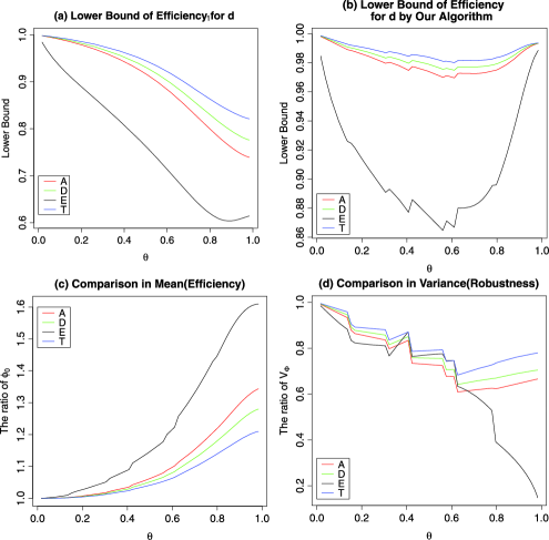
Figure 1: The letters $A$, $D$, $E$ and $T$ represent the choice of criteria function $\Phi$. (a) The lower bound of efficiency $\ell(d_{1})$ for $a=(0,0,\theta,1-\theta)$ with $\theta\in(0,1)$. (b) The lower bound of efficiency $\ell(d)$ with $d$ obtained by algorithm (42). Particularly $\theta=1/2$ implies $d=d_{2}$. (c) The ratio of mean: $\phi_{0}(d)/\phi_{0}(d_{1})$. (d) The ratio of variance: $V_{\Phi}(d)/V_{\Phi}(d_{1})$.

When $p=t=4$ and $n=16$, they proposed a design as shown by Figure 1(b) therein, which is said to be $d_{1}$ here. By algorithm (42), the dropout mechanism $\vec{a}=(0,0,1/2,1/2)$ yields $d_{2}$.

$$d_{2}\dvtx\qquad\begin{array}[]{cccccccccccccccc}2&1&2&3&3&4&3&2&1&1&1&2&4&4&4&3\\ 4&4&3&4&1&1&2&1&2&2&3&4&3&3&2&1\\ 3&2&1&1&2&3&4&4&3&3&4&1&2&2&1&4\\ 3&2&1&1&2&3&4&4&4&4&2&3&1&1&3&2\end{array}.$$

Table 1: Performance of $d_{1}$ under $\vec{a}=(0,0,1/2,1/2)$

$\bolds{\Phi}$	$\bolds{\phi_{0}(d_{1})}$	$\bolds{V_{\Phi}(d_{1})}$	$\bolds{\tilde{e}_{1}(d_{1})}$	$\bolds{g(d_{1})}$	$\bolds{\ell(d_{1})}$
$A$	0.6646345	0.07223834	0.9558432	0.9592851	0.9169261
$D$	0.6747419	0.06776632	0.9603310	0.9693223	0.9308702
$E$	0.5528575	0.09039916	0.8960473	0.8512042	0.7627192
$T$	0.6848634	0.06334558	0.9650531	0.9790485	0.9448338

Table 2: Performance of $d_{2}$ under $\vec{a}=(0,0,1/2,1/2)$

$\bolds{\Phi}$	$\bolds{\phi_{0}(d_{2})}$	$\bolds{V_{\Phi}(d_{2})}$	$\bolds{\tilde{e}_{1}(d_{2})}$	$\bolds{g(d_{2})}$	$\bolds{\ell(d_{2})}$
$A$	0.7058735	0.05266523	0.9989759	0.9748175	0.9738192
$D$	0.7094851	0.05129209	0.9991830	0.9796020	0.9788017
$E$	0.6337475	0.06979073	0.9848636	0.8877519	0.8743145
$T$	0.7130567	0.05005383	0.9993922	0.9843273	0.9837291

Tables 1 and 2 summarize the performances of designs $d_{1}$ and $d_{2}$ under criteria of $A$, $D$, $E$ and $T$. Since $e_{0}(d)\geq\ell(d)=\tilde{e}_{1}(d)g(d)$, a design $d$ would be $\phi_{0}$-efficient if both $\tilde{e}_{1}(d)$ and $g(d)$ are close to unity. Algorithm (42) focuses on $e_{1}(d)$ and provides a satisfactory solution in view of the column of $\tilde{e}_{1}$ in Table 2. We observe that the values of $g$ in both of these tables are very close to unity except for $E$-criterion. Notice that the values of gap function $g$ for $T$-criterion are always the largest among all criteria, which is due to the linearity of $T$-criterion.

In comparison, $d_{2}$ is more efficient and robust than $d_{1}$ under all criteria in view of the columns of $\phi_{0}$ and $V_{\Phi}$, respectively. A lesson from the latter is that a design with a more diverse composition of sequences is generally more robust. Here in $d_{2}$, only the sequences of $1234$ and $4321$ appear twice while each of the remaining sequences appears only once. Low, Lewis and Prescott (1999) had similar observations.

We now consider the performance of a design obtained by algorithm (42) for dropout mechanisms of the form $\vec{a}=(0,0,\theta,1-\theta)$, $0<\theta<1$. By heuristic arguments in Section 2.2, the value of gap function $g$ would be smaller if there is larger variability in $l$. This is supported by the $U$-shape curve of $\ell(d)$ in Figure 1(b). From Figure 1(a), we see that the efficiency of $d_{1}$ has a reverse relationship with the value of $\theta$. Figure 1(c) shows that the advantage of our algorithm against $d_{1}$ is more obvious when there is large chance of dropout. This means that our algorithm succeeded in adapting the choice of designs to different dropout mechanisms. Figure 1(d) shows that the design by our algorithm is also more robust than $d_{1}$ against the randomness of subject dropout. When $p=t=4$ and $n=24$, Low, Lewis and Prescott (1999) proposed a design which consists of two copies of three distinct $4\times 4$ Latin squares, which is denoted by $d_{3}$ here. When $\vec{a}=(0,1/10,2/5,1/2)$ our algorithm yields $d_{4}$ which consists of one copy of the first twelve sequences and two copies of the last six sequences of (48). According to the last two columns of Table 3, $d_{4}$ outperforms $d_{3}$ in terms of both efficiency and robustness with the exception for the robustness under $E$-criterion.

$$d_{4}\dvtx\qquad\begin{array}[]{cccccccccccc@{\hspace*{4pt}}|@{\hspace*{4pt}}cccccc}2&2&2&3&4&4&2&3&3&4&4&3\hfil\hskip 4.0pt\vrule\hskip 4.0&3&4&2&1&1&1\\ 3&4&3&4&3&2&3&4&4&2&2&2\hfil\hskip 4.0pt\vrule\hskip 4.0&1&1&1&2&4&3\\ 4&3&1&1&2&1&1&1&2&1&3&4\hfil\hskip 4.0pt\vrule\hskip 4.0&2&3&4&4&3&2\\ 4&3&1&1&2&1&4&2&1&3&1&1\hfil\hskip 4.0pt\vrule\hskip 4.0&2&3&4&3&2&4\end{array}\times 2.$$ (48)

Table 3: Performance of $d_{3}$ and $d_{4}$ under $\vec{a}=(0,1/10,2/5,1/2)$

$\bolds{\Phi}$	$\bolds{\phi_{0}(d_{4})}$	$\bolds{V_{\Phi}(d_{4})}$	$\bolds{\tilde{e}_{1}(d_{4})}$	$\bolds{g(d_{4})}$	$\bolds{\ell(d_{4})}$	$\bolds{\phi_{0}(d_{4},d_{3})}$	$\bolds{V_{\Phi}(d_{4},d_{3})}$
$A$	0.6791	0.0526	0.999983	0.9777	0.9777	1.0112	0.9705
$D$	0.6822	0.0516	0.999983	0.9822	0.9821	1.0115	0.9631
$E$	0.6118	0.0648	0.999979	0.8809	0.8809	1.0089	1.0386
$T$	0.6852	0.0506	0.999983	0.9866	0.9869	1.0118	0.9562

5.1.2 Comparison to designs of Bose and Bagchi (2008), Majumdar, Dean and Lewis (2008) and Zhao and Majumdar (2012)

When the realization of subject dropout $l$ is not random, we have $\phi_{0}\equiv\phi_{1}$. In this case, Bose and Bagchi (2008) have the following results: [(1)]

When $p=t\geq 3$ is a prime or primer power and $n=t(t-1)$, a design is found to be universally optimal whenever $a_{q}=1$ for any $3\leq q\leq p$.

When $p=t\geq 3$ is a prime or primer power, $t\equiv 3$(mod $4$) and $n=2t$, a design is found to be universally optimal whenever $a_{q}=1$ with $q=(p+1)/2$ or $p$.

When $p=t\geq 3$ is a prime or primer power, $t\equiv 1$(mod $4$) and $n=4t$, a design is found to be universally optimal whenever $a_{q}=1$ with $q=(p+1)/2$ or $p$.

For example, when $t=p=5$ the smallest $n$ should be $4t=20$. In this case the design proposed by them is universally optimal, either when the experiment is complete or when all subjects immediately drop out after period $3$ with probability $1$, that is, $a_{3}=1$. We denote this design by $d_{5}$ which is given by Example 3 of Bose and Bagchi (2008). When $\vec{a}=(0,1/20,3/20,1/5,3/5)$ algorithm (42) yields $d_{6}$ as follows:

$$d_{6}\dvtx\qquad\begin{array}[]{cccccccccccccccccccc}1&2&4&4&3&2&1&2&1&1&3&2&4&5&5&5&5&3&4&3\\ 2&5&1&2&1&3&2&3&5&4&4&5&5&4&4&2&3&1&3&1\\ 3&4&3&5&5&4&4&5&3&3&1&1&1&2&2&1&2&2&5&4\\ 4&1&5&3&2&5&3&1&2&2&5&3&3&1&1&4&4&4&2&5\\ 4&1&5&3&2&1&5&4&4&5&2&4&2&3&3&3&1&5&1&2\end{array}.$$

Table 4 shows that $d_{6}$ is more efficient and robust than $d_{5}$ under criteria of $A$, $D$ and $T$, while the result is reversed under the criterion of $E$. The reason for the latter is that $d_{5}$ did a better job in avoiding disconnected designs under subject dropout, that is, $\Phi_{E}(C_{d}(\tau,l))=0$.

Table 4: Performance of $d_{5}$ and $d_{6}$ under $\vec{a}=(0,1/20,3/20,1/5,3/5)$

$\bolds{\Phi}$	$\bolds{\phi_{0}(d_{6})}$	$\bolds{V_{\Phi}(d_{6})}$	$\bolds{\tilde{e}_{1}(d_{6})}$	$\bolds{g(d_{6})}$	$\bolds{\ell(d_{6})}$	$\bolds{\phi_{0}(d_{6},d_{5})}$	$\bolds{V_{\Phi}(d_{6},d_{5})}$
$A$	0.7555	0.05944	0.99888	0.97848	0.97738	1.00117	0.98842
$D$	0.7589	0.05827	0.99891	0.98277	0.98170	1.00172	0.98333
$E$	0.6712	0.07399	0.99091	0.87621	0.86825	0.99449	1.03435
$T$	0.7621	0.05719	0.99894	0.98700	0.98595	1.00224	0.97877

Table 5: Performance of $d_{7}$ and $d_{8}$ under $\vec{a}=(0,0,1/3,1/3,1/3)$

$\bolds{\Phi}$	$\bolds{\phi_{0}(d_{8})}$	$\bolds{V_{\Phi}(d_{8})}$	$\bolds{\tilde{e}_{1}(d_{8})}$	$\bolds{g(d_{8})}$	$\bolds{\ell(d_{8})}$	$\bolds{\phi_{0}(d_{8},d_{7})}$	$\bolds{V_{\Phi}(d_{8},d_{7})}$
$A$	1.2340	0.053908	1	0.99591	0.99591	1.11018	0.57705
$D$	1.2347	0.053736	1	0.99643	0.99643	1.10598	0.59362
$E$	1.2004	0.059782	1	0.96877	0.96877	1.16339	0.51397
$T$	1.2353	0.053573	1	0.99696	0.99696	1.10177	0.60992

Since the magnitude of the differences between $d_{5}$ and $d_{6}$ are small in terms of both efficiency and robustness, we conclude that the designs of Bose and Bagchi (2008) successfully defended the loss of information due to subject dropout. The same conclusion applies to Majumdar, Dean and Lewis (2008) and Zhao and Majumdar (2012) since they use similar ideas.

5.1.3 Comparisons to designs of Kushner (1998)

Kushner (1998) derived conditions for universal optimality as a special case of ours under complete experiment. Particularly, when $t=3$, $p=5$ and $n=30$, Example 4 of Kushner (1998) gives a design satisfying the optimality equations therein, which is denoted $d_{7}$ here. When $\vec{a}=(0,0,1/3,1/3,1/3)$ our algorithm gives $d_{8}$ which consist of five copies of (55),

$$d_{8}\dvtx\qquad\begin{array}[]{cccccc}1&2&3&3&1&2\\ 3&3&2&1&2&1\\ 2&1&1&2&3&3\\ 2&1&1&2&3&3\\ 1&2&3&3&2&1\end{array}\times 5.$$ (55)

Based on Table 5 $d_{8}$ outperforms $d_{7}$ in terms of both efficiency and robustness even though $d_{7}$ is universally optimal under complete experiment.

5.2 Symmetric exact designs

This section illustrates the usage of Theorem 5 in deriving efficient symmetric exact designs. By Remark 4 in Section 3.5, when $t=2$, $p=6$ and $m=p-1=5$, inequality (20) in Theorem 3 always holds regardless of the value of $\vec{a}$. By applying Theorem 3(i), we have $x^{*}=0$ and hence $q_{s}^{\prime}(x^{*})=2q_{s12}$. Moreover, it is easy to see that the support ${\mathcal{T}}$ essentially contains all sequences which assign a subject to each of the two treatments for $3$ out of the total of $6$ periods, and hence $|{\mathcal{T}}|=20$. Within each symmetric block, there are two sequences since $t=2$. Hence there are $10$ symmetric blocks. However, it is not necessary to include all these symmetric blocks in the design. Particularly when $\vec{a}=(0,0,0,0,2/5,3/5)$, we have $q_{s_{1}}^{\prime}(x^{*})/q_{s_{2}}^{\prime}(x^{*})=q_{s_{1}12}/q_{s_{2}12}=-6.01$ for $s_{1}=122121$ and $s_{2}=122211$. In the spirit of Theorem 5 we propose a small sized design, $d_{9}$, which consists of one copy of sequences $122121$ and $211212$ and six copies of the sequences $122211$ and $211122$. So we have $n=14$ for $d_{9}$. The point is that we have the freedom of selecting different subclasses of ${\mathcal{T}}$. The performance of $d_{9}$ is given in Table 6. It shows the high efficiency and robustness of $d_{9}$. Note that when $t=2$ all criteria are equivalent.

Table 6: Performance of $d_{9}$ under $\vec{a}=(0,0,0,0,2/5,3/5)$

$\bolds{\Phi}$	$\bolds{\phi_{0}(d_{9})}$	$\bolds{V_{\Phi}(d_{9})}$	$\bolds{\tilde{e}_{1}(d_{9})}$	$\bolds{g(d_{9})}$	$\bolds{\ell(d_{9})}$
$A$, $D$, $E$, $T$ and etc.	2.7368	0.09152	0.99511	0.997823	0.99295

6 Discussions

Subject dropout is a very important issue in planning a crossover design. It is shown by Table 5 and other examples in literature that an optimal design under complete experiment is no longer optimal and possibly even disconnected when there is subject dropout. However, the problem has received very limited attention in literature so far, and the majority of the research assumes that there is no subject dropout. Bose and Bagchi (2008), Majumdar, Dean and Lewis (2008), Zhao and Majumdar (2012) all considered the nested structure such that a design, together with its subdesign, obtained by taking only the first $q$($<p$) periods, are both optimal or efficient. Naturally such designs would still be efficient when all subjects drop out at periods between $p$ and $q$. The issue with this approach is that we lose adaptation to different dropout mechanisms. Furthermore, their methods only apply to special configurations of $p,t,n$.

In order to take into account the dropout mechanism, one has to make assumptions to formulate the dropout mechanism. This paper adopts two mild assumptions and works on the target function $\phi_{0}$ which is given by taking the expectation of a regular optimality criterion with respect to a given dropout mechanism. Actually Low, Lewis and Prescott (1999) have followed the same approach. However, they only provided two case studies, and there were no theoretical results regarding how to identify an efficient design in general. The latter problem is itself intractable. To tackle it, we propose to use the surrogate target function of $\phi_{1}$ in place of $\phi_{0}$. It turns out that this replacement is very successful. Examples in Section 5 show that $\phi_{1}$-optimal (or highly efficient) designs are also highly efficient under $\phi_{0}$. Moreover, these designs are also shown to be very robust against the randomness of subject dropout due to the substantial diversity in the composition of treatment sequences.

Theoretically, we derive feasible, equivalent conditions for a design to be $\phi_{1}$-universally optimal in asymptotic design theory. These conditions are essentially linear equations with respect to proportions of treatment sequences from ${\mathcal{T}}$, a subclass of all possible treatment sequences. A solution for the equations, which yields an exact design, does not necessarily exist due to the discrete nature of the problem. However, one can follow the spirit of the conditions and easily propose an applicable algorithm to derive an efficient exact design for any criterion and any configuration of $p,t,n$. In this paper, we adopt algorithm (42) for general designs as well as the approach in Section 5.2 for symmetric designs.

The problem of identifying exact designs for large values of $p$ and $t$ remains as an open problem. The critical difficulty is that as $p$ and $t$ grow the size of the support for admissible sequences, $|{\mathcal{T}}|$, increases very fast. Typically ${\mathcal{T}}$ contains two distinct symmetric blocks, in which case $p=t=6$ usually yields $|{\mathcal{T}}|=2\times 6!=1440$. That means the majority of the sequences in ${\mathcal{T}}$ would not appear in the design for a moderate value of $n$. The same issue has appeared in Kushner (1997b). If we adopt the approach of symmetric designs as in Section 5.2 we would need $n$ to be as of the same magnitude as $|{\mathcal{T}}|$. On the other hand, algorithm (42) is essentially an integer programming problem and the number of the integer variables is equal to $|{\mathcal{T}}|$. Hence it would be infeasible for a computer to handle when $|{\mathcal{T}}|$ is too large. For this problem, one possible solution is to reduce the size of ${\mathcal{T}}$ through the study of intrinsic relationships among treatment sequences. Another approach is to resort to algorithm improvement.

7 Proofs

Proof of Lemma 3 It would be enough to show that $V={\mathbb{E}}O$. First, it is easy to show that $B^{m_{1}}_{ij}B^{m_{2}}_{jk}=B^{\mathrm{min}(m_{1},m_{2})}_{ik}$. We have $MU=\operatorname{diag}(1_{l_{1}},1_{l_{2}},\ldots,\break 1_{l_{n}})$ and $MZ=({I_{l_{1}p}^{l_{1}{}^{\prime}}},{I_{l_{2}p}^{l_{2}{}^{\prime}}},\ldots,{I_{l_{n}p}^{l_{n}{}^{\prime}}})^{\prime}$. Then we have

$$\operatorname{pr}^{\perp}(MU) = \operatorname{diag}(B_{l_{1}},\ldots,B_{l_{n}}),$$

$$\operatorname{pr}^{\perp}(MU)MZ = \bigl{(}{B_{l_{1}p}^{l_{1}{}^{\prime}}},{B_{l_{2}p}^{l_{2}{}^{\prime}}},\ldots,{B_{l_{n}p}^{l_{n}{}^{\prime}}}\bigr{)}^{\prime},$$

$$Z^{\prime}M^{\prime}\operatorname{pr}^{\perp}(MU)MZ = \sum^{n}_{u=1}B_{p}^{l_{u}}=\sum^{p}_{i=1}h_{i}B_{p}^{i}.$$

Without loss of generality, we could assume $h_{p}>0$. Then one choice of the $g$-inverse of $Z^{\prime}M^{\prime}\operatorname{pr}^{\perp}(MU)MZ$ is $\sum^{p}_{i=1}g_{i}B_{p}^{i}$ where

$$g_{i} = r_{i}^{-1}-r_{i+1}^{-1},\qquad 1\leq i\leq p-1,$$ (56)

$$g_{p} = h_{p}^{-1},$$ (57)

with $h_{k}=\sum^{n}_{i=1}1_{l_{i}=k},1\leq k\leq p$, and $r_{i}=\sum^{p}_{k=i}h_{i}$ denotes the number of subjects remaining at period $i$, $1\leq i\leq p$. Note that if $h_{p}=0$, the value of $p$ in (56) and (57) should be replaced by $\tilde{p}=\operatorname{max}\{k\dvtx h_{k}>0\}$, and for $k>\tilde{p}$ we let $h_{k}=0$. It is easily seen that the following arguments and thus the lemma would still hold. Now we have

$$\operatorname{pr}^{\perp}(MZ|MU) = \operatorname{pr}^{\perp}(MU)-\operatorname{pr}\bigl{(}\operatorname{pr}^{\perp}(MU)MZ\bigr{)}$$

$$= \operatorname{diag}(B_{l_{1}},\ldots,B_{l_{n}})-\Delta,$$

$$\Delta = \Biggl{(}\sum^{p}_{k=1}g_{k}B_{l_{i}l_{j}}^{\min(k,l_{i},l_{j})}\Biggr{)}_{i,j=1,2,\ldots,n}.$$

Let $O=(O_{ij})_{1\leq i,j\leq n}=M^{\prime}\operatorname{pr}^{\perp}(MZ|MU)M$, and then we have

$$O_{ii} = B_{p}^{l_{i}}-\sum^{p}_{k=1}g_{k}B_{p}^{\mathrm{min}(k,l_{i})},$$

$$O_{ij} = -\sum^{p}_{k=1}g_{k}B_{p}^{\mathrm{min}(k,l_{i},l_{j})}.$$

We will derive the expectation of $\sum^{p}_{k=1}g_{k}B_{p}^{\mathrm{min}(k,l_{i})}$ and other components could be dealt with by similar arguments. First we have the decomposition

$$\sum^{p}_{k=1}g_{k}B_{p}^{\mathrm{min}(k,l_{i})} = \sum^{l_{i}-1}_{k=1}g_{k}B_{p}^{k}+\sum^{p}_{k=l_{i}}g_{k}B_{p}^{l_{i}}$$

$$= \sum^{l_{i}-1}_{k=1}\biggl{(}\frac{1}{r_{k}}-\frac{1}{r_{k+1}}\biggr{)}B_{p}^{k}+\frac{1}{r_{l_{i}}}B_{p}^{l_{i}}.$$

When $k\leq l_{i}$ and $l_{i}$ is given, we know that $r_{k}-1$ follows the binomial distribution with parameters $n-1$ and $a_{kp}$. Hence we have

$${\mathbb{E}}\bigl{(}r_{k}^{-1}|l_{i},k\leq l_{i}\bigr{)} = \sum^{n-1}_{j=0}\frac{1}{j+1}\frac{(n-1)!}{(n-1-j)!j!}a_{kp}^{j}(1-a_{kp})^{n-1-j}$$

$$= \frac{1-(1-a_{kp})^{n}}{na_{kp}}:=b_{k}.$$

Hence we have

$${\mathbb{E}}\Biggl{(}\sum^{p}_{k=1}g_{k}B_{p}^{\mathrm{min}(k,l_{i})}\bigg{|}l_{i},1\leq i\leq n\Biggr{)} = \sum^{l_{i}-1}_{k=1}(b_{k}-b_{k+1})B_{p}^{k}+b_{l_{i}}B_{p}^{l_{i}}$$

$$= \sum^{p}_{k=1}\bigl{[}(b_{k}-b_{k+1})1_{[k<l_{i}]}+b_{k}1_{[k=l_{i}]}\bigr{]}B_{p}^{k}.$$

Here we have the convention of $b_{p+1}=0$ for notational convenience. Hence

$${\mathbb{E}}\Biggl{(}\sum^{p}_{k=1}g_{k}B_{p}^{\mathrm{min}(k,l_{i})}\Biggr{)} = \sum^{p}_{k=1}\bigl{[}(b_{k}-b_{k+1})a_{k+1,p}+b_{k}(a_{kp}-a_{k+1,p})\bigr{]}B_{p}^{k}$$

$$= \sum^{p}_{k=1}(a_{kp}b_{k}-a_{k+1,p}b_{k+1})B_{p}^{k}$$

$$= \frac{1}{n}\sum^{p}_{k=1}\bigl{(}a_{1k}^{n}-a_{1,k-1}^{n}\bigr{)}B_{p}^{k}.$$

Following this strategy, it is easy to show that

$${\mathbb{E}}O_{ii} = \sum^{p}_{k=1}\bigl{[}a_{k}-n^{-1}\bigl{(}a_{1k}^{n}-a_{1,k-1}^{n}\bigr{)}\bigr{]}B_{p}^{k},$$

$${\mathbb{E}}O_{ij} = -\frac{1}{n}\sum^{p}_{k=1}\bigl{(}a_{k}+a_{k+1,p}a_{1k}^{n}-a_{kp}a_{1,k-1}^{n}\bigr{)}B_{p}^{k}.$$

Then we have $V={\mathbb{E}}O$.

Proof of Theorem 2 By definition of symmetric designs we have

$$T_{\sigma d} = T_{d}S_{\sigma}$$ (58)

$$= (\tilde{S}_{\sigma,d}\otimes I_{p})T_{d},$$

$$F_{\sigma d} = (\tilde{S}_{\sigma,d}\otimes I_{p})F_{d},$$

where $\tilde{S}_{\sigma,d}$ is a permutation matrix for subjects induced by $\sigma$ and (symmetric) $d$. Note that we have $(\tilde{S}_{\sigma,d}\otimes I_{p})^{\prime}V(\tilde{S}_{\sigma,d}\otimes I_{p})=V$. So $C_{dij},1\leq i,j\leq 2$, are completely symmetric and hence $C_{d}$ is completely symmetric for a symmetric design $d$. This yields

$$C_{d}=\overline{C}_{d},$$

and the equality in (10). By (58) we have $\overline{T}=\overline{T}S_{\sigma}$ for any $\sigma\in{\mathcal{B}}$ and hence $\overline{T}=n^{-1}1_{p}1_{t}^{\prime}$. Hence we have $\hat{\overline{T}}=\overline{T}B_{t}=0$. By the same argument we have $\hat{\overline{F}}=0$. Then the equality in (3.2) holds, and so does the equality in (13). Hence we proved $\operatorname{tr}(C_{d})=q_{d}^{*}$.

Given any design $d$ with corresponding $P=(p_{s},s\in{\mathcal{S}})$, we could define a new design $\bar{d}\leftrightarrow P_{\bar{d}}=(\bar{p}_{s},s\in{\mathcal{S}})$ by

$$P_{\bar{d}}=\frac{\sum_{\sigma\in{\mathcal{P}}}P_{\sigma d}}{t!}.$$ (59)

Then we have $\sum_{s\in{\mathcal{S}}}p_{s}q_{s}(x)=\sum_{s\in{\mathcal{S}}}\bar{p}_{s}q_{s}(x)$ in view of (36) and $q_{d}^{*}=q^{*}_{\bar{d}}$.

Proof of Theorem 3 In the following, we would apply Lemma 3.1 of Kushner (1997a) to prove (iii). The proof of (i) and (ii) follows from similar arguments. Given any sequence $s$, we have $q_{s}(x)=\sum^{p}_{k=m}\alpha_{k}q_{s}^{k}(x)$ where $q_{s}^{k}(x)=q_{s11}^{k}+2q_{s12}^{k}x+q_{s22}^{k}x^{2}$ and $q_{sij}^{k}=\operatorname{tr}(G_{i}^{\prime}B^{k}_{p}G_{j})$ with $G_{1}=\hat{T}_{u}$ and $G_{2}=\hat{F}_{u}$. By direct calculation we have

$$q_{s11}^{k} = k-\xi_{s_{k}}/k,$$

$$q_{s12}^{k} = (k\rho_{s_{k}}+f_{s_{k},t_{k}}-\xi_{s_{k}})/k,$$

$$q_{s22}^{k} = (kt-1)(k-1)/kt-(\xi_{s_{k}}-2f_{{s_{k}},t_{k}}+1)/k,$$

where $\xi_{s_{k}}=\sum^{t}_{i=1}(f_{s_{k},i})^{2}$ and $\rho_{s_{k}}=\sum^{k-1}_{j=1}1_{t_{j}=t_{j+1}}$. For notational simplicity we define $\xi_{k}=\xi_{s_{k}}$, $\rho_{k}=\rho_{s_{k}}$ and $f_{k}=f_{s_{k},t_{k}}$. Also let $\Xi_{A},A\subset\{x,k,p,t\}$, denote a quantity that depends on the elements of $A$, and $a\propto_{k}b$ means that $a/b$ is a quantity that only depend on $k$. Then

$$q_{s}^{k}(x) \propto_{k} -\xi_{k}(x+1)^{2}+2f_{k}\bigl{(}x+x^{2}\bigr{)}+2k\rho_{k}x+\Xi_{k,t,x}$$ (61)

$$= -(\xi_{k}-2f_{k})(x+1)^{2}+2k(\rho_{k}-f_{k})x$$

$${}+2f_{k}\bigl{[}(k-1)x-1\bigr{]}+\Xi_{k,t,x}.$$

From (61), for any $x>0$, the sequence which maximizes $q_{s}^{k}(x)$ has to be of the form $(1*1_{f_{s_{k},1}}|2*1_{f_{s_{k},2}}|\ldots\ldots|(t-1)*1_{f_{s_{k},t-1}}|t*1_{f_{s_{k},t}})$ with the restrictions of $f_{s_{k},i+1}\geq f_{s_{k},i},i=1,2,\ldots,t-1$ and $f_{s_{k},t-1}-f_{s_{k},1}\leq 1$. For the special case of $k\leq t$, the sequence reduces to the form of $(1,2,\ldots,k-h,t*1_{h}).$ By (61) the sequence of $\langle re\rangle$ maximizes $q_{s}(x)$ for any $x\in((p-1)^{-1},(p-2)^{-1}]$ since this sequence maximizes $q_{s}^{k}(x)$ for all $k=m,\ldots,p$. Since all the sequences in the class of $\langle re\rangle$ have the same value of $d(q_{s}(x))/dx$, we need to choose $x$ so that the derivative is zero, and hence (iii) is proven.

Proof of Theorem 4 By Lemma 4, equations (31)–(35) is equivalent to

$$\check{C}_{d11}+x^{*}\check{C}_{d12}B_{t} = \frac{ny^{*}}{t-1}B_{t},$$ (62)

$$\check{C}_{d21}+x^{*}\check{C}_{d22}B_{t} = 0,$$ (63)

$$B\bigl{(}\hat{\overline{T}}+x^{*}\hat{\overline{F}}\bigr{)} = 0.$$ (64)

First we show the necessity. Let $f$ be a symmetric optimal design and $g$ be a new design with $P_{g}=P_{d}/2+P_{f}/2$. Then by Lemmas 1 and 5 wehave

$$\check{C}_{g} \geq \check{C}_{d}/2+\check{C}_{f}/2$$

$$= \frac{ny^{*}}{t-1}B_{t}.$$

Let $\bar{g}$ be the symmetrized version of design $g$ as defined by (59). Following the same argument as in Lemma 1 we have

$$\sum_{\sigma\in{\mathcal{P}}}S_{\sigma}^{\prime}\check{C}_{g}S_{\sigma}/|{\mathcal{P}}|\leq C_{\bar{g}}.$$ (66)

Combining (7) and (66) we have

$$C_{\bar{g}}=\frac{ny^{*}}{t-1}B_{t},$$

in view of Corollary 2(ii). Then we have $\operatorname{tr}(\check{C}_{d})=ny^{*}$ which together with (7) yields

$$\check{C}_{g}=\frac{ny^{*}}{t-1}B_{t}.$$

Following similar arguments as in Theorem 5.3 of Kushner (1997b) we have

$$\check{C}_{f22}\check{C}_{g22}^{+}\check{C}_{g21} = \check{C}_{f21},$$ (67)

$$\check{C}_{d22}\check{C}_{g22}^{+}\check{C}_{g21} = \check{C}_{d21},$$ (68)

where $G^{+}$ denotes the Moore–Penrose inverse of $G$. Since $f$ is a symmetric design, we have $\check{C}_{f21}=q_{f12}B_{t}/(t-1)$ and $\check{C}_{f22}=q_{f22}B_{t}/(t-1)+(1_{t}^{\prime}\check{C}_{f22}1_{t})J_{t}/t^{2}$. So we have $\check{C}_{f22}^{+}=(t-1)B_{t}/q_{f22}+J_{t}/(1_{t}^{\prime}\check{C}_{f22}1_{t})$. By left multiplying both sides of (67) we have

$$\check{C}_{g22}^{+}\check{C}_{g21} = \check{C}_{f22}^{+}\check{C}_{f21}$$

$$= -x^{*}B_{t}.$$

By plugging (7) into (68) we have (63). Then we have

$$\frac{ny^{*}}{t-1}B_{t}=\check{C}_{d} = \check{C}_{d11}-\check{C}_{d12}\check{C}_{d22}^{-}\check{C}_{d21}$$

$$= \check{C}_{d11}+x^{*}\check{C}_{d12}\check{C}_{d22}^{-}\check{C}_{d22}B_{t}$$

$$= \check{C}_{d11}+x^{*}\check{C}_{d12}B_{t}.$$

Hence (62) is derived. From (10) and (5.3) of Kushner (1997b) we have

$$ny^{*} = \operatorname{tr}(\overline{C}_{d})$$

$$\leq \operatorname{tr}(\tilde{C}_{d})$$

$$\leq \operatorname{tr}\bigl{(}\overline{C}_{d11}+2x\overline{C}_{d12}+x^{2}\overline{C}_{d22}\bigr{)}$$

$$= q_{d}(x)-n\operatorname{tr}\bigl{[}(\hat{\overline{T}}_{d}+x\hat{\overline{F}}_{d})^{\prime}B(\hat{\overline{T}}_{d}+x\hat{\overline{F}}_{d})\bigr{]}.$$

Setting $x=x^{*}$ in (7) gives $y^{*}\leq y^{*}-\operatorname{tr}[(\hat{\overline{T}}_{d}+x^{*}\hat{\overline{F}}_{d})^{\prime}B(\hat{\overline{T}}_{d}+x^{*}\hat{\overline{F}}_{d})]$ which yields (64) due to Pukelsheim [(1993), page 15].

Now we show the sufficiency. By utilizing (62), (63) and (64) we have

$$C_{d11}+x^{*}C_{d12}B_{t} = \frac{ny^{*}}{t-1}B_{t},$$

$$C_{d21}+x^{*}C_{d22}B_{t} = 0,$$

which in turn yields

$$C_{d} = C_{11}+x^{*}C_{d12}C_{d22}^{-}C_{d22}B_{t}$$

$$= \frac{ny^{*}}{t-1}B_{t}.$$

References

• Bose and Bagchi (2008) {barticle}[mr] \bauthor\bsnmBose, \bfnmMausumi\binitsM. and \bauthor\bsnmBagchi, \bfnmSunanda\binitsS. (\byear2008). \btitleOptimal crossover designs under premature stopping. \bjournalUtil. Math. \bvolume75 \bpages273–285. \bidissn=0315-3681, mr=2392763 \bptokimsref \endbibitem
• Bose and Dey (2009) {bbook}[mr] \bauthor\bsnmBose, \bfnmMausumi\binitsM. and \bauthor\bsnmDey, \bfnmAloke\binitsA. (\byear2009). \btitleOptimal Crossover Designs. \bpublisherWorld Scientific, \blocationHackensack, NJ. \biddoi=10.1142/9789812818430, mr=2524180 \bptokimsref \endbibitem
• Chêng and Wu (1980) {barticle}[mr] \bauthor\bsnmChêng, \bfnmCh’ing Shui\binitsC. S. and \bauthor\bsnmWu, \bfnmChien-Fu\binitsC.-F. (\byear1980). \btitleBalanced repeated measurements designs. \bjournalAnn. Statist. \bvolume8 \bpages1272–1283. \bidissn=0090-5364, mr=0594644 \bptokimsref \endbibitem
• Godolphin (2004) {barticle}[mr] \bauthor\bsnmGodolphin, \bfnmJ. D.\binitsJ. D. (\byear2004). \btitleSimple pilot procedures for the avoidance of disconnected experimental designs. \bjournalJ. Roy. Statist. Soc. Ser. C \bvolume53 \bpages133–147. \biddoi=10.1046/j.0035-9254.2003.05054.x, issn=0035-9254, mr=2043764 \bptokimsref \endbibitem
• Hedayat and Afsarinejad (1978) {barticle}[mr] \bauthor\bsnmHedayat, \bfnmA.\binitsA. and \bauthor\bsnmAfsarinejad, \bfnmK.\binitsK. (\byear1978). \btitleRepeated measurements designs. II. \bjournalAnn. Statist. \bvolume6 \bpages619–628. \bidissn=0090-5364, mr=0488527 \bptokimsref \endbibitem
• Hedayat and Yang (2003) {barticle}[mr] \bauthor\bsnmHedayat, \bfnmA. S.\binitsA. S. and \bauthor\bsnmYang, \bfnmMin\binitsM. (\byear2003). \btitleUniversal optimality of balanced uniform crossover designs. \bjournalAnn. Statist. \bvolume31 \bpages978–983. \biddoi=10.1214/aos/1056562469, issn=0090-5364, mr=1994737 \bptokimsref \endbibitem
• Hedayat and Yang (2004) {barticle}[mr] \bauthor\bsnmHedayat, \bfnmA. S.\binitsA. S. and \bauthor\bsnmYang, \bfnmMin\binitsM. (\byear2004). \btitleUniversal optimality for selected crossover designs. \bjournalJ. Amer. Statist. Assoc. \bvolume99 \bpages461–466. \biddoi=10.1198/016214504000000331, issn=0162-1459, mr=2062831 \bptokimsref \endbibitem
• Hedayat and Zheng (2010) {barticle}[mr] \bauthor\bsnmHedayat, \bfnmA. S.\binitsA. S. and \bauthor\bsnmZheng, \bfnmWei\binitsW. (\byear2010). \btitleOptimal and efficient crossover designs for test-control study when subject effects are random. \bjournalJ. Amer. Statist. Assoc. \bvolume105 \bpages1581–1592. \biddoi=10.1198/jasa.2010.tm10134, issn=0162-1459, mr=2796573 \bptokimsref \endbibitem
• Huynh and Feldt (1970) {barticle}[auto:STB—2013/01/23—16:20:06] \bauthor\bsnmHuynh, \bfnmH.\binitsH. and \bauthor\bsnmFeldt, \bfnmL. S.\binitsL. S. (\byear1970). \btitleConditions under which mean square ratios in repeated measurements designs have exact $F$-distributions. \bjournalJ. Amer. Statist. Assoc. \bvolume65 \bpages1582–1589. \bptokimsref \endbibitem
• Jones and Kenward (2003) {bbook}[mr] \bauthor\bsnmJones, \bfnmByron\binitsB. and \bauthor\bsnmKenward, \bfnmMichael G.\binitsM. G. (\byear2003). \btitleDesign and Analysis of Cross-Over Trials, \bedition2nd ed. \bpublisherChapman & Hall, \blocationLondon. \bptokimsref \endbibitem
• Kiefer (1975) {bincollection}[mr] \bauthor\bsnmKiefer, \bfnmJ.\binitsJ. (\byear1975). \btitleConstruction and optimality of generalized Youden designs. In \bbooktitleA Survey of Statistical Design and Linear Models (Proc. Internat. Sympos., Colorado State Univ., Ft. Collins, Colo., 1973) (\beditor\binitsJ. N.\bfnmJ. N. \bsnmSrivastava, ed.) \bpages333–353. \bpublisherNorth-Holland, \blocationAmsterdam. \bidmr=0395079 \bptokimsref \endbibitem
• Kunert (1984) {barticle}[mr] \bauthor\bsnmKunert, \bfnmJoachim\binitsJ. (\byear1984). \btitleOptimality of balanced uniform repeated measurements designs. \bjournalAnn. Statist. \bvolume12 \bpages1006–1017. \biddoi=10.1214/aos/1176346717, issn=0090-5364, mr=0751288 \bptokimsref \endbibitem
• Kunert and Martin (2000) {barticle}[mr] \bauthor\bsnmKunert, \bfnmJ.\binitsJ. and \bauthor\bsnmMartin, \bfnmR. J.\binitsR. J. (\byear2000). \btitleOn the determination of optimal designs for an interference model. \bjournalAnn. Statist. \bvolume28 \bpages1728–1742. \biddoi=10.1214/aos/1015957478, issn=0090-5364, mr=1835039 \bptokimsref \endbibitem
• Kunert and Stufken (2002) {barticle}[mr] \bauthor\bsnmKunert, \bfnmJ.\binitsJ. and \bauthor\bsnmStufken, \bfnmJ.\binitsJ. (\byear2002). \btitleOptimal crossover designs in a model with self and mixed carryover effects. \bjournalJ. Amer. Statist. Assoc. \bvolume97 \bpages898–906. \biddoi=10.1198/016214502388618681, issn=0162-1459, mr=1941418 \bptokimsref \endbibitem
• Kushner (1997a) {barticle}[mr] \bauthor\bsnmKushner, \bfnmH. B.\binitsH. B. (\byear1997a). \btitleOptimality and efficiency of two-treatment repeated measurements designs. \bjournalBiometrika \bvolume84 \bpages455–468. \biddoi=10.1093/biomet/84.2.455, issn=0006-3444, mr=1467060 \bptokimsref \endbibitem
• Kushner (1997b) {barticle}[mr] \bauthor\bsnmKushner, \bfnmH. B.\binitsH. B. (\byear1997b). \btitleOptimal repeated measurements designs: The linear optimality equations. \bjournalAnn. Statist. \bvolume25 \bpages2328–2344. \biddoi=10.1214/aos/1030741075, issn=0090-5364, mr=1604457 \bptokimsref \endbibitem
• Kushner (1998) {barticle}[mr] \bauthor\bsnmKushner, \bfnmH. B.\binitsH. B. (\byear1998). \btitleOptimal and efficient repeated-measurements designs for uncorrelated observations. \bjournalJ. Amer. Statist. Assoc. \bvolume93 \bpages1176–1187. \biddoi=10.2307/2669860, issn=0162-1459, mr=1649211 \bptokimsref \endbibitem
• Low, Lewis and Prescott (1999) {barticle}[auto:STB—2013/01/23—16:20:06] \bauthor\bsnmLow, \bfnmJ. L.\binitsJ. L., \bauthor\bsnmLewis, \bfnmS. M.\binitsS. M. and \bauthor\bsnmPrescott, \bfnmP.\binitsP. (\byear1999). \btitleAssessing robustness of crossover designs to subjects dropping out. \bjournalStatist. Comput. \bvolume9 \bpages219–227. \bptokimsref \endbibitem
• Majumdar, Dean and Lewis (2008) {barticle}[mr] \bauthor\bsnmMajumdar, \bfnmDibyen\binitsD., \bauthor\bsnmDean, \bfnmAngela M.\binitsA. M. and \bauthor\bsnmLewis, \bfnmSusan M.\binitsS. M. (\byear2008). \btitleUniformly balanced repeated measurements designs in the presence of subject dropout. \bjournalStatist. Sinica \bvolume18 \bpages235–253. \bidissn=1017-0405, mr=2384987 \bptokimsref \endbibitem
• Matthews (1988) {barticle}[mr] \bauthor\bsnmMatthews, \bfnmJ. N. S.\binitsJ. N. S. (\byear1988). \btitleRecent developments in crossover designs. \bjournalInternat. Statist. Rev. \bvolume56 \bpages117–127. \biddoi=10.2307/1403636, issn=0306-7734, mr=0963525 \bptokimsref \endbibitem
• Pukelsheim (1993) {bbook}[mr] \bauthor\bsnmPukelsheim, \bfnmFriedrich\binitsF. (\byear1993). \btitleOptimal Design of Experiments. \bpublisherWiley, \blocationNew York. \bidmr=1211416 \bptokimsref \endbibitem
• Ratkowsky, Evans and Alldredge (1992) {bbook}[auto:STB—2013/01/23—16:20:06] \bauthor\bsnmRatkowsky, \bfnmD. A.\binitsD. A., \bauthor\bsnmEvans, \bfnmM. A.\binitsM. A. and \bauthor\bsnmAlldredge, \bfnmJ. R.\binitsJ. R. (\byear1992). \btitleCross-Over Experiments: Design, Analysis, and Application. \bpublisherDekker, \blocationNew York. \bptokimsref \endbibitem
• Senn (2003) {bbook}[auto:STB—2013/01/23—16:20:06] \bauthor\bsnmSenn, \bfnmS.\binitsS. (\byear2003). \btitleCross-over Trials in Clinical Research, \bedition2nd ed. \bpublisherWiley, \blocationChichester. \bptokimsref \endbibitem
• Stufken (1991) {barticle}[mr] \bauthor\bsnmStufken, \bfnmJohn\binitsJ. (\byear1991). \btitleSome families of optimal and efficient repeated measurements designs. \bjournalJ. Statist. Plann. Inference \bvolume27 \bpages75–83. \biddoi=10.1016/0378-3758(91)90083-Q, issn=0378-3758, mr=1089354 \bptokimsref \endbibitem
• Stufken (1996) {bincollection}[mr] \bauthor\bsnmStufken, \bfnmJohn\binitsJ. (\byear1996). \btitleOptimal crossover designs. In \bbooktitleDesign and Analysis of Experiments (\beditor\binitsS.\bfnmS. \bsnmGhosh and \beditor\binitsC. R.\bfnmC. R. \bsnmRao, eds.). \bseriesHandbook of Statist. \bvolume13 \bpages63–90. \bpublisherNorth-Holland, \blocationAmsterdam. \biddoi=10.1016/S0169-7161(96)13005-4, mr=1492565 \bptokimsref \endbibitem
• Yeh (1986) {barticle}[mr] \bauthor\bsnmYeh, \bfnmChing-Ming\binitsC.-M. (\byear1986). \btitleConditions for universal optimality of block designs. \bjournalBiometrika \bvolume73 \bpages701–706. \biddoi=10.2307/2336535, issn=0006-3444, mr=0897862 \bptokimsref \endbibitem
• Zhao and Majumdar (2012) {barticle}[auto] \bauthor\bsnmZhao, \bfnmS.\binitsS. and \bauthor\bsnmMajumdar, \bfnmD.\binitsD. (\byear2012). \btitleOn uniformly balanced crossover designs efficient under subject dropout. \bjournalJ. Stat. Theory Pract. \bvolume6 \bpages178–189. \bptokimsref \endbibitem