ROLE OF ROTATION AND POLAR CAP CURRENT ON PULSAR RADIO EMISSION AND POLARIZATION

Abstract

The perturbations such as rotation and PC–current have been believed to be greatly affecting the pulsar radio emission and polarization. The two effects have not been considered simultaneously in the literature, however, each one of these has been considered separately and deduced the picture by simply superposing them, but such an approach can lead to spurious results. Hence by considering pulsar rotation and PC–current perturbations together instead of one at a time we have developed a single particle curvature radiation model, which is expected to be much more realistic. By simulating a set of typical pulse profiles we have made an attempt to explain most of the observational results on pulsar radio emission and polarization. The model predicts that due to the perturbations leading side component can become either stronger or weaker than the corresponding trailing one in any given cone depending on the passage of sight line and modulation (nonuniform source distribution). Further we find that the phase delay of polarization angle inflection point with respect to the core component greatly depends upon the viewing geometry. The correlation between the sign reversal of circular polarization and the polarization angle swing in the case of core dominated pulsars become obscure once the perturbations and modulation become significant. However the correlation that the negative circular polarization associates with the increasing polarization angle and vice versa shows up very clearly in the case of conal$-$double pulsars. The ‘kinky’ type distortions in polarization angle swing could be due to the incoherent superposition of modulated emissions in the presence of strong perturbations.

1 INTRODUCTION

Pulsars which are famed by their highly periodic signals are now universally accepted as fast rotating and highly magnetized (mainly dipolar) neutron stars. The coherent curvature radiation due to the ultra-relativistic plasma streaming out along the open dipolar magnetic field lines is believed to be responsible for the pulsar radio emission (e.g., Sturrock, 1971; Ruderman & Sutherland, 1975; Melikidze et al., 2000; Gil et al., 2004). The individual pulses from pulsars in general are highly random in strength as well as their appearance in longitude within the pulse window. However the average profiles resulted from the summation of several hundreds of individual pulses have well defined shapes, and they are unique in most of the cases. Further pulsars in general show a “S” shaped characteristic polarization position angle (PPA) swing which is attributed to the underlying dipole field geometry of emission region (Radhakrishnan & Cooke, 1969).

The average profiles in general are made up of many components. Rankin (1983, 1990, 1993), Mitra & Deshpande (1999) and Mitra & Rankin (2002) have recognized that the pulsar emission beams have nested core-cone structure. But the conal components in general show asymmetry in their location with respect to the central core component. Hence Lyne & Manchester (1988) have suggested that the emission is ‘patchy’. The components often show asymmetry in their strengths between the leading and trailing sides of the profiles. Further, some pulsars show the polarization angle that deviates from the standard ‘S’ curve (Xilouris et al., 1998).

Among the several relativistic effects that have been proposed to understand pulsar emission and polarization, the effects of rotation such as aberration and retardation (A/R) and polar-cap current (PC-current) perturbation are found to be quite important. Due to pulsar rotation the relativistic plasma gets corotation velocity component which is in addition to the intrinsic velocity along the dipole field lines. Hence the net velocity of plasma will be aberrated in the direction of pulsar rotation. Therefore, an inertial observer tend to see the plasma trajectory which differs significantly from the associated dipole field lines, and hence affecting the pulsar emission and polarization (Blaskiewicz, Cordes and Wasserman 1991, hereafter BCW 1991; Dyks 2008; Thomas & Gangadhara 2007; Thomas & Gangadhara 2010; Dyks et al. 2010; Thomas et al. 2010; Kumar & Gangadhara 2012a, hereafter KG 2012a; Wang et al. 2012). On the other hand, in yet another artificial models where the corotation of the pulsar magnetosphere is ignored and considered only the effect of PC–current on the underlying dipole field. The field lines will get curvature in the azimuthal direction due to the PC–current induced toroidal magnetic field which is in addition to their intrinsic curvature in the polar direction. Therefore, the trajectory of field line constrained plasma becomes significantly different from the unperturbed case and hence affect the pulsar emission and polarization (Hibschman & Arons 2001; Gangadhara 2005; Kumar & Gangadhara 2012b, hereafter KG 2012b).

By taking into account of rotation, BCW (1991) have predicted that the PPA inflection point lags the midpoint of the intensity profile by $\sim 4r/r_{LC},$ where $r_{LC}=cP/2\pi$ is the light cylinder radius, and $c$ is the velocity of light and $P$ is the pulsar rotation period. Later Dyks (2008) have confirmed this behavior. However, KG (2012a) have shown that due to the combined effect of rotation, modulation and viewing geometry the phase lag of the PPA inflection point with respect to the central core will become significantly different from $\sim 4r/r_{LC}.$ On the other hand, KG (2012b) have predicted that the PPA inflection point can even lead the central core due to the PC–current-induced perturbation. Note that an asymmetry in the phase location of components is believed to arise from the aberration and retardation effects (Gangadhara & Gupta, 2001; Gupta & Gangadhara, 2003; Dyks et al., 2004; Gangadhara, 2005).

Further, by considering the rotation BCW (1991) have predicted that the leading side intensity components dominate over the trailing ones. This is due to the fact that the curvature of source trajectory on leading side becomes larger than that on the trailing side. Later Thomas & Gangadhara (2007) have confirmed this effect and Dyks et al. (2010), Thomas et al. (2010), KG (2012a) and Wang et al. (2012) have reconfirmed this behavior. Although, statistically the cases with leading component stronger are more common, the converse cases are also quite significant (Lyne & Manchester, 1988). By considering the PC–current-induced perturbation on the underlying dipole field KG (2012b) have shown that the leading side components can get either stronger or weaker than the corresponding ones on trailing side depending upon the viewing geometry and modulation. However the aforementioned prediction by KG (2012b) was in the absence of strong rotation effect.

In literature two types of circular polarization have been recognized: ‘antisymmetric’ and ‘symmetric’. If the circular polarization changes its sense near the center of the pulse profile then it recognized as the antisymmetric$-$type circular polarization whereas if the polarity of the circular polarization does not change through out the pulse profile then it recognized as the symmetric$-$type (Radhakrishnan & Rankin, 1990). However, either antisymmetric or symmetric circular polarization can be associated with the individual components (Han et al., 1998; You & Han, 2006; KG, 2012a, b). Earlier only the antisymmetric–type circular polarization was thought to be an intrinsic property of curvature radiation (e.g., Michel, 1987; Gil & Snakowski, 1990a, b; Radhakrishnan & Rankin, 1990; Gil et al., 1993; Gangadhara, 1997, 2010) and the origin of ‘symmetric’$-$type circular polarization was speculated to be through propagation effects. Recently KG (2012a) have shown however that in addition to the antisymmetric, the symmetric circular polarization can also be produced within the framework of curvature radiation if the effects of pulsar rotation, nonuniform plasma distribution and viewing geometry are taken into account. Recently Wang et al. (2012) have also reconfirmed the findings of KG (2012a). KG (2012b) deduced the similar result by considering PC-current induced perturbation instead of pulsar rotation.

Pulsars show a diverse behavior in circular polarization among which its association with the PPA swing is quite important for understanding the underlying geometry of emission region. In the case of pulsars with antisymmetric circular polarization, Radhakrishnan & Rankin (1990) have found a strong correlation between the sense reversal of circular polarization and the PPA swing: the sign reversal of circular polarization from negative to positive is associated with the increasing PPA sweep and vice versa. Gangadhara (2010) has confirmed the correlation and proposed it as a geometric phenomenon. Further KG (2012a, b), from their simulation of polarization profiles, showed that the correlation exists when the rotation and PC-current perturbations are less significant. But Han et al. (1998),You & Han (2006) have noticed that the sense reversal of circular polarization near the center of pulse profiles is not correlated with the PPA swing. However, they did find a strong correlation between the sense of the circular polarization and the PPA swing in double$-$conal pulsars. KG (2012a) speculated that such a correlation in the case of double$-$conal pulsars can arise if the modulations are asymmetrically located in the conal rings centered on the magnetic axis.

Among the several relativistic models proposed by taking into account of pulsar rotation and PC-current perturbations, only the models proposed by KG (2012a), Wang et al. (2012) and KG (2012b) can explain full polarization state of the radiation field. Further they are much more realistic in the sense that in addition to strong perturbations the effects of nonuniform source distribution (modulation) and viewing geometry have been incorporated as an essential ingredients. However in the models proposed by KG (2012a) and Wang et al. (2012) as a special case considered the effect of pulsar rotation and ignored PC–current perturbation. On the other hand, in yet another artificial case KG (2012b) considered the effect of PC–current on the underlying dipole field by ignoring the corotation of the pulsar magnetosphere. Since both the effects are found to be quite dominant in affecting pulsar radio emission and polarization, they have to be combined together.

In this paper both the rotation and PC–current perturbations are considered simultaneously, and analyzed their combined effect on the pulsar emission. If we consider separately the rotation and PC–current perturbations, and add up the results, the resulting conclusions can become erroneous as we show in next section and hence this work is an important one. Although pulsar radiation is generated via some coherent processes, we perform the modeling of pulsar radio emission in terms of single particle curvature radiation. Note that although to the first order the single particle approximation is not a bad assumption, but in reality some factors influencing the coherence processes may favor or oppose the effects that we consider in this work. We present the theory of single particle curvature radiation in a rotating PC–current perturbed magnetic field and analyze the polarization state in section 2. In section 3, we present a set of simulated pulse profiles, and speculate on the polarization properties by comparing the observed pulses. In section 4, we give the discussions and in section 5 make the conclusion.

2 CURVATURE RADIATION FROM ROTATING PC–CURRENT PERTURBED MAGNETOSPHERE

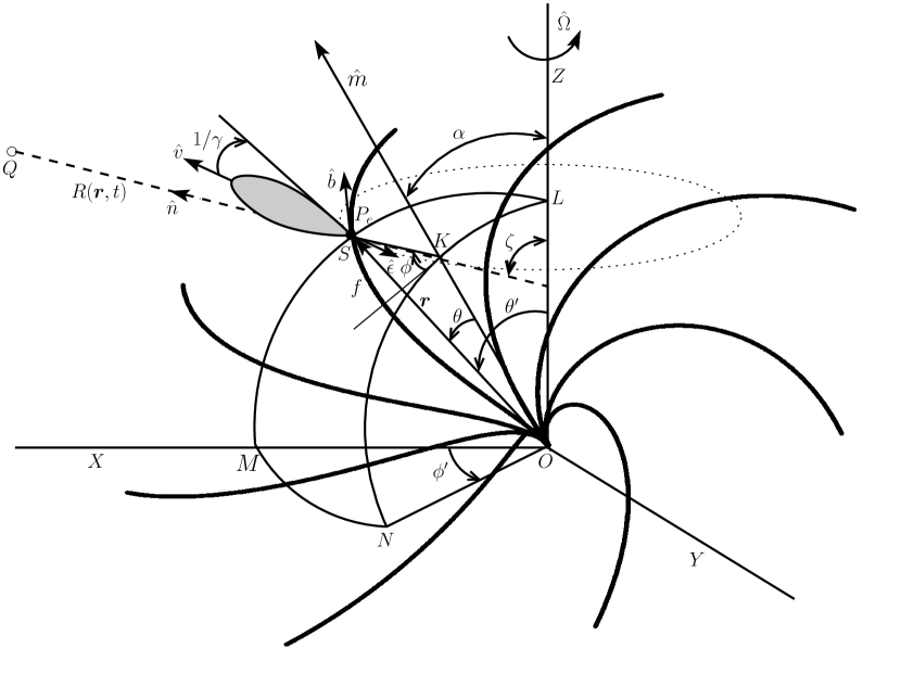
Figure 1: Geometry of curvature radiation in a rotating PC–current-perturbed magnetic dipole with the Cartesian coordinate system$-XYZ$ as an inertial observer’s frame whose origin is the neutron star center at $O.$ The magnetic axis $\hat{m}$ is inclined to the rotation axis $\hat{\Omega}$ by an angle $\alpha,$ and the rotation phase $\phi^{\prime}$ of the magnetic axis is measured from the fiducial $XZ-$ plane. The thick solid line curves represent the PC–current-perturbed field lines, and the parameters $\alpha=30^{\circ},$ $\phi^{\prime}=30^{\circ},$ field line constant $r_{e}=1r_{LC},$ pulsar rotation period $P=1$ s, a current scale factor $\varsigma=1,$ magnetic azimuth $\phi_{i}$ from $0^{\circ}$ to $360^{\circ}$ in steps of $45^{\circ}$, magnetic colatitude $\theta_{i}=0^{\circ}$, and emission altitude $r$ from $0$ to $0.8~{}r_{\rm LC}$ are used to sketch them. The unit vectors $\hat{b}$ and $\hat{\epsilon}$ represent the direction of perturbed field line tangent and pulsar rotation, respectively. The source net velocity $\hat{v}$ represent the direction of beamed radiation.

Let us consider a stationary Cartesian coordinate system–XYZ with the origin O located at neutron star center as an inertial observer frame (see Figure 1). Consider an inclined and rotating PC–current perturbed magnetic dipole with an inclination angle $\alpha$ with respect to the rotation axis $\hat{\Omega},$ which is taken to be parallel to Z-axis. The velocity $v$ of the relativistic source $S,$ which is constrained to move along the rotating PC–current perturbed dipole field line f, is given by

$$\mbox{\boldmath$v$}=\kappa c\,\hat{b}+\mathbf{\Omega}\times\textbf{r}~{},$$ (1)

where $\hat{b}=\mbox{\boldmath$B$}/|\mbox{\boldmath$B$}|$ and $\mbox{\boldmath$B$}=\mbox{\boldmath$B_{0}$}+\mbox{\boldmath$B_{1}$}.$ And $B_{0}$ is the unperturbed dipole field, $B_{1}$ is the PC–current-induced field, and r is the position vector of the source (KG, 2012b). The parameters $\mathbf{\Omega}=\Omega\hat{\Omega}$ is the pulsar angular velocity and $\kappa$ specifies the normalized speed of the source with respect to the speed of light c along the associated perturbed field line.

The first term on the r.h.s. of Equation (1) is the velocity of source along the perturbed field lines. The second term is the induced velocity due to corotation of the pulsar magnetosphere. Note that due to the PC–current-perturbation, the field lines which lie above the magnetic axis, tend to azimuthally twist towards the pulsar rotation, whereas those which lie below the magnetic axis, twist in the opposite directions (see Figure 1 in KG, 2012b). Therefore, the contributions to aberration of the source velocity $v$ by the above two terms add up for the negative sight line impact angle $\sigma,$ but they try to cancel each other for the positive $\sigma.$ However, since the aberration of source velocity due to the effect of rotation is larger than that due the PC–current-perturbation for the current which is of order Goldreich-Julian current, the net aberration will be always in the direction of pulsar rotation, and it is greater for negative $\sigma.$

Since the relativistic emissions are beamed in the direction of velocity $v$ with half-opening angle $1/\gamma,$ observer can receive the emissions only from a selected emission region whose boundary satisfies $\hat{n}\cdot\hat{v}=\cos(1/\gamma),$ where $\hat{v}=\mbox{\boldmath$v$}/|\mbox{\boldmath$v$}|$ and the sight line $\hat{n}=\left\{\sin\zeta,~{}0,~{}\cos\zeta\right\}$ with $\zeta=\alpha+\sigma.$ But the exact analytical solutions for the emission point coordinates $(\theta_{0},~{}\phi_{0})$ and $(\theta_{e},~{}\phi_{e})$ (see KG (2012a) and KG (2012b) for their definition) of the beaming region are hard to find once the effects of rotation and PC–current perturbation are considered, and hence we seek numerical solutions. Note that in finding exact values for coordinates $\theta_{0}$ and $\phi_{0},$ the values obtained from KG (2012b) have to be used as initial guess values for fast convergence unlike KG (2012a) wherein they have used those derived from Gangadhara (2010).

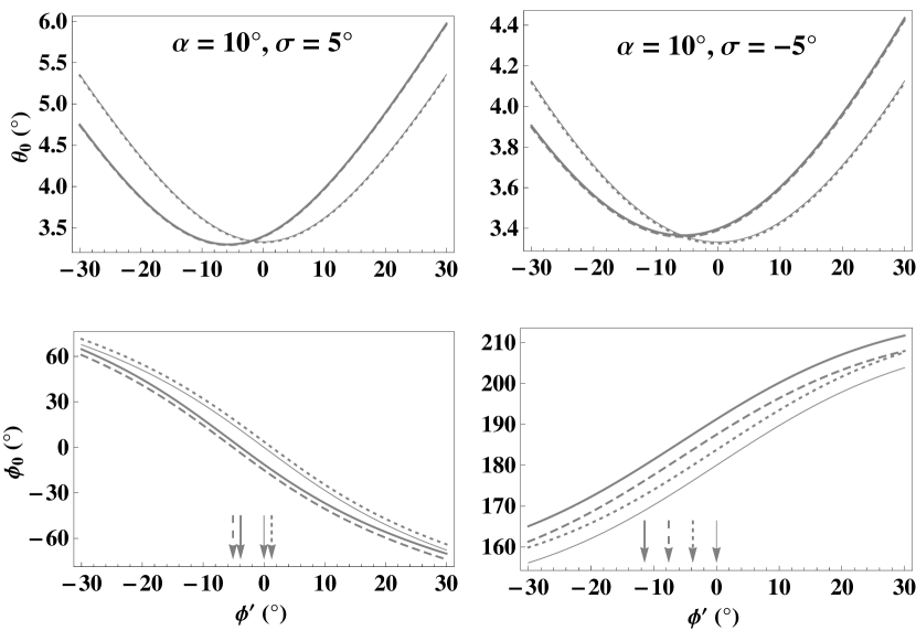
Figure 2: Emission point coordinates $\theta_{0}$ and $\phi_{0}$ as functions of rotation phase $\phi^{\prime}$ in the cases of nonrotating dipole (thin solid line curves), nonrotating PC–current-perturbed dipole (dotted line curves), rotating dipole (dashed line curves), and rotating PC–current-perturbed dipole (thick solid line curves). The arrows in the $\phi_{0}$ panels (line styled similar to $\phi_{0}$) indicate the antisymmetric point of $\phi_{0}$ in the respective cases. Here we used $r_{n}=0.1,$ $P=1$ s, $\gamma=400,$ and $\varsigma=1.$

By using the parameters $r_{n}=0.1,$ $P=1$ s, source Lorentz factor $\gamma=400,$ the current scale factor $\varsigma=1$, $\alpha=10^{\circ},$ and $\sigma=\pm 5^{\circ},$ we computed $\theta_{0}$ and $\phi_{0},$ and presented in Figure 2 as function of $\phi^{\prime}.$ Due to the PC–current perturbation alone (represented by dotted line curves), the emission points in $\phi_{0}$ shift to later phases for positive $\sigma$ and to the earlier phases for negative $\sigma,$ whereas they are mostly unaffected in $\theta.$ On the other hand due to the effect of rotation (aberration) alone (represented by dashed line curves), the emission shifts to earlier phases in both $\theta$ and $\phi.$ However the phase shift of emission points in $\phi$ caused due to rotation alone is larger than that due to PC–current perturbation alone. This can be clearly seen in the phase shifts of the antisymmetric point of $\phi_{0}$ (phase at which $\phi_{0}$ is equal to $0^{\circ}$ or $180^{\circ}$) indicated by arrows (styled same as $\phi_{0}$). As a result, in the more realistic case of rotating PC–current perturbed dipole (represented by thick solid line curves), the emission points in $\theta$ shift to earlier phases in both the cases of $\sigma$ by the same amount as that in the case of rotating dipole, whereas in $\phi,$ they shift to the earlier phases by a smaller amount in the case of positive $\sigma$ and by larger amount in the case of negative $\sigma.$ Note that, if the emission region is modulated (nonuniform source distribution) in the azimuthal direction which we show later, then the resulted intensity components will also show aforesaid asymmetric phase shift between the positive and negative $\sigma$ cases.

We also computed $\theta_{0}$ and $\phi_{0}$ for the case of rotating perturbed dipole by assuming $\theta_{0}=\theta_{0}^{\prime}+\delta\theta_{\rm rot}+\delta\theta_{\rm pcc},$ and $\phi_{0}=\phi_{0}^{\prime}+\delta\phi_{\rm rot}+\delta\phi_{\rm pcc},$ where $\theta_{0}^{\prime}$ and $\phi_{0}^{\prime}$ are the coordinates of emission points in the nonrotating unperturbed dipole. The changes in the colatitude $\delta\theta_{\rm rot}=\theta_{0,\rm rot}-\theta_{0}^{\prime}$ and $\delta\theta_{\rm pcc}=\theta_{0,\rm pcc}-\theta_{0}^{\prime}$ and those in the azimuth $\delta\phi_{\rm rot}=\phi_{0,\rm rot}-\phi_{0}^{\prime}$ and $\delta\phi_{\rm pcc}=\phi_{0,\rm pcc}-\phi_{0}^{\prime}$ are due to the aberration and PC–current perturbation, respectively. The parameters $\theta_{0,\rm rot}$ and $\theta_{0,\rm pcc}$ are the coordinates after separately considering the perturbations: rotation and PC–current, respectively, and similarly $\phi_{0,\rm rot}$ and $\phi_{0,\rm pcc}.$ We find that thus obtained $\theta_{0}$ and $\phi_{0}$ more or less match with the thick solid line curves (not shown in the Figure). Therefore, the phase shifts as well as the changes in the magnitude of emission point coordinates $\theta_{0}$ and $\phi_{0}$ due to the two separate perturbations (rotation and PC–current), simply add up when the two effects are combined together.

The acceleration of source is given by

$$\mbox{\boldmath$a$}=\frac{(\kappa c)^{2}}{|\mbox{\boldmath$b$}|}\frac{d\hat{b}}{d\theta}+\frac{\kappa c^{2}}{|\mbox{\boldmath$b$}|}\frac{d\kappa}{d\theta}\hat{b}+2\kappa c(\mbox{\boldmath$\Omega$}\times\hat{b})+\mbox{\boldmath$\Omega$}\times(\mbox{\boldmath$\Omega$}\times\textbf{r})~{},$$ (2)

where we have used the expression of arc length of the field line $ds=|\mbox{\boldmath$b$}|d\theta=\kappa c~{}dt,$ and the total derivative $dF/d\theta=\partial F/\partial\theta+(\partial F/\partial\phi)(d\phi/d\theta),$ where $F$ stands for $\hat{b},$ $\kappa,$ etc. The first term on r.h.s. of Equation (2) is the acceleration of bunch due to curvature of the PC–current perturbed field lines. Note that it includes both the intrinsic curvature due to the dipolar field and the induced curvature due the PC-current perturbation on the dipole field. The small change in the source speed due to motion along the perturbed field line is represented by the second term and it is tiny among other terms. The third term is the rotationally induced acceleration due to the Coriolis force and is in the direction of pulsar rotation. The last term is the induced acceleration due to the Centrifugal force which is acting away from the rotation axis. The PC–current-induced acceleration which is included in the first term becomes much important at higher emission altitude, larger pulsar angular velocity, and smaller $\alpha.$ On the other hand, the Coriolis and the centrifugal accelerations with the Coriolis term being the dominant one become much important at higher emission altitude, larger pulsar angular velocity, but at larger $\alpha.$

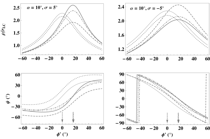
Figure 3: Radius of curvature $\rho$ of source trajectory, and position angle $\psi$ of the radiation electric field as functions of $\phi^{\prime}.$ The lines representation is the same as in Figure 2. The dot-dashed line curves represent the parameters obtained by simple addition of the two perturbations due to the rotation and the PC–current. The thin dot-dashed line curve in the $\psi$ panels represents the analytical perturbation theory (Hibschman & Arons, 2001) whereas the thick dot-dashed line curve represents our numerical result. The arrows in the $\psi$ panels (styled same as $\psi$) represent the inflection point of $\psi.$ For simulation we used the parameters which are the same as in Figure 2.

By using the parameters, which are the same as in Figure 1, we computed the radius of curvature $\rho\approx v^{3}/|\mbox{\boldmath$v$}\times\mbox{\boldmath$a$}|$ as a function of $\phi^{\prime}$, and plotted in upper panels of Figure 3. The PC–current perturbation (represented by the dotted line curves) leads to larger curvature with respect the unperturbed ones (thin solid line curve) leaving the symmetric point of $\rho$ to be mostly unaffected (KG, 2012b). On the other hand, rotation induces an asymmetry into the curvature between the leading and trailing sides of $\phi^{\prime}=0^{\circ},$ since the leading side trajectory becomes more curved and $\rho$ maximum shifts to the trailing side (e.g., KG, 2012a). Since the perturbation due to PC–current in the case of positive $\sigma$ opposes that due to the corotation, the net $\rho$ in the rotating PC–current perturbed dipole (thick solid line curve) becomes larger than that due to rotation alone, and vice versa in the case of negative $\sigma.$

To assess the possibility of deriving $\rho$ for the rotating PC–current perturbed dipole by considering separately the perturbations due to PC–current and rotation, analogues to the $\theta_{0}$ and $\phi_{0}$ in Figure 2, we considered the net curvature as $\mbox{\boldmath$k$}=\mbox{\boldmath$k^{\prime}$}+\mbox{\boldmath$\delta k_{\rm rot}$}+\mbox{\boldmath$\delta k_{\rm pcc}$},$ where $k^{\prime}$ is the curvature of the unperturbed dipolar field lines, $\mbox{\boldmath$\delta k_{\rm rot}$}=\mbox{\boldmath$k_{\rm rot}$}-\mbox{\boldmath$k^{\prime}$}$ and $\mbox{\boldmath$\delta k_{\rm pcc}$}=\mbox{\boldmath$k_{\rm pcc}$}-\mbox{\boldmath$k^{\prime}$}.$ The $k_{\rm rot}$ and $k_{\rm pcc}$ are the curvature vectors in the cases of rotating dipole and PC–current perturbed dipole, respectively. The resultant $\rho$ can be derived as

$$\rho=\left[\frac{1}{\rho^{\prime 2}}+\frac{1}{\rho_{\rm rot}^{2}}+\frac{1}{\rho_{\rm pcc}^{2}}-2\left(\frac{\hat{a}^{\prime}\cdot\hat{a}_{\rm rot}}{\rho^{\prime}~{}\rho_{\rm rot}}+\frac{\hat{a}^{\prime}\cdot\hat{a}_{\rm pcc}}{\rho^{\prime}~{}\rho_{\rm pcc}}-\frac{\hat{a}_{\rm rot}\cdot\hat{a}_{\rm pcc}}{\rho_{\rm rot}~{}\rho_{\rm pcc}}\right)\right]^{-1/2},$$ (3)

where $\rho^{\prime},$ $\rho_{\rm rot},$ and $\rho_{\rm pcc}$ are the radii of curvature and $\hat{a}^{\prime},$ $\hat{a}_{\rm rot},$ and $\hat{a}_{\rm pcc}$ are the unit acceleration vectors in the cases of non-rotating dipole, rotating dipole and PC–current perturbed dipole, respectively. Thus obtained $\rho,$ by adding the two separate perturbations computed independently, is superposed in $\rho$ panels of Figure 3 (see the dot-dashed line curves). We can see that, it is significantly different from the actual $\rho$ of the rotating PC–current perturbed dipole.

The polarization position angle $\psi$ of the electric field of radiation due to relativistic sources, defined as the angle between the radiation electric field and the projected spin axis on the plane of the sky, can be computed by knowing the acceleration of the radiation source: $\tan\psi=\hat{\epsilon}_{\perp}\cdot\hat{a}/(\hat{\epsilon}_{\parallel}\cdot\hat{a}),$ where $\hat{\epsilon}_{\parallel}$ (projected spin vector) and $\hat{\epsilon}_{\perp}$ are unit vectors in the directions perpendicular to $\hat{n}$ (Gangadhara, 2010). By using the parameters which are same as in upper panels of Figure 3, we computed the position angle $\psi$ as a function of $\phi^{\prime},$ and plotted in lower panels of Figure 3. The perturbation due to the PC–current (represented by dotted line curves) causes the $\psi$ curve to shift upward with respect to the standard RVM curve (nonrotating dipole, thin solid line curve) while its inflection point remain unaffected (Hibschman & Arons, 2001; KG, 2012b). On the other hand the rotation (aberration) causes the $\psi$ curve to shift upward or downward, depending upon sign of $\sigma$, and always shifts the inflection point to the trailing side. Therefore in a more realistic case of rotating PC–current perturbed dipole the net $\psi$ will be shifted upward with respect to the one in rotating case, while the inflection point lies mostly at the same phase as in the rotating dipole.

We have also computed $\psi$ for the rotating perturbed dipole by assuming $\psi=\psi^{\prime}+\delta\psi_{\rm rot}+\delta\psi_{\rm pcc},$ where $\psi^{\prime}$ is due to the nonrotating dipole, $\delta\psi_{\rm rot}=\psi_{\rm rot}-\psi^{\prime}$, and $\delta\psi_{\rm pcc}=\psi_{\rm pcc}-\psi^{\prime}$ with $\psi_{\rm rot}$ and $\psi_{\rm pcc}$ are being the position angles after considering the perturbation separately due to rotation and PC–current, respectively. We find that thus obtained $\psi$ in both numerical (represented by thick dot-dashed line curves) and analytical perturbation theory (represented by thin dot-dashed line curves, see the Equations (D13) and (G11) in Hibschman & Arons, 2001) significantly differ from the actual $\psi$ of the rotating PC–current-dipole. Therefore we believe that the two effects have to be combined together in deducing the polarization state of the radiation field.

3 POLARIZATION STATE OF THE RADIATION FIELD

The radiation emitted by the relativistic accelerating sources will have a broad spectrum, and it is given by (Jackson, 1998):

$$\textbf{E}(\textbf{r},\omega)=\frac{1}{\sqrt{2\pi}}\frac{qe^{i\omega R_{0}/c}}{R_{0}~{}c}\int^{+\infty}_{-\infty}\frac{|\textbf{b}|}{\kappa c}\frac{\hat{n}\times[(\hat{n}-\mbox{\boldmath$\beta$})\times\mbox{\boldmath$\dot{\beta}$}]}{\xi^{2}}e^{i\omega(t-\hat{n}\cdot\textbf{r}/c)}d\theta.$$ (4)

Note that the time $t$ in the above equation has to be replaced by the expression given in Equation (6) of KG (2012a), and the parameters $\phi^{\prime}$ by $\Omega~{}t$ and $\phi$ by the expression given in Equation (11) of KG (2012b). We solve the integral using the method given in KG (2012a) and find the polarization state of the radiation field in terms of the Stokes parameters $I,$ $Q,$ $U$ and $V.$

3.1 Emission from Uniform Distribution of Sources

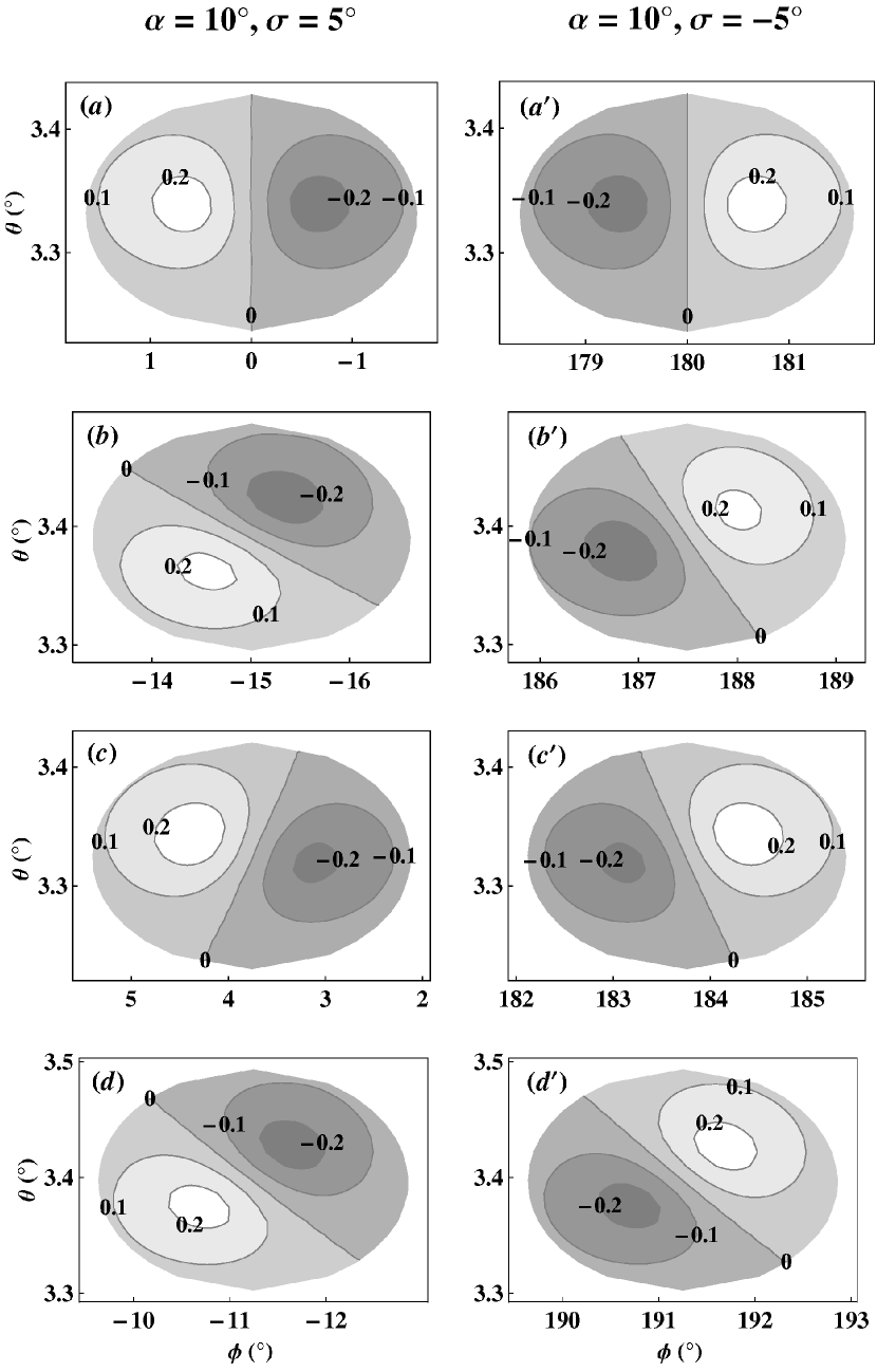
Figure 4: The pattern of the circular polarization for the emissions from the beaming region with the uniform distribution of sources in the cases: the nonrotating dipole$-$panels $(a)$ and $(a^{\prime});$ rotating dipole$-$panels $(b)$ and $(b^{\prime});$ nonrotating PC–current-perturbed dipole$-$panels $(c)$ and $(c^{\prime});$ and rotating perturbed dipole$-$panels $(d)$ and $(d^{\prime}).$ In each panel, emissions are normalized with the corresponding maximum of the total intensity. Here, we used the parameters $\phi^{\prime}=0^{\circ},$ $\nu=600$ MHz and the rest are the same as in Figure 2.

By assuming an uniform distribution of sources throughout the emission region, we computed the radiation field from the beaming region and its polarization state, and presented in Figure 4. Since the magnitude of rotation of contour patterns of the total intensity and the linear polarization in $(\theta,\phi)-$ are more or less the same as that of the circular polarization, we present only the contour patterns of circular polarization. However, the total intensity and linear polarization will be maximum at the beaming region center and fall considerably towards the boundary with a slightly larger emission towards the larger curvature region (see Figure 3 in KG, 2012a, b).

Due to pulsar rotation, the contour patterns of the circular polarization (panels $b,~{}b^{\prime})$ gets rotated in $(\theta,~{}\phi)$–plane with respect to those in the nonrotating dipole (panels $a,~{}a^{\prime}),$ and the rotation is from the trailing side to the leading side for both the signs of $\sigma.$ Further there arises an asymmetry in the strength of the positive and negative polarities of the circular polarization in such a way that the negative circular gets quite stronger. On the other hand due to the PC–current perturbation, the rotation direction of the contour patterns of the circular polarization (panels $c,~{}c^{\prime}$) becomes opposite between the positive and negative $\sigma$ cases. That is for the positive $\sigma$ it is opposite to that due to the effect of rotation, whereas it is in the same direction for the negative $\sigma.$ However the magnitude of rotation of the contour patterns due to the PC–current is smaller than that due to the pulsar rotation. Also, due to the PC–current, the positive polarity of the circular polarization becomes stronger than the negative polarity for both $\pm\sigma.$ Therefore, in the case of rotating PC–current perturbation (panels $d,~{}d^{\prime}$), the rotation direction of the contour pattern of the circular polarization will be in the same direction as that in the panels $(b)$ and $(b^{\prime})$ but with the lower magnitude of rotation for the positive $\sigma$ than for negative $\sigma.$ Further, due to the opposite selective enhancement of either the positive or negative polarity of the circular polarization by the two perturbations (rotation and PC–current), the circular polarization becomes more or less have same strength between the positive and negative polarities, in similarity with the nonrotating case.

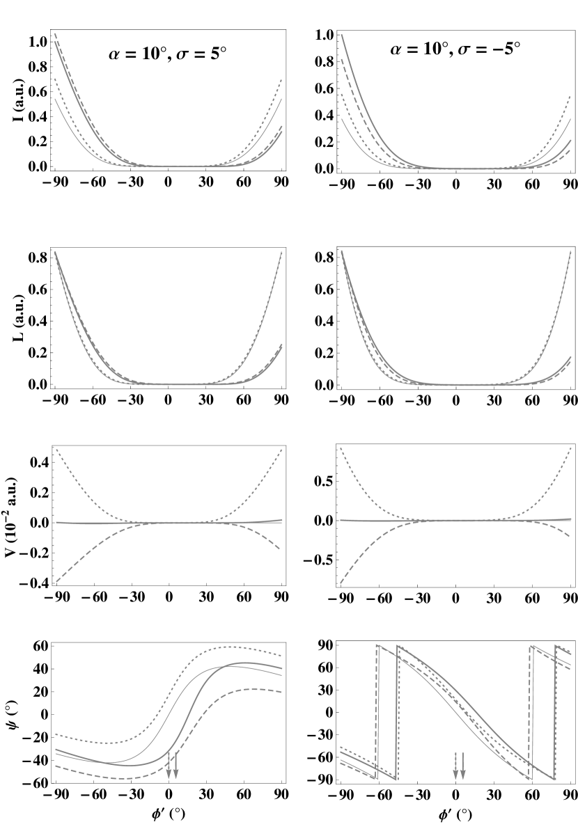
Figure 5: Simulations showing the emission with uniform distribution of sources before and after considering the perturbations due to the rotation and PC–current (the lines style is the same as in Figure 2). In $I$ panels, the emissions are normalized with the corresponding maximum of the total intensity after combining the the two perturbations, whereas in $L$ and $V$ panels, they are normalized with the corresponding maximum of $I$ in the respective cases. The arrows in the $\psi$ panels (styled the same as $\psi)$ indicate the PPA inflection points. Used $\nu=600$ MHz and the rest are the same as in Figure 2.

Emissions from the beaming region due to different plasma bunches will be incoherently added at the observation point if they are separated by a space larger than the radiation wavelength. Hence, the resultant emission that the observer receives will be the sum of the intensities from the different plasma bunches. Using the expressions given in Gangadhara (2010, from Equation 33 to Equation 36), we computed the polarization state of the emitted radiation due to uniform distribution of sources, and they are presented in Figure 5. With the uniform distribution of sources, the PC–current perturbation alone (represented by the dotted line curves) does not affect the symmetry of the total intensity $I$ between the leading and trailing sides of $\phi^{\prime}=0^{\circ}$ which is similar to the nonrotating dipole, whereas the rotation introduces an asymmetry (represented by the dashed line curves) with the leading side becomes stronger due to an induced larger curvature of source trajectory on the leading side (see Figure 3). In the more realistic rotating perturbed dipole, there remains an asymmetry similar to the case of rotating dipole, however with the emission that is significantly differs from that in the cases of the rotating dipole and the PC–current perturbed dipole when considered separately.

Due to an incoherent addition of emissions from the different bunches within the beaming region the magnitude of linear polarization $L$ become bit smaller than that of total intensity $I$. However, the profile of $L$ more or less matches with the corresponding $I.$ The net survived circular polarization $V$ in the case of rotating perturbed dipole (represented by the thick solid line curves) becomes very tiny because of the two perturbations (rotation and PC–current), which selectively enhance the opposite polarities of $V$ as shown in Figure 4. The position angle is increasing in the case of positive $\sigma$ whereas it is decreasing in the case of negative $\sigma$ with the inflection point always shifted to trailing side.

3.2 Emissions Due to Nonuniform distribution of Sources

We considered a Gaussian modulation function that is given in KG (2012a, b) to model the nonuniform distribution of sources in the emission region. We find the polarization state of the radiation field from the nonuniform distribution of sources using the expressions given in Gangadhara (2010) (see equations 38 of Gangadhara, 2010).

3.2.1 Emission with Azimuthal Modulation

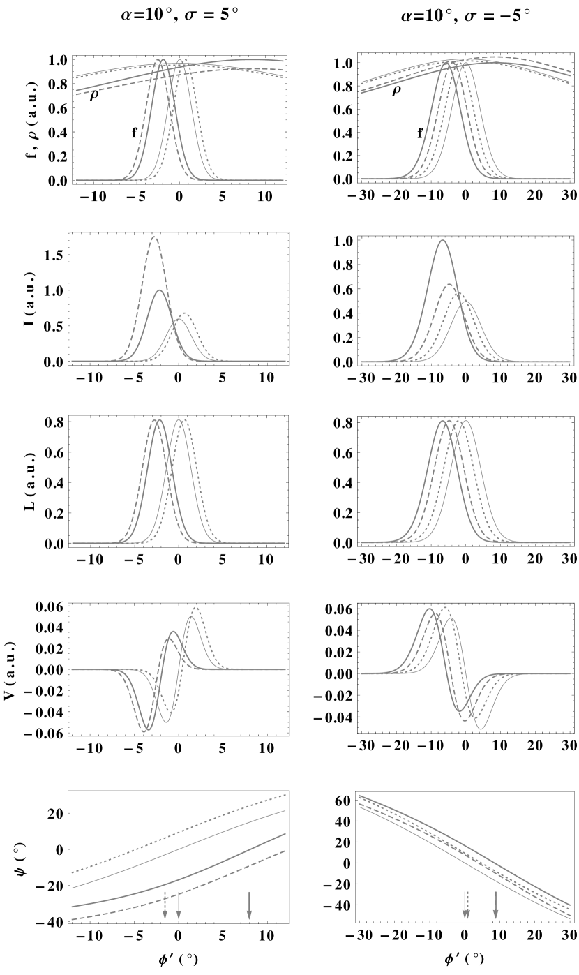
Figure 6: Simulated pulse profiles with modulation in the azimuthal direction. The total intensity $I$ is normalized with the maximum of $I$ of the combined case of rotation and PC–current, whereas $L$ and $V$ are normalized with the corresponding maximum of $I$ in the respective cases. We used $r_{n}=0.05,$ $f_{\theta}=1,$ $\phi_{P}=0^{\circ},$ and $\sigma_{\phi}=0.1$. The rest parameters are the same as in Figure 5.

By considering a modulation in the magnetic azimuth with the peak at the meridional plane, we simulated the polarization profiles affected by the rotation and PC–current perturbations, and plotted in Figure 6 along with the profiles of unperturbed emissions. We chose $r_{n}=0.05,$ $f_{\theta}=1,$ $\phi_{P}=0^{\circ},$ $\sigma_{\phi}=0.1$ and the rest parameters the same as in Figure 5. We can see that due to perturbations both the emission and polarization significantly get affected in phase and magnitude, however, the maximum of $L$ mostly remain unaffected. Pulsar rotation causes the intensity components to get shifted to the earlier phases with respect to the fiducial plane, whereas the PPA inflection points to later phases for both the signs of $\sigma.$ On the other hand PC–current causes the intensity components shift to later phases and the PPA inflection point to earlier phases for the positive $\sigma$ and vise versa for the negative $\sigma.$

The net phase shift of intensity component and that of the PPA inflection point after combining the two perturbations are found to be $-2^{\circ}.16$ and $7^{\circ}.95,$ respectively in the case of $\sigma=5^{\circ},$ whereas they are found to be $-6^{\circ}.69$ and $8^{\circ}.90,$ respectively in the case of $\sigma=-5^{\circ}.$ On the other hand, the sum of the phase shifts of the intensity components caused separately by the rotation and PC–current are found to be $-2^{\circ}.10$ and $-6^{\circ}.87$ respectively in the cases of $\sigma=\pm 5^{\circ},$ whereas that of the PPA inflection point are found to be $6^{\circ}.44$ and $9^{\circ}.59,$ respectively. Therefore, the absolute relative difference between the phase shift of intensity component that resulted when the two perturbations taken together and that due to the sum of two separate perturbations, is about $<3\%$ in both the cases of $\sigma,$ whereas that for the PPA inflection point is found to be about $19\%$ in the case of $\sigma=5^{\circ},$ and $8\%$ in the case of $\sigma=-5^{\circ}.$ Note that the net phase shift of the intensity component becomes slightly larger than that of the net modulation $f$ (which is about $-1^{\circ}.92$ and $-5^{\circ}.71,$ respectively in the cases of $\sigma=\pm 5^{\circ}$) due to an induced asymmetry in the net radius of curvature about the peak location of modulation.

Although circular polarization of opposite polarities from the background unmodulated emission roughly cancels out, a net circular however with an asymmetry between the opposite polarities survives in the presence of modulation. This is because of an asymmetry in the magnitude of rotation of the emission pattern with respect to rotation phase in such a way that larger rotation magnitude towards the inner rotation phases as compared to that on outer phases (KG, 2012a). Hence, it results in the selective enhancement of the leading side circular over the trailing side circular. However, the asymmetry between the opposite polarities of the circular polarization becomes smaller for the positive $\sigma$ than that for the negative $\sigma.$ This is due to an opposite behavior of PC–current in introducing an asymmetry between the opposite polarities of $V$ between the $\pm\sigma$ wherein it selectively enhances the trailing positive circular for $+\sigma$ whereas the leading positive circular for $-\sigma.$ On the other hand pulsar rotation causes the selective enhancement of the leading polarity of $V,$ i.e., negative circular for $+\sigma$ and positive circular for $-\sigma.$

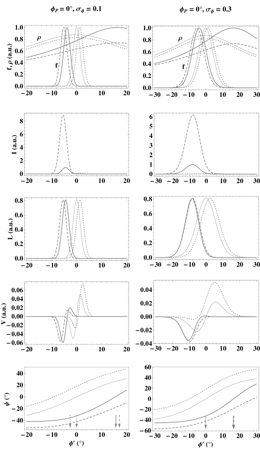
Figure 7: Same as Figure 6 except $r_{n}=0.1,$ $\sigma=5^{\circ}$ and two types of modulation: narrower $(\sigma_{\phi}=0.1)$ and broader $(\sigma_{\phi}=0.3)$ Gaussians are considered.

To assess whether we can estimate the net phase shift of intensity components by adding the phase shift due to each perturbation computed separately, we chose emission altitude $r_{n}=0.1,$ and two cases of modulation: narrower $(\sigma_{\phi}=0.1)$ and broader $(\sigma_{\phi}=0.3).$ The simulated pulses are presented in Figure 7. The net phase shift of the component after combining the two perturbations in the cases of $\sigma_{\phi}=0.1$ and $0.3$ are found to be $-4^{\circ}.40$ and $-8^{\circ}.33,$ respectively, whereas the PPA inflection point phase shifts are found to be $15^{\circ}.70$ and $16^{\circ}.23,$ respectively. On the other hand the sum of the phase shifts of the intensity components caused due to the two perturbations considered separately are found to be $-4^{\circ}.09$ and $-5^{\circ}.77$ respectively wherein the relative difference are about $7\%$ and $30\%$ respectively. For PPA inflection point the corresponding phase shifts are found to be $14^{\circ}.52$ and $16^{\circ}.52,$ respectively, wherein the absolute relative differences are about $7.5\%$ and $2\%,$ respectively. Hence the actual phase shifts of intensity components and PPA inflection point will be significantly different from those obtained when the two perturbations dealt separately.

In the case of $\sigma_{\phi}=0.1,$ the asymmetry in the strength of circular polarization between the opposite polarities become larger as compared to that in the lower altitude emission (see Figure 6). This is due to an increased asymmetry in the magnitude of rotation of beaming region emission pattern between the inner and outer phases wherein the small amount of rotation occurs at the outer phases. In the case of $\sigma_{\phi}=0.3,$ only the leading negative polarity of the circular polarization survives due to aforementioned reasons but this time it is enhanced more due to broader modulation and hence broader pulse width. Hence it results in the “symmetric”-type circular polarization.

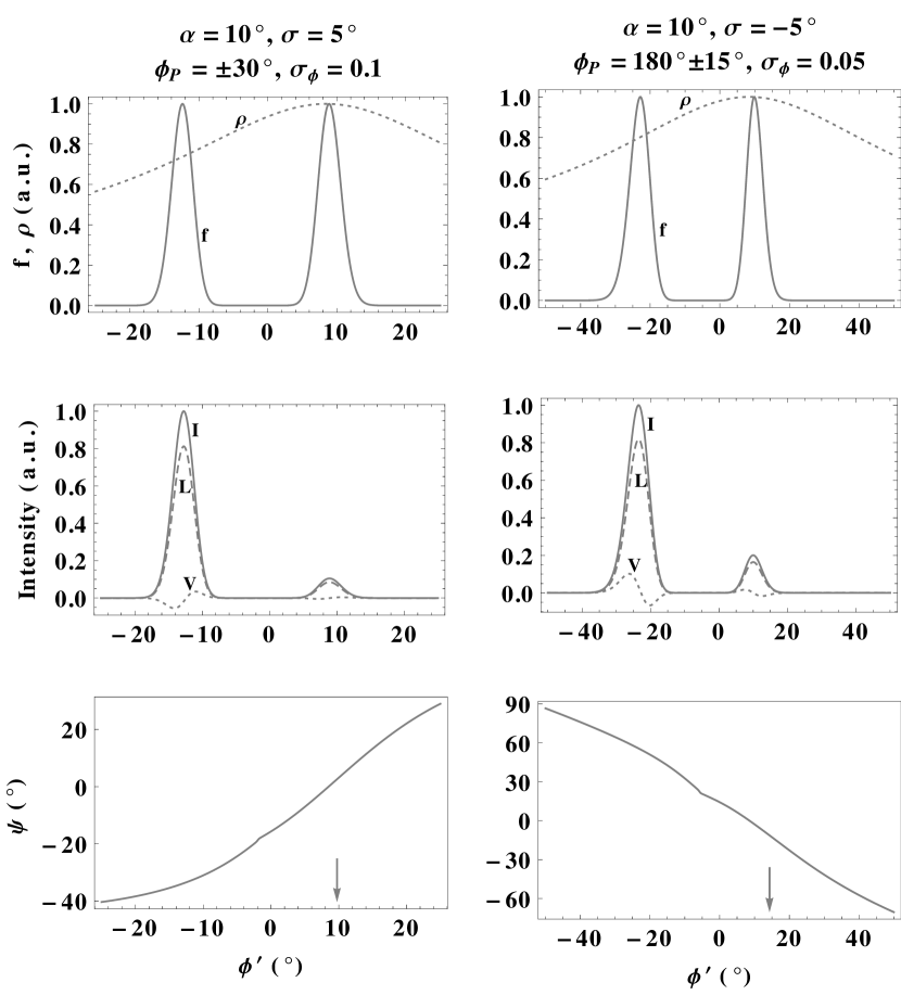
Figure 8: Same as Figure 6 but with two symmetrically located Gaussian modulations with respect to magnetic meridian plane and only the combined case of rotation and PC–current perturbations is presented. In the upper panels: $\rho-$dotted line curves, $f-$solid line curves; in the intensity panels: $I-$ solid line curves, $L-$dashed line curves, $V-$ dotted line curves.

As a case of modulation which lies symmetrically on either side of the meridional plane, we choose the modulation peaks located at $\phi_{P}=\pm 30^{\circ}$ for $\sigma=5^{\circ}$ and $\phi_{P}=180^{\circ}\pm 15^{\circ}$ for $\sigma=-5^{\circ},$ and the simulated profiles are given in Figure 8. Note that only the combined case of rotation and PC–current perturbations is given in all panels. Although an observer encounters mostly the same plasma density (modulation strength) between the leading and trailing sides, the net modulated intensity component on the trailing side becomes weaker than that on the leading side due to the induced larger curvature of source trajectory on the leading side. Further the leading side component becomes broader than the trailing one due to an induced asymmetry in the sight line encountered modulation and that in the gradient of radius of curvature. The behaviors of linear and circular polarization are same as in the Figure 6 except the enhancement of trailing part of the circular polarization in the trailing side components.

3.2.2 Emission with Polar Modulation

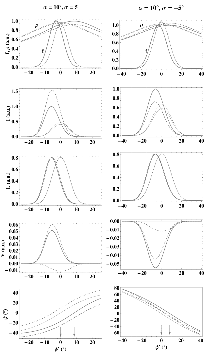
Figure 9: Same as Figure 6 but with the nonuniform distribution of sources in the polar direction and $f_{\phi}=1$, $\theta_{P}=2^{\circ},$ and $\sigma_{\theta}=0.01$.

By considering a modulation with plasma density gradient in the polar direction we present the effects of rotation and PC–current perturbation on pulsar emission and polarization. In Figure 9, we present the simulation of hallow cone emissions surrounding the magnetic axis with modulation peak at $\theta_{P}=2^{\circ}.$ Since the minimum of $\theta_{0}$ is about $\sim(2/3)\sigma$ which is about $3^{\circ}.3$ for $\sigma=\pm 5^{\circ},$ observer’s sight line cuts the hollow cone emission only once in each pulsar rotation, and hence it results in a single component profile. For the sake of comparison, the cases of before and after consideration of the perturbations are all shown in the Figure 9, and the parameters normalization and the line representations are the same as in Figure 6. Note that, unlike the case of azimuthally modulated emissions (see Figure 6), the maximum of modulation strength that the observer encounters in the lab frame is not same in all the cases as the minimum of $\theta_{0}$ slightly get affected due to the perturbations. But, similar to the case of Figure 6, the emissions get affected significantly before and after considering the perturbations due to the induced differences in $\rho$ at the peak locations of $f.$ The net phase shifts of a component after combining the two perturbations in the cases of $\sigma=\pm 5^{\circ}$ are found to be $-5^{\circ}.79$ and $-6^{\circ}.29,$ respectively. On the other hand the net phase shift obtained by adding the phase shifts due to the rotation and PC–current when considered separately in the cases of $\sigma=\pm 5^{\circ}$ are found to be $-5^{\circ}.32$ and $-6^{\circ}.83,$ respectively. Hence the relative differences are about $8\%$ and $8.5\%,$ respectively with respect to the combined case of the perturbations. Note that this relative differences in the intensity phase shifts become larger at higher altitude $(\sim r_{n}=0.1).$

The maximum of normalized linear polarization $L$ is more or less the same in all the cases, similar to Figure 6. Although the position angle significantly gets affected after combining the two perturbations, its inflection point lies at roughly the same phase as that due to the rotation alone. The circular polarization $V$ becomes symmetric type with the opposite polarities survive due to an opposite direction of rotation of emission pattern in the beaming region. The net circular polarization after combining the two perturbations will also be symmetric type with the survival of polarity as that due to the pulsar rotation alone.

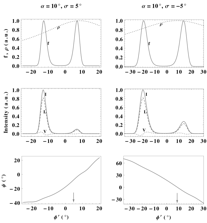
Figure 10: Same as Figure 9 with the combined effect of rotation and PC–current (the line style is the same as in Figure 8) except with the parameters $\theta_{P}=3^{\circ}.6$ and $\sigma_{\theta}=0.002.$

By considering a hallow cone modulation with peak at $\theta_{P}=3^{\circ}.6,$ we have analyzed a case where the sight line cuts the hallow cone emission twice (see Figure 10). Similar to Figure 8, the trailing side intensity component become weaker as well as narrower than that on the leading side, due to the induced asymmetry in the curvature of source trajectories between the two sides. Since the sight line crosses the central maximum of the hallow cone on both the leading and trailing sides, there is a change over of selective enhancement of emission over the part of the beaming region with smaller values of $\theta$ to that over the larger values $\theta$ on the leading side, and vice versa on the trailing side. Hence, there results an antisymmetric circular polarization with the sign reversal from positive to negative over in leading side component and vice versa on the trailing side for the case of positive $\sigma.$ On the other hand, it is vice versa for the case of negative $\sigma$ due to the opposite direction of rotation of the emission pattern of the beaming region.

3.2.3 Emission with Modulation in both Azimuthal and Polar directions

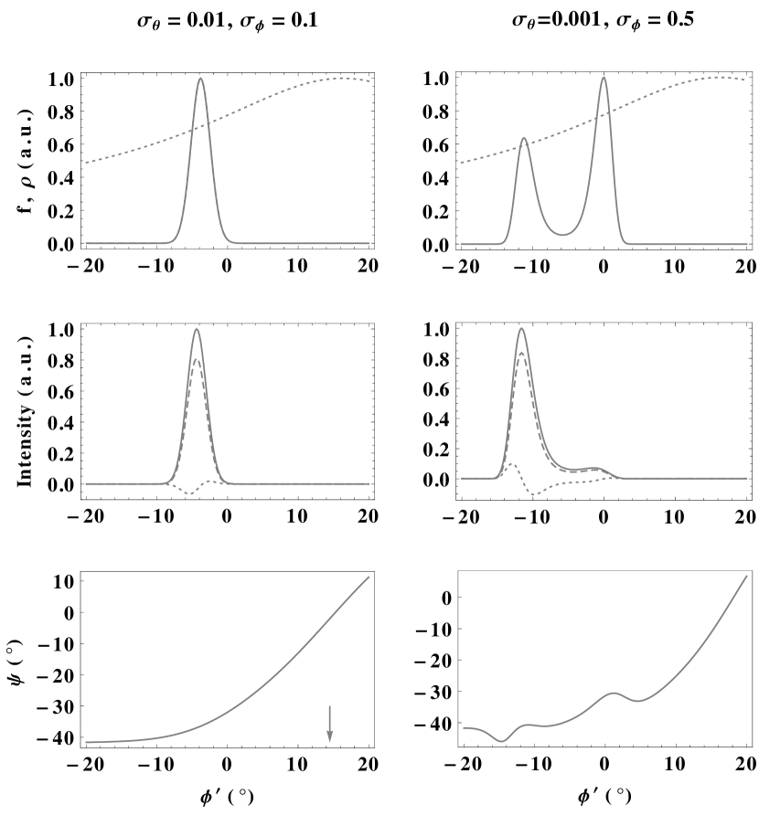
Figure 11: Simulated pulse profiles with the nonuniform distribution of sources in both the polar and azimuthal directions, after considering the perturbations by the rotation and PC–current. The line style is the same as in Figure 8. We chose $\sigma=5^{\circ},$ $r_{n}=0.1,$ $f_{0}=1,$ $\theta_{p}=3^{\circ}.4,$ $\phi_{P}=0^{\circ},$ and the rest parameters are the same as in Figure 5.

The radiation sources may be nonuniformly distributed in both the polar and azimuthal directions in the pulsar magnetosphere. The extreme cases, wherein the modulation is predominant in azimuthal or polar directions are already discussed in Sections $3.2.1.$ and $3.2.2.,$ respectively. In this section we present a few more cases where the modulation exists in both the polar and azimuthal directions. In Figure 11, we considered the cases $\sigma_{\theta}=0.01$ and $\sigma_{\phi}=0.1$ wherein the modulation is effectively dominating in the azimuthal direction over that in the polar direction, and $\sigma_{\theta}=0.001$ and $\sigma_{\phi}=0.5$ wherein the modulation becomes effective in $\theta.$ Note that in the case of $\sigma_{\theta}=0.01$ and $\sigma_{\phi}=0.1,$ even though $\sigma_{\theta}<\sigma_{\phi},$ the modulation becomes effective in $\phi$ coordinate than in $\theta$ due to the much larger coverage of $\phi$ compared to that of $\theta,$ see for e.g., Figures 3 and 4. In the case of $\sigma_{\theta}=0.01$ and $\sigma_{\phi}=0.1,$ the emission and polarization properties are similar to the case of $\alpha=10^{\circ}$ and $\sigma=5^{\circ}$ of Figure 6 with an antisymmetric circular polarization wherein the sign reversal is from the negative polarity to the positive. On the other hand even though the single modulation is considered in the case of $\sigma_{\theta}=0.001$ and $\sigma_{\phi}=0.5$ but due to the viewing geometry, much elongation of the modulation in the azimuthal direction and squeezing into a narrow cone, the modulation encountered by the sight line results in a blended two components like structure. It further results into a two components like structure in intensity profile, however, with much weaker trailing side due to the larger $\rho.$ Although circular polarization is still antisymmetric type, the sign reversal becomes opposite to the case of $\sigma_{\theta}=0.01$ and $\sigma_{\phi}=0.1,$ i.e., from positive to negative, which is similar to the case of $\alpha=10^{\circ}$ and $\sigma=5^{\circ}$ in Figure 9. Hence in the presence of perturbations, it is hard to see the correlation between the sign reversal of circular polarization and the PPA swing as both the types of circular sign reversal seems to be associated with the increasing PPA swing. Note that, the inflection point of PPA swing is not derived in the case of $\sigma_{\theta}=0.001$ and $\sigma_{\phi}=0.5$ due to the difficulty in finding it because of the kinky nature in the PPA swing.

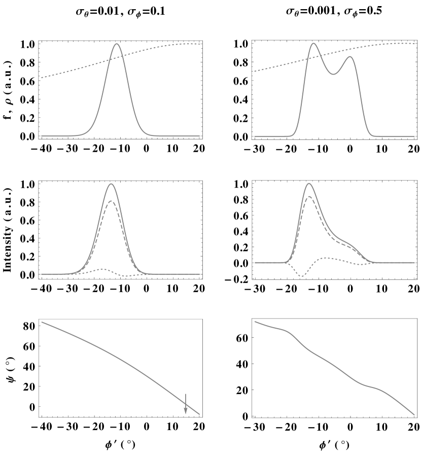
Figure 12: Same as Figure 11 except with $\sigma=-5^{\circ}$ and $\phi_{P}=180^{\circ}.$

By using $\sigma=-5^{\circ},$ $\phi_{P}=180^{\circ}$ and the rest parameters the same as in Figure 11, we computed the polarization profiles and plotted in Figure 12. In both cases of modulation, the profiles are similar to those in Figure 11 except with the opposite sign reversal of the circular polarization in the respective cases and decreasing PPA swing. Also, similar to Figure 11, due to perturbations no correlation is found between the sign reversal of the circular polarization and the PPA swing, as both the sign reversal of the circular polarization, i.e., from positive to negative or vice versa, are associated with the decreasing PPA.

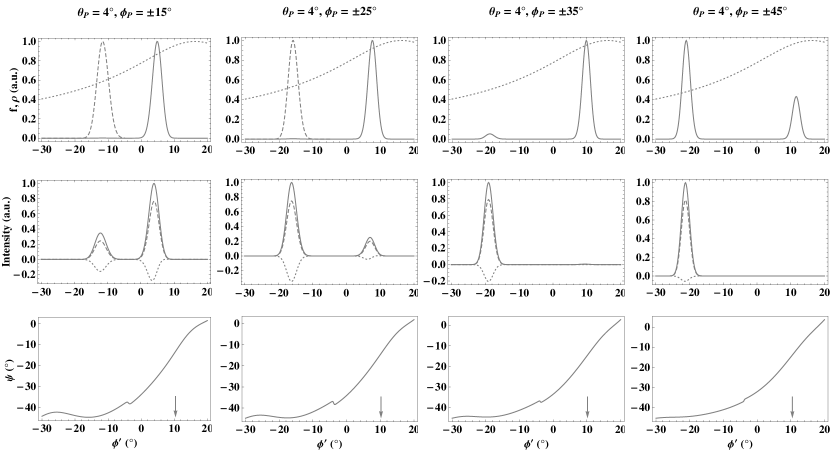
Figure 13: Same as Figure 11 but with two Gaussian modulations symmetrically located in a given conal ring at various azimuth. For simulation we used $\sigma_{\theta}=0.003,$ $\sigma_{\phi}=0.1$ and the rest parameters are the same as in Figure 11. The dashed line curves in the first two columns of the upper panels represent an amplified $f$ to unity to identify with the corresponding intensity component.

In Figure 13, we presented the simulations for different cases of two Gaussian modulations symmetrically located in a given ring centered on the magnetic axis. Although, the asymmetry in $\rho$ between the leading and trailing sides is same in all the cases with much larger curvature on the leading side, there is a diverse asymmetry in the strength of the intensity component between the leading and trailing sides. This is due to an induced asymmetry in the strength of modulation that the inertial observer encounters between the leading and trailing sides. In the case of $\theta_{P}=4^{\circ}$ and $\phi_{P}=\pm 15^{\circ},$ observer encounters a much weaker modulation on the leading side than that on the trailing side which overcomes the influence of asymmetric $\rho.$ Hence, it results in a stronger trailing side component than that on the leading side. Whereas in the case $\theta_{P}=4^{\circ}$ and $\phi_{P}=\pm 25^{\circ},$ observer encountered asymmetry in the modulation strength between the leading and trailing sides becomes smaller compared to that in the case $\theta_{P}=4^{\circ}$ and $\phi_{P}=\pm 15^{\circ}.$ Hence the leading side intensity component becomes stronger than the trailing one as the influence of asymmetry in $\rho$ becomes much important than that in $f.$ In case of $\theta_{P}=4^{\circ}$ and $\phi_{P}=\pm 35^{\circ},$ the asymmetry in the modulation strength between the leading and trailing sides becomes even smaller, and hence resulted in mostly in leading side component. In case of $\theta_{P}=4^{\circ}$ and $\phi_{P}=\pm 45^{\circ},$ observer encounters higher modulation strength on the leading side than that on trailing side, and hence resulted in a single leading side component or a partial cone.

In all the cases, circular polarization is found to be symmetric type over both the leading and trailing side components due the selective enhancement of negative polarity caused by the rotation and PC–current perturbation. Note that for example in the case of $\theta_{P}=4^{\circ}$ and $\phi_{P}=\pm 15^{\circ},$ the emissions from the region, which is closer to the magnetic axis, are selectively enhanced, and hence a selective enhancement of inner circular occurs (see for e.g., the case $\alpha=10^{\circ}$ and $\sigma=5^{\circ}$ in Figure 10). The kinks are introduced into the PPA swing due to the combined effect of modulation and perturbation caused by rotation and PC–current.

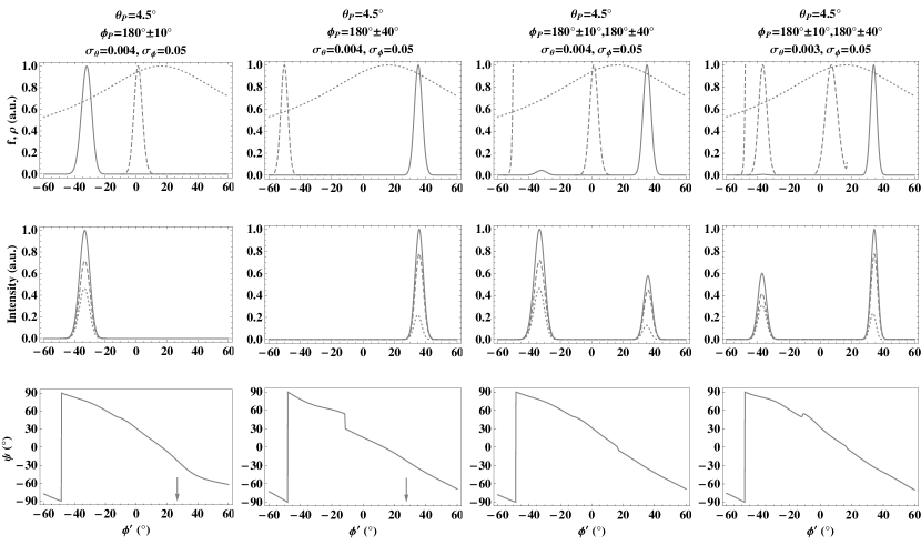
Figure 14: Same as Figure 13 except with $\sigma=-5^{\circ}$ and two Gaussian modulations considered in the first two column panels whereas four Gaussian modulations in the third and last column panels with different modulation parameters.

Similar to Figure 13, we selected Gaussian modulations which are symmetrically located on either sides of the magnetic meridian plane in a given cone, and the simulated profiles are shown in Figure 14 for $\sigma=-5^{\circ}.$ Similar to the cases in Figure 13, the modulation strength that the observer encounters can be quite different between the leading and trailing sides in addition to an asymmetric $\rho.$ Hence it leads to a larger asymmetry in the strength of components between the two sides. In the case $\phi_{P}=180^{\circ}\pm 10^{\circ}$ observer misses out the trailing side modulation and hence only the leading side component shows up, whereas in the case $\phi_{P}=180^{\circ}\pm 40^{\circ}$ it becomes vice versa. For third column, we used the combined modulation that are used in the first two columns (four Gaussian modulations). Even though observer encounters a weaker modulation on the leading side, due to larger curvature on the leading side the component on the leading side becomes stronger than the corresponding one on trailing side. But in the case of last column panels, observer encounters even weaker modulation on the leading side than on the trailing side as compared to the case of third column. Hence the resultant leading side component becomes weaker than the corresponding trailing side one. In all the cases, similar to Figure 13, due to the selective enhancement, the circular polarization becomes positive symmetric type over both the leading and trailing sides.

4 DISCUSSION

The poloidal PC–current perturbs the underlying dipole field by inducing a toroidal magnetic field (Hibschman & Arons, 2001; KG, 2012b) whereas the pulsar rotation causes the bending of trajectory of the field line constrained plasma in the direction of pulsar rotation (e.g., BCW, 1991; Gangadhara, 2005; Thomas & Gangadhara, 2007; Dyks, 2008; Dyks et al., 2010; Thomas et al., 2010; KG, 2012a; Wang et al., 2012). They significantly affect the phase locations of the intensity components as well as the PPA inflection point by introducing an asymmetric phase shifts between them. Rotation (aberration) shifts intensity to the leading side and the PPA inflection point to the trailing side irrespective of sign of $\sigma$ (for e.g., BCW, 1991; Gangadhara, 2005; Thomas & Gangadhara, 2007; Dyks, 2008; Dyks et al., 2010; Thomas et al., 2010; KG, 2012a; Wang et al., 2012). On the other hand PC–current along with modulation can shift the intensity to trailing side and the PPA inflection point to the leading side for the positive $\sigma,$ and vice versa for negative $\sigma$ (KG, 2012b). The influences of the rotation and PC–current adds up for the negative $\sigma$ but cancel each other when $\sigma$ is positive. Note that the opposite behavior of rotation and PC–current in the case of positive $\sigma$ is due to the opposite directions of induced curvature caused by the two perturbations.

Although the effects of rotation and PC–current perturbation can be understand qualitatively when they are combined together, their quantitative estimate becomes impossible when the two effects are considered separately as shown in sections $2$ and $3.$ However, since the influence of rotation is mostly larger than that of the PC–current, in the combined cases mostly the effects of rotation prevail with quite different magnitudes. For example, the phase delay between the PPA inflection point and the central component of pulse profile becomes much smaller for the positive $\sigma$ as compared to that for the negative $\sigma$ (see Figure 6). Hence the above said phase delays greatly depend on the geometric parameters which has not been reported in the literature.

Even though the curvature of source trajectory on the leading side becomes larger than that on the trailing side due to the perturbation caused by the rotation and PC–current considered together, the net modulated intensity can become stronger either on the leading side or on the trailing side (see Figures 13 and 14) depending upon the modulation location and the viewing geometry. Statistically, although there is an observational support for the leading side component dominating over the trailing one, the other contrary cases are also reported (Lyne & Manchester, 1988). Hence our model provides a much plausible explanation for the usual asymmetry between the leading and trailing side components. KG (2012b), by considering the PC–current alone, also have predicted above behavior in the absence of strong rotation effect. However by considering effect of pulsar rotation on the field line constrained plasma alone, BCW (1991) have predicted that the leading side intensity dominate over the trailing side and later Thomas & Gangadhara (2007), Dyks (2008), Dyks et al. (2010), Thomas et al. (2010), KG (2012a), Wang et al. (2012) have arrived at the same conclusion. The “partial cone” pulsars, which show either missing or much suppressed side in their conal double component profiles (Lyne & Manchester, 1988) can be result due to the rotation and PC–current perturbation (see Figures 13 and 14).

Further the rotation and PC-current perturbation introduce an asymmetry into the width of components between the leading and trailing sides in such a way that the leading side components become broader than the corresponding trailing ones, and it has an observational support too (Ahmadi & Gangadhara, 2002). This is due to an induced asymmetry in the steepness of radius of curvature with respect to the rotation phase wherein the trailing side $\rho$ becomes more steeper than that on the leading side. KG (2012a) and KG (2012b) have also predicted the same behavior by considering the effects of rotation and PC–current separately.

The rotation and PC–current significantly introduce an asymmetry into the strengths of opposite polarities of the circular polarization. When they are considered separately, they selectively enhance either the negative or positive polarities. Further the two effects cause the emission pattern to rotate in $(\theta,~{}\phi)-$plane in the opposite directions for positive $\sigma$ and in same direction for negative $\sigma.$ Hence it results in smaller rotation of the emission pattern in $(\theta,~{}\phi)-$plane for the positive $\sigma$ case than that for the negative $\sigma.$ However due to the rotation of the emission pattern, the symmetric type circular polarization becomes evident in addition to the more common antisymmetric type with an usual asymmetry between the opposite polarities in presence of nonuniform distribution of sources (see also KG, 2012a, b). Due to perturbations we find the sign reversal of circular polarization from negative to positive near the center of pulse profile can be associated with either the increasing or decreasing PPA swing, and similarly the vice versa (see Figures 11 and 12), and these deductions are found to be in accordance with Han et al. (1998) and You & Han (2006) observational findings.

Our simulations (see Figures 13 and 14) also confirm Han et al. (1998) and You & Han (2006) findings that the negative polarity of the circular polarization is associated with increasing PPA and vice versa for positive polarity on both the sides of conal-double pulsars profiles. This is possible due to combined rotation and PC-current perturbation under specific conditions that when the modulation is more effective in the polar direction than in azimuthal direction. However KG (2012a) have claimed that such correlation can exist provided in addition to the effective modulation in the polar direction, their location must be asymmetric in a given conal ring centered on the magnetic axis.

Some pulsars particularly millisecond pulsars show the polarization angle behavior that deviates from the standard ‘S’ curve (Xilouris et al., 1998). We find that the ‘kinky’ type distortions in PPA profile are due to the superposition of modulated incoherent emissions over the regions which are larger than the wavelength of radiation in presence of strong rotation and PC-current perturbations. Note that Gangadhara (2010) and KG (2012a) also have obtained the similar results. However, the results of Gangadhara (2010) were in the absence of any perturbation and hence the PPA distortions from the standard ‘S’ curve are smaller. Mitra & Seiradakis (2004) have speculated that if the radio emission has a varying emission height across the pulse profile then PPA swing will be nonuniform. Also, in the literature the kinky type origin has been attributed to multi polar magnetic field in the radio emission region (Mitra et al., 2000) and to the return currents in the pulsar magnetosphere (Ramachandran & Kramer, 2003).

Note that we have performed modeling of coherent pulsar radio emission in terms of single particle curvature radiation. Although to the first order it is not a bad assumption, in reality the efficiency of coherence process may depend on many factors and hence there may be an induced asymmetries in the pulsar emission and polarization between the leading and trailing sides. For example the coherent emitters may be brighter on one side of the profile than on the other side depending upon the factors influencing the coherence process. And this can act in the same direction or in opposite direction to the processes that we have considered in this paper.

Note that we have performed modeling of coherent pulsar radio emission in terms of single particle curvature radiation. Although to the first order it is not a bad assumption, in reality the efficiency of coherence process may depend on many factors and hence there may be an induced asymmetries in the pulsar emission and polarization between the leading and trailing sides. For example the coherent emitters may be brighter on one side of the profile than on the other side depending upon the factors influencing the coherence process. And this can act in the same direction or in opposite direction to the processes that we have considered in this paper.

5 CONCLUSION

We believe our model is much more realistic for pulsar emission and polarization than those proposed before, as for the first time it simultaneously takes into account of the perturbation caused jointly by the rotation and the PC–current. In addition it considers the detailed study on nonuniform source distribution (modulation) and the influence of viewing geometry on pulsar emission. Hence we believe one can explain most of the observed emission and polarization properties of pulsars within the frame work of curvature radiation. On the basis of our simulation of pulse profiles we draw the following conclusions:

1. The effect of rotation and PC–current perturbation in the presence of nonuniform source distribution (modulation) along with viewing geometry might be responsible for the most of the observed diverse behavior of polarization properties of pulsar radio emission.

2. Because of the perturbations there arises an asymmetry in the phase shift of intensity components and PPA inflection point for $\pm\sigma.$ Further we notice that the phase delay of the PPA inflection point with respect to that of the central component (core) becomes larger for negative $\sigma$ than that for the positive $\sigma$.

3. The leading side components can become either stronger or weaker than the corresponding trailing side components of a given cone. This is due to the induced asymmetry in the curvature of source trajectory and the sight line encountered asymmetry in the modulation strength between the two sides.

4. Both the “antisymmetric” and “symmetric”$-$types circular polarization are possible within the frame work of curvature radiation when the perturbation and modulation are operative.

5. In the presence of perturbation the sign reversal of the “antisymmetric”$-$type circular polarization as well as the sign of the “symmetric”$-$type circular polarization do not show the correlation with the sign of the PPA swing in the case of central core dominated pulsars.

6. The ‘kinky’ type distortions in the PPA swing could be due to the incoherent addition of modulated emissions in presence of strong perturbations.

References

- Ahmadi & Gangadhara (2002) Ahmadi, P., & Gangadhara, R. T. 2002, ApJ, 566, 365
- BCW (1991) Blaskiewicz, M., Cordes, J. M., & Wasserman, I. 1991, ApJ, 370, 643, (BCW 1991)
- Dyks (2008) Dyks, J. 2008, MNRAS, 391, 859
- Dyks et al. (2004) Dyks, J., Rudak, B., & Harding, A. K. 2004, ApJ, 607, 939
- Dyks et al. (2010) Dyks, J., Wright, G. A. E., & Demorest, P. 2010, MNRAS, 405, 509
- Gangadhara (1997) Gangadhara, R. T. 1997, A&A, 327, 155
- Gangadhara (2005) Gangadhara, R. T. 2005, ApJ, 628, 923
- Gangadhara (2010) Gangadhara, R. T. 2010, ApJ, 710, 29
- Gangadhara & Gupta (2001) Gangadhara, R. T., & Gupta, Y. 2001, ApJ, 555, 31
- Gil & Snakowski (1990a) Gil, J. A., & Snakowski, J. K. 1990a, A&A, 234, 237
- Gil & Snakowski (1990b) Gil, J. A., & Snakowski, J. K. 1990b, A&A, 234, 269
- Gil et al. (1993) Gil, J. A., Kijak, J. & Zycki, P. 1993, A&A, 272, 207
- Gil et al. (2004) Gil, J., Lyubarsky, Y., & Melikidze, G. I. 2004, ApJ, 600, 872
- Gupta & Gangadhara (2003) Gupta, Y., & Gangadhara, R. T. 2003, ApJ, 584, 418
- Han et al. (1998) Han, J. L., Manchester, R. N., Xu, R. X., & Qiao, G. J., 1998, MNRAS, 300, 373
- Hibschman & Arons (2001) Hibschman, J. A., & Arons, J. 2001, ApJ, 546, 382
- Jackson (1998) Jackson, J. D. 1998, Classical Electrodynamics, (New York: Wiley)
- KG (2012a) Kumar, D., & Gangadhara, R. T. 2012a, ApJ, 746, 157, (KG 2012a)
- KG (2012b) Kumar, D., & Gangadhara, R. T. 2012b, ApJ, 754, 55, (KG 2012b)
- Lyne & Manchester (1988) Lyne, A. G., & Manchester, R. N. 1988, MNRAS, 234, 477
- Melikidze et al. (2000) Melikidze, G. I., Gil, J. A., & Pataraya, A. D. 2000, ApJ, 544, 1081
- Michel (1987) Michel, F. C. 1987, ApJ, 322, 822
- Mitra & Deshpande (1999) Mitra, D., & Deshpande, A. A. 1999, A&A, 346, 906
- Mitra et al. (2000) Mitra, D., Konar, S., Bhattacharya, D., Hoensbroech, A. V., Seiradakis, J. H., & Wielebinski, R. 2000, IAU Colloq. 177: Pulsar Astronomy - 2000 and Beyond, 202, 265
- Mitra & Rankin (2002) Mitra, D., & Rankin, J. M. 2002, ApJ, 577, 322
- Mitra & Seiradakis (2004) Mitra, D., & Seiradakis, J. H. 2004, Hellenic Astronomical Society Sixth Astronomical Conference, 205
- Radhakrishnan & Cooke (1969) Radhakrishnan, V., & Cooke, D. J. 1969, Astrophys. Lett., 3, 225
- Radhakrishnan & Rankin (1990) Radhakrishnan, V., & Rankin, J. M. 1990, ApJ, 352, 258
- Ramachandran & Kramer (2003) Ramachandran, R., & Kramer, M. 2003, A&A, 407, 1085
- Rankin (1983) Rankin, J. M. 1983, ApJ, 274, 333
- Rankin (1990) Rankin, J. M. 1990, ApJ, 352, 247
- Rankin (1993) Rankin, J. M. 1993, ApJS, 85, 145
- Ruderman & Sutherland (1975) Ruderman, M. A., & Sutherland, P. G. 1975, ApJ, 196, 51
- Sturrock (1971) Sturrock, P. A. 1971, ApJ, 164, 229
- Thomas & Gangadhara (2007) Thomas, R. M. C., & Gangadhara, R. T. 2007, A&A, 467, 911
- Thomas & Gangadhara (2010) Thomas, R. M. C., & Gangadhara, R. T. 2010, A&A, 515, 86
- Thomas et al. (2010) Thomas, R. M. C., Gupta, Y., & Gangadhara, R. T. 2010, MNRAS, 406, 1029
- Wang et al. (2012) Wang, P. F., Wang, C., & Han, J. L. 2012, MNRAS, 423, 2464
- Xilouris et al. (1998) Xilouris, K. M., Kramer, M., Jessner, A., et al. 1998, ApJ, 501, 286
- You & Han (2006) You, X. P., & Han, J. L. 2006, Chin. J. Astron. Astrophys., 6, 237