Temporal decorrelations in compressible isotropic turbulence

Abstract

Temporal decorrelations in compressible isotropic turbulence are studied using the space-time correlation theory and direct numerical simulation. A swept-wave model is developed for dilatational components while the classic random sweeping model is proposed for solenoidal components. The swept-wave model shows that the temporal decorrelations in dilatational fluctuations are dominated by two physical processes: random sweeping and wave propagation. These models are supported by the direct numerical simulation of compressible isotropic turbulence, in the sense of that all curves of normalized time correlations for different wavenumbers collapse into a single one using the normalized time separations. The swept-wave model is further extended to account for a constant mean velocity.

A milestone in isotropic and homogeneous turbulence is the random sweeping hypothesis Kraichnan (1964); Tennekes (1975). The random sweeping hypothesis proposes that there is a temporal decorrelation process in incompressible isotropic turbulence and develops a simple model for space-time correlations of velocity fluctuations Kraichnan (1964). These results are examined theoretically Yakhot et al. (1989); Chen and Kraichnain (1989); Nelkin and Tabor (1990) and verified experimentally Praskovsky et al. (1993) and numerically Sanada and Shanmugasundaram (1992); He et al. (2004). The space-time correlation models are used to predict the scalings of wavenumber or frequency energy spectra in turbulent flows Rubinstein and Zhou (1999); Sagaut and Cambon (2008). The decorrelation processes are also relevant to the non-Gaussian statistics Kaneda et al. (1999) and intermittency Tsinober et al. (2001). Their further applications can be found in turbulence generated noise Wang et al. (2006). The recently increasing studies on compressible isotropic turbulence raise such a question on the effects of compressibility on decorrelation processes Benzi et al. (2008); Pan et al. (2009); Aluie (2011). In this letter, we will study the decorrelation processes in compressible isotropic turbulence and propose a model for space-time correlations of dilatational components.

A compressible turbulence is associated with two characteristic velocities: fluid velocity and sound speed, whereas an incompressible one is only associated with fluid velocity. Therefore, the decorrelation processes in compressible turbulence are very different from incompressible one. A space-time correlation is the essential quantity to measure the decorrelation processes in turbulent flows. Three typical models exist for space-time correlations in turbulence theory. The first one is, as stated above, the random sweeping model for incompressible turbulence Kraichnan (1964). We will show that it cannot characterize the acoustic components in compressible turbulence. The second one is the Taylor frozen flow model Taylor (1938). It has been shown that this model is not a good approximation for dilatational components Lee et al. (1992). The third one is the linear wave propagation model Lee et al. (1992). This model can be used for dilatational components if compressible turbulence has a dominating mean velocity. However, we will find that it does not decrease with increasing temporal separation, which violates the nature of correlation functions.

In the present letter, we will develop a space-time correlation model for compressible isotropic turbulence. This is achieved by the Helmholtz decomposition: a velocity field can be split into the solenoidal and dilatational components. A swept-wave model will be developed for the dilatational components while the solenoidal components are expected to follow the random sweeping model. The swept-wave model will be numerically validated and further used to elucidate the decorrelation process in compressible turbulence.

We consider compressible and isotropic turbulence with periodic boundary conditions. In this case, the Helmholtz decomposition for velocity fields can be made as follows Sagaut and Cambon (2008)

$${\bf u}={\bf u}^{s}+{\bf u}^{d},$$ (1)

where ${\bf u}^{s}$ and ${\bf u}^{d}$ are the solenoidal (i.e. incompressible) and dilatational components, respectively. The harmonic component is taken to be zero. We will investigate the temporal decorrelations of solenoidal and dilatational components. The temporal decorrelations can be measured by the space-time correlations of velocity fluctuations

$$R(r,\tau)=\langle u_{\ell}({\bf x},t)u_{\ell}({\bf x}+{\bf r},t+\tau)\rangle,$$ (2)

or its equivalent forms in Fourier space

$${\hat{R}}(k,\tau)=\langle\hat{u}_{\ell}({\bf k},t)\hat{u}_{\ell}(-{\bf k},t+\tau)\rangle.$$ (3)

Here, r and k are the magnitudes of separation vector ${\bf r}$ and wavenumber vector ${\bf k}$. The similar quantities $R^{s}$ and $R^{d}$ can be defined for the solenoidal and dilatational components ${\bf u}^{s}$ and ${\bf u}^{d}$, respectively.

We propose that a solenoidal component follows the same decorrelation process as the random sweeping process for incompressible isotropic turbulence: small eddies are randomly convected or swept by energy-contained eddies, where the contribution of dilatational components to the energy-contained eddies is comparably small Moin (2009). The random sweeping process can be described by a simple idealized convection equation as follows Kraichnan (1964)

$$\left(\frac{\partial}{\partial t}+v_{j}\frac{\partial}{\partial x_{j}}\right)u^{s}_{\ell}=0,$$ (4)

where ${\bf v}=(v_{1},v_{2},v_{3})$ is a spatially uniform and stationary Gaussian random field. $V=|{\bf v}|/\sqrt{3}$ is the r.m.s of solenoidal components along one axis. Its solution in the Fourier space is given by

$$\hat{u}^{s}_{\ell}({\bf k},t)=\hat{u}^{s}_{\ell}({\bf k},0)\exp\left[-i({\bf k\cdot v})t\right].$$ (5)

The time correlation of Fourier mode is formulated as

$${\hat{R}}^{s}(k,\tau)={\hat{R}}^{s}(k,0)\exp\left(-\frac{1}{2}V^{2}k^{2}\tau^{2}\right).$$ (6)

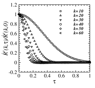
Figure 1: Normalized time correlations of solenoidal components vs time separations for $k=10,20,30,40,50,60$.

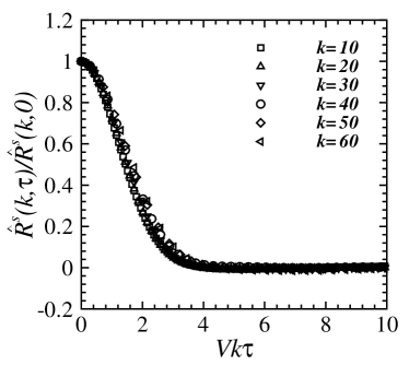
Figure 2: Normalized time correlations of solenoidal components vs normalized time separations $Vk\tau$ for $k=10,20,30,40,50,60$.

A dilatational component in compressible isotropic turbulence propagates at the speed of sound relative to moving fluids. This implies that the dilatational fluctuations are swept by the energy-contained eddies. Therefore, the temporal decorrelations in dilatational components are governed by two dynamic processes: random sweeping and wave propagation. The well-known linear wave propagation model Lee et al. (1992) only includes the wave propagation process. In order to account for the random sweeping effect, we introduce a new term ${\bf v\nabla}$ into the linear wave propagation equation and propose the governing equation for dilatational fluctuations as follows

$$\left(\frac{D^{2}}{Dt^{2}}-\bar{a}^{2}\nabla^{2}\right)u^{d}_{\ell}=0,$$ (7)

where ${\bar{a}}$ is the mean speed of sound and

$$\frac{D}{Dt}=\left(\frac{\partial}{\partial t}+{\bf v}\cdot\nabla\right)=\left(\frac{\partial}{\partial t}+v_{j}\frac{\partial}{\partial x_{j}}\right).$$ (8)

Here, ${\bf v}$ is the same Gaussian random field as one in Eq. (4). The new term ${\bf v\nabla}$ in Eq. (7) represents the random sweeping effect, which is absent in the linear wave propagation model Lee et al. (1992). The solution of Eq. (7) in Fourier space is given by

$$\hat{u}^{d}_{\ell}({\bf k},t) = \hat{u}^{d+}_{\ell}({\bf k},0)\exp\left[-i({\bf k\cdot v})t-ik\bar{a}t\right]+$$ (9)

$$\hat{u}^{d-}_{\ell}({\bf k},0)\exp\left[-i({\bf k\cdot v})t+ik\bar{a}t\right],$$

where $\hat{u}^{d+}_{\ell}$ and $\hat{u}^{d-}_{\ell}$ are the Fourier coefficients.

The time correlation of Fourier mode is calculated as follows

$${\hat{R}}^{d}(k,\tau) = \langle\hat{u}^{d}_{\ell}({\bf k},t)\hat{u}^{d}_{\ell}(-{\bf k},t+\tau)\rangle$$

$$= \langle\hat{u}^{d+}_{\ell}({\bf k},0)\hat{u}^{d+}_{\ell}(-{\bf{k}},0)\rangle\langle\exp[{i({\bf k\cdot v})\tau}+ik\bar{a}\tau]\rangle$$

$$+ \langle\hat{u}^{d-}_{\ell}({\bf k},0)\hat{u}^{d-}_{\ell}(-{\bf{k}},0)\rangle\langle\exp[{i({\bf k\cdot v})\tau}-ik\bar{a}\tau]\rangle.$$

Here, the mode correlation $R^{d}(k,0)$ is given by

$$\frac{1}{2}{\hat{R}}^{d}(k,0)=\langle{\hat{u}^{d+}_{\ell}(-\mathbf{k},0)\hat{u}^{d+}_{\ell}(\mathbf{k},0)}\rangle=\langle{\hat{u}^{d-}_{\ell}(-\mathbf{k},0)\hat{u}^{d-}_{\ell}(\mathbf{k},0)}\rangle.$$

Therefore, the correlation functions can be expressed as

$$\frac{{\hat{R}}^{d}(k,\tau)}{{\hat{R}}^{d}(k,0)}=\cos(k\bar{a}\tau)\exp\left[-\frac{1}{2}k^{2}V^{2}\tau^{2}\right].$$ (11)

The swept-wave model (11) contains two factors: a linear wave function and an exponential function. The first factor represents the random sweeping effect and the second one represents the wave propagation process. If the sweeping velocity is zero, it becomes the linear wave propagation model. In fact, the linear wave propagation model in compressible isotropic turbulence is simplified as $\cos(k\bar{a}\tau)$, which is the inverse Fourier transformation of Equation (19) in Lee et al. (1992). This cosine function does not decay to zero as time separation increases.

To validate the swept-wave model, we solve the three-dimensional, compressible Navier-Stokes equations in a cubic box of side $2\pi$ with specific heat ratio $\gamma=1.4$ and Prandtl number $Pr=0.7$ using an optimized sixth order compact, finite difference scheme. Statistically stationary flow fields are achieved by including a forcing term $\mathbf{f}(\mathbf{x},t)$ with solenoidal modes only, $\nabla\cdot\mathbf{f}=0$. The forcing term is nonzero only in the range $1\leq k\leq 3$ and obeys a Gaussian random distribution with an exponential temporal correlation. Each component of $\mathbf{\hat{f}}(\mathbf{k},t)$ is defined by $\hat{f}_{i}=(\delta_{ij}-k_{i}k_{j}/k^{2})\hat{g}_{j}$, where $\hat{g}_{j}$ is generated by an independent Uhlenbeck-Ornstien process. After the flow fields become statistically stationary, a total of 400 flow fields with computational time increment $0.02$ are chosen to calculate time correlations. The Taylor’s micro-scale based Reynolds number is about 80 and the turbulent Mach number is about 0.63. We also compare the space-time correlations from the present case with ones from decaying turbulence. The results obtained are consistent.

Fig. 1 shows the correlation coefficients of solenoidal modes for wavenumbers $k=10,20,\cdots$ $50$ and $60$, spanning a range of scales from the integral scale to the dissipation scales. The correlation coefficients are the normalized correlation functions by the mode correlation ${\hat{R}}^{s}(k,0)$. Obviously, the solenoidal modes decorrelate more quickly at larger wavenumbers than at small wavenumbers. These results in Fig. 1 are all plotted together in Fig. 2, with the horizontal axis defined by the normalized time scale $Vk\tau$. This normalization causes excellent collapse of the correlation coefficients. The collapse on the normalized time scale $Vk\tau$ supports the random sweeping hypothesis for the solenoidal components.

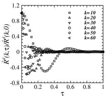
Figure 3: Normalized time correlations of dilatational components vs time separations for $k=10,20,30,40,50,60$.

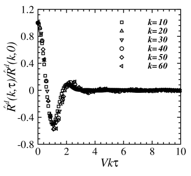
Figure 4: Normalized time correlations of dilatational components vs normalized time separations $Vk\tau$ for $k=10,20,30,40,50,60$.

Fig. 3 plots the normalized time correlations ${\hat{R}}^{d}(k,\tau)/{\hat{R}}^{d}(k,0)$ for dilatational components from DNS data for wavenumber $k=10,20,\cdots$ and $60$, where the correlations are normalized by the correlation ${\hat{R}}^{d}(k,0)$. It is observed from Fig. 3 that the time correlations of dilatational components decay with oscillations. This is very different from solenoidal components where the time correlations decay without any oscillation. These oscillatory decays confirm that temporal decorrelations in dilatational components are mainly determined by both random sweeping and wave propagation.

Fig. 4 presents the normalized time correlations ${\hat{R}}^{d}(k,\tau)/{\hat{R}}^{d}(k,0)$ versus the normalized time separation $Vk\tau$ for wavenumber $k=10,20,\cdots$, $50$ and $60$. The time normalization leads to the virtual collapse of all curves. The collapsed curves decay with oscillations. This result verifies the proposed swept-wave model for dilatational components. We note that the ratio of two scale-similarity variables $Vk\tau$ and ${\bar{a}}k\tau$ is constant.

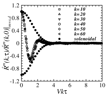
Figure 5: Normalized time correlations vs normalized time separations $Vk\tau$. Dilatational components for $k=10,20,30,40,50,60$; solenoidal component and its mirror image for $k=30$.

Fig. 5 compares the collapsed curves for solenoidal components with the collapsed ones for dilatational components, where the horizontal axis is normalized as the scale-dependent similarity variable $Vk\tau$. It is observed that the collapsed curves for solenoidal components act as an envelop of the collapsed one for dilatational components. This confirms the swept-wave model where the exponential function $\exp(-0.5V^{2}k^{2}\tau^{2})$ acts as an envelop.

We can further calculate the space-time correlations of dilatational components using the Fourier transformation of ${\hat{R}}^{d}(k,\tau)$ from wavenumber space to spatial one

$$R^{d}(r,\tau) = \int_{0}^{\infty}E(k)\exp\left(-\frac{1}{2}V^{2}k^{2}\tau^{2}\right)$$ (12)

$$\cos(k\bar{a}\tau)\frac{\sin(kr)}{kr}dk.$$

Eq. (12) can be extended to account for a constant mean velocity. Without loss of generality, we choose the constant mean velocity $U_{1}$ in the direction of the $x_{1}$ axis. Applying the coordinate transformation $(y_{1}=x_{1}-U_{1}t,y_{2}=x_{2},y_{3}=x_{3})$ to Eq. (7), we obtain

$$R^{d}(r,\tau) = \int_{0}^{\infty}E(k)\mathrm{exp}\left(-\frac{1}{2}V^{2}k^{2}\tau^{2}\right)$$ (13)

$$\cos(k\bar{a}\tau)\frac{\sin\left[k(r-U_{1}\tau)\right]}{k(r-U_{1}\tau)}dk.$$

In comparison with the linear wave propagation model, this model (13) contains an additional exponential function that is responsible for the random sweeping effect. It also confirms that Taylor’s frozen flow model is not a good approximation to the space-time correlation of dilatational components. Wilczek and Narita Wilczek and Narita (2012) consider the random sweeping model with constant mean velocity. The present model is consistent with their results.

In summary, we find that solenoidal and dilatational components in compressible isotropic turbulence display different decorrelation processes: a dilatational component is dominated by both random sweeping and wave propagation while a solenoidal component dominated by the random sweeping effect. We further develop a swept-wave model for dilatational fluctuations. This model is distinct from the linear wave propagation model since it includes the random sweeping process. The DNS data validates the swept-wave model for compressible isotropic turbulence. The further extension of the swept-wave model to turbulent shear flows is referred to the elliptic model Zhao and He (2009) and the present model can be used to study the propagation velocity of coherent structures in compressible turbulence.

Acknowledgements: This work is supported by National Natural Science Foundation of China under projects No. 11232011(Key project) and No. 11021262(Innovative team)and the National Basic Research Program of China (973 Program) under Project No. 2013CB834100 (Nonlinear science).

References

- Kraichnan (1964) R. H. Kraichnan, Phys. Fluids 7, 1723 (1964).
- Tennekes (1975) H. Tennekes, J. Fluid Mech. 67, 561 (1975).
- Yakhot et al. (1989) V. Yakhot, S. A. Orazag, and Z. S. She, Phys. Fluids A 1 (1989).
- Chen and Kraichnain (1989) S. Y. Chen and R. H. Kraichnain, Phys. Fluids A 1 (1989).
- Nelkin and Tabor (1990) M. Nelkin and M. Tabor, Phys. Fluids A 2 (1990).
- Praskovsky et al. (1993) A. A. Praskovsky, E. B. Gledzer, M. Y. Karyakin, and Y. Zhou, J. Fluid Mech. 248, 493 (1993).
- Sanada and Shanmugasundaram (1992) T. Sanada and V. Shanmugasundaram, Phys. Fluids A 4, 1245 (1992).
- He et al. (2004) G. W. He, M. Wang, and S. K. lele, Phys. Fluids 16, 3859 (2004).
- Rubinstein and Zhou (1999) R. Rubinstein and Y. Zhou, Phys. Fluids 11, 2288 (1999).
- Sagaut and Cambon (2008) P. Sagaut and C. Cambon, Homogeneous turbulence dynamics (Cambridge University Press, 2008).
- Kaneda et al. (1999) Y. Kaneda, T. Ishihara, and K. Gotoh, Phys. Fluids 11, 2154 (1999).
- Tsinober et al. (2001) A. Tsinober, P. Vedula, and P. K. Yeung, Phys. Fluids 13, 1974 (2001).
- Wang et al. (2006) M. Wang, J. B. Freund, and S. K. Lele, Annu. Rev. Fluid Mech. 38, 483 (2006).
- Benzi et al. (2008) R. Benzi, L. Biferale, R. T. Fisher, L. P. Kadanoff, D. Q. Lamb, and F. Toschi, Phys. Rev. Lett. 100, 234503 (2008).
- Pan et al. (2009) L. Pan, P. Padoan, and A. G. Kritsuk, Phys. Rev. Lett. 102, 034501 (2009).
- Aluie (2011) H. Aluie, Phys. Rev. Lett. 106, 174502 (2011).
- Taylor (1938) G. I. Taylor, Proc. R. Soc. Lond. A 164, 476 (1938).
- Lee et al. (1992) S. Lee, S. K. Lele, and P. Moin, Phys. Fluids A. 4, 1521 (1992).
- Moin (2009) P. Moin, J. Fluid Mech. 640, 1 (2009).
- Wilczek and Narita (2012) M. Wilczek and Y. Narita, Phys. Rev. E 86, 066308 (2012).
- Zhao and He (2009) X. Zhao and G. W. He, Phys. Rev. E 79, 046316 (2009).