Optimized Transmission with Improper Gaussian Signaling in the $K$-User MISO Interference Channel

Abstract

This paper studies the achievable rate region of the $K$-user Gaussian multiple-input single-output interference channel (MISO-IC) with the interference treated as noise, when improper or circularly asymmetric complex Gaussian signaling is applied. The transmit optimization with improper Gaussian signaling involves not only the signal covariance matrix as in the conventional proper or circularly symmetric Gaussian signaling, but also the signal pseudo-covariance matrix, which is conventionally set to zero in proper Gaussian signaling. By exploiting the separable rate expression with improper Gaussian signaling, we propose a separate transmit covariance and pseudo-covariance optimization algorithm, which is guaranteed to improve the users’ achievable rates over the conventional proper Gaussian signaling. In particular, for the pseudo-covariance optimization, we establish the optimality of rank-1 pseudo-covariance matrices, given the optimal rank-1 transmit covariance matrices for achieving the Pareto boundary of the rate region. Based on this result, we are able to greatly reduce the number of variables in the pseudo-covariance optimization problem and thereby develop an efficient solution by applying the celebrated semidefinite relaxation (SDR) technique. Finally, we extend the result to the Gaussian MISO broadcast channel (MISO-BC) with improper Gaussian signaling or so-called widely linear transmit precoding.

I Introduction

The interference channel (IC) models the practical scenario in wireless communication when more than one transmitter-receiver pairs communicate independent messages simultaneously over the same frequency and thus interfere with each other. Characterizing the information-theoretic capacity for the general $K$-user IC is a long-standing open problem [1]. Moreover, since the capacity-approaching scheme in general requires multi-user encoding and decoding, which are difficult to implement in practical systems, a great deal of research on Gaussian ICs has focused on characterizing the achievable rate regions, under the assumption of employing single-user decoding (SUD) at receivers with the interference treated as noise. Among others, the achievable rate region has been characterized for the Gaussian single-input single-output IC (SISO-IC) [2], single-input multiple-output IC (SIMO-IC) [3], and multiple-input single-output IC (MISO-IC) [4, 5, 6, 7]. In general, the achievable rate region of an IC is completely characterized by its Pareto boundary, which constitutes all the achievable rate-tuples for all users at each of which it is impossible to improve one user’s rate without simultaneously decreasing the rate of at least one of the other users. One approach for such characterization is via solving a sequence of weighted-sum-rate maximization (WSRMax) problems. An alternative method based on the concept of “rate profile” was also proposed in [5] under the MISO-IC setup, which eventually results in solving a sequence of signal-to-interference-plus-noise ratio (SINR) feasibility problems that are easier to handle than WSRMax problems. It is worth mentioning that for the MISO-IC, it has been shown by various methods in [5, 6, 7] that all the rate-tuples on the Pareto boundary can be achieved with transmit beamforming, i.e., with rank-1 transmit covariance matrices.

Besides the achievable rate region characterization, significant research effort on Gaussian ICs has been devoted to solving the WSRMax problems [3, 8, 9, 10, 11, 12, 13, 14, 15, 16, 17]. Unfortunately, such problems have been shown to be NP-hard in general [9]. Many suboptimal algorithms have thus been proposed, e.g., the gradient descent algorithm [10], the interference-pricing based algorithm [11], the game-theory based algorithm [12], and the iterative weighted minimum mean-square-error (MMSE) based algorithm [13]. More recently, for Gaussian SISO-IC, SIMO-IC and MISO-IC, the globally optimal solutions to WSRMax problems have been obtained under the monotonic optimization framework [14, 15, 3, 16, 17]. However, the complexity of such globally optimal algorithms increases exponentially with the number of users, and their extension to the more general multiple-input multiple-output IC (MIMO-IC) still remains unknown. Moreover, it is worth mentioning that there have been a great deal of research interests over the last few years in characterizing Gaussian ICs from the degrees-of-freedom (DoF) perspective using the technique of interference alignment (IA) (see [18] and the references therein).

The existing works on ICs have mostly assumed proper or circularly symmetric complex Gaussian (CSCG) signaling for transmitted signals. It is worth noting that the more general improper or circularly asymmetric complex signal processing has been exploited before in various other areas such as widely linear estimation [19], while only recently it was revealed that improper complex Gaussian signaling, jointly applied with the techniques of symbol extension and IA, is able to improve the achievable sum-rate DoF for the three-user Gaussian SISO-IC at the asymptotically high signal-to-noise ratio (SNR) [20]. Later, it was shown that even for the two-user SISO-IC where IA is not applicable, the achievable rate region can still be enlarged with improper Gaussian signaling over the conventional proper Gaussian signaling at finite SNR [21, 22]. Furthermore, it has been shown in our prior work [23] that with improper Gaussian signaling, the user’s achievable rate in the general MIMO-IC can be expressed as the summation of the rate achievable by the conventional proper Gaussian signaling, which depends on the users’ transmit covariance matrices only, and an additional term, which is a function of both the users’ transmit covariance and pseudo-covariance matrices. Such a separable rate structure has been exploited in [23] to optimize the covariance and pseudo-covariance separately so that the obtained improper Gaussian signaling strictly outperforms the conventional proper Gaussian signaling in terms of the achievable rate region. However, the algorithms proposed in [23] are for the two-user SISO-IC and cannot be applied when there are more than two users and/or multiple antennas at the transmitter. This thus motivates our current work that extends the result in [23] to optimize the transmission with improper Gaussian signaling in the more general $K$-user MISO-IC.

Similar to [5], in this paper we apply the rate-profile technique to characterize the achievable rate region of the MISO-IC with the interference treated as Gaussian noise. However, unlike the case with proper Gaussian signaling considered in [5], the optimization problem with improper Gaussian signaling is non-convex and thus difficult to be solved optimally. By adopting the similar separate covariance and pseudo-covariance optimization approach as in [23], we develop an efficient solution for this problem in the MISO-IC case. Specifically, for the pseudo-covariance optimization, we first establish the optimality for rank-1 pseudo-covariance matrices given the optimal rank-1 transmit covariance matrices for achieving the Pareto optimal rates. Moreover, we show that each rank-1 pseudo-covariance matrix is parameterized by one unknown complex scalar. Based on this result, we formulate the original matrix optimization problem to an equivalent vector optimization problem in considerably lower dimensions. We then apply the celebrated semidefinite relaxation (SDR) technique [24] to find an efficient approximate solution for the reformulated problem. It is worth noting that the approach of using SDR for solving non-convex quadratically constrained quadratic programs (QCQPs) has been successfully applied to find high-quality approximate solutions for various problems in communications and signal processing (see [24] and the references therein). For our pseudo-covariance optimization problem under the $K$-user MISO-IC setup, we show that the proposed SDR-based solution is in fact optimal when $K=2$. Finally, we show that the improper Gaussian signaling scheme developed for the MISO-IC can also be applied to the $K$-user MISO broadcast channel (MISO-BC), under the assumption of employing widely linear precoding at the transmitter.

The rest of this paper is organized as follows. Section II presents the MISO-IC model and the problem formulation. Section III develops the separate covariance and pseudo-covariance optimization algorithm for our formulated problem. In Section IV, the proposed improper Gaussian signaling scheme is extended to the MISO-BC with widely linear precoding. Section V presents numerical results. Finally, we conclude the paper in Section VI.

Notations: In this paper, scalars are denoted by italic letters. Boldface lower- and upper-case letters denote vectors and matrices, respectively. For a square matrix $\mathbf{S}$, $\mathrm{Tr}(\mathbf{S})$ denotes the trace. $\mathbf{S}\succeq\mathbf{0}$ and $\mathbf{S}\succ\mathbf{0}$ mean that $\mathbf{S}$ is positive semidefinite and positive definite, respectively. $\mathbb{C}^{M\times N}$ and $\mathbb{R}^{M\times N}$ denote the space of $M\times N$ complex and real matrices, respectively. For an arbitrary matrix $\mathbf{A}$, $\mathbf{A}^{*}$, $\mathbf{A}^{T}$, $\mathbf{A}^{H}$ and $\mathrm{rank}(\mathbf{A})$ represent the complex-conjugate, transpose, Hermitian transpose and rank of $\mathbf{A}$, respectively. The symbol $i$ denotes the imaginary unit, i.e., $i^{2}=-1$. $[\mathbf{v}]_{j}$ denotes the $j$th element of the vector $\mathbf{v}$, while $\|\mathbf{v}\|$ denotes its Euclidean norm. For a complex number $x$, $|x|$ denotes its magnitude. $\mathcal{CN}(\mathbf{x},\mathbf{\Sigma})$ represents the CSCG distribution of a random vector (RV) with mean $\mathbf{x}$ and covariance matrix $\mathbf{\Sigma}$. $\Re\{\cdot\}$ and $\Im\{\cdot\}$ represent the real and imaginary parts of a complex number, respectively. Finally, $\log(\cdot)$ denotes the logarithm function with base $2$.

II System Model and Problem Formulation

We consider a $K$-user MISO-IC, where each transmitter is intended to send independent information to its corresponding receiver, while possibly interfering with all other $K-1$ receivers. Assume that each transmitter is equipped with $M>1$ antennas and each receiver with one antenna. The received baseband signal for user $k$ is given by

$$y_{k}(n)=\mathbf{h}_{kk}\mathbf{x}_{k}(n)+\sum_{j\neq k}\mathbf{h}_{kj}\mathbf{x}_{j}(n)+v_{k}(n),\ \forall k,$$ (1)

where $n$ is the symbol index; $\mathbf{h}_{kk}\in\mathbb{C}^{1\times M}$ denotes the direct channel from transmitter $k$ to receiver $k$, while $\mathbf{h}_{kj}\in\mathbb{C}^{1\times M},j\neq k$, denotes the interference channel from transmitter $j$ to receiver $k$; we assume quasi-static fading and thus all channels are constant over $n$’s for the case of our interest; $v_{k}(n)$ represents the independent and identically distributed (i.i.d.) zero-mean CSCG noise with variance $\sigma^{2}$, i.e., $v_{k}(n)\sim\mathcal{CN}(0,\sigma^{2})$; and $\mathbf{x}_{k}(n)\in\mathbb{C}^{M\times 1}$ is the transmitted signal vector from transmitter $k$, which is independent of $\mathbf{x}_{j}(n)$ for $j\neq k$. In this paper, for the purpose of exposition, we assume that the technique of symbol extensions over time [20] is not used. Hence, $\mathbf{x}_{k}(n)$ is independent over $n$. For brevity, $n$ is omitted in the rest of this paper. Different from the conventional schemes where proper Gaussian signaling is assumed, i.e., $\mathbf{x}_{k}\sim\mathcal{CN}(\mathbf{0},\mathbf{C}_{\mathbf{x}_{k}})$, with $\mathbf{C}_{\mathbf{x}_{k}}$ denoting the transmit covariance matrix, in this paper, we consider the more general improper Gaussian transmitted signals. For the background knowledge of improper (Gaussian) RVs, the readers may refer to [23, 27] and the references therein.

For the zero-mean transmitted Gaussian RV $\mathbf{x}_{k}$, we denote its covariance and pseudo-covariance matrices as $\mathbf{C}_{\mathbf{x}_{k}}$ and $\widetilde{\mathbf{C}}_{\mathbf{x}_{k}}$, respectively, i.e.,

$$\mathbf{C}_{\mathbf{x}_{k}}=\mathbb{E}(\mathbf{x}_{k}\mathbf{x}_{k}^{H}),\ \widetilde{\mathbf{C}}_{\mathbf{x}_{k}}=\mathbb{E}(\mathbf{x}_{k}\mathbf{x}_{k}^{T}),$$ (2)

where $\mathbf{C}_{\mathbf{x}_{k}}$ is Hermitian and positive semidefinite, and $\widetilde{\mathbf{C}}_{\mathbf{x}_{k}}$ is symmetric in general. For the conventional proper Gaussian signaling, the pseudo-covariance matrices $\widetilde{\mathbf{C}}_{\mathbf{x}_{k}}$’s for all transmitters are set to zero matrices, and thus are not included in the transmit optimization. However, for the more general improper Gaussian signaling considered in this paper, the additional degrees of freedom given by the pseudo-covariance matrices provide a further opportunity for improving rate over proper Gaussian signaling [18]. $\mathbf{C}_{\mathbf{x}_{k}}$ and $\widetilde{\mathbf{C}}_{\mathbf{x}_{k}}$ are a valid pair of covariance and pseudo-covariance matrices, i.e., there exists a RV $\mathbf{x}_{k}$ with covariance and pseudo-covariance matrices given by $\mathbf{C}_{\mathbf{x}_{k}}$ and $\widetilde{\mathbf{C}}_{\mathbf{x}_{k}}$, respectively, if and only if the corresponding augmented covariance matrix $\underline{\mathbf{C}}_{\mathbf{\mathbf{x}}_{k}}$ defined below is positive semidefinite [28],

$$\underline{\mathbf{C}}_{\mathbf{\mathbf{x}}_{k}}\triangleq\bigg{[}\begin{matrix}\mathbf{C}_{\mathbf{\mathbf{x}_{k}}}&\widetilde{\mathbf{C}}_{\mathbf{x}_{k}}\\ \widetilde{\mathbf{C}}_{\mathbf{x}_{k}}^{*}&\mathbf{C}_{\mathbf{x}_{k}}^{*}\end{matrix}\bigg{]}\succeq\mathbf{0}.$$ (3)

For the MISO-IC, the covariance and pseudo-covariance of the received signal $y_{k}$ can be written as

$$C_{y_{k}} =\mathbb{E}(y_{k}y_{k}^{*})=\sum_{j=1}^{K}\mathbf{h}_{kj}\mathbf{C}_{\mathbf{x}_{j}}\mathbf{h}_{kj}^{H}+\sigma^{2},$$ (4)

$$\widetilde{C}_{y_{k}} =\mathbb{E}(y_{k}y_{k})=\sum_{j=1}^{K}\mathbf{h}_{kj}\widetilde{\mathbf{C}}_{\mathbf{x}_{j}}\mathbf{h}_{kj}^{T}.$$ (5)

It can be seen that $C_{y_{k}}$ is a positive real number whose value equals to the total received power at receiver $k$. Denote the interference-plus-noise term at receiver $k$ as $s_{k}$, i.e., $s_{k}=\sum_{j\neq k}\mathbf{h}_{kj}\mathbf{x}_{j}+v_{k}.$ Then the covariance and pseudo-covariance of $s_{k}$ are given by

$$C_{s_{k}} =\mathbb{E}(s_{k}s_{k}^{*})=\sum_{j\neq k}\mathbf{h}_{kj}\mathbf{C}_{\mathbf{x}_{j}}\mathbf{h}_{kj}^{H}+\sigma^{2},$$ (6)

$$\widetilde{C}_{s_{k}} =\mathbb{E}(s_{k}s_{k})=\sum_{j\neq k}\mathbf{h}_{kj}\widetilde{\mathbf{C}}_{\mathbf{x}_{j}}\mathbf{h}_{kj}^{T}.$$ (7)

With improper Gaussian signaling at all transmitters, the resulting interference at each receiver is improper Gaussian as well. Under the assumption that the improper Gaussian interference is treated as additional noise over existing proper Gaussian background noise at all receivers, an achievable rate expression has been derived in [23] for the $K$-user MIMO-IC. By applying the result in [23] to the MISO-IC setup, the achievable rate of user $k$ can be expressed as

$$R_{k} =\underbrace{\mathrm{log}\left(1+\frac{\mathbf{h}_{kk}\mathbf{C}_{\mathbf{x}_{k}}\mathbf{h}_{kk}^{H}}{\sigma^{2}+\sum_{j\neq k}\mathbf{h}_{kj}\mathbf{C}_{\mathbf{x}_{j}}\mathbf{h}_{kj}^{H}}\right)}_{\triangleq R_{k}^{\text{proper}}(\{\mathbf{C}_{\mathbf{x}_{j}}\})}$$

$$\qquad\qquad\qquad\qquad\qquad+\frac{1}{2}\mathrm{log}\frac{1-C_{y_{k}}^{-2}|\widetilde{C}_{y_{k}}|^{2}}{1-C_{s_{k}}^{-2}|\widetilde{C}_{s_{k}}|^{2}}.$$ (8)

It is observed from (8) that with improper Gaussian signaling, each user’s achievable rate is a summation of the rate achievable by the conventional proper Gaussian signaling, denoted by $R_{k}^{\text{proper}}(\{\mathbf{C}_{\mathbf{x}_{j}}\})$, and an additional term, which is a function of both the users’ covariance and pseudo-covariance matrices. Therefore, for a given set of transmit covariance matrices obtained by any proper Gaussian signaling scheme, the achievable rates in MISO-IC can be improved with improper Gaussian signaling by choosing the pseudo-covariance matrices that make the second term in (8) strictly positive.

Remark 1.

From user $k$’s perspective, with improper Gaussian signaling employed by other transmitters and under the assumption that the resulting interference is treated as additional noise over existing proper or CSCG background noise at the receiver, user $k$ essentially communicates over a point-to-point MISO channel corrupted by improper or circularly asymmetric complex Gaussian noise. Therefore, the well-known result that proper Gaussian signaling is optimal [29], which is applicable for point-to-point channels with proper or CSCG noise only, does not apply here. This thus motivates our work on investigating the more general improper Gaussian signaling for MISO-IC.

The achievable rate region $\mathcal{R}$ for the $K$-user MISO-IC is defined as the set of rate-tuples that can be simultaneously achieved by all users under a given set of transmit power constraints at each transmitter, denoted by $P_{k},k=1,\cdots,K$. With $R_{k}$ given in (8), we thus have

$$\mathcal{R}\triangleq\bigcup_{\begin{subarray}{l}\mathrm{Tr}(\mathbf{C}_{\mathbf{x}_{k}})\leq P_{k},\\ \underline{\mathbf{C}}_{\mathbf{x}_{k}}\succeq\mathbf{0},\ \forall k\end{subarray}}\bigg{\{}(r_{1},\cdots,r_{K}):0\leq r_{k}\leq R_{k},\forall k\bigg{\}},$$ (9)

where the constraint $\underline{\mathbf{C}}_{\mathbf{x}_{k}}\succeq\mathbf{0}$ follows from (3).

To characterize the Pareto boundary of the achievable rate region $\mathcal{R}$, we adopt the rate-profile method as in [5]. Specifically, any Pareto-optimal rate-tuple on the boundary can be obtained by solving the following optimization problem with a given rate-profile vector denoted by $\alpha$$=(\alpha_{1}\cdots\alpha_{K})$.

(P1): $$\underset{\{\mathbf{C}_{\mathbf{x}_{k}}\},\{\widetilde{\mathbf{C}}_{\mathbf{x}_{k}}\},R}{{\mathrm{max.}}}R$$

$$\qquad\ \text{s.t.}\quad R_{k}\geq\alpha_{k}R,\ \forall k,$$

$$\qquad\qquad\ \ \mathrm{Tr}(\mathbf{C}_{\mathbf{x}_{k}})\leq P_{k},\ \forall k,$$

$$\qquad\qquad\ \ \bigg{[}\begin{matrix}\mathbf{C}_{\mathbf{x}_{k}}&\widetilde{\mathbf{C}}_{\mathbf{x}_{k}}\\ \widetilde{\mathbf{C}}_{\mathbf{x}_{k}}^{*}&\mathbf{C}_{\mathbf{x}_{k}}^{*}\end{matrix}\bigg{]}\succeq\mathbf{0},\ \forall k,$$

where $\alpha_{k}$ denotes the target ratio between user $k$’s achievable rate and the users’ sum-rate, $R$. Without loss of generality, we assume $\alpha_{k}>0,\forall k$, and $\sum_{k=1}^{K}\alpha_{k}=1$. Denote the optimal value of (P1) as $R^{\star}$. Then the rate-tuple $R^{\star}\cdot$ $\alpha$ must be on the Pareto boundary of the rate region $\mathcal{R}$. Thereby, by solving (P1) with different rate-profile vectors $\alpha$, the complete Pareto boundary of $\mathcal{R}$ can be found.

III Separate Covariance and Pseudo-Covariance Optimization

(P1) is a non-convex optimization problem, and thus it is difficult to achieve its global optimum efficiently. In this section, we propose a separate covariance and pseudo-covariance optimization algorithm by utilizing the separable rate expression given in (8) to obtain an efficient suboptimal solution for (P1). Specifically, the covariance matrices of the transmitted signals are first optimized by setting the pseudo-covariance matrices to zero, i.e., proper Gaussian signaling is applied. Then, the pseudo-covariance matrices are optimized with the covariance matrices fixed as the previously obtained solution. With such a separate optimization approach, the obtained improper Gaussian signaling design is guaranteed to improve the achievable rates over the conventional proper Gaussian signaling.

III-A Covariance Optimization

When restricted to proper Gaussian signaling by setting $\widetilde{\mathbf{C}}_{\mathbf{x}_{k}}=\mathbf{0},\forall k$, the second term in (8) vanishes to zero and (P1) reduces to

(P1.1): $$\underset{r,\{\mathbf{C}_{\mathbf{x}_{k}}\}}{{\mathrm{max.}}}\ r$$

$$\quad\text{s.t.}\ \mathrm{log}\left(1+\frac{\mathbf{h}_{kk}\mathbf{C}_{\mathbf{x}_{k}}\mathbf{h}_{kk}^{H}}{\sigma^{2}+\sum_{j\neq k}\mathbf{h}_{kj}\mathbf{C}_{\mathbf{x}_{j}}\mathbf{h}_{kj}^{H}}\right)\geq\alpha_{k}r,\ \forall k,$$

$$\qquad\ \ \mathrm{Tr}(\mathbf{C}_{\mathbf{x}_{k}})\leq P_{k},\ \forall k,$$

$$\qquad\ \ \mathbf{C}_{\mathbf{x}_{k}}\succeq\mathbf{0},\ \forall k.$$

Denote the optimal value of (P1.1) as $r^{\star}$. Then the rate-tuple $r^{\star}\cdot\bm{\alpha}$ is on the Pareto boundary of the achievable rate region with proper Gaussian signaling. It has been shown in [5, 6, 7] that all the Pareto-optimal rate-tuples with proper Gaussian signaling can be achieved by rank-1 transmit covariance matrices or beamforming. Therefore, without loss of optimality for (P1.1), we can let

$$\mathbf{C}_{\mathbf{x}_{k}}=\mathbf{t}_{k}\mathbf{t}_{k}^{H},\ \forall k,$$ (10)

where $\mathbf{t}_{k}$ is the transmit beamforming vector for user $k$. Then for any fixed target rate $r$, the feasibility problem related to (P1.1) can be formulated as

(P1.2): $$\text{Find}\ \{\mathbf{t}_{k}\}$$

s.t. $$\sigma^{2}+\sum_{j\neq k}|\mathbf{h}_{kj}\mathbf{t}_{j}|^{2}\leq\frac{1}{2^{\alpha_{k}r}-1}(\mathbf{h}_{kk}\mathbf{t}_{k})^{2},\ \forall k,$$

$$\Im\{\mathbf{h}_{kk}\mathbf{t}_{k}\}=0,\ \|\mathbf{t}_{k}\|^{2}\leq P_{k},\ \forall k,$$

where without loss of generality, we have assumed that for each user $k$, $\mathbf{h}_{kk}\mathbf{t}_{k}$ is a nonnegative real number [30]. (P1.2) is a second-order cone programming (SOCP) problem, which can be efficiently solved [31]. If (P1.2) is feasible, then the optimal value of (P1.1) satisfies $r^{\star}\geq r$; otherwise, $r^{\star}<r$. Therefore, (P1.1) can be optimally solved by solving (P1.2) with different values of $r$, and applying a bisection search over $r$ [31].

III-B Pseudo-Covariance Optimization

Denote the optimal solution to (P1.1) as $\{r^{\star},\mathbf{C}_{\mathbf{x}_{k}}^{\star}=\mathbf{t}_{k}\mathbf{t}_{k}^{H}\}$. By fixing the transmit covariance matrices as $\{\mathbf{C}_{\mathbf{x}_{k}}^{\star}=\mathbf{t}_{k}\mathbf{t}_{k}^{H}\}$, (P1) is further optimized over the pseudo-covariance matrices $\{\widetilde{\mathbf{C}}_{\mathbf{x}_{k}}\}$ in this subsection. By replacing the first term in the rate expression (8) by $\alpha_{k}r^{\star}$, the problem for pseudo-covariance matrix optimization is formulated as

$$\text{(P1.3):}\ \underset{R,\{\widetilde{\mathbf{C}}_{\mathbf{x}_{k}}\}}{\mathrm{max.}} \quad R$$

s.t. $$\alpha_{k}r^{\star}+\frac{1}{2}\mathrm{log}\frac{1-C_{y_{k}}^{-2}|\widetilde{C}_{y_{k}}|^{2}}{1-C_{s_{k}}^{-2}|\widetilde{C}_{s_{k}}|^{2}}\geq\alpha_{k}R,\ \forall k,$$

$$\bigg{[}\begin{matrix}\mathbf{t}_{k}\mathbf{t}_{k}^{H}&\widetilde{\mathbf{C}}_{\mathbf{x}_{k}}\\ \widetilde{\mathbf{C}}_{\mathbf{x}_{k}}^{*}&(\mathbf{t}_{k}\mathbf{t}_{k}^{H})^{*}\end{matrix}\bigg{]}\succeq\mathbf{0},\ \forall k,$$ (11)

where $C_{y_{k}}$ and $C_{s_{k}}$ are fixed covariances given the previously optimized transmit covariance matrices $\{\mathbf{C}_{\mathbf{x}_{k}}^{\star}=\mathbf{t}_{k}\mathbf{t}_{k}^{H}\}$; $\widetilde{C}_{y_{k}}$ and $\widetilde{C}_{s_{k}}$ are the pseudo-covariances, which are related to transmit pseudo-covariance matrices $\{\widetilde{\mathbf{C}}_{\mathbf{x}_{k}}\}$ via (5) and (7), respectively. By treating $R$ as a slack variable and discarding irrelevant terms in (P1.3), the problem can be re-written as a minimum-weighted-rate maximization (MinWR-Max) problem as follows.

$$\text{(P1.4):}\ \underset{\{\widetilde{\mathbf{C}}_{\mathbf{x}_{k}}\}}{\mathrm{max.}}\ \underset{k=1,\cdots,K}{\mathrm{min.}}\ \frac{1}{2\alpha_{k}}\mathrm{log}\frac{1-C_{y_{k}}^{-2}|\widetilde{C}_{y_{k}}|^{2}}{1-C_{s_{k}}^{-2}|\widetilde{C}_{s_{k}}|^{2}}\$$

s.t. $$\bigg{[}\begin{matrix}\mathbf{t}_{k}\mathbf{t}_{k}^{H}&\widetilde{\mathbf{C}}_{\mathbf{x}_{k}}\\ \widetilde{\mathbf{C}}_{\mathbf{x}_{k}}^{*}&(\mathbf{t}_{k}\mathbf{t}_{k}^{H})^{*}\end{matrix}\bigg{]}\succeq\mathbf{0},\ \forall k.$$ (12)

(P1.4) is a matrix optimization problem that deals with the additional rate term in (8) due to the use of improper Gaussian signaling. Denote the optimal value of (P1.4) as $\tau^{\star}$. If $\tau^{\star}>0$, then a strict rate improvement corresponding to rate-profile $\bm{\alpha}$ over the optimal proper Gaussian signaling is achieved. The following result will be used for solving (P1.4).

Lemma 1.

The positive semidefinite constraint in (12) is satisfied if and only if

$$\widetilde{\mathbf{C}}_{\mathbf{x}_{k}}=Z_{k}\widetilde{\mathbf{t}}_{k}\widetilde{\mathbf{t}}_{k}^{T},\ \forall k,$$ (13)

where $Z_{k}$ is a complex scalar variable satisfying $|Z_{k}|\leq\|\mathbf{t}_{k}\|^{2}$, and $\widetilde{\mathbf{t}}_{k}=\mathbf{t}_{k}/\|\mathbf{t}_{k}\|$ denotes the normalized transmit beamforming vector for user $k$ with proper Gaussian signaling.

Proof:

Please refer to Appendix A. ∎

It is noted that $\widetilde{\mathbf{C}}_{\mathbf{x}_{k}}$ in (13) is a rank-1 symmetric matrix, and thus Lemma 1 establishes the optimality of rank-1 pseudo-covariance matrices in the $K$-user MISO-IC, if the optimal rank-1 transmit covariance matrices are applied. Furthermore, it follows from (13) that each of such rank-1 pseudo-covariance matrices is parameterized by one unknown complex scalar $Z_{k}$. As a result, the problem dimension for pseudo-covariance optimization can be significantly reduced from $KM^{2}$ in the original matrix problem (P1.4) to $K$ by applying Lemma 1, as will be shown next.

By substituting (13) into (5) and (7), we have

$$\widetilde{C}_{y_{k}}=\sum_{j=1}^{K}(\mathbf{h}_{kj}\widetilde{\mathbf{t}}_{j})^{2}Z_{j},\ \widetilde{C}_{s_{k}}=\sum_{j\neq k}(\mathbf{h}_{kj}\widetilde{\mathbf{t}}_{j})^{2}Z_{j},\ \forall k.$$ (14)

Define the following $K$-dimensional complex-valued vectors:

$$\mathbf{z}=\left[\begin{matrix}Z_{1}&\cdots&Z_{K}\end{matrix}\right]^{T},$$

$$\mathbf{m}_{k}=C_{y_{k}}^{-1}\left[\begin{matrix}(\mathbf{h}_{k1}\widetilde{\mathbf{t}}_{1})^{2}&\cdots&(\mathbf{h}_{kK}\widetilde{\mathbf{t}}_{K})^{2}\end{matrix}\right]^{H},$$

$$\mathbf{w}_{k}=C_{s_{k}}^{-1}\left[\begin{matrix}\cdots&(\mathbf{h}_{k(k-1)}\widetilde{\mathbf{t}}_{k-1})^{2}&0&(\mathbf{h}_{k{(k+1)}}\widetilde{\mathbf{t}}_{k+1})^{2}&\cdots\end{matrix}\right]^{H}.$$

Then we have

$$C_{y_{k}}^{-2}\big{|}\widetilde{C}_{y_{k}}\big{|}^{2}=|\mathbf{m}_{k}^{H}\mathbf{z}|^{2},$$ (15)

$$C_{s_{k}}^{-2}\big{|}\widetilde{C}_{s_{k}}\big{|}^{2}=|\mathbf{w}_{k}^{H}\mathbf{z}|^{2}.$$ (16)

Therefore, (P1.4) can be reformulated as

$$\text{(P1.5):}\ \underset{\mathbf{z}\in\mathbb{C}^{K}}{\mathrm{max.}}\ \underset{k=1,\cdots,K}{\mathrm{min.}}\ \frac{1}{2\alpha_{k}}\mathrm{log}\frac{1-|\mathbf{m}_{k}^{H}\mathbf{z}|^{2}}{1-|\mathbf{w}_{k}^{H}\mathbf{z}|^{2}}\$$

s.t. $$|\mathbf{e}_{k}^{T}\mathbf{z}|^{2}\leq\big{\|}\mathbf{t}_{k}\big{\|}^{4},\ \forall k,$$ (17)

where $\mathbf{e}_{k}$ is the $k$th column of a $K\times K$ identity matrix. Note that the constraint in (17) corresponds to the condition $|Z_{k}|\leq\|\mathbf{t}_{k}\|^{2}$ given in Lemma 1. Before solving (P1.5), we first give an intuitive discussion on when it is possible for (P1.5) to have a strictly positive objective value, or in other words, to achieve a strict rate improvement over the optimal proper Gaussian signaling by further optimizing the pseudo-covariance matrices.

Denote the second term of the rate expression in (8) as $\Delta R_{k}$, which is the additional rate gain due to the use of improper Gaussian signaling. With the rank-1 transmit covariance and pseudo-covariance matrices given above, a simple upper bound on $\Delta R_{k}$ in (P1.5) can be obtained as

$$\Delta R_{k} =\frac{1}{2}\mathrm{log}\frac{1-|\mathbf{m}_{k}^{H}\mathbf{z}|^{2}}{1-|\mathbf{w}_{k}^{H}\mathbf{z}|^{2}}$$ (18)

$$\leq\frac{1}{2}\mathrm{log}\frac{1}{1-|\mathbf{w}_{k}^{H}\mathbf{z}|^{2}}$$ (19)

$$\leq-\frac{1}{2}\mathrm{log}\big{(}1-\|\mathbf{w}_{k}\|^{2}\|\mathbf{z}\|^{2}\big{)},$$ (20)

where in order for the upper bound in (20) to be meaningful, $\|\mathbf{w}_{k}\|^{2}$ is assumed to be small enough so that $\|\mathbf{w}_{k}\|^{2}\|\mathbf{z}\|^{2}<1$. Note that $\|\mathbf{w}_{k}\|^{2}=C_{s_{k}}^{-2}\sum_{j\neq k}|\mathbf{h}_{kj}\widetilde{\mathbf{t}}_{j}|^{4}$, which reflects the interference level experienced at receiver $k$ given the beamforming vectors $\{\mathbf{t}_{k}\}$. As $\|\mathbf{w}_{k}\|^{2}\rightarrow 0$, the upper bound in (20) approaches to $0$, which leads to the following remark.

Remark 2.

Improper Gaussian signaling is more advantageous than proper Gaussian signaling in MISO-IC only when there is non-negligible interference among the users. For example, with zero-forcing (ZF) transmit beamforming vectors $\{\mathbf{t}_{j}^{\text{ZF}}\}$, i.e., $\mathbf{h}_{kj}\mathbf{t}_{j}^{\text{ZF}}=0$, $\forall j\neq k$, we have $\|\mathbf{w}_{k}\|^{2}=0$ and thus $\Delta R_{k}=0$, $\forall k$. As a result, no rate improvement can be achieved by further optimizing the pseudo-covariance matrices. This is as expected since ZF transmit beamforming essentially results in $K$ independent point-to-point MISO channels, where proper Gaussian signaling is known to be optimal [29].

For the general $K$-user MISO-IC, ZF transmit beamforming is feasible only when the number of transmit antennas at each transmitter is no smaller than the total number of users, i.e., $M\geq K$. For the general case where the users are interfered by each other with non-ZF transmit beamforming, i.e., $\mathbf{w}_{k}\neq\mathbf{0}$, there is then a potential opportunity to improve the achievable rates over the optimal proper Gaussian signaling by solving the pseudo-covariance optimization problem in (P1.5), as we pursue next.

(P1.5) is a problem of maximizing the minimum of $K$ weighted log-fractions of quadratic functions over $\mathbf{z}$, for which the well-known SDR technique can be applied to find an efficient approximate solution [24]. Let $\mathbf{M}_{k}=\mathbf{m}_{k}\mathbf{m}_{k}^{H}$ and $\mathbf{W}_{k}=\mathbf{w}_{k}\mathbf{w}_{k}^{H},\ \forall k$, and with the identity $\mathbf{x}^{H}\mathbf{A}\mathbf{x}=\mathrm{Tr}(\mathbf{A}\mathbf{x}\mathbf{x}^{H})$, the SDR problem of (P1.5) is formulated as

$$\text{(P1.5-SDR):}\ \underset{\mathbf{Z}\succeq\mathbf{0}}{\mathrm{max.}}\ \underset{k=1,\cdots,K}{\mathrm{min.}}\ \frac{1}{2\alpha_{k}}\mathrm{log}\frac{1-\mathbf{\mathrm{Tr}}(\mathbf{M}_{k}\mathbf{Z})}{1-\mathrm{Tr}(\mathbf{W}_{k}\mathbf{Z})}\$$

s.t. $$\mathrm{Tr}(\mathbf{E}_{k}\mathbf{Z})\leq\big{\|}\mathbf{t}_{k}\big{\|}^{4},\ \forall k,$$ (21)

where $\mathbf{E}_{k}=\mathbf{e}_{k}\mathbf{e}_{k}^{T}$. It is easy to see that (P1.5) is equivalent to (P1.5-SDR) with the additional constraint $\mathrm{rank}(\mathbf{Z})=1$, under which $\mathbf{Z}$ can be written as $\mathbf{Z}=\mathbf{z}\mathbf{z}^{H}$. Therefore, the optimal value of (P1.5-SDR) provides an upper bound on that of (P1.5). By introducing a slack variable $\tau$, (P1.5-SDR) can be recast as

(P1.5-SDR^′): $$\underset{\mathbf{Z}\succeq\mathbf{0},\tau}{\mathrm{max.}}\ \tau$$

$$\ \text{s.t.}\quad\frac{1}{2\alpha_{k}}\mathrm{log}\frac{1-\mathbf{\mathrm{Tr}}(\mathbf{M}_{k}\mathbf{Z})}{1-\mathrm{Tr}(\mathbf{W}_{k}\mathbf{Z})}\geq\tau,\ \forall k,$$

$$\hskip 25.83325pt\mathrm{Tr}(\mathbf{E}_{k}\mathbf{Z})\leq\big{\|}\mathbf{t}_{k}\big{\|}^{4},\ \forall k.$$ (22)

Theorem 1.

For any matrix $\mathbf{Z}\succeq\mathbf{0}$ satisfying (22), the following inequalities hold:

$$1-\mathrm{Tr}(\mathbf{W}_{k}\mathbf{Z})\geq C_{s_{k}}^{-2}\sigma^{4}>0,\ \forall k,$$ (23)

$$1-\mathrm{Tr}(\mathbf{M}_{k}\mathbf{Z})\geq C_{y_{k}}^{-2}\sigma^{4}>0,\ \forall k.$$ (24)

Proof:

Please refer to Appendix B. ∎

With the inequalities in (23) and (24), it then follows that (P1.5-SDR^′) is a quasi-convex problem [31]. For any given $\tau\geq 0$, we consider the following problem.

$$\text{(P1.6):}\ \underset{\mathbf{Z}\succeq\mathbf{0}}{\mathrm{min.}} \ \mathrm{Tr}(\mathbf{E}_{1}\mathbf{Z})$$

s.t. $$1-\mathbf{\mathrm{Tr}}(\mathbf{M}_{k}\mathbf{Z})\geq 2^{2\alpha_{k}\tau}(1-\mathrm{Tr}(\mathbf{W}_{k}\mathbf{Z})),\ \forall k,$$

$$\mathrm{Tr}(\mathbf{E}_{k}\mathbf{Z})\leq\big{\|}\mathbf{t}_{k}\big{\|}^{4},\ k=2,\cdots,K.$$

(P1.6) is a semidefinite programming (SDP), which minimizes the left hand side (LHS) of (22) corresponding to $k=1$, subject to a target objective value $\tau$ for (P1.5-SDR^′). Denote the optimal value of (P1.6) as $f(\tau)$. If $f(\tau)\leq\|\mathbf{t}_{1}\|^{4}$, then the optimal value $\tau_{\text{sdr}}$ of (P1.5-SDR^′) satisfies $\tau_{\text{sdr}}\geq\tau$; otherwise, $\tau_{\text{sdr}}<\tau$. Therefore, (P1.5-SDR^′) can be optimally solved by solving the SDP problem (P1.6) with different values of $\tau$, and applying a bisection search over $\tau$.

Denote the solution to (P1.5-SDR^′) by $\mathbf{Z}^{\star}$. If $\mathrm{rank}(\mathbf{Z}^{\star})=1$, i.e., $\mathbf{Z}^{\star}=\mathbf{z}\mathbf{z}^{H}$, then $\mathbf{z}$ is the optimal solution to (P1.5). In this case, our proposed SDR is tight; otherwise, if $\mathrm{rank}(\mathbf{Z}^{\star})>1$, we then apply the following Gaussian randomization procedure customized to our problem to find an approximate solution to (P1.5) [24].

Algorithm 1 Gaussian Randomization Method for (P1.5)

Input: The solution $\mathbf{Z}^{\star}$ to (P1.5-SDR^′), and the number of randomization trials $L$.

1:  for $l=1,\cdots,L$ do

2:     Generate $\bm{\xi}_{l}\sim\mathcal{CN}(\mathbf{0},\mathbf{Z}^{\star})$, and construct a feasible point $\mathbf{z}_{l}$ to (P1.5) as follows:

$$[\mathbf{z}_{l}]_{k}=\kappa_{k}[\bm{\xi}_{l}]_{k},\text{with }\kappa_{k}=\min\Big{\{}1,\frac{\|\mathbf{t}_{k}\|^{2}}{|[\bm{\xi}_{l}]_{k}|}\Big{\}},\forall k.$$

3:  end for

4:  determine $l^{\star}=\arg\underset{l=1,\cdots,L}{\mathrm{max.}}\ \underset{k=1,\cdots,K}{\mathrm{min.}}\frac{1}{2\alpha_{k}}\mathrm{log}\frac{1-\mathbf{z}_{l}^{H}\mathbf{M}_{k}\mathbf{z}_{l}}{1-\mathbf{z}_{l}^{H}\mathbf{W}_{k}\mathbf{z}_{l}}$

Output: $\mathbf{\hat{z}}=\mathbf{z}_{l^{\star}}$ as an approximate solution for (P1.5).

To summarize, our proposed separate covariance and pseudo-covariance optimization algorithm for (P1) is given in Algorithm 2 below.

Algorithm 2 Separate Covariance and Pseudo-Covariance Optimization for (P1)

1:  Solve (P1.1), denote the solution as $\{r^{\star},\mathbf{C}_{\mathbf{x}_{k}}^{\star}=\mathbf{t}_{k}\mathbf{t}_{k}^{H}\}$.

2:  Solve (P1.5-SDR^′) using bisection search method over (P1.6), and denote the solution as $\mathbf{Z}^{\star}$.

3:  If $\mathrm{rank}(\mathbf{Z}^{\star})=1$, then its principal component $\mathbf{z}$ with $\mathbf{Z}^{\star}=\mathbf{z}\mathbf{z}^{H}$ is the optimal solution to (P1.5); otherwise, find an approximate solution $\mathbf{\hat{z}}$ using Algorithm 1.

4:  Obtain the pseudo-covariance matrix solution $\{\widetilde{\mathbf{C}}_{\mathbf{x}_{k}}^{\star}\}$ using (13), and the maximum sum-rate $R^{\star}$ using (8).

Remark 3.

In the special case of $K=2$, (P1.6) is a complex-valued SDP problem with three affine constraints. It is known that if such a problem is feasible, there is always a rank-1 optimal solution [32]. Therefore, for the two-user MISO-IC with rank-1 transmit covariance matrices, the SDR-based solution will give the optimal pseudo-covariance matrices of rank-1. Note that in [23], a SOCP-based algorithm has been proposed, which is able to find the optimal pseudo-covariances for the two-user SISO-IC. However, the SOCP-based algorithm is difficult to be extended to the general case of $K\geq 2$ and MISO-IC with $M>1$.

IV Improper Gaussian Signaling for MISO-BC

The improper Gaussian signaling scheme discussed in the preceding sections can also be applied to the Gaussian MISO-BC under the assumption of widely linear precoding being employed at the base station (BS) transmitter. Consider a single-cell MISO-BC where the BS with $M>1$ transmit antennas sends independent information to $K$ single-antenna receivers. The signal received by the $k$th user can be written as

$$y_{k} =\mathbf{h}_{k}\mathbf{x}+v_{k}$$

$$=\mathbf{h}_{k}\mathbf{x}_{k}+\sum_{j\neq k}\mathbf{h}_{k}\mathbf{x}_{j}+v_{k},\ k=1,\cdots,K,$$ (25)

where $\mathbf{h}_{k}\in\mathbb{C}^{1\times M}$ denotes the channel vector from the transmitter to user $k$; $v_{k}\sim\mathcal{CN}(0,\sigma^{2})$ represents the CSCG noise; and $\mathbf{x}=\sum_{k=1}^{K}\mathbf{x}_{k}$ is the transmitted signal vector from the transmitter with $\mathbf{x}_{k}$ denoting the transmitted signal intended for user $k$.

It is known that the capacity of the MISO-BC can be achieved by employing the “dirty paper coding (DPC)” technique at the transmitter [25]. DPC is a nonlinear precoding technique by which the information for different users is encoded in a sequential manner, so that the interference caused by earlier encoded users can be completely removed at the transmitter with non-causal information of the earlier encoded users’ data streams. Since the nonlinear capacity-achieving DPC scheme is difficult to implement in practical systems, a great deal of research has focused on simpler linear precoding schemes at the transmitter. In this case, all the inter-user interferences are treated as additive Gaussian noise, thus resembling a MISO-IC (but with a transmitter’s sum-power constraint that replaces the transmitters’ individual power constraints in the general MISO-IC defined in Section II). Denote by $\mathbf{t}_{k}$ the transmit beamforming vector for user $k$ in a $K$-user MISO-BC with conventional linear precoding, we then have

$$\mathbf{x}_{k}=\mathbf{t}_{k}d_{k},\ \forall k,$$ (26)

where $d_{k}$ is a CSCG random variable representing the information signal of user $k$, i.e., $d_{k}\sim\mathcal{CN}(0,1)$. The signal vector $\mathbf{x}_{k}$ in (26) is a proper Gaussian RV with covariance and pseudo-covariance matrices respectively given by

$$\mathbf{C}_{\mathbf{x}_{k}}=\mathbf{t}_{k}\mathbf{t}_{k}^{H},\ \widetilde{\mathbf{C}}_{\mathbf{x}_{k}}=\mathbf{0},\ \forall k.$$ (27)

However, it is not immediately clear from (25) whether the restriction of proper Gaussian signaling, or zero pseudo-covariance matrices of the transmitted signals, will incur any rate loss in the MISO-BC. Therefore, we consider the more general improper Gaussian signaling similar to the MISO-IC, where the pseudo-covariance matrices $\{\widetilde{\mathbf{C}}_{\mathbf{x}_{k}}\}$ are further optimized, i.e., the more general widely linear precoding [23] is considered. Similar to (8), the achievable rate in MISO-BC with improper Gaussian signaling can be expressed as

$$R_{k,\text{BC}} =\underbrace{\mathrm{log}\left(1+\frac{|\mathbf{h}_{k}\mathbf{t}_{k}|^{2}}{\sigma^{2}+\sum_{j\neq k}|\mathbf{h}_{k}\mathbf{t}_{j}|^{2}}\right)}_{\triangleq R_{k,\text{BC}}^{\text{proper}}(\{\mathbf{t}_{j}\})}$$

$$\qquad\qquad\qquad\qquad+\frac{1}{2}\mathrm{log}\frac{1-C_{y_{k}}^{-2}|\widetilde{C}_{y_{k}}|^{2}}{1-C_{s_{k}}^{-2}|\widetilde{C}_{s_{k}}|^{2}},$$ (28)

where $C_{y_{k}}$, $\widetilde{C}_{y_{k}}$, $C_{s_{k}}$, and $\widetilde{C}_{s_{k}}$ are defined similarly as in (4)-(7). Note that the rate expression (28) bears the same structure as (8) for the MISO-IC. For a given rate-profile $\alpha$$=(\alpha_{1}\cdots\alpha_{K})$, the problem of finding a Pareto-optimal rate-tuple for the MISO-BC can thus be formulated as

(P1-BC): $$\underset{\{\mathbf{t}_{k}\},\{\widetilde{\mathbf{C}}_{\mathbf{x}_{k}}\},R}{{\mathrm{max.}}}R$$

$$\qquad\ \text{s.t.}\quad R_{k,\text{BC}}\geq\alpha_{k}R,\ \forall k,$$

$$\qquad\qquad\ \ \bigg{[}\begin{matrix}\mathbf{t}_{k}\mathbf{t}_{k}^{H}&\widetilde{\mathbf{C}}_{\mathbf{x}_{k}}\\ \widetilde{\mathbf{C}}_{\mathbf{x}_{k}}^{*}&(\mathbf{t}_{k}\mathbf{t}_{k}^{H})^{*}\end{matrix}\bigg{]}\succeq\mathbf{0},\ \forall k,$$ (29)

$$\qquad\qquad\ \ \sum_{k=1}^{K}\|\mathbf{t}_{k}\|^{2}\leq P,$$ (30)

where (29) is the necessary and sufficient condition for $\mathbf{t}_{k}\mathbf{t}_{k}^{H}$ and $\widetilde{\mathbf{C}}_{\mathbf{x}_{k}}$ to be a valid pair of covariance and pseudo-covariance matrices, and (30) denotes the sum-power constraint at the transmitter. Note that from the optimization perspective, (P1-BC) is identical to (P1), and hence the separate covariance and pseudo-covariance optimization algorithm presented in the previous section for the MISO-IC can be directly applied to solve (P1-BC).

V Numerical Results

In this section, we evaluate the performance of the proposed algorithm by numerical examples. All transmitters are assumed to have the same power constraint $P$, i.e., $P_{k}=P,\ \forall k$. The average SNR is defined as SNR$\triangleq\frac{P\mathbb{E}(|h_{kj}^{m}|^{2})}{\sigma^{2}}$, where $\mathbb{E}(|h_{kj}^{m}|^{2})$ is the average power gain from the $m$th antenna of transmitter $j$ to the antenna of receiver $k$ and is normalized to unity for all $k,j,m$. For the Gaussian randomization in Algorithm 1, $L=1000$ is used.

TABLE I: Mean and standard deviation (std) of the approximation ratio upper bound $\tau_{\text{sdr}}/\hat{\tau}$.

	$K$	2	3	4	5	6
$M=1$	mean	1.0	1.032	1.138	1.267	1.391
	std	0	0.092	0.245	0.350	0.441
$M=2$	mean	1.0	1.012	1.162	1.401	1.640
	std	0	0.068	0.388	0.621	0.691

V-A Approximation Ratio for SDR

First, we evaluate the quality of the SDR-based approximate solution for the pseudo-covariance optimization proposed in Section III-B. Denote $\tau^{\star}$ and $\tau_{\text{sdr}}$ as the optimal objective values of (P1.5) and its relaxation (P1.5-SDR^′), respectively. Also denote $\hat{\tau}$ as the objective value of (P1.5) with the approximate solution obtained by Algorithm 1. Then we have

$$\hat{\tau}\leq\tau^{\star}\leq\tau_{\text{sdr}},\text{ or }1\leq\tau^{\star}/{\hat{\tau}}\leq\tau_{\text{sdr}}/{\hat{\tau}},$$

where $\tau^{\star}/{\hat{\tau}}$ is the approximation ratio. Since in general the optimal value $\tau^{\star}$ is difficult to be found, the upper bound $\tau_{\text{sdr}}/{\hat{\tau}}$ of the approximation ratio can be used to evaluate the quality of the SDR-based solution. If $\tau_{\text{sdr}}/{\hat{\tau}}=1$, then the obtained SDR-based solution is in fact optimal. With the rate-profile in (P1) given as $\bm{\alpha}=1/K\mathbf{1}$, where $\mathbf{1}$ is an all-one vector, Table I summarizes the mean and standard deviation of $\tau_{\text{sdr}}/\hat{\tau}$ at SNR = $10$ dB with different pairs of values for $M$ and $K$ over $1000$ random channel realizations, each with the channel coefficients drawn from the i.i.d. CSCG random variables with zero-mean and unit-variance. It is observed that for all the setups considered, the mean values of the approximation ratio upper bounds are between $1$ and $1.64$. In particular, for $K=2$, $\tau_{\text{sdr}}/\hat{\tau}=1$ is guaranteed, which verifies the optimality of the SDR-based pseudo-covariance optimization for the two-user MISO-IC, as discussed in Remark 3.

TABLE II: Channel realizations for Figs. 1 and 2.

	channel realization $\mathbf{H}^{(1)}$	channel realization $\mathbf{H}^{(2)}$
$\mathbf{h}_{11}$	$[\begin{matrix}0.3676e^{-1.7037i}&0.4993e^{1.6076i}\end{matrix}]$	$[\begin{matrix}0.3676e^{-1.7037i}&0.4993e^{1.6076i}\end{matrix}]$
$\mathbf{h}_{21}$	$[\begin{matrix}0.2526e^{-1.8997i}&0.3270e^{\mathbf{1.5884}i}\end{matrix}]$	$[\begin{matrix}0.2526e^{-1.8997i}&0.3270e^{\mathbf{-0.3810}i}\end{matrix}]$
$\mathbf{h}_{22}$	$[\begin{matrix}0.4694e^{-0.1915i}&0.5682e^{0.5302i}\end{matrix}]$	$[\begin{matrix}0.4694e^{-0.1915i}&0.5682e^{0.5302i}\end{matrix}]$
$\mathbf{h}_{12}$	$[\begin{matrix}0.2885e^{-0.2454i}&0.3656e^{\mathbf{0.4710}i}\end{matrix}]$	$[\begin{matrix}0.2885e^{-0.2454i}&0.3656e^{\mathbf{1.8673}i}\end{matrix}]$
$\cos\theta_{1}$	$0.9961$	$0.6601$
$\cos\theta_{2}$	$0.9997$	$0.7793$

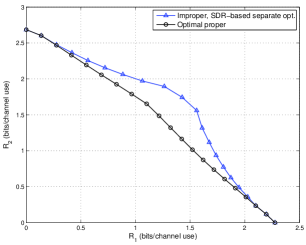
Figure 1: Achievable rate region for the two-user MISO-IC with $M=2$, SNR = 10 dB, and channel realization $\mathbf{H}^{(1)}$.

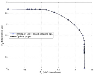
Figure 2: Achievable rate region for the two-user MISO-IC with $M=2$, SNR = 10 dB, and channel realization $\mathbf{H}^{(2)}$.

V-B Rate Region Comparison

In Fig. 1, the achievable rate region for an example two-user MISO-IC with $M=2$ is plotted for SNR=$10$ dB, with the channel realization (denoted as $\mathbf{H}^{(1)}$) given in the left column of Table II. The proposed improper Gaussian signaling with SDR-based separate covariance and pseudo-covariance optimization is compared against the optimal proper Gaussian signaling obtained by solving (P1.1). It is observed that for this channel setup, the achievable rate region has been significantly enlarged by the proposed pseudo-covariance optimization for improper Gaussian signaling.

Next, we consider a different channel realization $\mathbf{H}^{(2)}$, which differs from $\mathbf{H}^{(1)}$ only in the phases of the second elements in $\mathbf{h}_{21}$ and $\mathbf{h}_{12}$, as shown in the right column of Table II. It is observed from Fig. 2 that for this new channel setup, there is no notable rate gain by the proposed improper Gaussian signaling over the optimal proper signaling, which is in sharp contrast to the result in Fig. 1. This can be explained by comparing the residue interference levels after applying the optimal proper Gaussian signaling in the two cases. It is worth noting that for the two-user MISO-IC, the optimal proper Gaussian signaling at each transmitter is known to be a linear combination of the ZF beamforming and the maximum ratio transmission (MRT) [4]. Applying this result to the two-user MISO-IC in our context, it then follows that one user will generate less amount of interference to the other user if its direct channel and interfering channel vectors are more close to be orthogonal. Let $\theta_{1}$ denote the angle between the direct and interfering channel vectors for transmitter $1$, i.e., $\cos\theta_{1}\triangleq|\mathbf{h}_{21}\mathbf{h}_{11}^{H}|/(\|\mathbf{h}_{21}\|\|\mathbf{h}_{11}\|)$, and define $\theta_{2}$ for transmitter $2$ similarly. As shown in Table II, since $\theta_{1}$ and $\theta_{2}$ are smaller in the case of $\mathbf{H}^{(1)}$ than that in the case of $\mathbf{H}^{(2)}$, more substantial interference is resulted even after applying the optimal proper transmit beamforming. As a result, further optimization over the pseudo-covariance matrices provides more significant rate gains in the case of $\mathbf{H}^{(1)}$ than that of $\mathbf{H}^{(2)}$, which is consistent with our discussion in Remark 2.

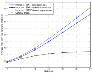
Figure 3: Average max-min rate for the two-user SISO-IC.

V-C Max-Min Rate Comparison

The rate-profile technique used in characterizing the Pareto boundary of the achievable rate region can be directly applied for maximizing the minimum (max-min) rate of all users without time sharing. Specifically, the max-min problem for the $K$-user MISO-IC is equivalent to solving (P1) by using the rate-profile $\bm{\alpha}=1/K\mathbf{1}$. In this subsection, the average max-min rate achievable over $1000$ random channel realizations by the proposed improper Gaussian signaling is compared with that by the optimal proper Gaussian signaling obtained by solving (P1.1).

Figure 4: Average max-min rate for the three-user MISO-IC with $M=2$.

We first consider the special case of the two-user SISO-IC, where two alternative improper Gaussian signaling designs proposed in [23], one with SDR-based joint covariance and pseudo-covariance optimization and the other with SOCP-based separate covariance and pseudo-covariance optimization, are compared with the proposed SDR-based separate covariance and pseudo-covariance optimization. It is observed in Fig. 3 that improper Gaussian signaling provides significant rate gains over the optimal proper Gaussian signaling. At high SNR, the max-min rate by proper Gaussian signaling saturates, since the total number of data streams transmitted, which is $2$, exceeds the total number of DoF of the two-user SISO-IC, which is known to be $1$. In contrast, a linear increase of the max-min rate with respect to the logarithm of SNR is observed by improper Gaussian signaling. It is also observed that the two separate covariance and pseudo-covariance optimization algorithms, SDR-based or SOCP-based, provide the same max-min rate performance in the case of $K=2$. This is as expected since both algorithms achieve the global optimality for the covariance and pseudo-covariance optimization subproblems in the two-user SISO-IC case. Moreover, it is observed in Fig. 3 that the SDR-based joint covariance and pseudo-covariance optimization algorithm in [23] achieves additional rate gains over the SDR/SOCP-based separate optimization. However, the extension of such a joint optimization to the general $K$-user MISO-IC with $K>2$ and/or $M>1$ remains unknown.

To show the max-min rate performance with improper Gaussian signaling when there are multiple transmit antennas, we consider a three-user MISO-IC with $M=2$. As shown in Fig. 4, a significant rate improvement is observed by the proposed improper Gaussian signaling over the optimal proper Gaussian signaling.

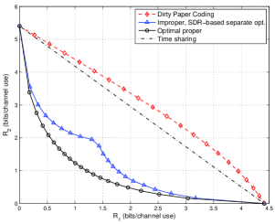
Figure 5: Achievable rate region for the two-user MISO-BC with $M=2$ and SNR = 10 dB.

V-D Rate Region of MISO-BC

At last, MISO-BC with improper Gaussian signaling or widely linear precoding as discussed in Section IV is considered. In Fig. 5, the achievable rate regions for an example two-user MISO-BC with $M=2$ are plotted for SNR = 10 dB. The channel vectors of the two users are respectively given by $\mathbf{h}_{1}=[\begin{matrix}1.1741e^{1.0030i}&0.8064e^{2.8642i}\end{matrix}]$, $\mathbf{h}_{2}=[\begin{matrix}1.8116e^{2.0647i}&0.9209e^{-2.4167i}\end{matrix}]$. The proposed improper Gaussian signaling is compared with the optimal proper Gaussian signaling with linear beamforming. As a benchmark, the capacity region achieved by the nonlinear DPC with proper Gaussian signaling is also included. It is observed that without time sharing of the achievable users’ rates by a convex-hull operation, the achievable rate region for the MISO-BC is significantly enlarged by employing improper Gaussian signaling over the optimal proper Gaussian signaling. However, such a rate gain no longer exists if time sharing is performed.

VI Conclusion

This paper has studied the transmit optimization problem for the $K$-user MISO-IC with the interference treated as noise, when improper or circularly asymmetric complex Gaussian signaling is applied. By exploiting the separable achievable rate structure with improper Gaussian signaling, a separate transmit covariance and pseudo-covariance optimization algorithm has been proposed. For the pseudo-covariance optimization, we have established the optimality of rank-1 pseudo-covariance matrices, given the optimal rank-1 transmit covariance matrices obtained by existing methods. Moreover, we have shown that each rank-1 pseudo-covariance matrix is parameterized by one unknown complex scalar and thereby the complexity for searching is greatly reduced. We then applied the SDR technique to find an efficient approximate solution for the pseudo-covariance optimization problem. The proposed improper Gaussian signaling has been extended to MISO-BC with widely linear precoding. Finally, numerical results have been provided to demonstrate the achievable rate gains over conventional proper Gaussian signaling in various multiuser multi-antenna systems that can be modeled by the MISO-IC.

Appendix A Proof of Lemma 1

The following result will be used for proving Lemma 1.

Lemma 2.

[31] If $\mathbf{X}$ is Hermitian and is partitioned as $\mathbf{X}=\left[\begin{matrix}\mathbf{A}&\mathbf{B}\\ \mathbf{B}^{H}&\mathbf{C}\end{matrix}\right]$, then $\mathbf{X}\succeq\mathbf{0}$ if and only if the following three conditions are satisfied:

$$(a)\ \mathbf{A}\succeq\mathbf{0};\ (b)\ (\mathbf{I}-\mathbf{A}\mathbf{A}^{\dagger})\mathbf{B}=\mathbf{0};\ (c)\ \mathbf{C}-\mathbf{B}^{H}\mathbf{A}^{\dagger}\mathbf{B}\succeq\mathbf{0},$$

where $(\cdot)^{\dagger}$ represents the Moore- Penrose pseudo-inverse.

We now re-express the positive semidefinite constraint in (12) using the above three conditions. First, it is clear that $(a)$ is guaranteed in (12). Next, to use the condition in $(b)$, we express the singular value decomposition (SVD) of the rank-1 covariance matrix $\mathbf{C}_{\mathbf{x}_{k}}^{\star}$ as

$$\mathbf{C}_{\mathbf{x}_{k}}^{\star}=\mathbf{t}_{k}\mathbf{t}_{k}^{H}=\left[\begin{matrix}\widetilde{\mathbf{t}}_{k}&\mathbf{U}_{k}\end{matrix}\right]\left[\begin{matrix}\|\mathbf{t}_{k}\|^{2}&\mathbf{0}\\ \mathbf{0}&\mathbf{0}\end{matrix}\right]\left[\begin{matrix}\widetilde{\mathbf{t}}_{k}^{H}\\ \mathbf{U}_{k}^{H}\end{matrix}\right],$$

where $\widetilde{\mathbf{t}}_{k}=\mathbf{t}_{k}/\|\mathbf{t}_{k}\|$, and $\mathbf{U}_{k}\in\mathbb{C}^{M\times(M-1)}$ satisfies $\mathbf{U}_{k}^{H}\mathbf{U}_{k}=\mathbf{I}_{M-1}$, and $\widetilde{\mathbf{t}}_{k}^{H}\mathbf{U}_{k}=\mathbf{0}$. Then the Moore- Penrose pseudo-inverse of $\mathbf{C}_{\mathbf{x}_{k}}^{\star}$ can be obtained as

$$(\mathbf{C}_{\mathbf{x}_{k}}^{\star})^{\dagger}=\|\mathbf{t}_{k}\|^{-2}\widetilde{\mathbf{t}}_{k}\widetilde{\mathbf{t}}_{k}^{H}.$$

Applying the condition in $(b)$ of Lemma 2 to (12) yields

$$\left(\mathbf{I}-\mathbf{C}_{\mathbf{x}_{k}}^{\star}(\mathbf{C}_{\mathbf{x}_{k}}^{\star})^{\dagger}\right)\widetilde{\mathbf{C}}_{\mathbf{x}_{k}}=\mathbf{0} \Longleftrightarrow(\mathbf{I}-\widetilde{\mathbf{t}}_{k}\widetilde{\mathbf{t}}_{k}^{H})\widetilde{\mathbf{C}}_{\mathbf{x}_{k}}=\mathbf{0}$$

$$\Longleftrightarrow\widetilde{\mathbf{C}}_{\mathbf{x}_{k}}=\widetilde{\mathbf{t}}_{k}\mathbf{v}_{k}^{H}$$ (31)

$$\Longleftrightarrow\widetilde{\mathbf{C}}_{\mathbf{x}_{k}}=\gamma_{k}\widetilde{\mathbf{t}}_{k}\mathbf{\widetilde{v}}_{k}^{H},$$ (32)

where $\mathbf{v}_{k}\in\mathbb{C}^{M\times 1}$ is an arbitrary vector with its Euclidian norm denoted by $\gamma_{k}$ and normalized direction by $\mathbf{\tilde{v}}_{k}$. To show both the “if” and “only if” conditions in (31), we first note that $\widetilde{\mathbf{C}}_{\mathbf{x}_{k}}=\widetilde{\mathbf{t}}_{k}\mathbf{v}_{k}^{H}$ is a solution of $(\mathbf{I}-\widetilde{\mathbf{t}}_{k}\widetilde{\mathbf{t}}_{k}^{H})\widetilde{\mathbf{C}}_{\mathbf{x}_{k}}=\mathbf{0}$. In addition, any solution $\widetilde{\mathbf{C}}_{\mathbf{x}_{k}}$ of the equation $(\mathbf{I}-\widetilde{\mathbf{t}}_{k}\widetilde{\mathbf{t}}_{k}^{H})\widetilde{\mathbf{C}}_{\mathbf{x}_{k}}=\mathbf{0}$ must satisfy $\widetilde{\mathbf{C}}_{\mathbf{x}_{k}}=\widetilde{\mathbf{t}}_{k}(\widetilde{\mathbf{C}}_{\mathbf{x}_{k}}^{H}\widetilde{\mathbf{t}}_{k})^{H}$, which confirms the existence of a vector $\mathbf{v}_{k}=\widetilde{\mathbf{C}}_{\mathbf{x}_{k}}^{H}\widetilde{\mathbf{t}}_{k}$ such that $\widetilde{\mathbf{C}}_{\mathbf{x}_{k}}=\widetilde{\mathbf{t}}_{k}\mathbf{v}_{k}^{H}$.

Since $\widetilde{\mathbf{C}}_{\mathbf{x}_{k}}$ is a pseudo-covariance matrix, which must be symmetric, we have

$$\widetilde{\mathbf{C}}_{\mathbf{x}_{k}}=\gamma_{k}\widetilde{\mathbf{t}}_{k}\mathbf{\widetilde{v}}_{k}^{H}=\gamma_{k}\mathbf{\widetilde{v}}_{k}^{*}\widetilde{\mathbf{t}}_{k}^{T}=\widetilde{\mathbf{C}}_{\mathbf{x}_{k}}^{T}.$$

By expressing $\widetilde{\mathbf{C}}_{\mathbf{x}_{k}}\widetilde{\mathbf{C}}_{\mathbf{x}_{k}}^{H}$ using two alternative forms, we have

$$\widetilde{\mathbf{C}}_{\mathbf{x}_{k}}\widetilde{\mathbf{C}}_{\mathbf{x}_{k}}^{H}=\gamma_{k}^{2}\widetilde{\mathbf{t}}_{k}\widetilde{\mathbf{t}}_{k}^{H}=\gamma_{k}^{2}\mathbf{\widetilde{v}}_{k}^{*}(\mathbf{\widetilde{v}}_{k}^{*})^{H}$$

$$\Longleftrightarrow\widetilde{\mathbf{t}}_{k}=e^{i\theta_{k}}\mathbf{\widetilde{v}}_{k}^{*},\text{ or }\mathbf{\widetilde{v}}_{k}=e^{i\theta_{k}}\widetilde{\mathbf{t}}_{k}^{*},$$ (33)

where $\theta_{k}\in[0,2\pi)$. By substituting $\mathbf{v}_{k}$ into (32), we have

$$\widetilde{\mathbf{C}}_{\mathbf{x}_{k}}=\gamma_{k}e^{-i\theta_{k}}\widetilde{\mathbf{t}}_{k}\widetilde{\mathbf{t}}_{k}^{T}=Z_{k}\widetilde{\mathbf{t}}_{k}\widetilde{\mathbf{t}}_{k}^{T},$$ (34)

where we have defined the complex variable $Z_{k}=\gamma_{k}e^{-i\theta_{k}}$. Furthermore, the condition in $(c)$ of Lemma 2 implies that for the constraint in (12) to be satisfied, we need to have

$$(\mathbf{C}_{\mathbf{x}_{k}}^{\star})^{*}-\widetilde{\mathbf{C}}_{\mathbf{x}_{k}}^{*}(\mathbf{C}_{\mathbf{x}_{k}}^{\star})^{\dagger}\widetilde{\mathbf{C}}_{\mathbf{x}_{k}}\succeq\mathbf{0}$$

$$\Longleftrightarrow\left(\|\mathbf{t}_{k}\|^{2}-|Z_{k}|^{2}\|\mathbf{t}_{k}\|^{-2}\right)\widetilde{\mathbf{t}}_{k}^{*}\widetilde{\mathbf{t}}_{k}^{T}\succeq\mathbf{0}$$

$$\Longleftrightarrow|Z_{k}|\leq\|\mathbf{t}_{k}\|^{2}.$$ (35)

This thus completes the proof of Lemma 1.

Appendix B Proof of Theorem 1

Since the inequalities in (23) and (24) of Theorem 1 can be proved similarly, for brevity, we only show the proof of (23) in this appendix. First, if $\mathbf{W}_{k}=\mathbf{w}_{k}\mathbf{w}_{k}^{H}=\mathbf{0}$, i.e., $\mathbf{w}_{k}$ is a zero-vector, then (23) is satisfied since

$$C_{s_{k}}^{2}=(\sum_{j\neq k}|\mathbf{h}_{kj}\mathbf{t}_{j}|^{2}+\sigma^{2})^{2}\geq\sigma^{4}$$ (36)

is true. Therefore, in the following, we assume without loss of generality that at least one of the elements in $\mathbf{w}_{k}$ is non-zero. Then we consider the following optimization problem.

$$\text{(P-A1):}\ \underset{\mathbf{Z}\succeq\mathbf{0}}{\mathrm{max.}}\ \mathrm{Tr}(\mathbf{W}_{k}\mathbf{Z})=\mathrm{Tr}(\mathbf{w}_{k}\mathbf{w}_{k}^{H}\mathbf{Z})$$

s.t. $$\mathrm{Tr}(\mathbf{E}_{k}\mathbf{Z})\leq\big{\|}\mathbf{t}_{k}\big{\|}^{4},\ \forall k.$$ (37)

In order to show (23) in Theorem 1, it is sufficient to prove that the optimal objective value of (P-A1) is no greater than $1-C_{s_{k}}^{-2}\sigma^{4}$. With (36), this is clearly true if the optimal solution $\mathbf{Z}^{\star}$ to (P-A1) is a zero matrix. Therefore, in the following, we assume $\mathbf{Z}^{\star}\neq\mathbf{0}$. The following result, whose proof can be found in Lemma I of [34] or in Lemma 1.6 of [26], will be used.

Lemma 3.

There exists a rank-1 optimal solution to (P-A1).

With Lemma 3, (P-A1) can be re-expressed as

$$\text{(P-A2):}\ \underset{\mathbf{z}}{\mathrm{max.}} \ \mathbf{z}^{H}\mathbf{W}_{k}\mathbf{z}$$

s.t. $$\ |\mathbf{e}_{k}^{H}\mathbf{z}\big{|}^{2}\leq\big{\|}\mathbf{t}_{k}\big{\|}^{4},\ \forall k.$$ (38)

Using (14) and (16), we have

$$\mathbf{z}^{H}\mathbf{W}_{k}\mathbf{z} =C_{s_{k}}^{-2}\Big{|}\sum_{j\neq k}(\mathbf{h}_{kj}\widetilde{\mathbf{t}}_{j})^{2}Z_{j}\Big{|}^{2}$$

$$\leq C_{s_{k}}^{-2}\Big{(}\sum_{j\neq k}|\mathbf{h}_{kj}\widetilde{\mathbf{t}}_{j}|^{2}|Z_{j}|\Big{)}^{2}$$ (39)

$$\leq C_{s_{k}}^{-2}\Big{(}\sum_{j\neq k}|\mathbf{h}_{kj}\widetilde{\mathbf{t}}_{j}|^{2}\|\mathbf{t}_{j}\|^{2}\Big{)}^{2}$$ (40)

$$\leq C_{s_{k}}^{-2}\Big{[}\Big{(}\sum_{j\neq k}|\mathbf{h}_{kj}\mathbf{t}_{j}|^{2}+\sigma^{2}\Big{)}^{2}-\sigma^{4}\Big{]}$$ (41)

$$=1-C_{s_{k}}^{-2}\sigma^{4}.$$ (42)

where (39) is due to the triangle inequality; (40) is due to the constraint in (38), which is equivalent to $|Z_{k}|\leq\|\mathbf{t}_{k}\|^{2},\forall k$; and (42) is true since $C_{s_{k}}=\sum_{j\neq k}|\mathbf{h}_{kj}\mathbf{t}_{j}|^{2}+\sigma^{2}$. The above result shows that the optimal objective value of (P-A2), and hence that of (P-A1), is no larger than $1-C_{s_{k}}^{-2}\sigma^{4}$, as desired.

This thus completes the proof of Theorem 1.

References

- [1] R. Etkin, D. Tse, and H. Wang, “Gaussian interference channel capacity to within one bit,” IEEE Trans. Inf. Theory, vol. 54, no. 1, pp. 5534–5562, Dec. 2008.
- [2] M. Charafeddine, A. Sezgin, and A. Paulraj, “Rates region frontiers for -user interference channel with interference as noise,” in Proc. Allerton Conference, Sep. 2007.
- [3] L. Liu, R. Zhang, and K.-C. Chua, “Achieving global optimality for weighted sum-rate maximization in the -user Gaussian interference channel with multiple antennas,” IEEE Trans. Wireless Commun., vol. 11, no. 5, pp. 1933–1945, May 2012.
- [4] E. Jorswieck, E. Larsson, and D. Danev, “Complete characterization of the Pareto boundary for the MISO interference channel,” IEEE Trans. Signal Process., vol. 56, no. 10, pp. 5292–5296, Oct. 2008.
- [5] R. Zhang and S. Cui, “Cooperative interference management with MISO beamforming,” IEEE Trans. Signal Process., vol. 58, no. 10, pp. 5450–5458, Oct. 2010.
- [6] X. Shang, B. Chen, and H. V. Poor, “Multiuser MISO interference channles with single-user detection: optimality of beamforming and the achievable rate region,” IEEE Trans. Inf. Theory, vol. 57, no. 7, pp. 4255 – 4273, Jul. 2011.
- [7] R. Mochaourab and E. A. Jorswieck, “Optimal beamforming in interference networks with perfect local channel information,” IEEE Trans. Signal Process., vol. 59, no. 3, pp. 1128–1141, Mar. 2011.
- [8] A. Gjendemsj, D. Gesbert, G. E. ien, and S. G. Kiani, “Binary power control for sum rate maximization over multiple interfering links,” IEEE Trans. Wireless Commun., vol. 7, no. 8, pp. 3164–3173, Aug. 2008.
- [9] Y.-F. Liu, Y.-H. Dai, and Z.-Q. Luo, “Coordinated beamforming for MISO interference channel: complexity analysis and efficient algorithms,” IEEE Trans. Signal Process., vol. 59, no. 3, pp. 1142–1156, Mar. 2011.
- [10] S. Ye and R. S. Blum, “Optimized signaling for MIMO interference systems with feedback,” IEEE Trans. Signal Process., vol. 51, no. 11, pp. 2839–2848, Nov. 2003.
- [11] J. Huang, R. A. Berry, and M. L. Honig, “Distributed interference compensation for wireless networks,” IEEE J. Sel. Areas Commun., vol. 24, no. 5, pp. 1074–1084, May 2006.
- [12] G. Scutari, P. Palomar, and S. Barbarossa, “The MIMO iterative waterfilling algorithm,” IEEE Trans. Signal Process., vol. 57, no. 5, pp. 1917–1935, May 2009.
- [13] Q. Shi, M. Razaviyayn, Z.-Q. Luo, and C. He, “An iteratively weighted MMSE approach to distributed sum-utility maximization for a MIMO interfering broadcast channel,” IEEE Trans. Signal Process., vol. 59, no. 9, pp. 4331–4340, Sep. 2011.
- [14] L. P. Qian, Y. J. Zhang, and J. Huang, “MAPEL: achieving global optimality for a non-convex wireless power control problem,” IEEE Trans. Wireless Commun., vol. 8, no. 3, pp. 1553–1563, Mar. 2009.
- [15] E. A. Jorswieck and E. G. Larsson, “Monotonic optimization framework for the two-user miso interference channel,” IEEE Trans. Commun., vol. 58, no. 7, pp. 2159–2168, Jul. 2010.
- [16] W. Utschick and J. Brehmer, “Monotonic optimization framework for coordinated beamforming in multicell networks,” IEEE Trans. Signal Process., vol. 60, no. 4, pp. 1899–1909, Apr. 2012.
- [17] E. Björnson, G. Zheng, M. Bengtsson, and B. Ottersten, “Robust monotonic optimization framework for multicell MISO systems,” IEEE Trans. Signal Process., vol. 60, no. 5, pp. 2508–2523, May 2012.
- [18] S. A. Jafar, Interference Alignment: A New Look at Signal Dimensions in a Communication Network. Foundations and Trends in Communications and Information Theory, 2010, vol. 7, no. 1.
- [19] B. Picinbono and P. Chevalier, “Widely linear estimation with complex data,” IEEE Trans. Signal Process., vol. 43, no. 8, pp. 2030–2033, Aug. 1995.
- [20] V. R. Cadambe, S. A. Jafar, and C. Wang, “Interference alignment with asymmetric complex signaling - settling the Host-Madsen-Nosratinia conjecture,” IEEE Trans. Inf. Theory, pp. 4552 – 4565, Sep. 2010.
- [21] Z. K. M. Ho and E. Jorswieck, “Improper Gaussian signaling on the two-user SISO interference channel,” IEEE Trans. Wireless Commun., vol. 11, no. 9, pp. 3194 – 3203, Sep. 2012.
- [22] H. Park, S. H. Park, J. S. Kim, and I. Lee, “SINR balancing techniques in coordinated multi-cell downlink systems,” IEEE Trans. Wireless Commun., vol. 12, no. 2, pp. 626–635, Feb. 2013.
- [23] Y. Zeng, C. M. Yetis, E. Gunawan, Y.-L. Guan, and R. Zhang, “Transmit optimization with improper Gaussian signaling for interference channels,” IEEE Trans. Signal Process., vol. 61, no. 11, pp. 2899–2913, Jun. 2013.
- [24] Z.-Q. Luo, W. K. Ma, A. M. So, Y. Ye, and S. Zhang, “Semidefinite relaxation of quadratic optimization problems,” IEEE Signal Processing Mag, vol. 27, no. 3, pp. 20–34, May 2010.
- [25] H. Weingarten, Y. Steinberg, and S. Shamai (Shitz), “The capacity region of the Gaussian multiple-input multiple-output broadcast channel,” IEEE Trans. Inf. Theory, vol. 52, no. 9, pp. 3936–3964, Sep. 2006.
- [26] E. Björnson and E. Jorswieck, “Optimal resource allocation in coordinated multi-cell systems,” Foundations and Trends in Communications and Information Theory, vol. 9, no. 2-3, pp. 113–381, 2013.
- [27] T. Adali, P. J. Schreier, and L. L. Scharf, “Complex-valued signal processing: The proper way to deal with impropriety,” IEEE Trans. Signal Process., vol. 59, no. 11, pp. 5101–5125, Nov. 2011.
- [28] P. J. Schreier and L. L. Scharf, Statistical Signal Processing of Complex-Valued Data: The Theory of Improper and Noncircular Signals. Cambridge Univ. Press, 2010.
- [29] E. Telatar, “Capacity of multi-antenna Gaussian channels,” European Trans. Tel., vol. 10, no. 6, pp. 585–596, Nov. 1999.
- [30] A. Wiesel, Y. C. Eldar, and S. Shamai (Shitz), “Linear precoding via conic optimization for fixed MIMO receivers,” IEEE Trans. Signal Process., vol. 54, no. 1, pp. 161–176, Jan. 2006.
- [31] S. Boyd and L. Vandenberghe, Convex Optimization. Cambridge, U.K.: Cambridge Univ. Press, 2004.
- [32] Y. Huang and D. P. Palomar, “Rank-constrained separable semidefinite programming with applications to optimal beamforming,” IEEE Trans. Signal Process., vol. 58, no. 2, pp. 664–678, Feb. 2010.
- [33] C. Hellings and W. Utschick, “Performance gains due to improper signals in MIMO broadcast channels with widely linear transceivers,” in Int. Conf. on Acoustics, Speech, and Signal Process., Vancouver, Canada, May 26-31, 2013.
- [34] A. Wiesel, Y. C. Eldar, and S. Shamai, “Zero-forcing precoding and generalized inverses,” IEEE Trans. Signal Process., vol. 55, no. 9, pp. 4409–4418, Sep. 2008.