Protecting Dissipative Quantum State Preparation via Dynamical Decoupling

Abstract

We show that dissipative quantum state preparation processes can be protected against qubit dephasing by interlacing the state preparation control with dynamical decoupling (DD) control consisting of a sequence of short $\pi$-pulses. The inhomogeneous broadening can be suppressed to second order of the pulse interval, and the protection efficiency is nearly independent of the pulse sequence but determined by the average interval between pulses. The DD protection is numerically tested and found to be efficient against inhomogeneous dephasing on two exemplary dissipative state preparation schemes that use collective pumping to realize many-body singlets and linear cluster states respectively. Numerical simulation also shows that the state preparation can be efficiently protected by $\pi$-pulses with completely random arrival time. Our results make possible the application of these state preparation schemes in inhomogeneously broadened systems. DD protection of state preparation against dynamical noises is also discussed using the example of Gaussian noise with a semiclasscial description.

I Introduction

Dissipative quantum state preparation has recently emerged as a conceptually new approach for realizing resources of multipartite quantum entanglement. In the control of an open quantum system, dissipative channels are usually the sources of errors and play deleterious roles. However, by properly tailoring the dissipative channels in an open quantum system, the irreversible dynamics can have steady states containing the important resource of quantum entanglement. Earlier studies in small scale systems have shown that two-qubit entanglement can be generated in the steady states of various dissipative dynamics driven either by external incoherent pumping or by the tailored coupling with the environment 1 ; 2 ; 3 ; 4 . Recent studies have lead to the discovery of various dissipative state preparation approaches for realizing multipartite entanglement in large scale systems 5 ; 6 ; 7 ; 8 ; 9 ; 10 ; 11 ; 12 ; 13 . In particular, it has been shown that by using only a few incoherent pumping channels that couple collectively to the qubits, various types of multipartite entanglement can be prepared, including the linear cluster states 10 , many-body singlet states 11 , and symmetric and asymmetric Dicke states 12 ; 13 . These multipartite entangled states can be the crucial resource for measurement based quantum information processing 1b ; 2b ; 3b ; 4b . With the desired quantum states unconditionally realizable as steady states of the irreversible dynamics, the dissipative state preparation schemes have the advantage of robustness and do not need accurate temporal controls as compared to conventional state preparation by coherent evolutions.

Most dissipative state preparation schemes are proposed for qubit systems with homogeneous resonances 1 ; 2 ; 3 ; 4 ; 10 ; 11 ; 12 ; 13 . In reality, the qubit resonance can have inevitable inhomogeneous broadening which leads to inhomogeneous dephasing. Moreover, fluctuation of the environment can also induce dynamical noise that leads to dephasing as well. These unwanted noise channels will compete with the tailored dissipative channels for preparing quantum entanglement in the irreversible dynamics. The fidelity of the steady state with the target quantum state will decrease with the increase of the noise strength and the number of qubits. These inevitable noises will render the state preparation scheme impractical in large scale systems in the presence of inhomogeneous broadening and dynamical noise. Whether or not we can suppress the noises while preserving the desired dissipative channels in the irreversible dynamics becomes the key.

Dynamical decoupling (DD) has been an extensively explored approach in high-precision magnetic resonance spectroscopy 14 ; 15 ; 16 ; 17 , and for suppressing the effect of qubit dephasing in quantum information processing 18 ; 19 ; 20 ; 21 . The basic idea is to introduce a sequence of pulses on the qubit in order to average out the inhomogeneous broadening and the unwanted coupling with the environment, hence eliminating the noise effects on the qubit. Past studies on dynamical decoupling have focused on how to freeze the evolution of a qubit prepared on an arbitrary quantum state such that the quantum memory time can be enhanced. One efficient DD approach for protecting quantum memory uses sequences of instantaneous $\pi$-pulses with properly chosen arrival time. Inhomogeneous dephasing can be removed transiently at a certain time known as the spin echo time, while dynamical noises can also be suppressed to high orders at the spin echo times depending on the pulse sequences. The protection of coherent evolutions by DD control pulses has also been studied 36 ; gate1 ; gate ; gate2 ; gate3 .

In this paper, we show that dissipative quantum state preparation processes can be protected against qubit dephasing by interlacing the dissipative control with DD control consisting of sequences of $\pi$-pulses. The DD control is introduced here to suppress the qubit dephasing while preserving a nontrivial irreversible evolution for generating entanglement in the steady state. For suppression of inhomogeneous dephasing, we compare DD controls consisting of repetitions of a basic unit which takes various designs including the Carr-Purcell-Meiboom-Gill (CPMG) 22 ; 23 , concatenated (CDD) 24 ; 25 ; 26 ; 27 ; 28 ; 29 , and Uhrig sequences (UDD) 30 ; 31 ; 32 ; 33 . We found the leading noise term in the Magnus expansion is of second order of the pulse interval and the residue effect of inhomogeneous dephasing is largely determined by the average pulse interval only, nearly independent of the types of the DD pulse sequences. High fidelity state preparation is therefore possible even in the presence of substantial inhomogeneous broadening when the DD pulse sequence with sufficiently small pulse interval is applied. DD protection from dynamical noise is discussed for the example of Gaussian noise of a semiclassical description, where the leading noise effect is also found to be of second order of the pulse interval. The order of noise suppression is qualitatively different from that in the DD protection of quantum memory because of the presence of the state-preparation channel, and its interference with the noise channels determines the residue noise effect.

For the scheme of preparing the many-body singlet 11 ; 12 , we perform systematic numerical simulations of the DD protection against inhomogeneous dephasing using CPMG, concatenated, and Uhrig pulse sequences. We find that the Magnus expansion converges well and the residue inhomogeneous broadening effect is well accounted by the leading noise term in the Magnus series. Numerical simulation confirms that the protection efficiency is nearly independent of the pulse sequence and depends only on the average pulse interval. Moreover, the application of $\pi$-pulses with completely random arrival time 34 ; 35 is found to be efficient in suppressing the effect of inhomogeneous broadening. Thus, the DD protection is robust against errors in the pulse arrival time. We also explain how to implement the DD protection on the scheme of preparing linear cluster states 10 , where our numerical simulation confirms that high fidelity state preparation can be realized in the presence of substantial inhomogeneous broadening through the DD control. These dissipative preparation schemes for preparing the two important classes of multipartite entanglement are therefore applicable to inhomogeneously broadened qubit systems.

The paper is organized as follows. In section II, we discuss the basic idea of protecting dissipative quantum state preparation against noise channels by interlacing the state-preparation control with the DD control pulses. The evolution of the system is expanded in terms of the Magnus series. In section III, we discuss the DD protection of the state preparation against inhomogeneous dephasing, and derive coefficients of Magnus series for investigating the order of noise suppression. In section IV, we discuss the DD protection on the preparation of many-body singlet states against inhomogeneous dephasing and show numerical simulation results. In section V, we numerically study the DD protection of the linear cluster states in the presence of inhomogeneous dephasing. In section VI, DD protection against dynamical noise is discussed for the example of Gaussian noise of a semiclassical description. Finally, the conclusions are summarized in section VII.

II Magnus Expansion

In the dissipative quantum state preparation, the evolution of the open quantum system is described by the master equation as $\dot{\rho}=\mathcal{L}_{\mathrm{P}}\left[\rho\right]$, where $\rho$ is the density matrix of the system and $\mathcal{L}_{\mathrm{P}}\left[\rho\right]$ is the super-operator describing the dissipative dynamics tailored for generating entanglement. In a typical dissipative quantum state preparation process 1 ; 2 ; 3 ; 4 ; 5 ; 6 ; 7 ; 8 ; 9 ; 10 ; 11 ; 12 ; 13 , the dissipative channels $\mathcal{L}_{\mathrm{P}}$ are time independent and are engineered such that the desired entangled states are obtained as the steady states of the irreversible dynamics.

In reality, there exist other noise channels which also affect the system dynamics as denoted by the super-operator $\mathcal{L}_{\mathrm{N}}\left[\rho\right]$, which can have various origins such as inhomogeneous broadening of the level spacing, and dynamical fluctuation from the coupling with an environment. The unwanted evolution $\mathcal{L}_{\mathrm{N}}\left[\rho\right]$ will compete with the tailored dissipative dynamics $\mathcal{L}_{\mathrm{P}}\left[\rho\right]$. As a result, the steady state of the dynamics $\dot{\rho}=\mathcal{L}_{\mathrm{P}}\left[\rho\right]+\mathcal{L}_{\mathrm{N}}\left[\rho\right]$ deviates from the target entangled state. The state preparation fidelity will drop with the increase of the noise strength and the number of qubits. To achieve high fidelity state preparation in large scale systems, the undesired noise channels $\mathcal{L}_{\mathrm{N}}$ need to be suppressed while preserving the desired dissipative dynamics $\mathcal{L}_{\mathrm{P}}\left[\rho\right]$ at the same time.

We consider interlacing the state-preparation control with the DD control consisting of a sequence of short pulses which realize the unitary rotations $U_{i}$ at time $\tau_{i}$ on all qubits. If the duration of the pulse is much smaller than the pulse interval, the rotation can be considered as instantaneous. It is convenient to analyze the evolution of the system in the toggling frame that follows these rotations of the qubits. In the toggling frame, the super-operators for the noise channels and the desired dissipative channels become: $\mathcal{L}_{\mathrm{N}}^{\mathrm{T}}\left[t;\rho\right]=U(t)\mathcal{L}_{\mathrm{N}}\left[\rho\right]U(t)^{\dagger}$ and $\mathcal{L}_{\mathrm{P}}^{\mathrm{T}}\left[t;\rho\right]=U(t)\mathcal{L}_{\mathrm{P}}\left[\rho\right]U(t)^{\dagger},$ where $U(t)\equiv\prod_{j=1}^{i}U_{j}$ for $\tau_{i}<t<\tau_{i+1}$. Below we focus on DD control using sequences of short $\pi$ pulses (see Fig. 1). In such case, $U_{i}=\sigma_{x}$, and we have $U(t)=\sigma_{x}$ in the odd intervals (i.e. $\tau_{i}<t<\tau_{i+1}$ with odd $i$), and $U(t)=I$ in the even intervals (i.e. $\tau_{i}<t<\tau_{i+1}$ with even $i$).

If the noise super-operators in the toggling frame have overall sign changes for adjacent intervals as $\mathcal{L}_{\mathrm{N}}^{\mathrm{T}}\left[t;\rho\right]=f(t)\mathcal{L}_{\mathrm{N}}\left[\rho\right]$, where $f(t)=(-1)^{i}$ for $\tau_{i}<t<\tau_{i+1}$, the effect of the noise can then be averaged out over time. This is the case for pure dephasing noise. However, in the protection of dissipative quantum state preparation, the desired dissipative channels for generating entanglement shall also be preserved. This imposes an additional requirement 36 ; gate . The simplest scenario is to require the dissipative channel to always take the desired form $\mathcal{L}_{\mathrm{P},0}$ in the toggling frame, i.e. $\mathcal{L}_{\mathrm{P}}^{\mathrm{T}}\left[t;\rho\right]=\mathcal{L}_{\mathrm{P},0}\left[\rho\right]$. Thus, in the laboratory frame, the super-operator for the dissipative channel shall alternate between the two forms $\mathcal{L}_{\mathrm{P},0}\left[\rho\right]$ and $\mathcal{L}^{\prime}_{\mathrm{P},0}\left[\rho\right]\equiv\sigma_{x}\mathcal{L}_{\mathrm{P},0}\left[\rho\right]\sigma_{x}$ in the even and odd intervals respectively (see Fig. 1). In general, $\mathcal{L}_{\mathrm{P},0}$ and $\mathcal{L}_{\mathrm{P},0}^{\prime}$ are different operators. Thus, for a dissipative state preparation protocol to be protectable by DD controls consisting of $\pi$ pulses, the dissipative dynamics shall switch between the two forms each time a $\pi$ pulse is applied if $\left[\sigma_{x},\mathcal{L}_{\mathrm{P}}\left[\rho\right]\right]\neq 0$. This can indeed be implemented in most dissipative preparation protocols as the dissipative channels $\mathcal{L}_{\mathrm{P}}\left[\rho\right]$ are engineered ones.

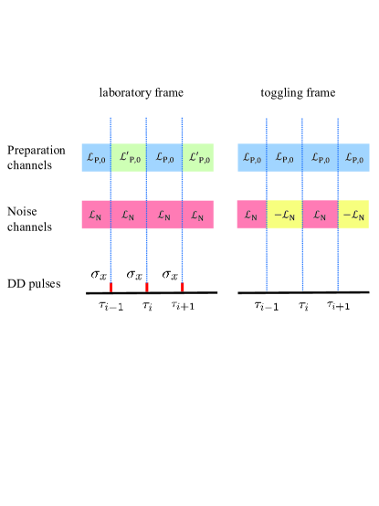
Figure 1: (Color online) Schematics of interlacing DD controls with the dissipative quantum state preparations. In the toggling frame, the noise has a sign change between odd and even time intervals and the noise effects average out over time. The effects of the dissipative preparation channel in the odd and even time intervals constructively add. In the laboratory frame, the dissipative preparation channel shall then take two different forms for the odd and even time intervals in general.

In the toggling frame, the super-operator for the dissipative preparation channel is time-independent, hence the effect adds constructively over time. The super-operator for the noise channels has alternating signs for even and odd time intervals, hence the effect destructively cancels. The master equation in the toggling frame is:

$$\dot{\rho} = \mathcal{L}_{\mathrm{P},0}[\rho]+f(t)\mathcal{L}_{\mathrm{N}}\left[\rho\right],$$ (1)

which has the formal solution:

$$\rho\left(t\right) = \mathcal{T}\exp\left[\int_{0}^{t}\left(\mathcal{L}_{\mathrm{P},0}+f(t^{\prime})\mathcal{L}_{\mathrm{N}}\right)dt^{\prime}\right]\rho\left(0\right)$$ (2)

with time ordering $\mathcal{T}$ and initial density matrix $\rho\left(0\right)$. Eq. (2) can be rewritten in terms of the Magnus expansion:

$$\rho\left(t\right) = \exp\left[\Omega\left(t\right)\right]\rho\left(0\right).$$ (3)

Here, the formal evolution operator is expanded in terms of the Magnus series as $\Omega\left(t\right)=\sum_{k=1}^{\infty}\Omega_{k}\left(t\right)$, and the first three terms of this series are:

$$\Omega_{1}\left(t\right) =\int_{0}^{t}\mathcal{L}\left[t_{1}\right]dt_{1},$$ (4a)

$$\Omega_{2}\left(t\right) =\frac{1}{2}\int_{0}^{t}\int_{0}^{t_{1}}\left[\mathcal{L}\left[t_{1}\right],\mathcal{L}\left[t_{2}\right]\right]dt_{1}dt_{2},$$ (4b)

$$\Omega_{3}\left(t\right) =\frac{1}{6}\int_{0}^{t}\int_{0}^{t_{1}}\int_{0}^{t_{2}}\left\{\left[\mathcal{L}\left[t_{1}\right],\left[\mathcal{L}\left[t_{2}\right],\mathcal{L}\left[t_{3}\right]\right]\right]+\right.$$

$$\left.\left[\mathcal{L}\left[t_{3}\right],\left[\mathcal{L}\left[t_{2}\right],\mathcal{L}\left[t_{1}\right]\right]\right]\right\}dt_{1}dt_{2}dt_{3},$$ (4c)

where $\mathcal{L}\left[t\right]=\mathcal{L}_{\mathrm{P},0}+f(t)\mathcal{L}_{\mathrm{N}}$, and $\left[\mathcal{L}\left[t_{1}\right],\mathcal{L}\left[t_{2}\right]\right]\rho\equiv\mathcal{L}\left[t_{1};\mathcal{L}\left[t_{2};\rho\right]\right]-\mathcal{L}\left[t_{2};\mathcal{L}\left[t_{1};\rho\right]\right]$ is the Poisson bracket for the super-operator $\mathcal{L}\left[t\right].$ The Magnus expansion is convergent if $\int_{0}^{t}\left\|\mathcal{L}\left[t^{\prime}\right]\right\|dt^{\prime}<\pi$, where $\left\|\mathcal{L}\right\|$ is a two-form of super-operator $\mathcal{L}$ 37 . It is convenient to investigate the suppression of noise channels with the Magnus expansion. The residue effects of noises are characterized by the leading term in the Magnus series that contains the noise operators, as we will discuss explicitly in the next section for inhomogeneous dephasing noise.

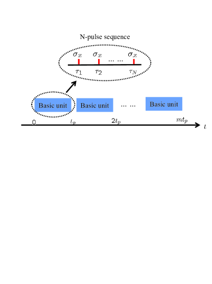
Figure 2: (Color online) Schematics of DD control, formed by repetitions of a basic unit with duration $t_{p}$. The basic unit consists of a $N$-pulse sequence which can take various designs, including the CPMG, concatenated and Uhrig sequences.

III Protection of dissipative state preparation from inhomogeneous dephasing

In this section, we investigate the protection of dissipative state preparation from inhomogeneous dephasing by the DD controls. The super-operator for this noise channel is

$$\mathcal{L}_{\mathrm{N}}\left[\rho\right] = -i\left[\sum_{i}\omega_{i}\sigma_{i}^{z},\rho\right],$$ (5)

where the inhomogeneous dephasing is the consequence of inhomogeneous broadening in the qubit resonance $\omega_{i}$. The first three terms of the Magnus expansion then become:

$$\Omega_{1}\left(t\right) = t\left[\mathcal{L}_{\mathrm{P},0}+c_{1}\left(t\right)\mathcal{L}_{\mathrm{N}}\right],$$ (6a)

$$\Omega_{2}\left(t\right) = t^{2}c_{2}\left(t\right)\left[\mathcal{L}_{\mathrm{P},0},\mathcal{L}_{\mathrm{N}}\right],$$ (6b)

$$\Omega_{3}\left(t\right) = t^{3}c_{3,a}\left(t\right)\left[\mathcal{L}_{\mathrm{P},0},\left[\mathcal{L}_{\mathrm{P},0},\mathcal{L}_{\mathrm{N}}\right]\right]$$ (6c)

$$+t^{3}c_{3,b}\left(t\right)\left[\mathcal{L}_{\mathrm{N}},\left[\mathcal{L}_{\mathrm{P},0},\mathcal{L}_{\mathrm{N}}\right]\right],$$

where $\left[\mathcal{L}_{\mathrm{P},0},\mathcal{L}_{\mathrm{N}}\right]\rho=\mathcal{L}_{\mathrm{P},0}\left[\mathcal{L}_{\mathrm{N}}\left[\rho\right]\right]-\mathcal{\mathcal{L}}_{\mathrm{N}}\left[\mathcal{L}_{\mathrm{P},0}\left[\rho\right]\right]$ stands for the Possion bracket for the super-operators. Because of the interference between the super-operators $\mathcal{L}_{\mathrm{P},0}$ and $\mathcal{L}_{\mathrm{N}}$, these Poisson brackets are typically nonzero.

Table 1: Coefficients of leading Magnus terms in Eq. (9). The coefficients are evaluated for one basic unit of evolution with duration $t_{p}$ where the DD control is a $N$-pulse sequence taking various designs (see text).

	no pulse	CPMG	CDD3	CDD4	UDD3	UDD4	UDD5
$N$	0	2	5	10	3	4	5
$\alpha_{1}$	1	0	0	0	0	0	0
$\alpha_{2}$	0	0	0	0	0	0	0
$\alpha_{3,a}$	0	$3.12\times 10^{-2}$	0	0	0	0	0
$\alpha_{3,b}$	0	$-1.04\times 10^{-2}$	$-2.60\times 10^{-3}$	$-6.51\times 10^{-4}$	$-5.05\times 10^{-3}$	$-3.04\times 10^{-3}$	$-2.04\times 10^{-3}$
$\alpha_{3,b}\times N^{2}$	0	$-4.16\times 10^{-2}$	$-6.51\times 10^{-2}$	$-6.51\times 10^{-2}$	$-4.55\times 10^{-2}$	$-4.86\times 10^{-2}$	$-5.11\times 10^{-2}$

The coefficients in Eq. (6) are given by:

$$c_{1}\left(t\right) = \frac{1}{t}\int_{0}^{t}f\left(t_{1}\right)dt_{1},$$ (7a)

$$c_{2}\left(t\right) = \frac{1}{2t^{2}}\int_{0}^{t}t_{1}g\left(t_{1}\right)dt_{1},$$ (7b)

$$c_{3,a}\left(t\right) = \frac{1}{12t^{3}}\int_{0}^{t}t_{1}^{2}h\left(t_{1}\right)dt_{1},$$ (7c)

$$c_{3,b}\left(t\right) = \frac{1}{12t^{3}}\int_{0}^{t}t_{1}^{2}\left[6c_{2}\left(t_{1}\right)f\left(t_{1}\right)-c_{1}\left(t_{1}\right)g\left(t_{1}\right)\right],$$

Here $g\left(t_{1}\right)\equiv c_{1}\left(t_{1}\right)-f\left(t_{1}\right)$ and $h\left(t_{1}\right)\equiv 6c_{2}\left(t_{1}\right)-g\left(t_{1}\right)$. Since $f(t_{1})=(-1)^{i}$ for $\tau_{i}<t_{1}<\tau_{i+1}$, if the total duration of the odd intervals equals that of the even intervals, $c_{1}$ will vanish and the leading term of the Magnus expansion $\Omega_{1}$ only contains the ideal dissipative preparation channel we wish to preserve. The residue effect of the inhomogeneous broadening is given by the higher order Magnus terms, which results from the interference of the noise channel with the preparation channel.

In the dissipative state preparation, the desired quantum state is obtained as the steady state of the dynamics, and the timescale to reach the steady state is determined by the dissipative channel $\mathcal{L}_{P,0}$. We consider a practical scenario of interlacing the DD control with the dissipative preparation (see Fig. 2). The DD control has a periodic structure which consists of repetitions of a basic unit with the duration $t_{p}$. The basic unit is an $N$-pulse sequence that can take various designs, including the CPMG 22 ; 23 , concatenated 24 ; 25 ; 26 ; 27 ; 28 ; 29 , and Uhrig 30 ; 31 ; 32 ; 33 sequences. The basic unit of the DD control can be repeated as many times as necessary along with the dissipative evolution until a steady state is reached. The average interval between the $\pi$-pulses can be defined $\bar{\tau}\equiv t_{p}/N$.

For a periodic control with period $t_{p}$, it has been proved that $\Omega_{k}\left(lt_{p}\right)=l\Omega_{k}\left(t_{p}\right)$, where $l=1,2,\ldots.$ 37 . Therefore the coefficients $c_{n}$ possess the scaling law

$$c_{n}\left(lt_{p}\right) = l^{1-n}c_{n}\left(t_{p}\right)=\left(\frac{t_{p}}{t}\right)^{n-1}\alpha_{n}.$$ (8)

Here $\alpha_{n}\equiv c_{n}(t_{p})$ depends on the structure of the $N$-pulse unit, but is independent of its duration $t_{p}$ as is evident from Eq. (7). The Magnus terms then have the form

$$\Omega_{1}\left(t=lt_{p}\right) = t\left[\mathcal{L}_{\mathrm{P},0}+\alpha_{1}\mathcal{L}_{\mathrm{N}}\right],$$ (9a)

$$\Omega_{2}\left(t=lt_{p}\right) = t(\alpha_{2}t_{p})\left[\mathcal{L}_{\mathrm{P},0},\mathcal{L}_{\mathrm{N}}\right],$$ (9b)

$$\Omega_{3}\left(t=lt_{p}\right) = t\left(\alpha_{3,a}t_{p}^{2}\right)\left[\mathcal{L}_{\mathrm{P},0},\left[\mathcal{L}_{\mathrm{P},0},\mathcal{L}_{\mathrm{N}}\right]\right]$$ (9c)

$$+t\left(\alpha_{3,b}t_{p}^{2}\right)\left[\mathcal{L}_{\mathrm{N}},\left[\mathcal{L}_{\mathrm{P},0},\mathcal{L}_{\mathrm{N}}\right]\right].$$

Obviously, for the system evolution in a given duration $t$, the unwanted dynamics described by the higher order Magnus terms $\Omega_{k\geq 2}$ can be better suppressed when $t_{p}$ is smaller for a given type of $N$-pulse unit. This is equivalent to using pulse sequences with shorter interval $\bar{\tau}$. When $t_{p}$ is sufficiently small, the residue effects of noises are predominantly captured by the leading noise term, i.e. $\Omega_{k\geq 2}$ with the smallest $k$, and convergence of the Magnus expansion can be expected.

In table I, we list the coefficients $\alpha_{n}$ for the first several Magnus terms, where the basic unit uses various DD pulse sequences. In the DD protection of quantum memory, it is well known that inhomogeneous dephasing can be completely removed, and dynamic noises can be suppressed to arbitrarily specified order of the pulse interval by using higher order concatenation design 24 ; 25 ; 26 ; 27 ; 28 ; 29 or the Uhrig design 30 ; 31 ; 32 ; 33 . Here for the protection of the state preparation, we find a qualitative different behavior. Because of the presence of nontrivial dissipative dynamics for the state preparation, the inhomogeneous broadening always has residue effects due to its interference with the preparation channel (c.f. Eq. (6)). For all pulse sequences considered, $\alpha_{3,b}$ can only be suppressed but never vanish, and the inhomogeneous noise can be suppressed at most to the second order of the pulse interval.

An interesting observation is $\alpha_{3,b}N^{2}$ is nearly independent of the type of pulse sequences. We note that the Magnus expansion in such cases reads

$$\Omega(t)=t\left(\mathcal{L}_{P,0}+\alpha_{3,b}N^{2}\bar{\tau}^{2}\left[\mathcal{L}_{\mathrm{N}},\left[\mathcal{L}_{\mathrm{P},0},\mathcal{L}_{\mathrm{N}}\right]\right]+O(\bar{\tau}^{3})\right)$$ (10)

where we have used $t_{p}=N\bar{\tau}$. Thus, the efficiency on the suppression of inhomogeneous dephasing is mostly determined by the average pulse density $\bar{\tau}$, instead of the order of the CDD or UDD sequences.

Here we note that $\mathcal{L}_{P,0}$ in the above derivation can stands for a general evolution that one wishes to preserve while using DD control to suppress the dephasing.

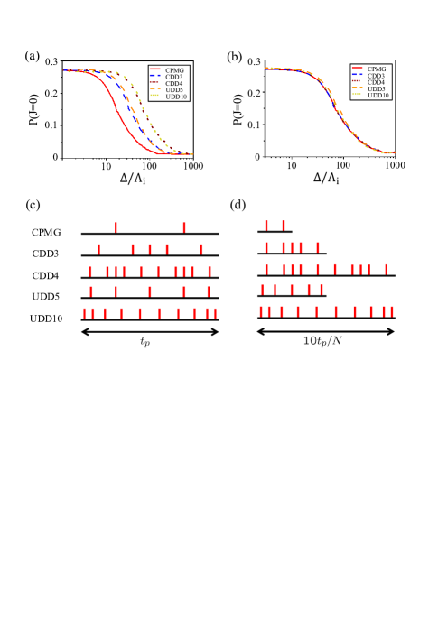
Figure 3: (Color online) Steady state population of many-body singlet $P(J=0)$ versus the strength of inhomogeneous broadening $\Delta$, when the preparation process is protected using different DD pulse sequences. The ensemble consists of 6 qubits, with inhomogeneously broadened energies $\omega_{i}=\Delta(7-2i)/5$, $i=1,2,\ldots,6$. The collective pumping rates are chosen as $\Lambda_{h}=10\Lambda_{i}$ (see text). The red solid, blue dashed, brown dotted, orange dashed, and light yellow dotted curves show numerical results by solving the exact master equation, where the basic unit of the DD control consists of the CPMG, CDD3, CDD4, UDD5 and UDD10 pulse sequences respectively. For the simulation presented in (a), the duration of the basic unit $t_{p}=10^{-3}\Lambda_{i}^{-1}$ for all DD controls compared, as shown in (c). In (b), the duration of the basic unit $t_{p}=10^{-4}\Lambda_{i}^{-1}N$, $N$ being the number of pulses in the basic unit, and the average pulse interval $\bar{\tau}\equiv t_{p}/N$ is taken to be the same for all DD controls compared, as shown in (d).

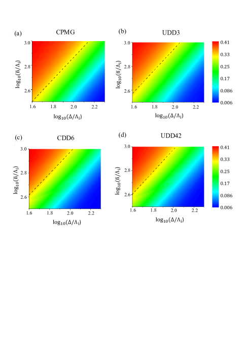
Figure 4: (Color online) Steady state population of many-body singlet $P(J=0)$ as function of the inhomogeneous broadening $\Delta$ and the average pulse density $\bar{n}=N/t_{p}$, where the basic unit of DD control uses various $N$-pulse sequences. The ensemble consists of 6 qubits, with inhomogeneously broadened energies $\omega_{i}=\Delta(7-2i)/5$, $i=1,2,\ldots,6$. The collective pumping rates are chosen as $\Lambda_{h}=100\Lambda_{i}$.

IV DD protection on the dissipative preparation of many-body singlets

In this section, we numerically study the DD protection on an exemplary dissipative state preparation scheme in the presence of inhomogeneous dephasing. The scheme uses collective pumping to prepare many-body singlets 11 . It has been shown that when an ensemble of spins are collectively pumped by the homogeneous collective lowering operator $\sum_{n}\hat{s}_{n}^{-}$ and collective raising operators $\sum_{n}a_{n}\hat{s}_{n}^{+}$ with inhomogeneous coefficients $a_{n}$, the steady state is a highly entangled one in the neighborhood of many-body singlets. In the absence of inhomogeneous and homogeneous dephasing, the singlet population in the steady state $P(J=0)\geq 20\%$. Here we consider the scenario on the preparation of many-body singlet as investigated in Ref. 12 . An spin ensemble with the even number of spins is initially in the fully polarized state. The only two collective pumping operators needed for preparing the many-body singlet from this initial state are respectively $\sum_{n}\hat{s}_{n}^{-}$ and $\sum_{n}(-)^{n}\hat{s}_{n}^{+}$. The preparation channel $\mathcal{L}_{P,0}$ is simply realized by the simultaneous pumping with these two operators, described by the Lindblad form:

$$\mathcal{L}_{P,0}\left[\rho\right]=\sum_{j=1,2}\left[\hat{L}_{j}\rho\hat{L}_{j}^{\dagger}-\frac{1}{2}\left(\rho\hat{L}_{j}^{\dagger}\hat{L}_{j}+\hat{L}_{j}^{\dagger}\hat{L}_{j}\rho\right)\right].$$ (11)

The two Lindblad operators are $\hat{L}_{1}=\sqrt{\Lambda_{h}}\sum_{n}\hat{s}_{n}^{-}$ and $\hat{L}_{2}=\sqrt{\Lambda_{i}}\sum_{n}(-)^{n}\hat{s}_{n}^{+}$, where $\Lambda_{h}$ and $\Lambda_{i}$ characterize the strength of the pumping. In the absence of dephasing noises, the population of many-body singlets $P(J=0)\sim 40\%$ in the steady state when $\Lambda_{h}\gg\Lambda_{i}$ is satisfied. Here, $\Lambda_{i}^{-1}$ characterizes the timescale for reaching the steady state.

In the presence of inhomogeneous broadening in the qubit resonance, the steady state will deviate from the target one because of the inhomogeneous dephasing. We use the population of singlets $P(J=0)$ in the steady state as the figure of merit. To preserve the collective pumping channel while applying the DD control, in the laboratory frame, the Lindblad operators shall alternate between two forms in the even and odd intervals of the DD pulse sequence:

$$\hat{L}_{1}\left(t\right)=\begin{cases}\sqrt{\Lambda_{h}}\sum_{n}\hat{s}_{n}^{-},&\mbox{even interval},\\ \sqrt{\Lambda_{h}}\sum_{n}\hat{s}_{n}^{+}&\mbox{odd interval.}\end{cases}$$ (12)

and

$$\hat{L}_{2}\left(t\right)=\begin{cases}\sqrt{\Lambda_{i}}\sum_{n}(-)^{n}\hat{s}_{n}^{+},&\mbox{even interval},\\ \sqrt{\Lambda_{i}}\sum_{n}(-)^{n}\hat{s}_{n}^{-},&\mbox{odd interval.}\end{cases}$$ (13)

Figure 5: (Color online) Convergence of the Magnus expansion. Solid and dot-dashed curves show the steady state population of many-body singlet $P(J=0)$ obtained by exactly solving the master equation. Dashed and dotted curves are steady state $P(J=0)$ obtained from the Magnus expansion Eq. (3) where we only keep the leading higher order Magnus term (see text). The ensemble consists of 6 qubits, with inhomogeneously broadened energies $\omega_{i}=\Delta(7-2i)/5$, $i=1,2,\ldots,6$. The collective pumping rates are chosen as $\Lambda_{h}=100\Lambda_{i}$. The blue, orange, red and green solid lines represent numerical results when the basic unit of DD control uses the CPMG, UDD3, CDD6 and UDD42 pulse sequences, respectively. The average pulse density is chosen as $\bar{n}\equiv N/t_{p}=10^{2.75}\Lambda_{i}$.

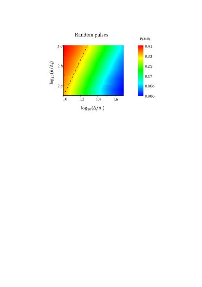
Figure 6: (Color online) Steady state population of the many-body singlet $P(J=0)$ as function of the inhomogeneous broadening $\Delta$ and the average pulse density $\bar{n}=N/t_{p}$ when the DD control uses completely random pulse sequence. The ensemble consists of 6 qubits, with inhomogeneously broadened energies $\omega_{i}=\Delta(7-2i)/5$, $i=1,2,\ldots,6$. The collective pumping rates are chosen as $\Lambda_{h}=100\Lambda_{i}$.

The numerical simulations are shown in Fig. 3 - 6. In Fig. 3, we show the state preparation efficiency with the increase of the inhomogeneous broadening when the preparation process is protected with various pulse sequences. The steady state population of many-body singlet $P(J=0)$ is obtained by solving the master equation exactly. From Fig. 3(a), apparently, the state preparation can tolerate larger inhomogeneous broadening when the basic unit of DD control uses higher order concatenation designs or Uhrig designs when $t_{p}$ is fixed. Interestingly, nearly identical protection efficiencies are observed for CDD3 and UDD5, and also for CDD4 and UDD10. We find the common feature between CDD3 and UDD5, and between CDD4 and UDD10 is that they consist of the same number of $\pi$ pulses. This is consistent with the analysis in section III, namely, the efficiency of protection from inhomogeneous dephasing is largely determined by the density of pulses, rather than the actual design of the sequence. In Fig. 3(c), we compare the performance of various DD controls by fixing the average pulse interval $\bar{\tau}=t_{p}/N$, and different pulse sequences indeed exhibit nearly identical protection efficiency.

In Fig. 4, we examined the protection efficiency as function of both the inhomogeneous broadening and the average pulse density $\bar{n}\equiv 1/\bar{\tau}$. For the four DD controls compared, nearly identical protection efficiency is seen. Moreover, in the double $\log_{10}$ plot, the contour lines are nearly straight lines with slope 1, showing that the strength of the residue noise scales as $\Delta^{2}\bar{\tau}^{2}$. This suggests that $\alpha_{3,b}N^{2}\bar{\tau}^{2}\left[\mathcal{L}_{\mathrm{N}},\left[\mathcal{L}_{\mathrm{P},0},\mathcal{L}_{\mathrm{N}}\right]\right]$ is indeed dominating over other higher order Magnus terms and captures the major effect of the residue noise (c.f. Eq. (10)).

In Fig. 5, we check the convergence of the Magnus expansion by comparing the steady state $P(J=0)$ numerically solved from the exact master equation Eq. (1) with that obtained from the Magnus expansion Eq. (3) where we only keep the leading higher order Magnus term, i.e. by taking $\Omega(t)=t\left(\mathcal{L}_{P,0}+\alpha_{3,b}N^{2}\bar{\tau}^{2}\left[\mathcal{L}_{\mathrm{N}},\left[\mathcal{L}_{\mathrm{P},0},\mathcal{L}_{\mathrm{N}}\right]\right]\right)$. Excellent convergence is found even when the inhomogeneous noise is strong enough to diminish the steady state population of the singlets.

Motivated by the finding that the protection efficiency is determined by the average pulse density and is nearly independent of the pulse structure, we further tested the possibility of protecting the state preparation process by a completely random sequence of $\pi$-pulses. Since the DD control in such case does not have the periodic structure, the analytical results of Eq. (8) and Eq. (9) are no longer applicable. Nevertheless, as shown in Fig. 6, the state preparation can still be well protected from inhomogeneous dephasing. The slope of the contour line is close to 2 in the shown parameter regime, from which we can tell that the residue noise scales as $\Delta^{2}\bar{\tau}$, different from the periodic DD controls where the basic unit uses CPMG, CDD and UDD designs.

Our numerical study shows that sequences of $\pi$ pulses with random arrival times are also efficient in protecting the dissipative state preparation. This means that the protection is insensitive to the errors in the arrival time of the $\pi$ pulses and accurate control on the arrival times is not necessary. The only temporal control needed is that the $\pi$ pulses have to be synchronized with the switches of the pumping operators in the laboratory frame.

V DD protection on the dissipative preparation of linear cluster states

It has also been shown that collective pumping can be used to prepare linear cluster states in an atomic ensemble embedded in a cavity 10 . Here we investigate the DD protection of this dissipative preparation scheme.

Key to the preparation of linear cluster states is to realize the stabilizers through the competition between the optical pumping and the atomic spontaneous emissions. The level scheme for realizing the stabilizer $S_{3}=\hat{s}_{1}^{z}\hat{s}_{2}^{z}\hat{s}_{3}^{z}$ is shown schematically in Fig. 7. The qubit is defined in the ground state manifold $\{|L\rangle_{j},|R\rangle_{j}\}$ of a three level atom. Optical fields denoted by the double head solid lines in Fig. 7 couple the two ground states to the common excited state $|E\rangle_{j}$ with Rabi frequencies $\Omega^{L}_{j}$ and $\Omega^{R}_{j}$ respectively, where $j$ labels the atoms. All atoms are coupled to a common cavity mode with coupling strength $g$. $\Gamma_{j}^{L}$ and $\Gamma_{j}^{R}$ are the spontaneous emission rate from $|E\rangle_{j}$ to the two ground states respectively, whose values are usually considered as the same. Those spontaneous emissions are denoted by wavy lines in Fig. 7. When the driving fields are tuned in resonances with the transitions as indicated in the figure, the eigenstate of stabilizer $S_{3}$ is realized as the steady state of the pumping. Together with single qubit rotations, a complete group of stabilizers for $n-$qubit linear cluster states can be realized one by one (e.g., $S_{4}^{1}=\hat{s}_{1}^{x}\hat{s}_{2}^{z}$, $S_{4}^{2}=\hat{s}_{1}^{z}\hat{s}_{2}^{x}\hat{s}_{3}^{z}$, $S_{4}^{3}=\hat{s}_{2}^{z}\hat{s}_{3}^{x}\hat{s}_{4}^{z}$ and $S_{4}^{4}=\hat{s}_{3}^{z}\hat{s}_{4}^{x}$ for 4-qubit linear cluster states). And thus the fidelity of the linear cluster states can approach unity when damping rate of atomic spontaneous emission $\Gamma$ is much smaller than the cavity-atom coupling strength $g$. More details of the preparation scheme can be found in Ref. 10 .

The scheme relies on delicate engineering of detunings, hence the preparation fidelity will be substantially affected by inhomogeneous broadening of the qubit resonances. We consider interlacing DD pulse sequences with the pumping to suppress the effect of this noise. Since the $\pi-$pulse on the qubit simply switches $|L\rangle_{j}$ and $|R\rangle_{j}$ as to preserve the desired form of pumping channel in the toggling frame, one simply needs to switch values for every pair of Rabi frequencies $\Omega_{j}^{L}$ and $\Omega_{j}^{R}$ and corresponding frequencies of the pump fields in the laboratory frame whenever a $\pi$-pulse is applied in the DD control. The required switching of the controls in the laboratory frame is illustrated in Fig. 7, where part (a) and (b) correspond respectively to the control before and after a $\pi$-pulse is applied. This is equivalent to using different optical pumping fields in the even and odd intervals of the DD control.

In Fig. 8, we show numerical simulation on the protection of preparing a $4$-qubit linear cluster state. The parameters $\Gamma_{j}^{L}=\Gamma_{j}^{R}=0.01g$ and $\Omega_{j}^{L}=\Omega_{j}^{R}=0.01g$. The basic unit of the periodic DD control uses the UDD3 sequence. Indeed, the DD protection is efficient in protecting this dissipative preparation scheme when the inhomogeneous broadening $\Delta\leq 0.1g$. The fidelity of the steady state with the target one approaches unity when the average pulse interval $\bar{\tau}$ is small.

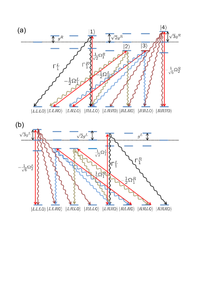
Figure 7: (Color online) Level scheme for realizing the stabilizer $S_{3}=\hat{s}_{1}^{z}\hat{s}_{2}^{z}\hat{s}_{3}^{z}$. In the notations such as $|RLL0\rangle$, the first three letters denote the state of qubit 1, 2, 3 respectively and the last integer denotes the number of cavity photons. The four involved states in the excited state manifold are: $\left|1\right\rangle\equiv 1/\sqrt{2}\left(\left|RLL1\right\rangle+\left|ELL0\right\rangle\right)$, $\left|2\right\rangle\equiv 1/\sqrt{2}\left|RLR1\right\rangle-1/2(\left|ELR0\right\rangle+\left|RLE0\right\rangle)$, $\left|3\right\rangle\equiv 1/\sqrt{2}\left|RRL1\right\rangle-1/2(\left|ERL0\right\rangle+\left|REL0\right\rangle)$, $\left|4\right\rangle\equiv 1/\sqrt{2}\left|RRR1\right\rangle-1/\sqrt{6}(\left|ERR0\right\rangle+\left|RER0\right\rangle+\left|RRE0\right\rangle)$. The wavy lines denote the spontaneous emission. Optical fields resonantly pump the four transitions denoted by the double head solid lines. The eigenstate of stabilizer $S_{3}$ is realized as the steady state of the pumping. (a) and (b) correspond respectively to pumping controls in the laboratory frame before and after a $\pi$ pulse is applied. In (a) the cavity couples to the $\left|R\right\rangle\leftrightarrow\left|E\right\rangle$ transitions with strength $g^{R}$, while in (b) the cavity couples to the the $\left|L\right\rangle\leftrightarrow\left|E\right\rangle$ transitions with strength $g^{L}$ 38 . In the toggling frame, the two pumping controls realize the same dissipative channel.

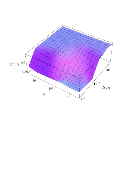
Figure 8: (Color online) Fidelity between the steady state and the target $4$-qubit linear cluster state under the DD protection where the basic unit uses the UDD3 sequence. The inhomogeneously broadened qubit resonances are $\omega_{i}=\Delta(5-2i)/3$, $i=1,2,3,4$. The parameters for the preparation channel are: $\Omega_{j}^{L}=\Omega_{j}^{R}=0.01g$, $\Gamma_{j}^{L}=\Gamma_{j}^{R}=0.01g$. See text.

VI DD Protection from dynamic noises

Dynamic fluctuation in the environment can also lead to qubit dephasing. Here we investigate the possibility of DD protection of the dissipative state preparation in the presence of dynamic noise, for which we assume a semiclassical form. The qubit energies are given by $H_{\mathrm{SC}}=\sum_{i}B_{i}\left(t\right)\sigma_{i}^{z}$, where $B_{i}(t)$ is stochastic and is characterized by the autocorrelation functions $\left\langle B_{i}\left(t\right)B_{j}\left(t^{\prime}\right)\right\rangle=G\left(t-t^{\prime}\right)\delta_{i,j}$. We further assume the noises are Gaussian, for which we can derive the Kubo stochastic Liouville equation 39 in the toggling frame as

$$\dot{\rho}=\mathcal{L}_{\mathrm{P,0}}\left[\rho\right]+\mathcal{L}_{\mathrm{N}}^{\mathrm{eff}}\left[t;\rho\right]$$ (14)

where the effective noise operator is

$$\mathcal{L}_{\mathrm{N}}^{\mathrm{eff}}\left[t;\rho\right]=\sum_{i}\int_{0}^{t}dt_{1}G\left(t-t_{1}\right)f(t)f(t_{1})\mathcal{L}^{i}\left(t-t_{1}\right)$$ (15)

with $\mathcal{L}^{i}\left(t\right)=\mathcal{L}_{\mathrm{V}}^{i}\mathcal{\widetilde{L}}_{\mathrm{V}}^{i}\left(t\right)$, where $\mathcal{L}_{\mathrm{V}}^{i}\left[\rho\right]=-i\left[\sigma_{i}^{z},\rho\right]$ and $\mathcal{\widetilde{L}}_{\mathrm{V}}^{i}\left(t\right)=\exp\left(\mathcal{L}_{\mathrm{P,0}}t\right)\mathcal{L}_{\mathrm{V}}^{i}\exp\left(-\mathcal{L}_{\mathrm{P,0}}t\right)$. $f(t)=(-)^{i}$ for $\tau_{i}<t<\tau_{i+1}$ is the step-like function corresponding to the DD control.

Following Eq. (4a), the first term of the Magnus series can be written as

$$\Omega_{1}\left(t\right)=t\mathcal{L}_{\mathrm{P,0}}\left[\rho\right]+\int_{0}^{\infty}G\left(\omega\right)\left|F\left(\omega,t\right)\right|d\omega,$$ (16)

where $G\left(\omega\right)=1/2\pi\int_{-\infty}^{\infty}G\left(t\right)\exp(-i\omega t)dt$ is the noise spectrum, and $F$ is the filter function corresponding to the DD control used 30 ; 40 ; 41 ; 42

$$\left|F\left(\omega,t\right)\right|=\sum_{i}\int_{0}^{t}\int_{0}^{t_{1}}\frac{dt_{1}dt_{2}}{2\pi}f(t_{1})f(t_{1}-t_{2})\cos\omega t_{2}\mathcal{L}^{i}\left(t_{2}\right).$$ (17)

In the case of protecting quantum memory, the preparation channel $\mathcal{L}_{\mathrm{P,0}}$ is absent. Thus $\mathcal{L}^{i}\left(t_{2}\right)=\left(\mathcal{L}_{\mathrm{V}}^{i}\right)^{2}$, which is time-independent and can be taken out of the integral in Eq. (17). In such case, concatenated DD or Uhrig DD pulse sequences can generate the filter function that suppresses dynamic noise to arbitrarily high order of pulse intervals 30 ; 40 ; 41 ; 42 .

However, for the protection of a dissipative state preparation, because of the presence of the nontrivial preparation channel $\mathcal{L}_{\mathrm{P,0}}$, $\mathcal{L}^{i}\left(t_{2}\right)$ can be time-dependent due to the interference between $\mathcal{L}_{\mathrm{P,0}}$ and $\mathcal{L}_{\mathrm{V}}^{i}$. The effect of dynamics noises can not be arbitrarily suppressed as in the case of DD protection of quantum memory. In general, $F$ scales as $\bar{\tau}^{2}$, and the dynamical noise can be suppressed to the second-order of the pulse interval.

VII Summary

We investigated the protection of dissipative quantum state preparation processes against qubit dephasing by interlacing the DD control pulse sequences with the preparation control. The basic idea is to average out the noise channels over time, while preserving the irreversible dynamics for generating desired entanglement in the steady state. By utilizing DD control consisting of sequences of short $\pi$-pulses, the dephasing noise can be suppressed to certain order of pulse interval and thus high-fidelity state preparation can be realized when the DD control has sufficiently small pulse interval. With the help of generalized Magnus series, we investigated the order of suppression of noise channels. For inhomogeneous dephasing, the leading noise term in the Magnus expansion is of second order of the pulse interval, and is largely determined by the average pulse interval rather than the types of DD control sequences used. The DD protection efficiency is demonstrated by numerical simulations on two exemplary state preparation schemes for realizing many-body singlets and linear cluster states respectively. DD protection from dynamical noise is discussed for the example of Gaussian noise of a semiclassical description, where the leading noise effect is also of second order of the pulse interval.

- (1) S. Clark, A. Peng, M. Gu, and S. Parkins, Phys. Rev. Lett. 91, 177901 (2003).
- (2) S. Schneider and G. J. Milburn, Phys. Rev. A 65, 042107 (2002).
- (3) M. Paternostro, W. Son, and M. S. Kim, Phys. Rev. Lett. 92, 197901 (2004).
- (4) M. J. Kastoryano, F. Reiter, and A. S. Sørensen, Phys. Rev. Lett. 106, 090502 (2011).
- (5) F. Verstraete, M. M. Wolf, and J. I. Cirac, Nat. Phys. 5, 633 (2009).
- (6) S. Diehl, A. Micheli, A. Kantian, B. Kraus, H. P. Bü chler, and P. Zoller, Nat. Phys. 4, 878 (2008).
- (7) B. Kraus, H. P. Büchler, S. Diehl, A. Kantian, A. Micheli, and P. Zoller, Phys. Rev. A 78, 042307 (2008).
- (8) H. Krauter, C. A. Muschik, K. Jensen, W. Wasilewski, J. M. Petersen, J. I. Cirac, and E. S. Polzik, Phys. Rev. Lett. 107, 080503 (2011).
- (9) H. Weimer, M. Müller, I. Lesanovsky, P. Zoller and H. P. Büchler, Nat. Phys. 6, 382 (2010).
- (10) J. Cho, S. Bose, and M. S. Kim, Phys. Rev. Lett. 106, 020504 (2011).
- (11) W. Yao, Phys. Rev. B 83, 201308(R) (2011).
- (12) H.-Y. Yu, Y. Luo, and W. Yao, Phys. Rev. A 84, 032337 (2011).
- (13) Y. Luo, H.-Y. Yu, and W. Yao, Phys. Rev. B 85, 155304 (2012).
- (14) D. Gottesman and I. L. Chuang, Nature 402, 390 (1999).
- (15) M. Murao, D. Jonathan, M. B. Plenio, and V. Vedral, Phys. Rev. A 59, 156 (1999).
- (16) R. Raussendorf and H. J. Briegel, Phys. Rev. Lett. 86, 5188 (2001).
- (17) H. J. Briegel, D. E. Browne,W. Dür, R. Raussendorf and M. Van den Nest, Nat. Phys. 5, 19 (2009).
- (18) E. L. Hahn, Phys. Rev. 80, 580 (1950).
- (19) M. Mehring, Principles of High Resolution NMR in Solids (Spinger-Verleg, Berlin, 1983), 2nd ed.
- (20) W.-K. Rhim, A. Pines, and J. S. Waugh, Phys. Rev. Lett. 25, 218 (1970).
- (21) U. Haeberlen, High resolution NMR in solids: selective averaging (Academic Press, New York, 1976).
- (22) L. Viola and S. Lloyd, Phys. Rev. A 58, 2733 (1998).
- (23) M. Ban, J. Mod. Opt. 45, 2315 (1998).
- (24) P. Zanardi, Phys. Lett. A 258, 77 (1999).
- (25) L. Viola, E. Knill, and S. Lloyd, Phys. Rev. Lett. 82, 2417 (1999).
- (26) D. A. Lidar, Phys. Rev. Lett. 100, 160506 (2008).
- (27) C. Barthel, J. Medford, C. M. Marcus, M. P. Hanson, and A. C. Gossard, Phys. Rev. Lett. 105, 266808 (2010).
- (28) T. van der Sar, Z. H. Wang, M. S. Blok, H. Bernien, T. H. Taminiau, D. M. Toyli, D. A. Lidar, D. D. Awschalom, R. Hanson, and V. V. Dobrovitski, Nature 484, 82 (2012).
- (29) J. R. West, D. A. Lidar, B. H. Fong, and M. F. Gyure, Phys. Rev. Lett. 105, 230503 (2010).
- (30) X. K. Xu, Z. X. Wang, C. K. Duan, P. Huang, P. F. Wang, Y. Wang, N. Y. Xu, X. Kong, F. Z. Shi, X. Rong, and J. F. Du, Phys. Rev. Lett. 109, 070502 (2012).
- (31) H. Carr and E. M. Purcell, Phys. Rev. 94, 630 (1954).
- (32) S. Meiboom and D. Gill, Rev. Sci. Instrum. 29, 688 (1958).
- (33) K. Khodjasteh and D. A. Lidar, Phys. Rev. Lett. 95, 180501 (2005).
- (34) K. Khodjasteh and D. A. Lidar, Phys. Rev. A 75, 062310 (2007).
- (35) W. Yao, R. B. Liu, and L. J. Sham, Phys. Rev. Lett. 98, 077602 (2007).
- (36) R. B. Liu, W. Yao, and L. J. Sham, New J. Phys. 9, 226 (2007).
- (37) W. M. Witzel and S. Das Sarma, Phys. Rev. B 76, 241303(R) (2007).
- (38) W. X. Zhang, V. V. Dobrovitski, L. F. Santos, L. Viola, and B. N. Harmon, Phys. Rev. B 75, 201302(R) (2007).
- (39) G. S. Uhrig, Phys. Rev. Lett. 98, 100504 (2007).
- (40) B. Lee, W. M. Witzel, and S. Das Sarma, Phys. Rev. Lett. 100, 160505 (2008).
- (41) G. S. Uhrig, New J. Phys. 10, 083024 (2008).
- (42) W. Yang and R.-B. Liu, Phys. Rev. Lett. 101, 180403 (2008).
- (43) L. Viola and E. Knill, Phys. Rev. Lett. 94, 060502 (2005).
- (44) L. F. Santos and L. Viola, Phys. Rev. Lett. 97, 150501 (2006).
- (45) S. Blanes, F. Casas, J. A. Oteo, and J. Ros, Phys. Rep. 470, 151 (2009).
- (46) Such tunable cavity-atom couplings are required by the original proposal in Ref. 10 .
- (47) R. Kubo, J. Math. Phys. 4, 174 (1963).
- (48) A. G. Kofman and G. Kurizki, Phys. Rev. Lett. 93, 130406 (2004).
- (49) H. Uys, M. J. Biercuk, and J. J. Bollinger, Phys. Rev. Lett. 103, 040501 (2009).
- (50) Ł. Cywiński, R. M. Lutchyn, C. P. Nave, and S. Das Sarma, Phys. Rev. B 77, 174509 (2008).