Delta-N Formalism for Curvaton with Modulated Decay

Abstract

In this paper, the curvature perturbation generated by the modulated curvaton decay is studied by a direct application of $\delta N$-formalism. Our method has a sharp contrast with the non-linear formalism which may be regarded as an indirect usage of $\delta N$-formalism. We first show that our method can readily reproduce results in previous works of modulation of curvaton. Then we move on to calculate the case where the curvaton mass (and hence also the decay rate) is modulated. The method can be applied to the calculation of the modulation in the freezeout model, in which the heavy species are considered instead of the curvaton. Our method explains curvaton and various modulation on an equal footing.

I Introduction

It is widely believed that a stage of cosmic inflation Lyth:2009zz which happens in the very early universe is necessary to explain the primordial curvature perturbation. During inflation the quantum fluctuations of light scalar fields are expanded to become superhorizon classical fluctuations. One or more of those field fluctuations are supposed to be responsible for the curvature perturbation; the field may not be the inflaton field which drives inflation, but the curvaton field $\sigma$ Lyth:2001nq ; Enqvist:2001zp ; Moroi:2001ct or the modulation field $\chi$ Dvali:2003em ; Kofman:2003nx ; Dvali:2003ar which modulates the decay rate of the inflaton field.

According to the $\delta N$-formalism Sasaki:1995aw ; Sasaki:1998ug ; Lyth:2004gb ; Lyth:2005fi (see also Kodama:1997qw ), the curvature perturbation resulted from a field $\phi$ is given by

$$\zeta=\delta N=N_{\phi}\delta\phi+\frac{1}{2}N_{\phi\phi}(\delta\phi)^{2}+\frac{1}{6}N_{\phi\phi\phi}(\delta\phi)^{3}+\cdots,$$ (1)

where $N=\int d\ln a$ is the number of e-folds and $a$ denotes the scale factor. The spectrum of the perturbation is ${\cal P}_{\delta\phi}^{1/2}\sim H/2\pi$ at the horizon exit. Here $\phi$ may be the conventional inflaton field ($\varphi$), the curvaton field ($\sigma$) or the modulation field ($\chi$) which are light (compared with the Hubble parameter) during inflation. The fluctuations of those fields can (eventually) affect $N$. The subscript means derivative with respect to $\phi$. Note that $\delta\phi$ is calculated on a flat slice (gauge) and $\zeta$ is defined to be the curvature perturbation on uniform energy density slice. It is convenient to estimate the magnitude of the higher order effects by using the nonlinear parameters $f_{NL}$ and $g_{NL}$ defined by

$$\zeta=\zeta_{g}+\frac{3}{5}f_{NL}\zeta^{2}_{g}+\frac{9}{25}g_{NL}\zeta^{3}_{g}+\cdots,$$ (2)

where $\zeta_{g}=N_{\phi}\delta\phi$ denotes the Gaussian (i.e, the first-order expansion with respect to the Gaussian perturbation $\delta\phi$) part of $\zeta$. From Eq. (1) we can see that

$$f_{NL} = \frac{5}{6}\frac{N_{\phi\phi}}{(N_{\phi})^{2}},$$ (3)

$$g_{NL} = \frac{25}{54}\frac{N_{\phi\phi\phi}}{(N_{\phi})^{3}}.$$ (4)

Current experimental data gives (very) roughly Bennett:2012fp ; Smidt:2010sv

$$|f_{NL}| \lesssim 100,$$ (5)

$$|g_{NL}| \lesssim 10^{6}.$$ (6)

In the near future, the PLANCK satellite is expected to reduce the bound to $|f_{NL}|\lesssim 10$ and $|g_{NL}|\lesssim 10^{5}$ Smidt:2010ra if non-gaussianity is not detected.

In some recent works the question of combining curvaton and inhomogeneous reheating scenarios has been studied in the light of the modulated curvaton decay Enomoto:2012uy ; Langlois:2013dh ; Assadullahi:2013ey ; Enomoto:2013qf , where the non-linear formalism of the component perturbations based on Lyth:2004gb , has been used.

In this paper, we propose a direct method which is conceptually simple and straightforward. In section II, we show that the method can be used to produce previous results of Langlois:2013dh ; Assadullahi:2013ey ; Enomoto:2013qf , in which non-linear formalism has been used. In section III, in addition to the modulated decay rate, we consider the modulation caused by the modulated curvaton mass. In appendix A.1, we compare the calculation in section II and section III. In appendix A.2, we reproduce standard formulas for the conventional curvaton. In section IV, the modulation in the freezeout model Dvali:2003ar is solved when the massive species might not dominate the density. Our method explains the curvaton model and the various modulation scenarios on an equal footing.

II Modulated decay rate of the curvaton model : unmodulated mass

In this section, we will calculate the curvature perturbation when the curvaton decay is modulated. We consider the case in which the decay rate is modulated by a light scalar field $\chi$ through a coupling. The case of the modulated decay rate through a mass is considered in the next section.

Consider a curvaton field $\sigma$ with a quadratic potential $V(\sigma)=(1/2)m^{2}\sigma^{2}$. The number of e-folds between curvaton oscillation $a_{o}$ to a uniform energy density time slice after curvaton decay at $a_{c}$, is given by

$$N=\ln\left(\frac{a_{c}}{a_{o}}\right)=\ln\left(\frac{a_{d}}{a_{o}}\right)+\ln\left(\frac{a_{c}}{a_{d}}\right)\equiv N_{1}+N_{2},$$ (7)

where $a_{d}$ represents curvaton decay at $H\sim\Gamma$ and the two parts are denoted by $N_{1}$ and $N_{2}$, respectively. After curvaton decay the universe is dominated by radiation therefore $H\propto a^{-2}$ and we can write $N_{2}$ as

$$N_{2}=\frac{1}{2}\ln\left(\frac{\Gamma}{H(a_{c})}\right),$$ (8)

where we have used $H(a_{d})=\Gamma$ and $H(a_{c})$ corresponds to the uniform energy density slice (which does not depend on $\sigma$ or $\chi$). See also Fig.1.

By definition of the oscillating curvaton, when the curvaton start to oscillate some time after inflation when $H\sim m$ at $a_{o}$, the energy density is dominated by radiation $\gamma$. The energy densities are hence given by $\rho_{o}\sim\rho_{o,\gamma}=3m^{2}M_{p}^{2}$ and $\rho_{o,\sigma}=(1/2)m^{2}\sigma^{2}$. Here the reduced Planck mass is $M_{p}=2.4\times 10^{18}\mbox{ GeV}$ and $\sigma$ denotes the field value of the curvaton when it starts to oscillate. On the other hand, at curvaton decay ($H\sim\Gamma$) the energy densities are given by $\rho_{d}=3\Gamma^{2}M_{p}^{2}$ and $\rho_{d,\sigma}=(1/2)m^{2}\sigma(t_{o})^{2}(a_{d}/a_{o})^{-3}$ because the curvaton behaves like cold matter during oscillation.

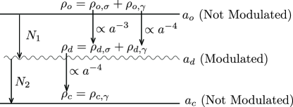
Figure 1: The modulated decay in the curvaton model is illustrated. The curvaton density at $a_{o}$ is $\rho_{o,\sigma}=\frac{1}{2}m^{2}\sigma^{2}\ll\rho_{o,\gamma}$, which gives the curvaton density at the decay $\rho_{d,\sigma}=\rho_{o,\sigma}X^{-3}$ where $X\equiv(a_{d}/a_{o})$.

If we focus on radiation (which dilutes as $a^{-4}$) during this period and define $X\equiv(a_{d}/a_{o})$ for notational simplicity, we can write

$$X^{4}\equiv\frac{\rho_{o,\gamma}}{\rho_{d,\gamma}}=\frac{3m^{2}M_{p}^{2}}{3\Gamma^{2}M_{p}^{2}-\frac{m^{2}\sigma^{2}}{2X^{3}}},$$ (9)

or

$$3\Gamma^{2}M_{p}^{2}X^{4}-\frac{1}{2}m^{2}\sigma^{2}X=3m^{2}M_{p}^{2}.$$ (10)

For later usage, we define a quantity $r$ used widely in literatures of curvaton by

$$r\equiv\frac{3\rho_{d,\sigma}}{4\rho_{d,\gamma}+3\rho_{d,\sigma}}=\frac{3\left(\frac{1}{2}m^{2}\sigma^{2}\right)X^{-3}}{4\left[3\Gamma^{2}M_{p}^{2}-\left(\frac{1}{2}m^{2}\sigma^{2}\right)X^{-3}\right]+3\left(\frac{1}{2}m^{2}\sigma^{2}\right)X^{-3}}=\frac{3(\frac{1}{2}m^{2}\sigma^{2})}{12\Gamma^{2}M_{p}^{2}X^{3}-\frac{1}{2}m^{2}\sigma^{2}}.$$ (11)

In the oscillating curvaton model, $r$ is comparable to the ratio of the curvaton energy density to the total energy density of the Universe at the curvaton decay.

The modulated curvaton decay is introduced by the function $\Gamma(\chi)$, which becomes inhomogeneous in space due to the modulation caused by a light field $\chi$. From Eq. (1), the curvature perturbation to linear order is given by $\zeta=N_{\chi}\delta\chi+...$, where other sources (e.g, inflaton perturbation $\delta\varphi$ and the conventional curvaton perturbation $\delta\sigma$) are included in “…”. The last expression in Eq. (11) is convenient because it allows us to calculate the derivatives of r with respect to the fields. A very simple but handy relation which will be used frequently in this paper is

$$\frac{12\Gamma^{2}M_{p}^{2}X^{3}}{12\Gamma^{2}M_{p}^{2}X^{3}-\frac{1}{2}m^{2}\sigma^{2}}=\frac{12\Gamma^{2}M_{p}^{2}X^{3}-\frac{1}{2}m^{2}\sigma^{2}+\frac{1}{2}m^{2}\sigma^{2}}{12\Gamma^{2}M_{p}^{2}X^{3}-\frac{1}{2}m^{2}\sigma^{2}}=1+\frac{r}{3}.$$ (12)

By making derivative of both sides of Eq. (10) with respect to $\chi$, we obtain

$$6\Gamma\Gamma_{\chi}M_{p}^{2}X^{4}+12\Gamma^{2}M_{p}^{2}X^{3}X_{\chi}-\frac{1}{2}m^{2}\sigma^{2}X_{\chi}=0,$$ (13)

which implies

$$N_{1\chi} \equiv \frac{\partial N_{1}}{\partial\chi}=(\ln X)_{\chi}=\frac{X_{\chi}}{X}$$ (14)

$$= \frac{6\Gamma^{2}M_{p}^{2}X^{3}}{\frac{1}{2}m^{2}\sigma^{2}-12\Gamma^{2}M_{p}^{2}X^{3}}\frac{\Gamma_{\chi}}{\Gamma}$$

$$= -\left(\frac{1}{2}+\frac{r}{6}\right)\frac{\Gamma_{\chi}}{\Gamma},$$

where Eq. (12) has been used.

$N_{2\chi}$ is evaluated by making a derivate of Eq. (8):

$$N_{2\chi}\equiv\frac{\partial N_{2}}{\partial\chi}=\frac{1}{2}\frac{\Gamma_{\chi}}{\Gamma}.$$ (15)

Therefore we have

$$N_{\chi}=N_{1\chi}+N_{2\chi}=-\frac{1}{6}r\frac{\Gamma_{\chi}}{\Gamma}.$$ (16)

This gives for example, Eq. (31) in Enomoto:2013qf and also consistent with Langlois:2013dh and Assadullahi:2013ey .

It is also straightforward to calculate the non-linear parameters. By making derivative of Eq. (16) once more we have

$$N_{\chi\chi}=\frac{r_{\chi}}{r}N_{\chi}-\frac{1}{6}r\left(\frac{\Gamma_{\chi\chi}\Gamma-\Gamma_{\chi}^{2}}{\Gamma^{2}}\right).$$ (17)

In order to evaluate $r_{\chi}\equiv\partial r/\partial\chi$, we make derivative of $r$ by using the last expression in Eq. (11) and keep in mind that $\Gamma(\chi)$ and $X(\chi)$ are now functions of $\chi$. We have

$$r_{\chi} = \frac{-3\left(\frac{1}{2}m^{2}\sigma^{2}\right)}{12\Gamma^{2}X^{3}-\frac{1}{2}m^{2}\sigma^{2}}\frac{24\Gamma\Gamma_{\chi}X^{3}+36\Gamma^{2}X^{2}X_{\chi}}{12\Gamma^{2}X^{3}-\frac{1}{2}m^{2}\sigma^{2}}$$ (18)

$$= -r\left[2\left(1+\frac{r}{3}\right)\frac{\Gamma_{\chi}}{\Gamma}+3\left(1+\frac{r}{3}\right)\frac{X_{\chi}}{X}\right],$$

where we have used Eq. (12) to obtain the second equality. From Eq. (16) and (14) we find useful relations

$$\frac{\Gamma_{\chi}}{\Gamma} = -\frac{6}{r}N_{\chi}$$

$$\frac{X_{\chi}}{X} = \left(\frac{3}{r}+1\right)N_{\chi}.$$ (19)

By using these relations we obtain

$$\frac{r_{\chi}}{r}=\frac{3-2r-r^{2}}{r}N_{\chi}.$$ (20)

Therefore we find

$$\frac{6}{5}f_{NL}=\frac{N_{\chi\chi}}{N_{\chi}^{2}}=\frac{3}{r}\left(3-2\frac{\Gamma\Gamma_{\chi\chi}}{\Gamma_{\chi}^{2}}\right)-2-r=\left[\frac{9}{r}-2-r\right]-\frac{6}{r}\left(\frac{\Gamma\Gamma_{\chi\chi}}{\Gamma_{\chi}^{2}}\right).$$ (21)

By taking derivative of Eq. (98) with respect to $\chi$, we have

$$N_{\chi\sigma}=\frac{2}{3}\frac{r_{\chi}}{\sigma}=-\frac{r(1-r)(3+r)\Gamma_{\chi}}{9\Gamma\sigma},$$ (22)

where Eq. (20) has been used to evaluate $r_{\chi}$. Therefore by using Eqs. (16) and (98) we can obtain

$$\frac{6}{5}f^{\sigma\chi}_{NL}\equiv\frac{N_{\chi\sigma}}{N_{\chi}N_{\sigma}}=\frac{(1-r)(3+r)}{r}.$$ (23)

We can carry on to calculate $g_{NL}$. Firstly we substitute Eq. (20) into Eq. (17) to write

$$N_{\chi\chi}=\frac{3-2r-r^{2}}{r}N_{\chi}^{2}-\frac{1}{6}r\left(\frac{\Gamma_{\chi\chi}\Gamma-\Gamma_{\chi}^{2}}{\Gamma^{2}}\right),$$ (24)

and making derivative with respect to $\chi$ once more. Then eliminate $r_{\chi}$ again by Eq. (20), finally we obtain

$$\frac{54}{25}g_{NL} = \frac{N_{\chi\chi\chi}}{N_{\chi}^{3}}$$ (25)

$$= \frac{1}{r^{2}}\left[135-54r-22r^{2}+10r^{3}+3r^{4}-18\left(9-2r-r^{2}\right)\frac{\Gamma\Gamma_{\chi\chi}}{\Gamma_{\chi}^{2}}+36\frac{\Gamma_{\chi\chi\chi}\Gamma^{2}}{\Gamma_{\chi}^{3}}\right].$$

This gives Eq. (43) in Assadullahi:2013ey and Eq. (28) in Langlois:2013dh . It should be clear that our method is capable to reproduce previous results.

III Modulated decay rate of the curvaton model : modulated mass

In this section, we apply our method to the case where the modulated decay rate is sourced by the modulated curvaton mass. This is more complicated than the previous case because now the time slice when the curvaton start to oscillate is also modulated. In that way, the quantities defined at $a_{o}$ may also depend on $\chi$. We thus need to introduce $a_{i}$ before $a_{o}$, since not only $a_{d}$ but also $a_{o}$ is modulated. See also Fig.2

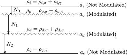
Figure 2: The modulated decay in the curvaton model is illustrated when the curvaton mass is modulated.

Before the curvaton oscillation, the curvaton is slow-rolling and we assume that the curvaton density is scaling like $\rho_{\sigma}\propto a^{-\epsilon_{w}}$ just before the oscillation. In general $\epsilon_{w}$ is time-dependent in the radiation-dominated Universe; however for the modulation at $a_{0}$ we only need $\epsilon_{w}$ defined very close to $a_{o}$. Therefore in our calculation we can assume that $\epsilon_{w}$ is approximately a constant.

The e-folding number is now given by

$$N=\ln\left(\frac{a_{c}}{a_{i}}\right)=\ln\left(\frac{a_{o}}{a_{i}}\right)+\ln\left(\frac{a_{d}}{a_{o}}\right)+\ln\left(\frac{a_{c}}{a_{d}}\right)=N_{0}+N_{1}+N_{2},$$ (26)

where $N_{2}$ is again given by Eq. (8) and $N_{2\chi}$ is given by Eq. (15).

In order to calculate $N_{0\chi}$, we set the fraction of the energy density at $a_{i}$ as

$$f_{i}\equiv\frac{\rho_{i,\sigma}}{\rho_{i}}=\frac{\rho_{i,\sigma}}{3H^{2}_{i}M_{p}^{2}}.$$ (27)

If we define

$$N_{0}=\ln\left(\frac{a_{o}}{a_{i}}\right)\equiv\ln X_{0},$$ (28)

we find

$$X_{0}^{4}=\frac{\rho_{i,\gamma}}{\rho_{o,\gamma}}=\frac{3H_{i}^{2}(1-f_{i})}{3m^{2}(1-f_{o})},$$ (29)

where

$$f_{o} \equiv \frac{\rho_{o,\sigma}}{3m^{2}M_{p}^{2}}=\frac{\rho_{i,\sigma}X_{0}^{-\epsilon_{w}}}{3m^{2}M_{p}^{2}}$$

$$\frac{\partial f_{o}}{\partial\chi}=-\left(\epsilon_{w}\frac{X_{0\chi}}{X_{0}}\right)f_{o}$$

$$f_{i} \equiv \frac{\rho_{i,\sigma}}{\rho_{i}}=\frac{\rho_{i,\sigma}}{3H^{2}_{i}M_{p}^{2}}$$ (30)

$$\frac{\partial f_{i}}{\partial\chi}=2\frac{m_{\chi}}{m}f_{i}.$$

Here, for the curvaton density we assume $\rho_{i,\sigma}\propto m^{2}$. We can find from Eq.(29):

$$4X_{0}^{3}X_{0\chi}=-\frac{\partial f_{i}}{\partial\chi}\frac{\rho_{i}}{\rho_{o,\gamma}}-2\frac{m_{\chi}}{m}\frac{\rho_{i,\gamma}}{\rho_{o,\gamma}}+\frac{\partial f_{o}}{\partial\chi}\frac{\rho_{i,\gamma}\rho_{o}}{\rho_{o,\gamma}^{2}}.$$ (31)

Considering $\frac{\rho_{i,\gamma}}{\rho_{o,\gamma}}=X_{0}^{4}$, we find

$$4\frac{X_{0\chi}}{X_{0}} = -2\frac{m_{\chi}}{m}\frac{(\rho_{i}f_{i})}{\rho_{i,\gamma}}-2\frac{m_{\chi}}{m}-\epsilon_{w}\frac{X_{0\chi}}{X_{0}}\frac{(\rho_{o}f_{o})}{\rho_{o,\gamma}}.$$ (32)

Solving that equation for $\frac{X_{0\chi}}{X_{0}}$, we obtain

$$\frac{X_{0\chi}}{X_{0}} = -\frac{1}{2}(1-r_{o})\frac{m_{\chi}}{m}\left(1+\frac{\rho_{i,\sigma}}{\rho_{i,\gamma}}\right),$$ (33)

where

$$r_{o} \equiv \frac{\epsilon_{w}\rho_{o,\sigma}}{4\rho_{o,\gamma}+\epsilon_{w}\rho_{o,\sigma}}$$

$$(1-r_{o}) \equiv \frac{4\rho_{o,\gamma}}{4\rho_{o,\gamma}+\epsilon_{w}\rho_{o,\sigma}}.$$ (34)

Finally, we have

$$N_{0\chi} = (\ln X_{0})_{\chi}$$ (35)

$$= -\frac{1}{2}(1-r_{o})\frac{m_{\chi}}{m}\left(1+\frac{\rho_{i,\sigma}}{\rho_{i,\gamma}}\right).$$

For the usual set-ups $f_{i}\simeq f_{o}\simeq 0$, the result shows

$$N_{0\chi}\simeq-\frac{1}{2}\frac{m_{\chi}}{m}.$$ (36)

For the second stage (i.e, during the curvaton oscillation), we define

$$N_{1}=\ln\left(\frac{a_{d}}{a_{o}}\right)=\ln X_{1}.$$ (37)

Then

$$X_{1}^{4}=\frac{\rho_{o,\gamma}}{\rho_{d,\gamma}}=\frac{3m^{2}(1-f_{o})}{3\Gamma^{2}(1-f_{d})},$$ (38)

where

$$f_{d} \equiv \frac{\rho_{d,\sigma}}{\rho_{d}}=\frac{\rho_{i,\sigma}X_{1}^{-3}X_{o}^{-\epsilon_{w}}}{3\Gamma^{2}M_{p}^{2}}$$

$$\frac{\partial f_{d}}{\partial\chi}=\left(-3\frac{X_{1\chi}}{X_{1}}-\epsilon_{w}\frac{X_{0\chi}}{X_{0}}+2\frac{m_{\chi}}{m}-2\frac{\Gamma_{\chi}}{\Gamma}\right)f_{d}$$

$$f_{o} \equiv \frac{\rho_{o,\sigma}}{\rho_{o}}=\frac{\rho_{i,\sigma}X_{0}^{-\epsilon_{w}}}{3m^{2}M_{p}^{2}}$$ (39)

$$\frac{\partial f_{o}}{\partial\chi}=\left(-\epsilon_{w}\frac{X_{0\chi}}{X_{0}}\right)f_{o}.$$

We thus find from Eq.(38):

$$4X_{1}^{3}X_{1\chi}=\left(2\frac{m_{\chi}}{m}-2\frac{\Gamma_{\chi}}{\Gamma}\right)\frac{\rho_{o,\gamma}}{\rho_{d,\gamma}}-\frac{\partial f_{o}}{\partial\chi}\frac{\rho_{o}}{\rho_{d,\gamma}}+\frac{\partial f_{d}}{\partial\chi}\frac{\rho_{o,\gamma}\rho_{d}}{\rho_{d,\gamma}^{2}}.$$ (40)

By using $\frac{\rho_{o,\gamma}}{\rho_{d,\gamma}}=X_{1}^{4}$, we find

$$4\frac{X_{1\chi}}{X_{1}} = \left(2\frac{m_{\chi}}{m}-2\frac{\Gamma_{\chi}}{\Gamma}\right)-\epsilon_{w}\frac{X_{o\chi}}{X_{0}}\frac{(\rho_{o}f_{o})}{\rho_{o,\gamma}}+\left(-3\frac{X_{1\chi}}{X_{1}}-\epsilon_{w}\frac{X_{0\chi}}{X_{0}}+2\frac{m_{\chi}}{m}-2\frac{\Gamma_{\chi}}{\Gamma}\right)\frac{(\rho_{d}f_{d})}{\rho_{d,\gamma}}.$$ (41)

Although not mandatory, we are going to assume $\epsilon_{w}\ll 1$ in this paper. Solving the equation for $\frac{X_{1\chi}}{X_{1}}$, we find

$$\frac{X_{1\chi}}{X_{1}} \simeq -\frac{2(\rho_{d,\gamma}+\rho_{d,\sigma})}{4\rho_{d,\gamma}+3\rho_{d,\sigma}}\ \left(\frac{\Gamma_{\chi}}{\Gamma}-\frac{m_{\chi}}{m}\right)$$ (42)

$$= -\left(\frac{1}{6}r+\frac{1}{2}\right)\left(\frac{\Gamma_{\chi}}{\Gamma}-\frac{m_{\chi}}{m}\right).$$

where $r$ is given by Eq. (11) and we have used the relation

$$\frac{1}{6}r+\frac{1}{2}=\frac{2\rho_{d,\gamma}+2\rho_{d,\sigma}}{4\rho_{d,\gamma}+3\rho_{d,\sigma}}=\frac{2\rho_{d}}{4\rho_{d,\gamma}+3\rho_{d,\sigma}}.$$ (43)

Therefore

$$N_{1\chi} = (\ln X_{1})_{\chi}$$ (44)

$$\simeq -\left(\frac{1}{6}r+\frac{1}{2}\right)\left(\frac{\Gamma_{\chi}}{\Gamma}-\frac{m_{\chi}}{m}\right).$$

Our final result is

$$N_{\chi} = N_{0\chi}+N_{1\chi}+N_{2\chi}$$ (45)

$$\simeq \frac{r}{6}\left[-\frac{\Gamma_{\chi}}{\Gamma}+\frac{m_{\chi}}{m}\right]$$ (46)

To understand the result, imagine an explicit form of $\Gamma$. Just for instance, one may assume $\Gamma\propto\lambda m^{n}$. This gives

$$N_{\chi} \simeq \frac{1}{6}r\left(1-n\right)\frac{m_{\chi}}{m}.$$ (48)

It might be interesting to note here that when $n=1$, the effects of modulated curvaton oscillation and decay cancel each other out.

For the non-linear parameter, we make derivative with respect to $\chi$ once more to obtain

$$N_{\chi\chi}=\frac{1}{6}r_{\chi}(1-n)\frac{m_{\chi}}{m}+\frac{1}{6}r(1-n)\left(\frac{m_{\chi\chi}m-m_{\chi}^{2}}{m^{2}}\right),$$ (49)

where by using similar method as in the previous section, we can obtain

$$\frac{r_{\chi}}{r}=\frac{3-2r-r^{2}}{r}N_{\chi}.$$ (50)

Interestingly, $r_{\chi}$ has the same form as what was given in Eq. (20). The nonlinear parameters are hence given by

$$\frac{6}{5}f_{NL}=-r-2+\frac{3}{r}-\frac{6}{r(1-n)}+\frac{6}{r(1-n)}\frac{m_{\chi\chi}m}{m^{2}_{\chi}}.$$ (51)

and

$$\frac{54}{25}g_{NL} = \frac{N_{\chi\chi\chi}}{N_{\chi}^{3}}=3r^{2}+10r-4-\frac{18}{r}+\frac{18}{1-n}+\frac{36}{r(1-n)}+\frac{9}{r^{2}}-\frac{54}{r^{2}(1-n)}+\frac{72}{r^{2}(1-n)^{2}}$$ (52)

$$+\left(-\frac{18}{1-n}-\frac{36}{r(1-n)}+\frac{54}{r^{2}(1-n)}-\frac{108}{r^{2}(1-n)^{2}}\right)\frac{mm_{\chi\chi}}{m_{\chi}^{2}}+36\frac{m_{\chi\chi\chi}m^{2}}{m_{\chi}^{3}}.$$

IV Freezeout model with the modulated mass

The modulated decay scenario of the freezeout model is explained by a massive particle species $\psi$, whose mass $M$ and the decay rate $\Gamma$ may depend on $\chi$. Initially the massive species $\psi$ are subdominant.

• In the original model Dvali:2003ar it has been assumed that $\psi$ were thermalized at some early time ($T>T_{f}>T_{n}$) and becomes non-relativistic at the temperature $T_{n}\simeq M$ Dvali:2003ar . Here $T_{f}$ is the freezeout temperature. Then the density of the massive species $\psi$ at that moment is

  $$\rho_{\psi}(T_{n})=Mn_{\psi}(T_{n})\simeq M^{4},$$ (53)

  where $M$ denotes the mass of $\psi$ species. We usually have the total density $\rho(T_{n})>\rho_{\psi}(T_{n})$. Replacement from the modulated curvaton scenario is:

  $$\rho_{o,\sigma}\simeq\frac{1}{2}m^{2}\sigma^{2} \rightarrow \rho_{n,\psi}\propto M^{4},$$ (54)

  which is defined at the beginning of the scaling $\rho_{\psi}\propto a^{-3}$.

• Normally, one will assume that the freezeout occurs after $\psi$ becomes non-relativistic ($M>T_{f}$). In that case we find the Boltzmann suppression:

  $$n_{\psi}(T_{f})=g\left(\frac{MT_{f}}{2\pi}\right)^{3/2}\exp\left(-\frac{M}{T_{f}}\right),$$ (55)

  where $g$ depends on the model. In that case we find

  $$\rho_{\psi}(T_{f})\simeq Mn_{\psi}(T_{f})=gM^{5/2}\left(\frac{T_{f}}{2\pi}\right)^{3/2}\exp\left(-\frac{M}{T_{f}}\right).$$ (56)

  It is possible to introduce a factor Kolb:1990vq ; Jungman:1995df

  $$x_{f} \equiv \frac{M}{T_{f}}$$ (57)

  $$\simeq 25+\ln\frac{M}{\mathrm{TeV}}+\ln\frac{\langle\sigma v\rangle}{\mathrm{(TeV)^{-2}}},$$ (58)

  where $\langle\sigma v\rangle$ is the thermal-averaged annihilation cross section, and write

  $$\rho_{\psi}(T_{f})=M^{4}\left[\frac{g}{\left(2\pi x_{f}\right)^{3/2}}e^{-x_{f}}\right].$$ (59)

  When the cross section does not depend on $M$, the replacement from the modulated curvaton scenario becomes

  $$\rho_{o,\sigma}\simeq\frac{1}{2}m^{2}\sigma^{2} \rightarrow \rho_{f,\psi}\propto M^{3}(x_{f})^{-3/2},$$ (60)

  where the trivial identity $e^{-\ln M}=M^{-1}$ has been used. The modulation about the parameter $x_{f}$ is weak and negligible. The ratio of the energy density at the freezeout temperature is

  $$f_{f}\equiv\frac{\rho_{f,\psi}}{\rho_{f}}\propto\frac{(x_{f})^{5/2}}{M}.$$ (61)

  Alternatively, one may assume $\langle\sigma v\rangle\propto M^{-2}$ and find

  $$\rho_{f,\psi}\propto M^{5}(x_{f})^{-3/2},$$ (62)

  which gives the ratio

  $$f_{f}\equiv\frac{\rho_{f,\psi}}{\rho_{f}}\propto(x_{f})^{5/2}M.$$ (63)

  Note that $x_{f}=1$ reproduces the first scenario ($\rho_{\psi}\propto M^{4}$ and $f\propto M^{0}$). In this paper we are assuming instant trandition between phases and the simple $M$-dependence for simplicity. The actual calculation has to be highly model-dependent.

In this section we mainly consider the first scenario (or equivalently $x_{f}=1$ in the second scenario), since the original paper about the freezeout model Dvali:2003ar considers that possibility. For the freezeout model, we use the subscript “F” to denote the time when the density starts to scale like $\rho_{\psi}\propto a^{-3}$. If we define

$$N_{0}=\ln\left(\frac{a_{F}}{a_{i}}\right)\equiv\ln X_{0},$$ (64)

we find

$$X_{0}^{4}=\frac{\rho_{i,\gamma}}{\rho_{F,\gamma}}=\frac{\rho_{i,\gamma}}{\rho_{F}(1-f_{F})},$$ (65)

where $\rho_{i}$ is defined just before $\rho_{F}$ so that the density scaling is well approximated by $\rho_{\gamma}\propto a^{-4}$. We thus find for $\partial\rho_{i,\gamma}/\partial\chi\simeq 0$:

$$4\frac{X_{0\chi}}{X_{0}} = -\frac{1}{\rho_{F}}\frac{\partial\rho_{F}}{\partial\chi}+\frac{1}{1-f_{F}}\frac{\partial f_{F}}{\partial\chi}.$$ (66)

Therefore

$$N_{0\chi}=(\ln X_{0})_{\chi}=-\frac{1}{4\rho_{F}}\frac{\partial\rho_{F}}{\partial\chi}+\frac{1}{4(1-f_{F})}\frac{\partial f_{F}}{\partial\chi}.$$ (67)

After the freezeout, we define

$$N_{1}=\ln\left(\frac{a_{d}}{a_{F}}\right)=\ln X_{1}.$$ (68)

Then, we find

$$X_{1}^{4}\simeq\frac{\rho_{F}(1-f_{F})}{3\Gamma^{2}M_{p}^{2}(1-f_{d})}.$$ (69)

We thus find

$$4\frac{X_{1\chi}}{X_{1}}=\frac{1}{\rho_{F}}\frac{\partial\rho_{F}}{\partial\chi}-\frac{1}{1-f_{F}}\frac{\partial f_{F}}{\partial\chi}-2\frac{\Gamma_{\chi}}{\Gamma}+\frac{1}{(1-f_{d})}\frac{\partial f_{d}}{\partial\chi},$$ (70)

where

$$f_{d} \equiv \frac{\rho_{d,\psi}}{\rho_{d}}=\frac{\rho_{F,\psi}X_{1}^{-3}}{3\Gamma^{2}M_{p}^{2}}$$ (72)

$$\frac{\partial f_{d}}{\partial\chi}=\left(-3\frac{X_{1\chi}}{X_{1}}+\frac{1}{\rho_{F,\psi}}\frac{\partial\rho_{F,\psi}}{\partial\chi}-2\frac{\Gamma_{\chi}}{\Gamma}\right)f_{d}.$$

We find

$$4\frac{X_{1\chi}}{X_{1}} = \left(\frac{1}{\rho_{F}}\frac{\partial\rho_{F}}{\partial\chi}-2\frac{\Gamma_{\chi}}{\Gamma}\right)-\frac{1}{1-f_{F}}\frac{\partial f_{F}}{\partial\chi}$$ (74)

$$+\left(-3\frac{X_{1\chi}}{X_{1}}+\frac{1}{\rho_{F,\psi}}\frac{\partial\rho_{F,\psi}}{\partial\chi}-2\frac{\Gamma_{\chi}}{\Gamma}\right)\frac{f_{d}}{(1-f_{d})}.$$

Solving the equation for $\frac{X_{1\chi}}{X_{1}}$, we find

$$\frac{X_{1\chi}}{X_{1}} = -\frac{2(\rho_{d,\gamma}+\rho_{d,\psi})}{4\rho_{d,\gamma}+3\rho_{d,\psi}}\ \frac{\Gamma_{\chi}}{\Gamma}+\frac{r}{3\rho_{F,\psi}}\frac{\partial\rho_{F,\psi}}{\partial\chi}+(1-r)\left(\frac{1}{4\rho_{F}}\frac{\partial\rho_{F}}{\partial\chi}\right)-\frac{1-r}{4(1-f_{F})}\frac{\partial f_{F}}{\partial\chi}$$ (75)

$$= -\left(\frac{1}{6}r+\frac{1}{2}\right)\frac{\Gamma_{\chi}}{\Gamma}+\frac{r}{3\rho_{F,\psi}}\frac{\partial\rho_{F,\psi}}{\partial\chi}+(1-r)\left(\frac{1}{4\rho_{F}}\frac{\partial\rho_{F}}{\partial\chi}\right)-\frac{1-r}{4(1-f_{F})}\frac{\partial f_{F}}{\partial\chi}.$$ (76)

Therefore

$$N_{1\chi}=(\ln X_{1})_{\chi} = -\left(\frac{1}{6}r+\frac{1}{2}\right)\frac{\Gamma_{\chi}}{\Gamma}+\frac{r}{3\rho_{F,\psi}}\frac{\partial\rho_{F,\psi}}{\partial\chi}+(1-r)\left(\frac{1}{4\rho_{F}}\frac{\partial\rho_{F}}{\partial\chi}\right)-\frac{1-r}{4(1-f_{F})}\frac{\partial f_{F}}{\partial\chi}.$$ (77)

Our final result is

$$N_{\chi} = N_{0\chi}+N_{1\chi}+N_{2\chi}$$ (78)

$$\simeq r\left[-\frac{1}{6}\frac{\Gamma_{\chi}}{\Gamma}+\frac{\partial\rho_{F,\psi}/\partial\chi}{3\rho_{F,\psi}}-\frac{\partial\rho_{F}/\partial\chi}{4\rho_{F}}+\frac{1}{4}\frac{\partial f_{F}}{\partial\chi}\right].$$ (79)

To understand the result, consider explicit forms of $\rho_{F,\psi}$.

• For $\rho_{F,\psi}\propto M^{4}$, $k=0$ and $\rho_{F}\propto M^{4}$, we find

  $$N_{\chi} \simeq -\frac{1}{6}r\left(\frac{\Gamma_{\chi}}{\Gamma}-2\frac{M_{\chi}}{M}\right),$$ (80)

  where $r=1$ reproduces the original calculation of Dvali:2003ar . The result is consistent with the conventional calculation of the mass-domination and the freezeout scenario Dvali:2003ar .

• Replacing $\rho_{F,\psi}\rightarrow\rho_{o,\sigma}\propto m^{2}$ and $\rho_{F}\rightarrow\rho_{o}\propto m^{2}$ with $k=0$, it reproduces the modulated curvaton in the previous section:

  $$N_{\chi} = -\frac{1}{6}r\left(\frac{\Gamma_{\chi}}{\Gamma}-\frac{m_{\chi}}{m}\right),$$ (81)

  where the $\epsilon_{w}$-dependence does not appear in the above calculation.

• In a more realistic calculation one must consider Eq. (56) and the cross section using the numerical methods, which may shift the coefficients Vernizzi:2003vs .

In the multi-field modulation model we find $\delta N=\sum_{i}N_{\chi_{i}}\delta\chi_{i}+\sum_{i}\sum_{j}N_{\chi_{i}\chi_{j}}\delta\chi_{i}\delta\chi_{j}+...$;

$$N_{\chi_{i}} \simeq -\frac{1}{6}r\frac{\Gamma_{\chi_{i}}}{\Gamma}+\frac{r}{3}\frac{1}{\rho_{F,\psi}}\frac{\partial\rho_{F,\psi}}{\partial\chi_{i}}-\frac{r}{4}\frac{1}{\rho_{F}}\frac{\partial\rho_{F}}{\partial\chi_{i}}+\frac{r}{4}\frac{\partial f_{F}}{\partial\chi}$$ (82)

$$\simeq r\left[-\frac{1}{6}\ln\Gamma+\frac{1}{3}\ln\rho_{F,\psi}-\frac{1}{4}\ln\rho_{F}+\frac{k}{4}\ln f_{F}\right]_{\chi_{i}}$$ (83)

$$N_{\chi_{i}\chi_{j}} \simeq \frac{r_{\chi_{j}}}{r}N_{\chi_{i}}+r\left[-\frac{1}{6}\ln\Gamma+\frac{1}{3}\ln\rho_{F,\psi}-\frac{1}{4}\ln\rho_{F}+\frac{k}{4}\ln f_{F}\right]_{\chi_{i}\chi_{j}}$$ (84)

$$\simeq -\frac{(r-1)(r+3)}{r}N_{\chi_{i}}N_{\chi_{j}}+r\left[-\frac{1}{6}\ln\Gamma+\frac{1}{3}\ln\rho_{F,\psi}-\frac{1}{4}\ln\rho_{F}+\frac{k}{4}\ln f_{F}\right]_{\chi_{i}\chi_{j}}.$$ (85)

In our direct method, it is very easy to evaluate the higher derivatives.

Notable application of the above result is the conventional curvaton (i.e, the curvaton without extra modulation). For the curvaton one needs just a simple replacement $\chi_{j}\rightarrow\sigma$. The curvaton hypothesis gives $\frac{\Gamma_{\sigma}}{\Gamma}=0$ and $\frac{1}{\rho_{F}}\frac{\partial\rho_{F}}{\partial\chi_{i}}\simeq 0$. Then one will find

$$N_{\sigma} \simeq \frac{r}{3}\frac{1}{\rho_{F,\sigma}}\frac{\partial\rho_{F,\sigma}}{\partial\sigma}=\frac{2r}{3}\frac{\delta\sigma}{\sigma}.$$ (86)

In the above formalism the curvaton mechanism is calculated as a specific example of the modulation. In that way, the mixed perturbations of the curvaton and the modulation are calculated in our formalism as the multi-field modulation.

V conclusion and discussion

In this paper, we proposed a direct application of $\delta N$ formalism that can be used to calculate the curvature perturbation from the curvaton (or the heavy species) with modulation. We calculated for the first time the case where the modulated curvaton decay is due to the modulated curvaton mass and obtained non-linear parameters. Our method can be compared with the calculation based on the non-linear formalism of the component perturbations.

Although we consider a quadratic potential for the curvaton which dilutes like cold matter when oscillate, in principle the method can be extended to more general cases once we specify the modulation and the dilution behavior Enomoto:2013qf ; Matsuda:2009yt . Our method explains curvaton and various modulation models on an equal footing and provides a convenient way to calculate the cosmological perturbations in the multi-component Universe.

One of the natural cosmological expectations would be that a non-relativistic matter is created and its density starts dominating late after reheating. The original curvaton mechanism is based on that simple expectation; however the original curvaton mechanism requires significant isocurvature perturbation of the matter density. As a consequence, the ”non-relativistic matter” is usually replaced by a ”sinusoidal oscillation” whose amplitude must be inhomogeneous in space.

In the light of the cosmological model building, the original curvaton conjecture seems to be quite restrictive. There could be a deviation from the sinusoidal oscillation (i.e, the scaling of the density could be different due to a deviation from the quadratic potential) or the ”non-relativistic matter density” could be the ”conventional particle” that is created by the usual thermal process.

The former possibility (deviation from the matter scaling) has been discussed in Enomoto:2013qf , and the latter (non-relativistic ”particle” from the conventional thermal process) has been discussed in this paper. The method provided in this paper makes the calculation in Enomoto:2013qf drastically easy. Obviously, the models discussed in this paper (and in Enomoto:2013qf ) are expanding to a great extent the application of the original curvaton mechanism.

Recently a significant extension of the curvaton scenario has been discussed in Dimopoulos:2011gb , in which an inflationary stage is considered for the curvaton mechanism instead of the oscillation. In the name of the “curvaton”, the curvaton inflation converts isocurvature perturbations that already exists at the beginning of the secondary inflation into curvature perturbations whose wavelength is far beyond the reach of the secondary (curvaton) inflation. Higher order perturbations are calculated in Enomoto:2013qf , although the calculation depends on the indirect method of the non-linear formalism. The direct calculation of the $\delta N$ formalism presented in this paper may have the potential application to the inflating curvaton mechanism, which can include any kind of modulation at the same time.

Appendix A More about the calculation details

A.1 Comparison between calculations of Section II and Section III

We show that by using the same method, we can have a slightly different way to obtain results given in section II. This calculation is closer to the one used in section III.

At curvaton oscillating $a_{o}$, we set the fraction of the curvaton energy density to be

$$f_{\sigma,o}\equiv\frac{\rho_{o,\sigma}}{\rho_{\sigma}}=\frac{\rho_{o,\sigma}}{3m^{2}M_{p}^{2}}.$$ (87)

If we define

$$N_{1}=\ln\left(\frac{a_{d}}{a_{o}}\right)=\ln X,$$ (88)

we find

$$X^{4}=\frac{\rho_{o,\gamma}}{\rho_{d,\gamma}}=\frac{3m^{2}M_{p}^{2}(1-f_{o})}{3\Gamma^{2}M_{p}^{2}(1-f_{d})},$$ (89)

where

$$f_{d} = \frac{\rho_{o,\sigma}}{3\Gamma^{2}M_{p}^{2}}X^{3}$$ (90)

$$\frac{\partial f_{d}}{\partial\chi} = \left(3\frac{X_{\chi}}{X}-2\frac{\Gamma_{\chi}}{\Gamma}\right)f_{d}$$ (91)

$$\frac{\partial f_{o}}{\partial\chi} = 0.$$ (92)

Therefore

$$4\frac{X_{\chi}}{X} = -\frac{2\frac{\Gamma_{\chi}}{\Gamma}\rho_{d,\gamma}-3\frac{X_{\chi}}{X}\rho_{d,\sigma}+2\frac{\Gamma_{\chi}}{\Gamma}\rho_{d,\sigma}}{\rho_{d,\gamma}},$$ (93)

where $\rho_{d,\gamma}=3m^{2}M_{p}^{2}(1-f_{o})X^{-4}$. We thus find

$$\frac{X_{\chi}}{X} = \frac{-2\frac{\Gamma_{\chi}}{\Gamma}\rho_{d}}{4\rho_{d,\gamma}+3\rho_{d,\sigma}}=-\left(\frac{1}{6}r+\frac{1}{2}\right)\frac{\Gamma_{\chi}}{\Gamma}.$$ (94)

Finally, we find

$$N_{1\chi}=(\ln X)_{\chi}=-\left(\frac{1}{6}r+\frac{1}{2}\right)\frac{\Gamma_{\chi}}{\Gamma}.$$ (95)

The remaining calculations are the same as those in section II.

A.2 Conventional (oscillating) curvaton

In this appendix, we rederive some familiar formulas of oscillating curvaton Sasaki:2006kq by using our method. Let us start from Eq. (10),

$$3\Gamma^{2}M_{p}^{2}X^{4}-\frac{1}{2}m^{2}\sigma^{2}X=3m^{2}M_{p}^{2}.$$ (96)

We make derivative to both sides with respect to $\sigma$ to obtain

$$12\Gamma^{2}M_{p}^{2}X^{3}X^{\prime}-m^{2}M_{p}^{2}\sigma X-\frac{1}{2}m^{2}\sigma^{2}X^{\prime}=0,$$ (97)

which immediately gives

$$N_{\sigma}=\frac{X^{\prime}}{X}=\frac{2}{3}\frac{3(\frac{1}{2}m^{2}\sigma^{2}X^{-3})}{12\Gamma^{2}-\frac{1}{2}m^{2}\sigma^{2}X^{-3}}\frac{1}{\sigma}=\frac{2}{3}r\frac{1}{\sigma}.$$ (98)

The curvature perturbation is given by

$$\zeta=N_{\sigma}\delta\sigma=\frac{2}{3}r\frac{\delta\sigma}{\sigma},$$ (99)

which is a standard result of curvaton.

In order to calculated $f_{NL}$, we simply have to make derivative of Eq. (98) with respect with $\sigma$ once more and obtain

$$N_{\sigma\sigma}=-\frac{2}{3}r\frac{1}{\sigma^{2}}+\frac{2}{3}r_{\sigma}\frac{1}{\sigma}.$$ (100)

In order to calculate $r_{\sigma}$, we have to make derivative of $r$ with respect to $\sigma$ by using the last expression of Eq. (11) to obtain

$$r_{\sigma}=\frac{2r}{\sigma}-\frac{4}{3\sigma}r^{2}-\frac{2}{3\sigma}r^{3},$$ (101)

where Eqs. (98) and (12) has been used. Therefore we have

$$f_{NL}=\frac{5}{6}\frac{N_{\sigma\sigma}}{N_{\sigma}^{2}}=\frac{5}{4r}-\frac{5}{3}-\frac{5}{6}r.$$ (102)

Similarly, in order to calculate $g_{NL}$, we can substitute Eqs. (98) and (101) into Eq. (100) to write

$$N_{\sigma\sigma}=\left(\frac{1}{\sigma}-\frac{4r}{3\sigma}-\frac{2r^{2}}{3\sigma}\right)N_{\sigma},$$ (103)

and then make derivative with respect to $\sigma$. Finally we can obtain

$$\frac{54}{25}g_{NL}=\frac{N_{\sigma\sigma\sigma}}{N_{\sigma}^{3}}=-\frac{9}{r}+\frac{1}{2}+10r+3r^{2}.$$ (104)

References

(1)
D. H. Lyth, A. R. Liddle,
Cambridge, UK: Cambridge Univ. Pr. (2009) 497 p.
(2)
D. H. Lyth and D. Wands,
Phys. Lett. B 524, 5 (2002)
[hep-ph/0110002].
(3)
K. Enqvist and M. S. Sloth,
Nucl. Phys. B 626, 395 (2002)
[hep-ph/0109214].
(4)
T. Moroi and T. Takahashi,
Phys. Lett. B 522, 215 (2001)
[Erratum-ibid. B 539, 303 (2002)]
[hep-ph/0110096].
(5)
G. Dvali, A. Gruzinov and M. Zaldarriaga,
Phys. Rev. D 69, 023505 (2004)
[astro-ph/0303591].
(6)
L. Kofman,
astro-ph/0303614.
(7)
G. Dvali, A. Gruzinov and M. Zaldarriaga,
Phys. Rev. D 69, 083505 (2004)
[astro-ph/0305548].
(8)
M. Sasaki and E. D. Stewart,
Prog. Theor. Phys. 95, 71 (1996)
[astro-ph/9507001].
(9)
M. Sasaki and T. Tanaka,
Prog. Theor. Phys. 99, 763 (1998)
[gr-qc/9801017].
(10)
D. H. Lyth, K. A. Malik and M. Sasaki,
JCAP 0505, 004 (2005)
[astro-ph/0411220].
(11)
D. H. Lyth and Y. Rodriguez,
Phys. Rev. Lett. 95, 121302 (2005)
[astro-ph/0504045].
(12)
H. Kodama and T. Hamazaki,
Phys. Rev. D 57, 7177 (1998) [gr-qc/9712045].
(13)
C. L. Bennett, D. Larson, J. L. Weiland, N. Jarosik, G. Hinshaw, N. Odegard, K. M. Smith and R. S. Hill et al.,
arXiv:1212.5225 [astro-ph.CO].
(14)
J. Smidt, A. Amblard, A. Cooray, A. Heavens, D. Munshi and P. Serra,
arXiv:1001.5026 [astro-ph.CO].
(15)
J. Smidt, A. Amblard, C. T. Byrnes, A. Cooray, A. Heavens and D. Munshi,
Phys. Rev. D 81, 123007 (2010)
[arXiv:1004.1409 [astro-ph.CO]].
(16)
P. A. R. Ade et al. [Planck Collaboration],
arXiv:1303.5084 [astro-ph.CO].
(17)
P. A. R. Ade et al. [Planck Collaboration],
arXiv:1303.5082 [astro-ph.CO].
(18)
Q. -G. Huang,
arXiv:1303.6084 [astro-ph.CO].
(19)
S. Enomoto, K. Kohri and T. Matsuda,
arXiv:1210.7118 [hep-ph].
(20)
D. Langlois and T. Takahashi,
arXiv:1301.3319 [astro-ph.CO].
(21)
H. Assadullahi, H. Firouzjahi, M. H. Namjoo and D. Wands,
arXiv:1301.3439 [hep-th].
(22)
S. Enomoto, K. Kohri and T. Matsuda,
arXiv:1301.3787 [hep-ph].
(23)
E. W. Kolb and M. S. Turner,
Front. Phys. 69, 1 (1990).
(24)
G. Jungman, M. Kamionkowski and K. Griest,
Phys. Rept. 267, 195 (1996)
[hep-ph/9506380].
(25)
F. Vernizzi,
Phys. Rev. D 69, 083526 (2004)
[astro-ph/0311167].