KUNS-2437
DESY 13-033
OCU-PHYS-381
Cosmic R-string in thermal history
Kohei Kamada1, Tatsuo Kobayashi2, Keisuke Ohashi3 and Yutaka Ookouchi2,4
1 Deutsches Elektronen-Synchrotron DESY,
Notkestrasse 85, D-22607 Hamburg, Germany
2Department of Physics, Kyoto University, Kyoto 606-8502, Japan
3Department of Mathematics and Physics, Osaka City
University, Osaka 558-8585, Japan
4The Hakubi Center for Advanced Research, Kyoto University, Kyoto 606-8302, Japan
Abstract
We study stabilization of an unstable cosmic string associated with spontaneously broken symmetry, which otherwise causes a dangerous roll-over process. We demonstrate that in a gauge mediation model, messengers can receive enough corrections from the thermal plasma of the supersymmetric standard model particles to stabilize the unstable modes of the string.
1 Introduction
The string landscape is a fascinating idea to reveal the nature of the Universe and suggests us that the vacuum structure of a field theory itself may be complicated. In phenomenological model building, this idea gives us a good opportunity to revisit supersymmetry (SUSY) breaking and its phenomenological applications[1, 2, 3, 4] (See [5, 6, 7] for reviews and references therein). In particular, the idea that we live in a metastable SUSY-breaking vacuum is now one of the most promising scenarios from both phenomenological and theoretical viewpoints. As is emphasized recently in [8], if such a landscape of vacua is realized in nature, the existence of a certain type of solitonic objects can have an important meaning. Such a soliton can be viewed as an energetic impurity which causes semiclassical vacuum decay via rolling-over the potential hill toward a lower energy vacuum. This idea was proposed almost thirty years ago by several authors [9, 10, 11]. Here we revisit it in light of the landscape of vacua and study how to avoid the roll-over problem in realistic SUSY-breaking models.
In this paper, as an illustration, we consider a gauge mediation model with spontaneously broken symmetry and supersymmetry. So far, various attempts have been done to build several types of models of spontaneously broken R-symmetry [12, 13, 14, 15, 16, 17, 18, 19, 20, 21, 22, 23, 24, 25]. One of the lessons worth emphasizing is a connection between metastability and large gaugino masses. To generate large gaugino masses in gauge mediation models, as is nicely formulated in [26] (see [27] for a review), one needs a tachyonic direction that leads to the SUSY vacuum in the pseudo-moduli space if the low energy effective theory is approximated by a renormalizable generalized O’Raifeartiagh model. In the models with spontaneously broken R-symmetry, the tachyonic direction exists at the origin [14]. Since the symmetry is spontaneously broken at the SUSY-breaking vacuum, a global cosmic string can be formed by the Kibble-Zurek mechanism[28, 29] at some time in the cosmic history111In [30] solitons in metastable SUSY breaking vacuum were investigated and later, such solitons were used for cosmological constraints on gauge mediation models[31]. In addition, a metastable system with U(1) symmetry would decay through Q-balls. That leads to another cosmological constraint [32]. . In the core of usual strings, the energy is large and the symmetry is restored. However, as mentioned above, at a symmetry restoring point in this model, there exists a tachyonic direction along the messenger direction. Therefore, the core of the string in this case slides down to a lower vacuum and the string transforms into the metastable tube-like soliton which we call R-tube. In [8], we investigated the various aspects of the R-tube and found that there can be light unstable modes. In these reasons, a gauge mediation model with spontaneously broken R-symmetry is an ideal example to demonstrate implications of such complicated vacua in a realistic situation (see [33] for relevant earlier works).
In this paper, we claim that such unstable modes of cosmic R-string/R-tube can be stabilized by the thermal potential generated by the thermal plasma of the supersymmetric standard model particles even with sufficiently small reheating temperature. One may think that as the universe expands, the temperature decreases and eventually the thermal potential becomes too small to stabilize the unstable modes. However, since R-symmetry is explicitly broken by the gravity effect, axionic domain walls connecting the R-strings are formed when the Hubble parameter becomes comparable to the R-axion mass and finally all string network disappears. Therefore, if the thermal protection of the unstable modes is valid until the time of their decay, it is plausible to conclude that such models are free from the disastrous roll-over problem.
The paper is organized as follows. In section 2, we set up a gauge mediation model with spontaneously broken symmetry. We show similarity between global string solution in [8] and that of the present model. We review some aspects of the string solution and add some new comments on the solution. In section 3, we demonstrate that the thermal potential generated by the thermal plasma of standard model particles lifts the potential of messengers and stabilized the unstable modes of R-string/R-tube. In section 4, we consider the model in the inflaton oscillation dominated era of the expanding universe and study the vacuum selection222See [34, 35, 36, 37, 38] for early attempts for vacuum selection by exploiting the thermal potential. and stabilization of strings. In section 5, we comment on relevant issue and discussions. In appendix A and B, we show some technical details on R-string solution and tachyonic mass around it.
2 Model with spontaneously broken R-symmetry
2.1 Setup of Model
Let us promote the original model studied in [8] to more realistic gauge mediation model. We introduce the superfields, , and . A pair of and correspond to the messenger fields, which have the vector-like representation, , under the standard gauge group, . For simple illustration, here we restrict ourselves to the gauge part of as the visible sector. Then, we consider the messenger fields, and , which are singlets and have the charges 1 and . Its extension to the full gauge theory is straightforward as we will give a comment later.
We assign R-charges to these superfields as, and , and the superpotential is obtained by
| (2.1) |
Note that we introduced to control the vacuum selection. As is used in [39, 40] by taking to be small, the tachyonic mass along , can be small, which is favorable for the realistic vacuum selection. We consider the effective Kähler metric,
| (2.2) |
which are similar to those in [8]. We take all of parameters, , , and , to be real and positive. This model possesses the SUSY vacuum with the moduli space,
| (2.3) |
and the SUSY breaking vacuum,
| (2.4) |
where the symmetry is also broken. The former is the true vacuum, while the latter is the metastable vacuum whose vacuum energy is .
For later convenience, let us introduce dimensionless variables by
| (2.5) |
then the Lagrangian is of the form
| (2.6) | |||||
where the ellipsis denotes the fermionic partners and the supersymmetric standard model particles including gauge fields and matter fields, and is given by
| (2.7) |
Basic ideas we will show below can be simply demonstrated by this simplified model. Since throughout this paper, we do not consider a soliton with the winding number of , we can take the vacuum expectation value (VEV) of gauge fields vanishing in constructing solitons.
Various quantities appeared in the first line of (2.6) are characterized by two dimensionless parameters and . For instance, the existence of the SUSY breaking vacuum requires
| (2.8) |
Later, we consider the vacuum selection in the early stage of the Universe. Since in the early Universe field values are assumed to be around the origin, if the tachyonic mass of , , is larger than one of the messenger field, , one may expect that the supersymmetry breaking vacuum is preferable. In the dimensionful representation, these two tachyonic masses are given by
| (2.9) |
Thus, the following inequality
| (2.10) |
is required for selecting the SUSY breaking vacuum. Note that, according to the reparametrization (2.5), a small with fixing corresponds to a large . As discussed later in section 4, the thermal effect turns out to loosen this condition.
For later convenience, we show the gravitino and axion masses,
| (2.11) |
where and denotes the reduced Planck mass. Using the gravitino mass with dimensionless parameters , many scales can be rewritten as, for instance,
| (2.12) |
In terms of (2.8) and the scale of the gravitino mass in gauge mediation, we observe in wide range of parameter space . Therefore, we assume the condition in this paper.
2.2 R-string review
Here we quickly review the R-string studied in [8]. Since the R-string solution satisfies the D-flatness condition, the equation of motion for R-string becomes exactly the same as the one studied in [8]. Hence, we simply see some of aspects.
The R-string solution without a hole inside, is a solution of our model. The R-string solution with a given winding number is defined by imposing the equation of motion derived from the following ‘reduced’ action,
| (2.13) |
with boundary conditions and . The R-string solution corresponds to the solution of the system described by the above Lagrangian and we can find it numerically (see appendix A for details of the solution.). However, as shown in [8] such an R-string is unstable and transforms into an R-tube with non-zero inside. Since our main motivation is to stabilize such unstable modes, let us quickly review the analysis to get “masses” of the modes. To see that, let us consider a linearized equation for around the R-string solution,
| (2.14) |
Here, the eigenvalue for the R-string solution with the winding number depends on and , i.e. , and, an observation tells us the lower bounds of and as
| (2.15) |
Taking the limits of or , we can show that
| (2.16) |
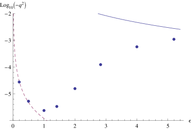
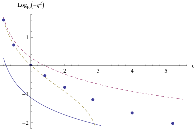
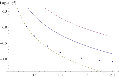
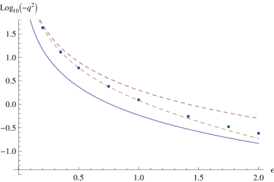
For the proof of these facts, see Appendix.B. Furthermore, we experientially find that, with several typical sets of parameters and ,
| (2.17) |
and interestingly
| (2.18) |
although we have no proof. We numerically solved this equation for several parameters as shown in Figure -719 and -718. The left and right panels in both figures correspond to and 2, respectively.
For later convenience, we introduce the “physical” mass for the unstable mode. The eigenvalue for the R-string with winding number is translated in terms of the mass for the canonically normalized messenger field as
| (2.19) |
We will use it later for the physical considerations. Here an non-trivial fact is observed.
3 R-string in thermal plasma
Now we turn to the stabilization of the R-strings. As shown in the previous section, R-strings in the (Minkowski background) vacuum are unstable and unavoidably deform to R-tubes. As discussed in [8], R-tubes are basically unstable objects and cause, in turn, the roll-over process to push the whole Universe into the unwanted SUSY vacuum with a finite time. Therefore, one may consider that the SUSY-breaking models with the spontaneous R-symmetry breaking are disfavored if the R-symmetry has once been restored in the cosmic history and R-strings have been formed.
However, the realistic Universe is neither described by the Minkowski space time nor in the vacuum. It contains several ingredients that can deform the potential for the R-string sector. It may be possible to stabilize the R-strings. The most effective contribution would be the thermal potential in the existence of the thermal plasma and hence we focus on the thermal effect in the following333The Hubble induced masses generated from the Planck suppressed interaction between the R-string sector and inflaton also exist during the inflaton oscillation dominated era before reheating. However, we can show easily that it cannot stabilize R-strings sufficiently in the wide range of parameter space. .
Here we should note that we do not have to stabilize R-strings up to the present time. As explained in [41], R-string networks, if they are stabilized, vanish when the Hubble parameter of the Universe becomes sufficiently small, [42]. This is because the constant term is added in the supergravity superpotential to compensate the vanishing cosmological constant, and such a constant term explicitly breaks the R-symmetry and makes the R-string healthily unstable. From the explicit R-symmetry breaking effect, the R-axion, which is the phase direction of the SUSY-breaking field acquires a mass. Thus, when the Hubble parameter decreases sufficiently, the R-string network turns to the R-string-domain wall system, which collapses to R-axion particles immediately [42]. Therefore, we only have to stabilize R-strings up to the Hubble time corresponding to .
We also note that high reheating temperature is not necessarily required in our discussion. In the gauge mediated SUSY-breaking, there is a severe constraint on the reheating temperature from the gravitino problem444For the cosmological constraint from R-axions, see [41].. Therefore, thermal plasma seems to be difficult to modify the potential for the R-string sector. However, even before reheating during the inflaton oscillation dominated era, thermal plasma of supersymmetric standard model particles does exist from the partial decay of inflaton quanta, of which temperature is larger than the reheating temperature. Thus, it is plausible to consider the thermal potential for the R-string sector that is generated by the thermal plasma. In this section, we demonstrate that the unstable modes shown in the previous section can be stabilized by the thermal effect assuming the existence of thermal plasma with sufficiently high temperature. We will revisit the cosmic history with R-strings in the next section.
3.1 Thermal potential for messenger
In this subsection, we study the thermal potential in the hidden sector generated by the supersymmetric standard model thermal plasma through the gauge interaction. Here we assume that the temperature of thermal plasma is relatively low, and the moduli field and messenger field are not thermalized555For smaller temperature, the number density of heavy fields is Boltzmann suppressed, if ever, and hence they cannot be in thermal equilibrium in the expanding Universe. The mass of messenger fields around the R-string core is typically small enough to be thermalized. However, the width of R-string is too small for the messenger fields to be thermalized and we do not consider the effect of messenger thermalization. since we are interested in the last stage when the stabilization mechanism is effective.
Since nonvanishing messenger field values generate the Standard model gauge boson (and gaugino) mass, their one-loop effective thermal potential generates thermal correction to the scalar potential for the messenger fields (see [43] for a review and references therein),
| (3.1) |
where factor comes from the degree of freedom of the massive vector bosons666Remember that for simplicity we consider only the singlet messenger fields and with the charges . It is straightforward to proceed the argument to the full theory. and
| (3.2) |
For smaller messenger field values, we can use the high temperature expansion,
| (3.3) |
with . Then, the messenger fields acquire the effective mass, , as
| (3.4) |
We can expect that the R-string is stabilized if the thermal mass is larger than the physical mass of the tachyonic mode discussed in the previous section. The ratio of the messenger mass to the tachyonic mode mass is given by
| (3.5) |
which is larger than one in a wide range of parameter space. Thus, even in a low temperature, , the thermal mass can be comparable to the physical tachyonic mode mass for the R-string, and hence it is enough to use the above thermal potential to study stability of tachyonic modes.
To complete the argument on thermal effects, we comment on the higher temperature situation, . In this case, the messenger fields are also thermalized and extra contribution to thermal effective potential to messenger direction is generated,
| (3.6) |
where
| (3.7) |
Here, the fermion contribution comes from the diagram with gaugino and messengino, whereas the additional scalar contribution comes from the messenger scalar loop, which acquires mass from the D-term. We should note that the thermal potential for is also generated by messenger fields, . However, if is small, the thermal potential can be much smaller than the zero-temperature mass of at . Thus, we can neglect thermal corrections to the potential for the field here.
Finally, we comment on the extension of the gauge theory. So far, we have considered the singlet messenger fields, and , with the charges for simplicity. It is straightforward to extend our discussions for generic messenger fields, and with the vector-like representations, , under the gauge symmetry. In such a generic case, all of the gauge bosons contribute to induce the thermal potential of the messenger fields. Such a thermal potential is obtained by replacing in (3.1) and (3.4) by
| (3.8) |
where and denote the quadratic Casimir indices of the representations of and , respectively, and denotes the hypercharge of . Thus, our discussions in the following sections can be extended into the full visible gauge theory by replacing .
3.2 Tachyonic mode around R-string
Now we are ready to study thermal effects on R-string. Firstly, let us see how the tachyonic mass of the R-string can be modified by the thermal effect in (3.1). To study this, we have only to pay attention to an infinitesimal fluctuation , which indicates that we can use the high temperature approximation,
| (3.9) |
The second term in the above gives a constant shift of the potential in (2.14) as
| (3.10) |
and resultantly a mass eigenvalue also accepts the constant shift,
| (3.11) |
It is straightforward to define the -th critical temperature, , where , that is,
| (3.12) |
and then we find the following properties
| (3.13) |
At a temperature larger than , the tachyonic mass changes to massive one and therefore the R-string with a winding number is stable.
As an illustration, we show the low energy effective potential for the light mode. As in [8], to uncover the existence of light unstable mode, which is almost frozen in the relaxation method, we vary the initial profile function. To be concrete, the following initial conditions with various values of are used for
| (3.14) | |||
Also, to represent the size of the tube, we define the following parameter,
| (3.15) |
We also introduce the dimensionless temperature as
| (3.16) |
where as is shown in (3.3), the parameter for the thermal potential is written as
| (3.17) |
To see how the stabilization mechanism works, we define the dimensionless energy as
| (3.18) |
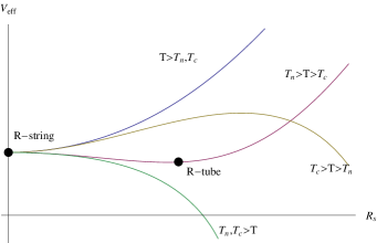
at the relaxation time (for quick introduction to the relaxation method, see appendix A in [8]). Here we removed a contribution of the vacuum energy density . denotes the cut-off of the energy and we set . Since we cannot follow the evolution of the system in the relaxation method to , we evaluate it at . In Figure -717, we plot and for various initial conditions for and . Here we take the parameters as , , and . For these parameters, we can expect the R-string is stabilized for . As one can see from the Figure, is the local energy minimum of the field configuration, which implies the R-string is stabilized for , whereas it does not seem to be local minimum for , as expected. Thus, we conclude that the R-strings are stabilized for . It is interesting that the R-strings are stabilized even if the thermal mass for the messenger field is smaller than its zero temperature mass at the origin, . Finally, it is worth emphasizing that in the Figure -717, we draw the effective potential until relatively larger value of just for reference where high temperature expansion is no longer valid. Thus, only the behavior in small region is reliable, which is enough to guarantee the stability of the R-string.


3.3 Uplifted SUSY vacuum and stable R-tube
We here point out that there is a phenomenologically safe situation even when the R-strings are unstable and they deform to R-tubes. One of the interesting features of thermal effects is lifting the lower energy vacuum. Since SUSY is broken by the thermal effect, the SUSY vacuum can be lifted and the SUSY-breaking vacuum becomes thermodynamically favored compared to the lower energy vacuum. To see that, let us focus on the messenger direction at and .
| (3.19) |
where and
| (3.20) |
Here, we subtracted because the SUSY breaking vacuum also gets lifted by thermal effect. It is given by constant term at . Thus, it is useful to subtract it and define the potential as above. Here we can show the following inequalities
| (3.21) |
The would-be SUSY vacuum is determined by
| (3.22) |
The critical temperature, , at which the would-be SUSY vacuum and SUSY breaking vacuum become the same energy density, is determined by the following equation777Note that the field configuration in the realistic expanding Universe does not follow perfectly the R-tube solution. However, at least the R-tube solution is stable, the dangerous roll-over process will not cause and hence this consideration gives a good condition to avoid the roll-over problem. ,
| (3.23) |
By taking derivatives with respect to and of the above equation, we find that is a monotonically increasing function of and as
| (3.24) |
where we used the inequalities (3.21).
For or , that is , the potential reduces to
| (3.25) |
and thus, the functions and are explicitly given as
| (3.26) |
Then, the inequality (2.18) means that, for sufficiently large ,
| (3.27) |
In the opposite limit, or , we also find the explicit form888In our model, the gauge group is completely broken in the SUSY-vacuum and hence thermal logarithmic potential [44] for low temperature regime would not arise. However, even if it appears, it also has an effect to lift up the SUSY-vacuum, and hence the basic feature does not change if it is positive. In the case of negative thermal logarithmic potential, the stabilization mechanism for R-tube does not work with or .
| (3.28) |
For , therefore, we find the inequality with an arbitrary .
Here, we show that the critical temperature of the R-string with the minimal winding number is always lower than . By using (3.22), (3.24) and (3.26), we fine the following relation
| (3.29) |
From the properties noted in the above we can draw a phase diagram as Figure -716. Note that an R-tube with the minimal winding number is always unstable.
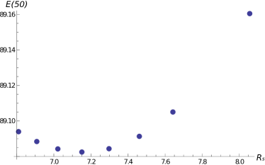
As an illustration, we show a stable R-tube solution with the winding number . We take parameters and , which allow us to use limit as (3.26) though it is not good enough. From the Figure -719, we see that the tachyonic mass is for and . Since , the R-string with is unstable and turns out to become the R-tube in that case. On the other hand, is enough to uplift the SUSY vacuum to stabilize the R-tube as . In the Figure -715 we show the low energy effective potential for the R-tube solution with , , . Clearly there exists the minimum around .
Finally, let us comment on the validity to use the thermal potential. In deriving the thermal potential, we assumed homogeneity at least of order . On the other hand, when we study the stability of solution we put the R-string/R-tube solution which generates inhomogenioety in the space. A condition of the validity to the thermal potential can be roughly estimated as
| (3.30) |
In the stabilized R-string solution, there is no space dependence of . Thus this condition is satisfied. However, as for the R-tube solution shown above, there is space dependence. Using the dimensionless temperature in (3.16), we can estimate the validity condition,
| (3.31) |
The numerical analysis on the R-tube solution for leads to . Thus, our numerical results are still under control for a proper value of .
4 Application to the expanding Universe
Now we study how the discussion in the previous section is applied to the constraints on the realistic cosmology with expanding Universe. Here we focus on the vacuum selection and the way to avoid the roll-over problem. There are also constraints from the cosmological gravitino or moduli problem, and R-axion particle abundances, but these are beyond the scope of the present paper. For the discussion on such problems, see [40] and [41].
Let us follow cosmic histories in our scenario schematically. The thermal mass for the messengers is given by , with being the numerical factor of the order of unity that counts the number of fields contributing the thermal mass. If messengers enter thermal plasma, it generates thermal mass to the field, as , where is the numerical factor of the order of unity. Note that during the inflaton oscillation dominated era, the temperature and the Hubble parameter are related by
| (4.1) |
where is the effective relativistic degrees of freedom and denotes the reheating temperature. There are also the so-called Hubble induced mass for and messengers, , which is generated from the Planck suppressed interaction between inflaton and these fields in supergravity. For small enough ,
| (4.2) |
the Hubble induced mass overwhelms the thermal mass for fields when , and in the following, we consider such a situation. Here, we assume the inflaton oscillation dominated era since the gravitino problem requires relatively small reheating temperature.
At a high temperature in the inflaton oscillation dominated era, the thermal masses or the Hubble induced mass for and messenger fields restore the symmetry and these fields are set at the origin. As the temperature and the Hubble parameter decreases, the Hubble induced mass or the thermal mass can no longer fix the fields at the origin and symmetries are spontaneously broken. If the Hubble induced mass for the becomes inefficient earlier than the thermal mass for messenger fields, the SUSY-breaking vacuum is naturally selected associated with the R-string formation. This condition can be written as
| (4.3) |
which is rewritten in terms of the constraint on the reheating temperature,
| (4.4) |
In the other case, if , the Hubble induced mass for always becomes inefficient before that for become inefficient as discussed in section 2.1. Therefore, one of the inequality (2.10) and the inequality (4.4) is needed to be satisfied for selecting the SUSY-breaking vacuum as showed in the Figure -714.
After acquires the nonvanishing field value, the R-strings are formed and our discussion in the previous section can be applied. We have shown that any R-strings with arbitrary winding numbers are stabilized for sufficiently high temperature,
| (4.5) |
However, practically, it may be sufficient to protect only the mode with . In this case, the condition for the stabilization can be written as
| (4.6) |
As shown in (3.29), is always higher than . Since the R-string networks turn to the R-string-domain wall networks and immediately decay to R-axion particles at [42], we can avoid the roll-over problem if the stabilization mechanism discussed above works at that time. As shown in the previous section, for , is satisfied. Thus, the above constraints can be rewritten as follows,
| (4.7) |
which is rewritten in terms of the constraint on the reheating temperature,
| (4.8) |
and
| (4.9) |
which, in turn, is expressed as the constraint on the reheating temperature,
| (4.10) |
Note that a quantity , which is compared with a value in Eq.(2.12), can take a value in the limit of and also in a case of , and thus there are both cases of and whereas inequalities are always satisfied.
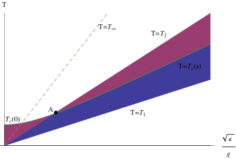
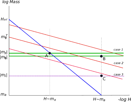
In Figure -713, we illustrate thermal histories by showing Hubble parameter dependences of various mass terms. In this figure we assumed just to draw this figure concretely. The blue line is the Hubble induced mass linear in . The red lines represent the thermal masses for the messengers with three different reheating temperatures. The horizontal green lines are the sizes of the tachyonic masses and at the origin with the following relation,
| (4.11) |
Note that depending on the two parameters, the order of the two masses is changed. Below we will show that the cases 1 and 2 in Figure -713 realize the successful vacuum selection. At the point A, the Hubble parameter becomes comparable to the size of tachyonic mass of at the origin, so the vacuum starts to slide down to the SUSY breaking vacuum. Sine the condition (4.3) is satisfied in these two cases, the SUSY breaking vacuum is successfully chosen. The points B and C represent the points where and are satisfied, respectively. In summary, the case 1 passes both the vacuum selection and stabilization of all R-strings with arbitrary winding number, whereas the case 2 passes the vacuum selection but stabilizes only the R-string with . The case 3 is ruled out by the vacuum selection if . With typical values of , the condition (4.8) is too strong to be satisfied, and the case 2 or the case 3 are preferred where a value of plays a quite important role.
As a reference, we compare these results to the constraint on the reheating temperature from the gravitino problem [45],
| (4.12) |
where denotes the gaugino mass. This condition comes from the constraint for the thermally produced gravitinos at the time of reheating not to overclose the Universe. Note that there may be late time entropy production from the moduli decay, which would relax the constraint on the reheating temperature, but this upper bound on the reheating temperature is a good reference value.
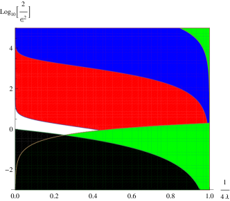
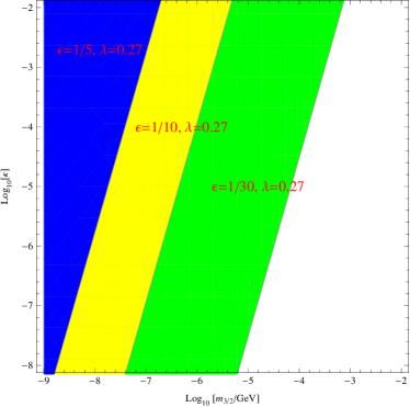
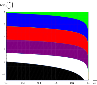
Figure -712 shows the window satisfying in the parameter space. We can see that there is a definite parameter space. For relatively large , a small gravitino mass is favored by the vacuum selection. Let us show the existence of non-zero window for . In Figure -711, we show regions satisfying . Here the coefficient is roughly estimated order one, . We adopt the gaugino mass in the gauge mediation as
| (4.13) |
where we assume a small hierarchy between gaugino mass and squark mass by introducing the small parameter coefficient which can be interpreted as the R-breaking effect for Majorana gaugino mass.
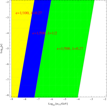
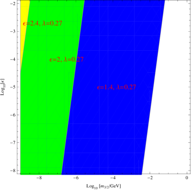
Finally we show examples for the case in Figure -710. Here we have used the numerical results for the tachyonic masses shown in Figure -719.
In conclusion, we surely have the scenarios that are free from the roll-over problem, avoiding the thermally produced gravitino problem. For this mechanism the value of a tachyonic mass of a fluctuation around the R-string configuration, , often plays a quite important role. This value is very sensitive with details of the model and can take a value with a quite wide range as we discussed, and thus, one has to always check this when building a more realistic model. Of course, there are also constraints from the moduli problem, the moduli induced gravitino problem, and R-axion problems, which are beyond the scope of the present study. We emphasize that our study is helpful for the future model building and studying the constraint on such models.
5 Discussion
In this paper, we focused on gauge mediation models and studied the thermal potential to the messenger generated by the thermal plasma of the standard model particles. However, in the gravity mediations, interactions to the standard model particles are suppressed by the Plank mass. It is not obvious to get large enough thermal potential to stabilize the unstable modes. However, in this case, there is one interesting possibility to stabilize unstable modes. Supergravity corrections also provide a positive mass term to the fields and ,
| (5.1) | |||||
| (5.2) | |||||
| (5.3) |
where is the F-term of and denote the constant term in the superpotential, we have not explicitly written similar terms for and we used the condition for the cancellation of the cosmological constant. From the last equality, we see that the mass is positive. In gravity mediation models, the SUSY breaking scale is relatively large. Therefore, if the gravitino mass satisfies the following inequality,
| (5.4) |
then it may be possible to stabilize R-strings with low winding number. As long as is very small, this condition is satisfied. Also, it is worth mentioning that in such a large SUSY breaking, the axion mass can be larger than the symmetry breaking scale, . In this case, explicit breaking effects are significant, so the R-string is immediately broken after its formation.
From our study, it may be plausible to assume that in a realistic gauge mediation model with spontaneous R-breaking, rolling over the potential hill by the unstable solitons does not occur. In this case, we have to impose further cosmological conditions, such as the moduli problem or the moduli induced gravitino problem studied in Ref. [40]. Moreover, as intensively studied in [41], when the R-string decay by axionic domain wall, it produces a large amount of R-axions. As for the long-lived R-axion, cosmological constraints such as Big Bang Nucleosynthesis and CMB observation severely constrain the parameter space [41].
Acknowledgement
The authors would like to thank W. Buchmüller, Y. Hamada, and T. Konstandin for useful comments and discussions. TK is supported in part by the Grant-in-Aid for the Global COE Program ”The Next Generation of Physics, Spun from Universality and Emergence” and the JSPS Grant-in-Aid for Scientific Research (A) No. 22244030 from the Ministry of Education, Culture,Sports, Science and Technology of Japan. YO’s research is supported by The Hakubi Center for Advanced Research, Kyoto University.
Appendix A Property of
Near the core of R-string, the solution behaves as
| (A.1) |
For large a property of a coefficient can be discussed as follows. Let us consider the following limit of the action after extracting the vacuum energy
| (A.2) |
with a redefinition of the function and the coordinate
| (A.3) |
In this limit, we also have a string solution with winding number and this solution behaves as
| (A.4) |
Note that is a constant and depends on only the number . We know that the radius of R-string is estimated as , and this fact implies that
| (A.5) |
Figure -709 shows the numerical result in the limit of (A.2), where is well approximated by . Therefore, we conclude that dependence of for large (and sufficiently large ) is given by
| (A.6) |

Appendix B Properties of the tachyonic mass
The first excited mode around the R-string has the point so that
| (B.1) |
This value of must represent a scale of this excitation mode and thus the following quantity should be of order one,
| (B.2) |
The above two equations give rough estimations of as follows. Let us assume that the following inequality
| (B.3) |
Under this assumption (B.1) can be solved as
| (B.4) |
Therefore we can use under the assumption and combining (B.2) we find
| (B.5) |
This result reads
| (B.6) |
The assumption (B.3) is satisfied if
| (B.7) |
Let us remember that a value of is proportional to for large and for large and can be expected to be although depends on and slightly. Sufficiently large , large and small satisfy the above and therefore in several limits we find
| (B.8) |
whereas the case with gives an important exception as
| (B.9) |
References
- [1] K. A. Intriligator, N. Seiberg and D. Shih, “Dynamical SUSY breaking in meta-stable vacua,” JHEP 0604, 021 (2006) [hep-th/0602239]; “Supersymmetry breaking, R-symmetry breaking and metastable vacua,” JHEP 0707, 017 (2007) [hep-th/0703281].
- [2] H. Ooguri and Y. Ookouchi, “Landscape of supersymmetry breaking vacua in geometrically realized gauge theories,” Nucl. Phys. B 755, 239 (2006): “Meta-Stable Supersymmetry Breaking Vacua on Intersecting Branes,” Phys. Lett. B 641, 323 (2006)
- [3] R. Kitano, H. Ooguri and Y. Ookouchi, “Direct Mediation of Meta-Stable Supersymmetry Breaking,” Phys. Rev. D 75, 045022 (2007) [hep-ph/0612139].
- [4] H. Abe, T. Kobayashi and Y. Omura, “R-symmetry, supersymmetry breaking and metastable vacua in global and local supersymmetric theories,” JHEP 0711, 044 (2007) [arXiv:0708.3148 [hep-th]].
- [5] K. A. Intriligator and N. Seiberg, “Lectures on Supersymmetry Breaking,” Class. Quant. Grav. 24, S741 (2007) [hep-ph/0702069].
- [6] R. Kitano, H. Ooguri and Y. Ookouchi, “Supersymmetry Breaking and Gauge Mediation,” Ann. Rev. Nucl. Part. Sci. 60, 491 (2010) [arXiv:1001.4535 [hep-th]].
- [7] M. Dine and J. D. Mason, “Supersymmetry and Its Dynamical Breaking,” Rept. Prog. Phys. 74, 056201 (2011) [arXiv:1012.2836 [hep-th]].
- [8] M. Eto, Y. Hamada, K. Kamada, T. Kobayashi, K. Ohashi and Y. Ookouchi, “Cosmic R-string, R-tube and Vacuum Instability,” arXiv:1211.7237 [hep-th].
- [9] P. J. Steinhardt, “Monopole And Vortex Dissociation And Decay Of The False Vacuum,” Nucl. Phys. B 190, 583 (1981); Phys. Rev. D 24, 842 (1981).
- [10] Y. Hosotani, “Impurities In The Early Universe,” Phys. Rev. D 27, 789 (1983).
- [11] U. A. Yajnik, “Phase Transition Induced By Cosmic Strings,” Phys. Rev. D 34, 1237 (1986).
- [12] R. Kitano, “Gravitational Gauge Mediation,” Phys. Lett. B 641, 203 (2006) [hep-ph/0607090].
- [13] M. Ibe and R. Kitano, “Sweet Spot Supersymmetry,” JHEP 0708, 016 (2007) [arXiv:0705.3686 [hep-ph]].
- [14] D. Shih, “Spontaneous R-symmetry breaking in O’Raifeartaigh models,” JHEP 0802, 091 (2008) [hep-th/0703196].
- [15] L. Ferretti, “R-symmetry breaking, rnuaway directions and global symmetries in O’Raifeartaigh models,” JHEP 0712, 064 (2007) [arXiv:0705.1959 [hep-th]].
- [16] H. Y. Cho and J. -C. Park, “Dynamical U(1)(R) breaking in the metastable vacua,” JHEP 0709, 122 (2007) [arXiv:0707.0716 [hep-ph]].
- [17] S. Abel, C. Durnford, J. Jaeckel and V. V. Khoze, “Dynamical breaking of U(1)(R) and supersymmetry in a metastable vacuum,” Phys. Lett. B 661, 201 (2008) [arXiv:0707.2958 [hep-ph]].
- [18] L. G. Aldrovandi and D. Marques, “Supersymmetry and R-symmetry breaking in models with non-canonical Kahler potential,” JHEP 0805, 022 (2008) [arXiv:0803.4163 [hep-th]].
- [19] L. M. Carpenter, M. Dine, G. Festuccia and J. D. Mason, “Implementing General Gauge Mediation,” Phys. Rev. D 79, 035002 (2009) [arXiv:0805.2944 [hep-ph]].
- [20] A. Giveon, A. Katz, Z. Komargodski and D. Shih, “Dynamical SUSY and R-symmetry breaking in SQCD with massive and massless flavors,” JHEP 0810, 092 (2008) [arXiv:0808.2901 [hep-th]].
- [21] Z. Sun, “Tree level spontaneous R-symmetry breaking in O’Raifeartaigh JHEP 0901, 002 (2009) [arXiv:0810.0477 [hep-th]].
- [22] T. Azeyanagi, T. Kobayashi, A. Ogasahara and K. Yoshioka, “Runaway, D term and R-symmetry Breaking,” Phys. Rev. D 86, 095026 (2012) [arXiv:1208.0796 [hep-ph]].
- [23] J. L. Evans, M. Ibe, M. Sudano and T. T. Yanagida, “Simplified R-Symmetry Breaking and Low-Scale Gauge Mediation,” JHEP 1203, 004 (2012) [arXiv:1103.4549 [hep-ph]].
- [24] J. Goodman, M. Ibe, Y. Shirman and F. Yu, “R-symmetry Matching In SUSY Breaking Models,” Phys. Rev. D 84, 045015 (2011) [arXiv:1106.1168 [hep-th]].
- [25] A. Amariti and D. Stone, “Spontaneous R-symmetry breaking from the renormalization group flow,” arXiv:1210.3028 [hep-th].
- [26] Z. Komargodski and D. Shih, “Notes on SUSY and R-Symmetry Breaking in Wess-Zumino Models,” JHEP 0904, 093 (2009) [arXiv:0902.0030 [hep-th]].
- [27] Y. Ookouchi, “Light Gaugino Problem in Direct Gauge Mediation,” Int. J. Mod. Phys. A 26, 4153 (2011) [arXiv:1107.2622 [hep-th]].
- [28] T. W. B. Kibble, “Some Implications of a Cosmological Phase Transition,” Phys. Rept. 67, 183 (1980); “Topology of Cosmic Domains and Strings,” J. Phys. A 9, 1387 (1976).
- [29] W. H. Zurek, “Cosmological experiments in superfluid helium?,” Nature 317, 505-508 (1985); “Cosmological experiments in condensed matter systems,” Phys. Rep. 276, 177-221 (1996).
- [30] M. Eto, K. Hashimoto and S. Terashima, “Solitons in Supersymmetry Breaking Meta-Stable Vacua,” JHEP 0703, 061 (2007) [hep-th/0610042].
- [31] K. Hanaki, M. Ibe, Y. Ookouchi and C. S. Park, “Constraints on Direct Gauge Mediation Models with Complex Representations,” JHEP 1108, 044 (2011) [arXiv:1106.0551 [hep-ph]].
- [32] J. Barnard, “Solitonic supersymmetry restoration,” JHEP 1101, 101 (2011) [arXiv:1011.4944 [hep-ph]]; “Condensate cosmology in O’Raifeartaigh models,” JHEP 1108, 058 (2011) [arXiv:1106.1182 [hep-ph]].
- [33] B. Kumar and U. A. Yajnik, “On stability of false vacuum in supersymmetric theories with cosmic strings,” Phys. Rev. D 79, 065001 (2009) [arXiv:0807.3254 [hep-th]]; “Graceful exit via monopoles in a theory with O’Raifeartaigh type supersymmetry breaking,” Nucl. Phys. B 831, 162 (2010) [arXiv:0908.3949 [hep-th]].
- [34] S. A. Abel, C. -S. Chu, J. Jaeckel and V. V. Khoze, “SUSY breaking by a metastable ground state: Why the early universe preferred the non-supersymmetric vacuum,” JHEP 0701, 089 (2007) [hep-th/0610334].
- [35] W. Fischler, V. Kaplunovsky, C. Krishnan, L. Mannelli and M. A. C. Torres, “Meta-Stable Supersymmetry Breaking in a Cooling Universe,” JHEP 0703, 107 (2007) [hep-th/0611018].
- [36] I. Dalianis and Z. Lalak, “Cosmological vacuum selection and metastable susy breaking,” JHEP 1012, 045 (2010) [arXiv:1001.4106 [hep-ph]].
- [37] A. Katz, “On the Thermal History of Calculable Gauge Mediation,” JHEP 0910, 054 (2009) [arXiv:0907.3930 [hep-th]].
- [38] M. Arai, Y. Kobayashi and S. Sasaki, “R-symmetry Breaking and O’Raifeartaigh Model with Global Symmetries at Finite Temperature,” Phys. Rev. D 84, 125036 (2011) [arXiv:1103.4716 [hep-th]].
- [39] Y. Nakai and Y. Ookouchi, “Comments on Gaugino Mass and Landscape of Vacua,” JHEP 1101, 093 (2011) [arXiv:1010.5540 [hep-th]].
- [40] H. Fukushima, R. Kitano and F. Takahashi, “Cosmologically viable gauge mediation,” arXiv:1209.1531 [hep-ph].
- [41] Y. Hamada, K. Kamada, T. Kobayashi and Y. Ookouchi, “Cosmological constraints on spontaneous R-symmetry breaking models,” arXiv:1211.5662 [hep-ph].
- [42] P. Sikivie, “Of Axions, Domain Walls and the Early Universe,” Phys. Rev. Lett. 48, 1156 (1982); D. H. Lyth, “Estimates of the cosmological axion density,” Phys. Lett. B 275, 279 (1992); M. Nagasawa and M. Kawasaki, “Collapse of axionic domain wall and axion emission,” Phys. Rev. D 50, 4821 (1994) [astro-ph/9402066]; S. Chang, C. Hagmann and P. Sikivie, “Studies of the motion and decay of axion walls bounded by strings,” Phys. Rev. D 59, 023505 (1999) [hep-ph/9807374]; T. Hiramatsu, M. Kawasaki, K. ’i. Saikawa and T. Sekiguchi, “Production of dark matter axions from collapse of string-wall systems,” Phys. Rev. D 85, 105020 (2012) [Erratum-ibid. D 86, 089902 (2012)] [arXiv:1202.5851 [hep-ph]].
- [43] M. Quiros, “Finite temperature field theory and phase transitions,” hep-ph/9901312.
- [44] A. Anisimov and M. Dine, “Some issues in flat direction baryogenesis,” Nucl. Phys. B 619, 729 (2001) [hep-ph/0008058].
- [45] M. Kawasaki, K. Kohri and T. Moroi, “Hadronic decay of late - decaying particles and Big-Bang Nucleosynthesis,” Phys. Lett. B 625, 7 (2005) [astro-ph/0402490]; “Big-Bang nucleosynthesis and hadronic decay of long-lived massive particles,” Phys. Rev. D 71, 083502 (2005) [astro-ph/0408426].