Quasars Probing Quasars IV: Joint Constraints on the Circumgalactic Medium from Absorption and Emission

Abstract

We have constructed a sample of 29 close projected quasar pairs where the background quasar spectrum reveals absorption from optically thick H I gas associated with the foreground quasar. These unique sightlines allow us to study the quasar circumgalactic medium (CGM) in absorption and emission simultaneously, because the background quasar pinpoints large concentrations of gas where ${\rm Ly\alpha}$ emission, resulting from quasar-powered fluorescence, resonant ${\rm Ly\alpha}$ scattering, and/or cooling radiation, is expected. A sensitive search ($1\sigma$ surface-brightness limits of ${\rm SB}_{\rm{\rm Ly}\alpha}\simeq 3{\;\times\;10^{-18}}\,{\rm\,erg\,s^{-1}\,cm^{-2}\,arcsec^{-2}}$) for diffuse ${\rm Ly\alpha}$ emission in the environments of the foreground (predominantly radio-quiet) quasars is conducted using Gemini/GMOS and Keck/LRIS slit spectroscopy. We fail to detect large-scale $\sim 100\,{\rm\ kpc}$ ${\rm Ly\alpha}$ emission, neither at the location of the optically thick absorbers nor in the foreground quasar halos, in all cases except a single system. We interpret these non-detections as evidence that the gas detected in absorption is shadowed from the quasar UV radiation due to obscuration effects, which are frequently invoked in unified models of AGN. Small-scale $R_{\perp}\lesssim 50\,{\rm\ kpc}$ extended ${\rm Ly\alpha}$ nebulosities are detected in $34\%$ of our sample, which are likely the high-redshift analogs of the extended emission-line regions (EELRs) commonly observed around low-redshift ($z<0.5$) quasars. This may be fluorescent recombination radiation from a population of very dense clouds with a low covering fraction illuminated by the quasar. We also detect a compact high rest-frame equivalent width ($W_{{\rm Ly}\alpha}>50$Å) ${\rm Ly\alpha}$-emitter with luminosity $L_{{\rm Ly}\alpha}=2.1\pm 0.32{\;\times\;10^{41}}{\rm\,erg\,s^{-1}}$ at small impact parameter $R_{\perp}=134\,{\rm\ kpc}$ from one foreground quasar, and argue that it is more likely to result from quasar-powered fluorescence, than simply be a star-forming galaxy clustered around the quasar. Our observations imply that much deeper integrations with upcoming integral-field spectrometers such as MUSE and KCWI will be able to routinely detect a diffuse ${\rm Ly\alpha}$ glow around bright quasars on scales $R\sim 100\,{\rm\ kpc}$ and thus directly image the CGM.

1. Introduction

The ionizing radiation emitted by a luminous quasar can, like a flashlight, illuminate hydrogen in its vicinity, teaching us about the physical properties of gas in its surroundings. This is because photoionized hydrogen ultimately produces Ly$\alpha$ recombination photons, which are likely to escape the system. Whether this ‘fluorescent’ emission arises from the highly ionized Ly$\alpha$ forest clouds in the intergalactic medium (IGM) which are optically thin to ionizing photons, from the optically thick Lyman Limit Systems (LLSs) and damped Lyman-$\alpha$ systems (DLAs) detected as the strongest absorption lines in quasar spectra, or from the interstellar or circumgalactic medium (CGM) of the quasar host itself, the underlying principle is nevertheless the same – a fraction of the energy in the quasars’ UV continuum is ‘focused’ into line radiation and re-emitted back into space, informing us about the physical conditions of the emitting gas.

The idea of searching for fluorescent ${\rm Ly\alpha}$ emission from the intergalactic medium is not new. Hogan & Weymann (1987) first proposed that fluorescent emission might be detectable from the optically thin $N_{\rm HI}\lesssim 17.2$, Ly$\alpha$ forest clouds, which emit recombination photons because they are illuminated by the ambient extragalactic UV background. Gould & Weinberg (1996) made the crucial point that emission from the $N_{\rm HI}\gtrsim 17.2$ LSSs should be much brighter, because these clouds, being optically thick to Lyman continuum photons, absorb all the ionizing radiation incident upon them. Some $\sim 60\%$ of these ionizing photons result in ${\rm Ly\alpha}$ recombinations, and are ‘mirrored’ back as Ly$\alpha$ photons. Thus at the very faintest flux levels, UV background radiation should power a ubiquitous fluorescence signal, whereby all of the optically thick gas in the cosmic web would ‘glow’ in the ${\rm Ly\alpha}$ line (Hogan & Weymann 1987; Binette et al. 1993; Gould & Weinberg 1996; Cantalupo et al. 2005; Kollmeier et al. 2008).

Observationally, a number of increasingly sensitive searches for fluorescent radiation powered by the ambient UV background have been performed (Lowenthal et al. 1990; Bunker et al. 1998, 1999; Marleau et al. 1999), the deepest being the $\sim 100$ hour integration by Rauch et al. (2008) using the Very Large Telescope (VLT). Notwithstanding these efforts, the fluorescence signal has yet to be detected, and given independent estimates for the UV background intensity (Meiksin & White 2004; Bolton et al. 2005; Faucher-Giguère et al. 2008), the expected surface brightness ${\rm SB}_{{\rm Ly}\alpha}\simeq 1{\;\times\;10^{-20}}\,{\rm\,erg\,s^{-1}\,cm^{-2}\,arcsec^{-2}}$ is probably out of reach of current instrumentation. But in the regions proximate to a quasar the ionizing flux and resulting fluorescent surface brightness can be significantly enhanced, provided the quasar does not photoevaporate the nearby optically thick clouds. Fluorescence in the vicinity of a quasar has been searched for by a number of authors (Fynbo et al. 1999; Francis & Bland-Hawthorn 2004; Francis & McDonnell 2006; Adelberger et al. 2006; Cantalupo et al. 2007; Rauch et al. 2008) yielding either null or questionable detections. Perhaps most contentious is Adelberger et al. (2006), who purport to detect fluorescent emission from a DLA serendipitously detected in a background quasar spectrum which is $49^{\prime\prime}$ away from a luminous foreground quasar at $z=2.84$. Owing to the proximity of the foreground quasar, the ionizing flux should be enhanced by a factor of $\sim 5700$ over the UVB. However, the large continuum luminosity of this source and its implied relatively modest rest-frame ${\rm Ly\alpha}$ equivalent width (EW) of 75Å suggest that it may simply be ${\rm Ly\alpha}$ emission from the galaxy counterpart to the DLA, rather than quasar powered fluorescence.

Most recently, Cantalupo et al. (2012) performed a deep survey for ${\rm Ly\alpha}$ emission around a very bright $z=2.4$ quasar. In their narrow-band imaging, they report the detection of $\approx 100$ sources in their $3.5\,{\rm Mpc}\times 3.5\,{\rm Mpc}$ field of view, corresponding to a $\approx 5500$ comoving Mpc³ volume. They further note that a significant subset ($\approx 20\%$) exhibit ${\rm Ly\alpha}$ EWs far in excess of the maximum predicted value from star-forming regions (i.e. $W_{\rm Ly\alpha}>240$Å). These sources are the most convincing candidates to date for fluorescing gas in the extended environment (several Mpc separation) of, and powered by, a quasar. However it still remains unclear whether these candidate fluorescent emitters are counterparts to typical optically thick absorbers (LLSs and DLAs), and why more bright fluorescent emitters were not detected very close ($\lesssim 300\,{\rm kpc}$ proper) to the quasar. We will address both of these questions in this paper.

Besides illuminating nearby clouds in the IGM, a quasar may irradiate gas in its own host galaxy or circumgalactic halo. Rees (1988) suggested that cold CGM gas in the quasar host illuminated by the quasar could be detectable as an extended “fuzz” of fluorescent Ly$\alpha$ emission (see also Alam & Miralda-Escudé 2002; Haiman & Rees 2001). A number of groups have reported the detection of extended ${\rm Ly\alpha}$ emission in the vicinity of $z\sim 2-4$ quasars (Djorgovski et al. 1985; Hu & Cowie 1987; Heckman et al. 1991b, a; Bremer et al. 1992; Lehnert & Becker 1998; Bunker et al. 2003; Weidinger et al. 2004; Francis & Bland-Hawthorn 2004; Weidinger et al. 2005; Francis & McDonnell 2006; Christensen et al. 2006; Courbin et al. 2008; Hennawi et al. 2009; North et al. 2012). These efforts, some targeted and some serendipitous, reveal a diversity both in emission level, detection frequency, and physical extent, but detailed quantitative interpretation is hampered by differing methodologies (deep longslit spectroscopy versus narrow-band imaging), sample inhomogeneities (radio-loud versus radio-quiet), a broad range of redshifts (significant given $(1+z)^{4}$ surface brightness dimming and strong evolution in the quasar population), and ambiguities in detection criteria and definitions of the depth of the observations. Nevertheless, the emerging picture is that roughly half of quasars from $z\sim 2-4$ exhibit extended emission on scales of $10-50\,{\rm\ kpc}$ down to observed frame surface brightness levels of ${\rm SB}_{\rm Ly\alpha}\sim{\rm few}\times 10^{-17}{\rm\,erg\,s^{-1}\,cm^{-2}\,arcsec^{-2}}$. There is suggestive evidence that radio-loud quasars have brighter emission and a higher detection frequency (Heckman et al. 1991b), although high detection frequencies have also been reported in samples which are mostly radio-quiet (Christensen et al. 2006; North et al. 2012). Finally, this ${\rm Ly\alpha}$ emission may be powered by the same mechanism powering the extended emission line regions (EELRs) detected around low redshift $z<0.5$ type-I (e.g. Stockton et al. 2006; Husemann et al. 2012) and type-II (Greene et al. 2011) quasars, traced by [O III] and Balmer lines.

The brightest cases of ${\rm Ly\alpha}$ nebulosities around quasars have an average surface brightness ${\rm SB}_{{\rm Ly}\alpha}\sim 10^{-16}{\rm\,erg\,s^{-1}\,cm^{-2}\,arcsec^{-2}}$ ($z=2$) over a diameter of $\sim 100\,{\rm\ kpc}$, corresponding to a total Ly$\alpha$ luminosity of $L_{\rm Ly\alpha}\sim 10^{44.5}~{}{\rm\,erg\,s^{-1}}$. These nebulae bear a striking resemblance to the extended ${\rm Ly\alpha}$ emission typically observed around high-redshift radio galaxies (HzRG; e.g. McCarthy et al. 1990; McCarthy 1993; van Ojik et al. 1996; Nesvadba et al. 2006; Binette et al. 2006; Reuland et al. 2007; Villar-Martín et al. 2007; Miley & De Breuck 2008) as well as the so-called ${\rm Ly\alpha}$ ‘blobs’ (LABs; e.g. Fynbo et al. 1999; Steidel et al. 2000; Francis et al. 2001; Palunas et al. 2004; Matsuda et al. 2004; Dey et al. 2005; Colbert et al. 2006; Nilsson et al. 2006; Smith & Jarvis 2007). The primary difference between the nebulae around quasars versus those around HzRGs or ${\rm Ly\alpha}$ blobs, is that a strong source of ionizing photons (e.g. the quasar) is directly identified, but not for the HzRGs or blobs. Obscuration and orientation effects, as are often invoked in unified models of AGN (see e.g. Antonucci 1993; Elvis 2000), could be responsible for this difference. Indeed, there is ample evidence for obscured AGN in HzRGs (e.g. Miley & De Breuck 2008), and evidence for obscured AGN have been uncovered in several of the LABs (Chapman et al. 2004; Basu-Zych & Scharf 2004; Dey et al. 2005; Geach et al. 2007; Barrio et al. 2008; Smith et al. 2008), although there are several notable exceptions (Smith & Jarvis 2007; Nilsson et al. 2006; Ouchi et al. 2009).

Although photoionization by an AGN is perhaps the most plausible mechanism powering extended ${\rm Ly\alpha}$ nebulae, particularly when the quasar is directly observed, a litany of other mechanisms have also been put forward. Other sources of ionizing photons, such as fast radiative shocks powered by radio-jets (McCarthy et al. 1990; Heckman et al. 1991b, a) or starburst driven superwinds (Francis et al. 2001; Taniguchi & Shioya 2000; Taniguchi et al. 2001) have been discussed. It also been suggested that X-rays produced via inverse Compton scattering of CMB photons (and/or local far-IR photons) by relativistic electrons in radio jets (Scharf et al. 2003; Smail et al. 2009), could be the source of ionization. The possibility that extended ${\rm Ly\alpha}$ emission is powered by star-formation, either via stellar ionizing photons escaping from galaxies (Rauch et al. 2011), spatially extended star-formation (Ouchi et al. 2009; Rauch et al. 2012), or by pure scattering of ${\rm Ly\alpha}$ photons (Dijkstra et al. 2006a, c; Barnes & Haehnelt 2009, 2010; Barnes et al. 2011; Zheng et al. 2011; Steidel et al. 2011; Dijkstra & Kramer 2012), has also been considered. In addition to photoionization and scattering, a large body of theoretical work has suggested that ${\rm Ly\alpha}$ emission nebulae could result from ${\rm Ly\alpha}$ cooling radiation powered by gravitational collapse (Haiman et al. 2000; Fardal et al. 2001; Furlanetto et al. 2005; Yang et al. 2006; Dijkstra et al. 2006b; Dijkstra & Loeb 2009; Goerdt et al. 2010; Dayal et al. 2010; Bertone & Schaye 2010; Faucher-Giguère et al. 2010; Frank et al. 2012; Rosdahl & Blaizot 2012). This scenario is particularly fashionable in light of a plethora of work on the so-called ‘cold mode’ of cosmological accretion (Fardal et al. 2001; Katz et al. 2003; Kereš et al. 2005, 2009; Dekel & Birnboim 2006; Birnboim et al. 2007; Ocvirk et al. 2008; Brooks et al. 2009; Dekel et al. 2009), whereby a significant fraction of the gas accreting onto galaxies from the IGM remains cold $T\sim 10^{4}\,{\rm K}$, and funnels in along large-scale filaments. In the absence of significant metal-enrichment, collisionally excited Ly$\alpha$ is the primary coolant of $T\sim 10^{4}\,{\rm K}$ gas; hence the accreting gas could steadily radiate gravitational potential energy in the ${\rm Ly\alpha}$ line as it falls into the halo. While many studies have suggested that gravitational cooling radiation could power the LABs (Fardal et al. 2001; Furlanetto et al. 2005; Dijkstra & Loeb 2009; Goerdt et al. 2010; Faucher-Giguère et al. 2010; Rosdahl & Blaizot 2012; Frank et al. 2012), the predictions of these simulations are uncertain by orders of magnitude (e.g. Furlanetto et al. 2005; Faucher-Giguère et al. 2010; Rosdahl & Blaizot 2012; Hennawi & Prochaska 2013) because the emissivity of collisionally excited ${\rm Ly\alpha}$ is exponentially sensitive to gas temperature. Accurate prediction of the temperature requires solving a coupled radiative transfer and hydrodynamics problem which is not currently computational feasible (but see Rosdahl & Blaizot 2012).

Thus despite significant observational and theoretical efforts, the relationship between ${\rm Ly\alpha}$ nebulae in quasars, HzRGs, and LABs is rather confusing, and the physical process powering extended ${\rm Ly\alpha}$ emission remains an important unsolved problem. Questions also remain about ${\rm Ly\alpha}$ emission outside of quasar halos, on the larger scales relevant to quasar powered IGM fluorescence.

In this fourth paper of the ‘Quasars Probing Quasars’ series, we introduce a novel technique to tackle the important problem of emission from the CGM. We search for this emission from close projected quasar pairs, which have small angular separation on the sky but large line-of-sight separations such that the two quasars are physically unassociated. In these unique sightlines, absorption in the background (‘b/g’) quasar encodes information about the distribution of circumgalactic and intergalactic gas in the vicinity of the foreground (‘f/g’) quasar. This technique thus allows us to analyze the absorption-line and emission-line properties of gas around quasars simultaneously. We perform a systematic, spectroscopic survey for extended ${\rm Ly\alpha}$ emission in the vicinity ($R_{\perp}<600$ kpc) of $z\sim 2$ quasars, to typical $1\sigma$ surface-brightness limits of ${\rm SB}_{\rm{\rm Ly}\alpha}\simeq 3{\;\times\;10^{-18}}\,{\rm\,erg\,s^{-1}\,cm^{-2}\,arcsec^{-2}}$. The data are drawn from our survey of projected quasar pairs (Hennawi et al. 2006a), and we restrict our analysis to 29 projected pair systems for which the spectrum of the b/g quasar shows evidence for an LLS coincident with the redshift of the f/g quasar. If the f/g quasar is illuminating this optically thick gas, this is a prime candidate for bright ${\rm Ly\alpha}$ fluorescence and the the b/g quasar pinpoints the expected location of the emission. Independently, our observations provide a sensitive search for any extended ${\rm Ly\alpha}$ emission in the environment of $z\sim 2$ quasars, such as might be powered by ${\rm Ly\alpha}$ cooling radiation or any of the other physical mechanism just discussed. Our b/g quasar absorption-line measurements statistically map out the covering factor of optically thick absorption in the quasar CGM (Hennawi et al. 2006a; Hennawi & Prochaska 2007; Prochaska et al. 2012), and detailed absorption-line modeling places constraints on the physical properties of this gas (Prochaska & Hennawi 2009). Armed with this knowledge about the properties of the CGM, we can make direct predictions for the expected fluorescent emission and compare to our observations. Similarly, by combining our emission constraints from this study with the physical properties of the gas, we can directly constrain the heating rate of the CGM gas we detect in absorption, which is the subject of a companion paper (Hennawi & Prochaska 2013).

As we will frequently refer to other results from the ‘Quasars Probing Quasars’ (QPQ) series, we briefly review the basic approach and summarize the key results of each paper. In QPQ1 (Hennawi et al. 2006a) we introduced a novel technique to study the physical state of gas in the CGM of $z\simeq 2-3$ quasars, which are hosted by massive galaxies, using projected quasar pairs (see also Crotts 1989; Moller & Kjaergaard 1992; Bowen et al. 2006; Schulze et al. 2012; Farina et al. 2012). Spectroscopic observations of the b/g quasar in each pair reveals the nature of the IGM transverse to the f/g quasar on scales of a few 10 kpc to several Mpc. In QPQ1, we searched 149 b/g quasar spectra for optically thick absorption in the vicinity of $1.8<z_{\rm fg}<4.0$ luminous f/g quasars, and found a high-incidence of optically thick gas in the quasar hosts CGM. In QPQ2, we compared the statistics of this optically thick absorption in b/g sightlines to that observed along the line-of-sight, and argued that the f/g quasars emit their ionizing radiation anisotropcially or intermittently. An echelle spectrum of a projected quasar pair was presented in QPQ3 (Prochaska & Hennawi 2009), which resolved the velocity field and revealed the physical characteristics (metallicity, density, etc.) of the absorbing CGM gas. In QPQ5 (Prochaska et al. 2012), we used a significantly enlarged sample of projected quasar pair spectra to characterize the CGM of quasars with much improved statistics, focusing on the covering factor and EW distributions of H I and metal line absorbers.

This paper is organized as follows. In §2 we present a formalism which describes ${\rm Ly\alpha}$ emission powered by photoionization and scattering. In §3 we provide details of the quasar pair survey, our spectroscopic observations, and describe the selection of the quasar-absorber sample that was used to search for extended ${\rm Ly\alpha}$ emission. As we will show, a key quantity for interpreting the ${\rm Ly\alpha}$ emission properties of the f/g quasars is the covering factor of optically thick absorbers measured in background sightlines, which we also quantify in this section. A custom algorithm was developed to subtract off the quasar PSFs and search for faint diffuse extended emission which is described in §4. Our results are presented and discussed in §5, where we also compare to previous searches for ${\rm Ly\alpha}$ fluorescence. We summarize and conclude in §6. In Appendix A, we quantify the attenuation of ${\rm Ly\alpha}$ by dust grains for gas clouds with properties matching our absorbers, and conclude that dust extinction is not a significant effect. Throughout this paper we use a cosmological model with $\Omega_{m}=0.24$, $\Omega_{\Lambda}=0.76$, $h=0.70$ which is consistent with the most recent WMAP5 values (Komatsu et al. 2009). Unless otherwise specified, all distances are proper. It is helpful to remember that in the chosen cosmology, at redshift $z=2.0$, an angular separation of $\Delta\theta=1^{\prime\prime}$ corresponds to a proper transverse separation of $R_{\perp}=8.7\,{\rm\ kpc}$, and a velocity difference of $1500\,{\rm km~{}s}^{-1}$ corresponds to a radial redshift space distance of $s=7.7\,{\rm\ Mpc}$. A typical quasar at $z=2.0$ with an SDSS magnitude of $i=19$, has specific luminosity at the Lyman edge of $\log_{10}L_{\nu_{\rm LL}}\simeq 30.5$ (erg s^-1 Hz^-1), and at a distance of $R=100\,{\rm\ kpc}$ ($11.5^{\prime\prime}$ projected on the sky) the flux of ionizing photons would be a factor $g_{\rm UV}\simeq 3760$ times higher than the ambient extragalactic UV background. Finally, we use the terms optically thick absorbers and LLSs interchangeably, both referring to quasar absorption line systems with $\log N_{\rm HI}>17.2$, making them optically thick at the H I Lyman limit ($\tau_{\rm LL}\gtrsim 1$).

2. Formalism and Preliminaries

This section provides analytical estimates for the surface brightness of ${\rm Ly\alpha}$ emission from a variety of physical processes. We frame the discussion in terms of a circumgalactic medium filled with cool clouds, and we present results in terms of quantities which can be directly measured from absorption-line observations using background sightlines.

2.1. Cool Cloud Model

Bright emission in the ${\rm Ly\alpha}$ line typically occurs in gas at $T\sim 10^{4}\,{\rm K}$, thus we consider a highly idealized model of a population of cool gas clouds in quasar halos. Several studies have previously explored similar models (Mo & Miralda-Escude 1996; Maller & Bullock 2004), and others have focused specifically on extended ${\rm Ly\alpha}$ emission (Rees 1988; Haiman & Rees 2001; Haiman et al. 2000; Dijkstra & Loeb 2009). Nearly all of this work assumes the cool gas is in pressure equilibrium with a hot tenuous virialized plasma. Although there may be some evidence for pressure confinement from our our absorption-line measurements (Prochaska & Hennawi 2009), our conclusions about ${\rm Ly\alpha}$ emission do not depend on the existence of a hot phase.

We assume that the cool gas clouds observed in absorption are spherical with a single uniform hydrogen volume density $n_{\rm H}$, and that they are spatially uniformly distributed throughout a spherical halo of radius $R$. Although extremely simple, this model is also relevant, to within order unity geometric corrections, to more complicated distributions which vary with radius, or the filamentary structures expected in the cold accretion picture. In what follows, we often employ averages over the projected area of the spherical halo on the sky which we denote with angle brackets, e.g. the average line-of-sight distance through the halo is $\langle s\rangle=1/A\int sdA=4R/3$. Besides the volume density $n_{\rm H}$ and the size of the halo $R$, two other parameters completely specify the spatial distribution of the gas, namely the hydrogen column density of the individual clouds $N_{\rm H}$, and the cloud covering factor $f_{\rm C}$, which is similarly defined to be an average over the sphere. We focus on these four parameters ($R$ ,$n_{\rm H}$ ,$N_{\rm H}$ , $f_{\rm C}$) because they are either directly observable or are closely related to absorption-line observations.

All other quantities of interest can then be expressed in terms of these four parameters. For example, of particular interest for computing the ${\rm Ly\alpha}$ surface brightness is the volume filling factor defined as the ratio of the volume occupied by the clouds to the total volume, $f_{\rm V}=n_{\rm c}V_{\rm c}$, where $n_{\rm c}$ is the number density of clouds and $V_{\rm c}$ is their volume. The definition of the covering factor is

$$f_{\rm C}\equiv\langle\int\frac{df_{\rm C}}{ds}ds\rangle,$$ (1)

where $\frac{df_{\rm C}}{ds}=n_{\rm c}\sigma_{\rm c}$, and $\sigma_{\rm c}$ is the cloud cross-sectional area. This gives $f_{\rm C}=n_{\rm c}\sigma_{\rm c}4R/3$ for our case of uniformly distributed clouds. Note that in general the covering factor can be larger than unity. The corresponding volume filling factor can be written as

$$f_{\rm V}=\frac{3f_{\rm C}N_{\rm H}}{4Rn_{\rm H}},$$ (2)

and the total mass of cool gas is then

$$M_{\rm c}=\frac{4}{3}\pi R^{3}f_{\rm V}\frac{n_{\rm H}m_{\rm p}}{X}=\pi R^{2}f_{\rm C}N_{\rm H}\frac{m_{\rm p}}{X},$$ (3)

where $m_{\rm p}$ is the mass of the proton and $X=0.76$ is the hydrogen mass fraction.

As we will consider emission from objects at high redshift, for which the size of the emitting clouds could be unresolved by our instrument, the relevant observable is the surface brightness $({\rm\,erg\,s^{-1}\,cm^{-2}\,arcsec^{-2}})$ averaged over the projected area of a sphere as measured from Earth. The specific intensity of ${\rm Ly\alpha}$ from our spherical halo is given by integrating the equation of radiative transfer through the gas distribution

$$I_{{\rm Ly}\alpha}=\int j_{{\rm Ly}\alpha}ds,$$ (4)

where $j_{{\rm Ly}\alpha}$ is the volume emissivity per steradian $({\rm erg\,s^{-1}\,cm^{-3}\,ster^{-1}})$. In this and the following sections we will ignore the attenuation of ${\rm Ly\alpha}$ radiation caused by resonant scattering of gas within the halo itself or by the IGM, as well as extinction caused by dust. Scattering within the halo itself would only change the spatial distribution of the emission, and as we are averaging over apertures on the sky, this should produce small effects. We do however consider the resonant scattering of a point source of ${\rm Ly\alpha}$ photons from the quasar CGM in §2.3. Scattering by the IGM is likely negligible for the redshifts we consider (Zheng et al. 2011). We estimate the impact of extinction by dust in the Appendix, and demonstrate that it should not result in a significant reduction of the ${\rm Ly\alpha}$ emission.

We can then write the average surface brightness observed from Earth as

$${\rm SB}_{{\rm Ly}\alpha}\equiv\frac{1}{(1+z)^{4}}\langle I_{{\rm Ly}\alpha}\rangle=\frac{1}{(1+z)^{4}}\frac{1}{\pi R^{2}}\int j_{\rm{\rm Ly}\alpha}dV$$ (5)

where the factor of $(1+z)^{-4}$ accounts for cosmological surface brightness dimming. The corresponding total ${\rm Ly\alpha}$ luminosity is

$$L_{{\rm Ly}\alpha} = 4\pi^{2}(1+z)^{4}R^{2}{\rm SB}_{{\rm Ly}\alpha}$$

$$= 1.3{\;\times\;10^{44}}\left(\frac{1+z}{3.0}\right)^{4}\!\!\left(\frac{R}{100\,{\rm kpc}}\right)^{2}$$

$$\times \left(\frac{{\rm SB}_{{\rm Ly}\alpha}}{10^{-17}\,{\rm\,erg\,s^{-1}\,cm^{-2}\,arcsec^{-2}}}\right)\,{\rm erg\,s^{-1}}$$

2.2. ${\rm Ly\alpha}$ Fluorescence

For a low density gas, it is possible to separate contributions to the total ${\rm Ly\alpha}$ intensity into recombination and collisionally excited components (Chamberlain 1953). Observationally, extended ${\rm Ly\alpha}$ emission could have contributions from both mechanisms. Collisional excitation of neutral atoms and the subsequent emission of ${\rm Ly\alpha}$ can play an important role in the radiative cooling of $T\sim 10^{4}\,{\rm K}$ gas, and we explore this cooling radiation from the CGM of quasars in detail in a companion paper (Hennawi & Prochaska 2013). In what follows we consider recombination, which we will also refer to as ${\rm Ly\alpha}$ fluorescence, from a source of ionizing photons. A central point source with an $r^{-2}$ dependence is assumed, but our estimates can easily be generalized to other spatial distributions. We consider the two limiting cases where the gas clouds are either optically thin $N_{\rm HI}\ll 10^{17.2}\,{\rm cm}^{-2}$ or optically thick $N_{\rm HI}\gg 10^{17.2}\,{\rm cm}^{-2}$ to Lyman continuum photons. At intermediate neutral columns $\sim N_{\rm HI}\sim 10^{17.2}\,{\rm cm}^{-2}$ our simple approximations break down and more detailed radiative transfer calculations are necessary. In each case, we consider the limit where light from the quasar has otherwise been unattenuated by resonant scattering or dust.

2.2.1 Optically Thin

The recombination emissivity from the cool clouds is

$$j_{{\rm Ly}\alpha}=f_{\rm V}\frac{h\nu_{{\rm Ly}\alpha}}{4\pi}\eta_{\rm thin}n_{\rm e}n_{\rm p}\alpha_{\rm A}(T),$$ (7)

where $n_{\rm e}$ is the electron density, $n_{\rm p}$ is the proton density, $\eta_{\rm thin}=0.42$ is the fraction of recombinations which result in a ${\rm Ly\alpha}$ photon in the optically thin limit (Osterbrock & Ferland 2006; Gould & Weinberg 1996), and the factor of $f_{\rm V}$ accounts for the fact that the emitting clouds fill only a fraction of the volume. The case A recombination coefficient $\alpha_{\rm A}$ is a weak function of temperature $T$, and we evaluate it at $T=10,000\,{\rm K}$ where $\alpha_{A}=4.18{\;\times\;10^{-13}}\,{\rm cm^{-3}\,s^{-1}}$ (Osterbrock & Ferland 2006).

The electron and proton densities are determined by photoionization equilibrium,

$$n_{\rm HI}\Gamma=n_{\rm e}n_{\rm p}\alpha_{\rm A},$$ (8)

and the photoionization rate $\Gamma$ is given by

$$\Gamma=\frac{1}{4\pi r^{2}}\int_{\nu_{\rm LL}}^{\infty}\frac{L_{\nu}}{h\nu}\sigma_{\nu}d\nu.$$ (9)

Here $\nu_{\rm LL}$ is the frequency at the Lyman edge, and $\sigma_{\nu}$ is the hydrogen photoionization cross-section. We assume that the quasar’s spectral energy distribution obeys the power-law form $L_{\nu}=L_{\nu_{\rm LL}}(\nu/\nu_{\rm LL})^{-\alpha_{\rm Q}}$, blueward of $\nu_{\rm LL}$ and adopt a slope of $\alpha_{\rm Q}=1.57$ consistent with the measurements of Telfer et al. (2002). The quasar ionizing luminosity is then parameterized by $L_{\nu_{\rm LL}}$, the luminosity at the Lyman edge. Throughout this paper we estimate $L_{\nu_{\rm LL}}$ by tying the Telfer et al. (2002) power-law spectrum to the composite quasar spectrum of Vanden Berk et al. (2001), which can then be compared to the SDSS optical photometry covering rest-frame UV wavelengths (see Appendix A of QPQ1 for a detailed description of this procedure).

For all cases of interest to us, radiation fields are sufficiently intense that optically thin gas will always be highly-ionized. Under this assumption, the neutral fraction $x_{\rm HI}\equiv\frac{n_{\rm HI}}{n_{\rm H}}\ll 1$, hence $n_{\rm p}\approx n_{\rm H}$ and $n_{\rm e}\approx(1+Y/2X)n_{\rm H}$, where the helium and hydrogen mass fractions are $Y$ and $X$, respectively, and we have assumed all helium is doubly ionized.

Putting this all together, the observed ${\rm Ly\alpha}$ surface brightness is

$${\rm SB}_{{\rm Ly}\alpha} = \frac{\eta_{\rm thin}h\nu_{{\rm Ly}\alpha}}{4\pi(1+z)^{4}}\alpha_{\rm A}\left(1+\frac{Y}{2X}\right)n_{\rm H}f_{\rm C}N_{\rm H}$$

$$= 7.7\times 10^{-19}\left(\frac{1+z}{3.0}\right)^{-4}\!\!\left(\frac{f_{\rm C}}{1.0}\right)\left(\frac{n_{\rm H}}{0.1\,{\rm cm^{-3}}}\right)$$

$$\times \left(\frac{N_{\rm H}}{10^{20}\,{\rm cm^{-2}}}\right){\rm\,erg\,s^{-1}\,cm^{-2}\,arcsec^{-2}}$$

Note that photoionization equilibrium implies that $j_{{\rm Ly}\alpha}\propto\Gamma n_{\rm HI}$, but since the neutral fraction is inversely proportional to photoionization rate $x_{\rm HI}\approx\alpha_{\rm A}n_{\rm H}(1+Y/2X)/\Gamma$, the net effect is that ${\rm Ly\alpha}$ emission is independent of the luminosity of the ionizing source in the highly-ionized, optically-thin regime, provided that the ionizing source is bright enough to keep the gas highly ionized and optically thin. This fact can be exploited to obtain an expression for the neutral column density averaged over the area of the halo, $\langle N_{\rm HI}\rangle$, in terms of the observed surface brightness and ionizing luminosity:

$$\langle N_{\rm HI}\rangle = 2.2\times 10^{17}\left(\frac{1+z}{3.0}\right)^{-4}\!\!\left(\frac{L_{\nu_{\rm LL}}}{10^{30}\,{\rm erg\,s^{-1}\,Hz^{-1}}}\right)^{-1}$$

$$\times \left(\frac{R}{100\,{\rm kpc}}\right)^{2}\!\!\left(\frac{{\rm SB}_{{\rm Ly}\alpha}}{10^{-17}\,{\rm\,erg\,s^{-1}\,cm^{-2}\,arcsec^{-2}}}\right)\,{\rm cm^{-2}}.$$

In order for the optically thin approximation to be valid, the individual clouds must have $N_{\rm HI}\ll 10^{17.2}\,{\rm cm^{-2}}$. In optically thin photoionization equilibrium, the neutral fraction scales as $x_{\rm HI}\propto r^{2}$ so that the largest neutral columns will be attained at $R$, the edge of the halo. It thus follows that $\langle N_{\rm HI}\rangle<{\rm max}(N_{\rm HI})$ and hence if $\langle N_{\rm HI}\rangle>10^{17.2}\,{\rm cm}^{-2}$ then the clouds are definitely optically thick at some locations in the halo and the optically thin approximation breaks down. One can thus use eqn. (2.2.1) to compute $\langle N_{\rm HI}\rangle$ and directly test whether the optically thin approximation is valid, given only the observed ${\rm Ly\alpha}$ surface brightness and the size of the nebulae, provided that $L_{\nu_{\rm LL}}$ can be estimated, as in the case of ${\rm Ly\alpha}$ nebulae observed around quasars. If $\langle N_{\rm HI}\rangle>10^{17.2}\,{\rm cm}^{2}$ then the clouds cannot be optically thin. Note however that the converse is not true — both optically thin and optically thick clouds can result in $\langle N_{\rm HI}\rangle<10^{17.2}\,{\rm cm}^{-2}$ – a small value of $\langle N_{\rm HI}\rangle$ thus provides no definitive information about whether we are in the optically thin or thick regime.

2.2.2 Optically Thick

If the clouds are optically thick to ionizing radiation, they will no longer emit ${\rm Ly\alpha}$ proportional to the volume that they occupy because of self-shielding effects. Instead, a thin highly ionized skin will develop around each cloud, and nearly all recombinations and resulting ${\rm Ly\alpha}$ photons will originate in this skin. The cloud will then behave like a special ‘mirror’, converting a fraction $\eta_{\rm thick}=0.66$ of the ionizing photons it intercepts into ${\rm Ly\alpha}$ photons emitted at a uniform brightness (i.e the specific intensity leaving the surface is isotropic, see Gould & Weinberg 1996). Simulations including both ionizing radiative transfer and ${\rm Ly\alpha}$ resonant scattering (Cantalupo et al. 2005; Kollmeier et al. 2008) have shown, that for the case of a quasar illuminating an optically thick cloud, the true surface brightness is reduced from the ‘mirror’ value by a factor of $\simeq 2-4$. This reduction occurs because illumination and radiative transfer effects redistribute photons over a wide solid angle. We introduce a geometric reduction factor $f_{\rm gm}$ to account for this reduction. For the case of a transversely illuminated spherical ‘mirror’, the resulting ‘half-moon’ illumination pattern results in a $f_{\rm gm}=4/(3\pi)=0.42$ (Adelberger et al. 2006). We set $f_{\rm gm}=0.5$, which is consistent with the range seen in radiative transfer simulations (Cantalupo et al. 2005; Kollmeier et al. 2008). At a distance $R$ from a quasar, a mirror will emit a surface brightness

$${\rm SB}_{{\rm Ly}\alpha} = \frac{f_{\rm gm}\eta_{\rm thick}h\nu_{{\rm Ly}\alpha}}{(1+z)^{4}}\frac{\Phi}{\pi}$$

$$= 4.0\times 10^{-17}\left(\frac{1+z}{3.0}\right)^{-4}\!\!\left(\frac{f_{\rm gm}}{0.5}\right)\!\!\left(\frac{R}{100\,{\rm kpc}}\right)^{-2}$$

$$\times \left(\frac{L_{\nu_{\rm LL}}}{10^{30}\,{\rm erg\,s^{-1}\,Hz^{-1}}}\right){\rm\,erg\,s^{-1}\,cm^{-2}\,arcsec^{-2}}$$

where $\Phi$ $({\rm phot\,s^{-1}\,cm^{-2}})$ is the ionizing photon number flux

$$\Phi=\int_{\nu_{\rm LL}}^{\infty}\frac{F_{\nu}}{h\nu}d\nu=\frac{1}{4\pi r^{2}}\int_{\nu_{\rm LL}}^{\infty}\frac{L_{\nu}}{h\nu}d\nu.$$ (13)

The total observed flux from the mirror is simply proportional to the area of the mirror times this ${\rm SB}_{{\rm Ly}\alpha}$.

Now consider the case of a population of cool optically thick clouds, hence also mirrors, but which are spatially unresolved by our instrument. In this regime we can write the ${\rm Ly\alpha}$ volume emissivity as

$$j_{{\rm Ly}\alpha}=\frac{\eta_{\rm thick}h\nu_{{\rm Ly}\alpha}}{4\pi}n_{\rm c}\sigma_{\rm c}\Phi,$$ (14)

Note that there is no geometric reduction factor in this case. Conservation of photons requires that a fraction $\eta_{\rm thick}$ of the ionizing photons emerge as ${\rm Ly\alpha}$ photons, and the emissivity must be isotropic. Again integrating the equation of radiative transfer and averaging over area (eqns. 4 and 5), we obtain

$${\rm SB}_{{\rm Ly}\alpha} = \frac{\eta_{\rm thick}h\nu_{{\rm Ly}\alpha}}{4\pi(1+z)^{4}}f_{\rm C}\Phi(R/\sqrt{3})$$

$$= 6.0\times 10^{-17}\left(\frac{1+z}{3.0}\right)^{-4}\!\!\left(\frac{f_{\rm C}}{1.0}\right)\!\!\left(\frac{R}{100\,{\rm kpc}}\right)^{-2}$$

$$\times \left(\frac{L_{\nu_{\rm LL}}}{10^{30}\,{\rm erg\,s^{-1}\,Hz^{-1}}}\right){\rm\,erg\,s^{-1}\,cm^{-2}\,arcsec^{-2}}.$$

In the expression above it is understood that $f_{\rm C}$ is capped at $f_{\rm C}=1$, corresponding to the case where all ionizing photons are absorbed.

Thus in the optically thick limit, the emission depends only weakly on the amount of cool gas through the covering factor of the clouds, and scales linearly with the ionizing photon flux. This contrasts strongly with the highly ionized optically thin limit, where the surface brightness depends on the amount of cold gas through the combination $f_{\rm C}n_{\rm H}N_{\rm H}$, but not on the intensity of the ionizing source.

2.3. ${\rm Ly\alpha}$ Emission from Scattering

In this subsection we compute the surface brightness of extended ${\rm Ly\alpha}$ emission, produced via resonant scattering of a central source of ${\rm Ly\alpha}$ photons (i.e. the quasar) by the neutral gas in the CGM. By analogy with the optically thick fluorescence, the scattering surface brightness can be written as

$${\rm SB}_{{\rm Ly}\alpha}=\frac{h\nu_{{\rm Ly}\alpha}}{4\pi(1+z)^{4}}f_{\rm C}\Phi_{{\rm Ly}\alpha}(R/\sqrt{3})$$ (16)

where $f_{\rm C}$ now represents the covering factor of gas which is optically thick in the ${\rm Ly\alpha}$  transition (i.e. $N_{\rm HI}\gtrsim 10^{14}\,{\rm cm^{-2}}$). This will in general be much higher than the covering factor of clouds optically thick at the Lyman limit considered in §2.2.2. The quantity $\Phi_{{\rm Ly}\alpha}$ is the flux of ionizing photons emitted close enough to the ${\rm Ly\alpha}$ resonance to be scattered by gas in motion around the quasar

$$\Phi_{{\rm Ly}\alpha}\approx\frac{L_{\nu_{{\rm Ly}\alpha}}}{4\pi r^{2}h}\frac{\Delta\nu}{\nu_{{\rm Ly}\alpha}}=\frac{L_{\nu_{{\rm Ly}\alpha}}}{4\pi r^{2}h}\frac{W_{{\rm Ly}\alpha}}{\lambda_{{\rm Ly}\alpha}},$$ (17)

where we have introduced the rest-frame absorption equivalent width $W_{{\rm Ly}\alpha}$, and implicitly assumed that it is a very weak function of radius, as we demonstrate next.

The volume averaged neutral column density through our gas distribution is $\langle N_{\rm HI}\rangle=f_{\rm C}N_{\rm H}\langle x_{\rm HI}\rangle$, where $\langle x_{\rm HI}\rangle$ is the volume averaged neutral fraction determined from photoionization equilibrium (eqn. 8). These relations imply an average ${\rm Ly\alpha}$ optical depth

$$\langle\tau_{{\rm Ly}\alpha}\rangle = 253\left(\frac{N_{\rm H}}{10^{20}\,{\rm cm^{-2}}}\right)\!\left(\frac{n_{\rm H}}{0.1\,{\rm cm^{-3}}}\right)\!\left(\frac{b}{50\,{\rm km~{}s}^{-1}}\right)^{-1}$$ (18)

$$\times \left(\frac{f_{\rm C}}{1.0}\right)\!\!\left(\frac{R}{100\,{\rm kpc}}\right)^{2}\!\!\left(\frac{L_{\nu_{\rm LL}}}{10^{30}\,{\rm erg\,s^{-1}\,Hz^{-1}}}\right)^{-1}$$

where we have introduced the $b$-value describing turbulent and thermal motions of the absorbing gas. On the flat portion of the curve of growth $1\lesssim\tau_{{\rm Ly}\alpha}\lesssim 10^{4}$, the corresponding equivalent width is (see e.g. Draine 2011)

$$W_{{\rm Ly}\alpha}\approx 0.99\left(\frac{b}{50\,{\rm km~{}s}^{-1}}\right)\left(\frac{\sqrt{\ln\left(\langle\tau_{{\rm Ly}\alpha}\rangle/\ln 2\right)}}{2.1}\right){\rm\AA},$$ (19)

so that equivalent widths of $W_{{\rm Ly}\alpha}\simeq 1$Å are expected. We can finally write

$${\rm SB}_{{\rm Ly}\alpha} = 1.2\times 10^{-18}\left(\frac{1+z}{3.0}\right)^{-4}\!\!\left(\frac{f_{\rm C}}{1.0}\right)\!\!\left(\frac{R}{100\,{\rm kpc}}\right)^{-2}$$

$$\times \left(\frac{W_{{\rm Ly}\alpha}}{1.0\,{\rm\AA}}\right)\left(\frac{L_{\nu_{{\rm Ly}\alpha}}}{10^{31}\,{\rm erg\,s^{-1}\,Hz^{-1}}}\right)$$

$$\times {\rm\,erg\,s^{-1}\,cm^{-2}\,arcsec^{-2}},$$

where it is again understood that $f_{\rm C}<1$ in eqn. (2.3).

Because equivalent width is such a weak function of optical depth on the saturated part of the curve of growth (eqn. 19), $W_{{\rm Ly}\alpha}$ is approximately independent of the ionizing luminosity of the quasar as well as the details of the gas distribution. Thus the scattering surface brightness scales as ${\rm SB}_{{\rm Ly}\alpha}\propto f_{\rm C}\Phi_{{\rm Ly}\alpha}$, completely analogous to optically thick recombinations for which ${\rm SB}_{{\rm Ly}\alpha}\propto f_{\rm C}\Phi$ (eqn. 2.2.2). However, scattering will typically be about $\sim 100$ times fainter than optically thick recombinations if the covering factors are the same because $\eta_{\rm thick}\Phi/\Phi_{{\rm Ly}\alpha}\sim 100$, which results from the assumption of $W_{{\rm Ly}\alpha}\simeq 1.0\,{\rm\AA}$, and from the relative amount of ionizing photons to ${\rm Ly\alpha}$ photons emitted by a typical quasar. One expects this scattering emission to be important, therefore, only in regimes where the gas is optically thin at the Lyman limit. Indeed, the surface brightness of scattering (eqn. 2.3) and optically thin fluorescence (eqn. 2.2.1) can be comparable, but have very different dependencies on gas distribution and quasar luminosity. Throughout this work we estimate $L_{\nu_{{\rm Ly}\alpha}}$ by tying the composite quasar spectrum of (Vanden Berk et al. 2001) to the SDSS optical photometry (covering rest-frame UV wavelengths) and computing the peak of the ${\rm Ly\alpha}$ emission line.

2.4. An Illustrative Example

There are two important points that can be made about the surface brightness of extended ${\rm Ly\alpha}$ emission, and its implications for the supply of cool gas. First, optically thin and optically thick fluorescence can result in comparable levels of emission, as can pure resonant scattering of a central source of ${\rm Ly\alpha}$ photons. To complicate matters further, cooling radiation, that is collisional excitation of ${\rm Ly\alpha}$, can also lead to comparable emission. In general, the only way to determine which mechanism is at work is to use diagnostics from additional emission lines. For instance, the detection of strong extended Balmer line emission would be provide compelling evidence for recombinations, and effectively rule out scattering and cooling. But given that Balmer lines are redshifted into the near-IR for $z>2$, detecting even H$\alpha$ would be a daunting observational task because of the low expected surface brightness. Furthermore, even if one is certain that recombination is the physical mechanism, it is still typically impossible to ascertain the ionization state of the gas, and hence whether it is optically thin or thick.

The second and related point is that measurements of the ${\rm Ly\alpha}$ surface brightness alone cannot be used to determine the cool gas mass. For recombinations, the surface brightness scales as ${\rm SB}_{{\rm Ly}\alpha}\propto f_{\rm C}n_{\rm H}N_{\rm H}$ if the gas is optically thin (eqn. 2.2.1), or as ${\rm SB}_{{\rm Ly}\alpha}\propto\Phi f_{\rm C}$ if it is optically thick (eqn. 2.2.2). Whereas, for scattering the scaling is ${\rm SB}_{{\rm Ly}\alpha}\propto\Phi_{{\rm Ly}\alpha}f_{\rm C}$ (eqn. 2.3). The total cool gas mass scales with the different combination $M_{\rm c}\propto f_{\rm C}N_{\rm H}$ (eqn. 3). Even if we have perfect knowledge of the mechanism (recombinations versus scattering) and the ionization state (optically thin or optically thick), the cool gas mass is not uniquely specified by the ${\rm Ly\alpha}$ emission alone. Note that the situation is even worse for ${\rm Ly\alpha}$ cooling radiation because of an exponential dependence on an unknown gas temperature (Hennawi & Prochaska 2013). Thus even in the best-case scenario where Balmer line observations point to recombinations, one will not know whether the gas is optically thin or thick, and hence which dependence on physical parameters to use.

The following worked example illustrates the aforementioned issues. Consider a relatively bright $z=2$ quasar with apparent magnitude of $i=17.0$. Using the procedure in Appendix A of Hennawi et al. (2006a), we determine the specific luminosity to be, $\log_{10}L_{\nu_{\rm LL}}=31.3$ at the Lyman limit, and $\log_{10}L_{\nu_{{\rm Ly}\alpha}}=32.0$ in ${\rm Ly\alpha}$. Now consider three distinct cool gas distributions, one optically thin to ionizing photons with parameters ($R,n_{\rm H},N_{\rm H},f_{\rm C}$) = ($100\,{\rm kpc}$, $0.15\,{\rm cm^{-3}}$, $10^{21}\,{\rm cm^{-2}}$, 1.0), another optically thick to ionizing photons with ($R,n_{\rm H},N_{\rm H},f_{\rm C}$) = ($100\,{\rm kpc}$, $100\,{\rm cm^{-3}}$, $10^{20}\,{\rm cm^{-2}}$, 0.01), and a third optically thin to ionizing photons but optically thick to ${\rm Ly\alpha}$ photons with ($R,n_{\rm H},N_{\rm H},f_{\rm C}$) = ($100\,{\rm kpc}$, $30\,{\rm cm^{-3}}$, $10^{17}\,{\rm cm^{-2}}$, 2.0). These very different cool gas distributions result in nearly identical average ${\rm Ly\alpha}$ surface brightness ${\rm SB}_{{\rm Ly}\alpha}\approx 1.1-1.2{\;\times\;10^{-17}}\,{\rm\,erg\,s^{-1}\,cm^{-2}\,arcsec^{-2}}$ over an $R=100\,{\rm kpc}$ halo. For the first two models the emission is powered by photoionization, whereas for the third it is pure ${\rm Ly\alpha}$ scattering. But note also that for the first distribution, ${\rm Ly\alpha}$ scattering contributes at very nearly the same surface brightness level $\sim 1.1{\;\times\;10^{-17}}\,{\rm\,erg\,s^{-1}\,cm^{-2}\,arcsec^{-2}}$ as optically thin photoionization, implying that disentangling the two mechanisms via say detection of Balmer lines would be challenging. These sizes and surface brightness levels are in line with the brightest ${\rm Ly\alpha}$ blobs surveyed by Matsuda et al. (2004, 2011) (rescaled to $z=2$) as well as the extended ${\rm Ly\alpha}$ nebulae detected around $z\sim 2$ HzRGs (e.g. Villar-Martín et al. 2007) and radio-loud quasars (e.g. Heckman et al. 1991b). For the first optically thin model the total cool gas mass is $M_{\rm c}=3.3{\;\times\;10^{11}}{\rm\ M}_{\odot}$, for the second optically thick model it is $M_{\rm c}=2.5{\;\times\;10^{8}}{\rm\ M}_{\odot}$, and for the ${\rm Ly\alpha}$ scattering case it is $M_{\rm c}=6.6{\;\times\;10^{7}}{\rm\ M}_{\odot}$. Thus variations of $\sim 5000$ in the total gas mass can all lead to comparable levels of extended ${\rm Ly\alpha}$ emission, and even if one were sure that photoionization was powering the emission (from Balmer lines) and/or detected the source of ionizing photons (an unobscured quasar), there is no way to determine whether the gas is optically thin or thick. Plugging the observed observed surface brightness ${\rm SB}_{{\rm Ly}\alpha}$, distance $R$, and ionizing luminosity $L_{\nu_{\rm LL}}$ into eqn. (2.2.1) for the area averaged neutral column gives $\langle N_{\rm HI}\rangle=1.3{\;\times\;10^{16}}\,{\rm cm}^{-2}$, and thus we cannot distinguish an optically thin from an optically thick scenario.

2.5. Why Quasar Pairs?

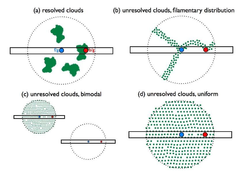
Figure 1.— Four scenarios for the spatial distribution of CGM gas in quasar halos which illustrate the usefulness of projected quasar pair observations. a) The absorbers/emitters are large resolved clouds at random locations in the quasar CGM. The background sightlines pinpoint the locations of optically thick clouds and thereby determine where to look for emission. For such large spatially resolved clouds, the relevant SB estimate is the mirror approximation (see eqn. 2.2.2). b) The clouds are small and hence spatially unresolved by our instrument, but gas resides in large resolved filamentary complexes which cover a fraction of the quasar halo. For longslit observations of quasar pairs, the b/g sightline intersects the filament by construction, again pinpointing where emission is expected. The average SBs that we computed in §2 underestimate the true SB of the filament, since they include a reduction by the covering factor $f_{\rm C}$, due to regions devoid of gas. c) The clouds are small and unresolved, but some quasars have cool gas complexes and others do not, and this bimodality in the gas supply is responsible for the variations that result in the observed covering factor. Quasar pairs are helpful because the background sightline identifies objects with large gas supply and hence where to search for emission. The average SBs that we computed in §2 are again underestimated because the covering factor includes objects with no gas. d) The clouds are small, unresolved, and distributed uniformly in the quasar halo. The background sightline does not provide useful information about where to search for emission. The average SB estimates in §2 appropriately account for the dilution by the covering factor $f_{\rm C}$, and this is the surface brightness that we expect to detect at any spatial position along the slit. For this case, a search for diffuse emission around isolated individual quasars, i.e. not residing in pairs, would be just as effective.

In the previous subsection we saw that a variety of physical processes and a wide range of gas distributions can all lead to comparable ${\rm Ly\alpha}$ emission. Hence, the great value of quasar pairs is that absorption-line observations of b/g quasars can provide crucial information about the physical properties of the gas in the CGM of the f/g quasar. Indeed, all the physical parameters ($R\,,n_{\rm H}\,,N_{\rm H}\,,f_{\rm C}$) can be determined from absorption line observations, provided that the covering factor is high enough for the clouds to be occasionally intercepted by b/g sightlines. For example, we map out the covering factor of optically thick absorption as a function of impact parameter (see Figure 2) in §3.4 (see also Hennawi et al. 2006a; Hennawi & Prochaska 2007; Prochaska et al. 2012), and find a high covering factor of cool, optically thick gas around all bright quasars at $z\sim 2$. In Prochaska & Hennawi (2009), we conducted detailed absorption line modeling of a single projected pair and determined that the column densities of the absorbing clouds are typically $N_{\rm H}\simeq 10^{20}\,{\rm cm}^{-2}$ and volume densities $n_{\rm H}\simeq 0.1-1\,{\rm cm}^{-3}$, although it is unclear whether this single system is representative. Armed with this knowledge of the gas distribution, one can then interpret the physical implications of the presence or absence of extended line emission.

Note however that the properties of gas with a very low covering factor $f_{\rm C}\sim 0.01$ are much more challenging to measure, since thousands of background sources would be required to map it out. Thus a crucial caveat in comparing absorption line observations to emission line observations is that the gas responsible for the detected emission may arise from clouds with a much lower covering factor than the gas dominating the absorption. Nevertheless, one can still make quantitative statements about the expected emission from the component of gas which is detected in absorption, which will have the highest covering factor. This is the approach adopted in this work.

But even if quasar pairs are useful for measuring the properties of the quasar CGM, why use quasar pairs, as opposed to individual isolated quasars, to searching for diffuse emission lines? Consider the following four scenarios which are illustrated schematically in Figure 1. a) The absorbers/emitters are large resolved clouds at a ‘random’ location in the quasar CGM (Figure 1a). In this case, the background sightlines pinpoint the locations of gas and thereby determine where to look for emission. This approach is akin to that taken by Adelberger et al. (2006), who purported to detect quasar fluorescence from an optically thick absorber detected in a b/g sightline. For this case of large resolved absorbers, the relevant SB estimate is the mirror approximation (see eqn. 2.2.2). b) Another possibility is that the clouds are small and hence unresolved by our instrument, but that the gas resides in large resolved filamentary complexes which cover a fraction of the quasar halo (Figure 1b). For this case, the b/g sightline intersects a filament by construction, and identifies the location where emission is expected via longslit observations of the quasar pair. Note that the average SBs computed in §2 would underestimate the true SB in this case, since they include a reduction by the covering factor $f_{\rm C}$, due to regions devoid of gas. c) It could also be that the clouds are small and hence unresolved, but some quasars have cool gas complexes and others do not. This bimodality in gas supply could result in the ‘hits’ and ’misses’ which give rise to the observed covering factor (Figure 1c). In this case, the quasar pairs are helpful since the background sightline identifies which objects to search for emission around, and the average SBs that we computed in §2 are again underestimated because the covering factor includes objects with no gas. d) Finally, the clouds could be small and hence unresolved, and distributed rather uniformly in the quasar halo (Figure 1d). In this case the background sightline does not provide us with useful information about where to search for emission. The average SB appropriately accounts for the dilution by the covering factor $f_{\rm C}$, and this is the SB that we expect to detect at any spatial position along the slit. For this case, a search for diffuse emission around isolated individual quasars, i.e. not residing in pairs, would be just as effective.

3. Quasar Pair Observations

Our goal is to conduct a sensitive search for extended ${\rm Ly\alpha}$ emission from the CGM and IGM around f/g quasars in quasar pairs, and to relate these emission constraints to our knowledge of the distribution of gas from absorption-line measurements of b/g sightlines. We concentrate on a unique sample of projected quasar pairs useful for exploring the CGM/IGM surrounding high-$z$ quasars and, by inference, the massive galaxies and dark matter halos which host them. We search for extended ${\rm Ly\alpha}$ emission around 29 $z\sim 2$ quasars, which are drawn from a parent sample of $68$ projected quasar pairs. Before delving into details, we briefly summarize the criteria used to select these 29 quasar pairs:

• the CGM/IGM around the f/g quasar exhibits strong and optically thick H I absorption in the b/g quasar sightline.

• the transverse separation of the pair and magnitude of the f/g quasar imply a fluorescent mirror surface brightness ${\rm SB}_{{\rm Ly}\alpha}>5{\;\times\;10^{-18}}{\rm\,erg\,s^{-1}\,cm^{-2}\,arcsec^{-2}}$ (see eqn. 2.2.2).

• a deep spectroscopic observation of the f/g quasar was obtained covering ${\rm Ly\alpha}$ , allowing us to perform a sensitive search for ${\rm Ly\alpha}$ emission on scales of tens to hundreds of kpc.

• the two quasars are separated by velocity $>2000\,{\rm km~{}s}^{-1}$, to ensure that they are indeed projected and not physically associated.

Although our search for extended ${\rm Ly\alpha}$ emission is focused on sightlines showing strong absorbers, we characterize the covering factor of optically thick absorbers using the full unbiased parent sample of 68 projected quasar pairs. This analysis demonstrates that the CGM surrounding $z\sim 2$ quasars has a high $>50\%$ covering fraction of optically thick gas to radius $R\approx 200$ kpc (see also Hennawi et al. 2006a; Hennawi & Prochaska 2007; Prochaska et al. 2012).

There are several reasons why we restrict our search for emission to only pair sightlines showing strong absorbers. First, in the context of fluorescence from the IGM, powered either by the UVB or boosted by a nearby quasar, emission from optically thick clouds will always dominate over optically thin gas because the density of gas in the optically thin ${\rm Ly\alpha}$ forest is just too low (e.g. Gould & Weinberg 1996, see also eqn. 2.2.1). Although this may not hold true in the CGM, where gas densities can be higher, note that the the mirror SB from a spatially resolved optically thick cloud is independent of the gas properties (eqn. 2.2.2), and the same holds for emission from a population of optically thick clouds provided the covering factor has been measured (eqn. 2.2.2). In contrast, optically thin emission depends on the combination $f_{\rm C}n_{\rm H}N_{\rm H}$ which is typically unknown. The upshot is that a non-detection of emission from gas which is optically thin could result either from $f_{\rm C}n_{\rm H}N_{\rm H}$ being too low, or because the gas is not illuminated by the quasar. Whereas, interpretation of non-detection of emission from optically thick gas is unambiguous, and implies that the gas is not illuminated by the quasar.

Note however, that given the high covering factor of optically thick gas in the quasar CGM, statistically, there is a high probability that any long-slit observation of a projected quasar pair will intersect optically thick material, even if the b/g sightline does not show absorption. We refer the reader to the discussion in §2.5 and Figure 1, which illustrates, nevertheless, why having a b/g sightline showing optically thick absorption can be advantageous.

In the following subsections we describe the details of the quasar pair survey, the spectroscopic observations, the definition of the quasar-absorber sample, and present our measurement of the covering factor of optically thick absorbers from the parent sample.

3.1. Quasar Pair Survey

Modern spectroscopic surveys select against close pairs of quasars because of fiber collisions. For the Sloan Digital Sky Survey (SDSS), the finite size of optical fibers precludes discovery of pairs with separation $<55^{\prime\prime}$ Thus, to find pairs with sub-arcminute separations, additional follow-up spectroscopy is required both to spectroscopically confirm quasar pair candidates, and to obtain spectra of sufficient quality to search for absorption line systems.

In an ongoing survey, close quasar pair candidates are selected from a photometric quasar catalog (Bovy et al. 2011, 2012), and are confirmed via spectroscopy on 4m class telescopes including: the 3.5m telescope at Apache Point Observatory (APO), the Mayall 4m telescope at Kitt Peak National Observatory (KPNO), the Multiple Mirror 6.5m Telescope, and the Calar Alto Observatory (CAHA) 3.5m telescope. Our continuing effort to discover quasar pairs is described in Hennawi (2004), Hennawi et al. (2006b), and Hennawi et al. (2010). To date about 350 pairs of quasars have been uncovered with impact parameter $R_{\perp}<300~{}{\rm kpc}$ and $z_{\rm fg}>1.6$. Projected pair sightlines were then observed with Keck and Gemini to obtain ‘science quality’ high signal-to-noise ratio (S/N) moderate resolution spectra. A subset of higher resolution spectra at echellette and echelle resolution have also been obtained, but these are not used in this work. This observational program has several science goals: measure the small-scale quasar clustering of quasars (Hennawi et al. 2006b; Myers et al. 2008; Hennawi et al. 2010; Shen et al. 2009), to measure small scale transverse Ly$\alpha$ forest correlations (Rorai et al. in prep), to characterize the transverse proximity effect (Hennawi et al., in prep.), and to use the b/g sightline to characterize the circumgalactic medium of the f/g quasar (Hennawi et al. 2006a; Hennawi & Prochaska 2007; Prochaska & Hennawi 2009; Prochaska et al. 2012), which is relevant to the goals of this paper.

3.2. Spectroscopic Observations

High S/N ratio, moderate resolution slit spectra of $\sim 100$ quasars were obtained with Keck and Gemini in observing runs spanning from 2004 until 2008. All quasars observed have $z>1.6$, which is the lower limit for detecting Ly$\alpha$ set by the atmospheric cutoff. About two-thirds of the targeted pairs consist of projected pairs of quasars ($\Delta v>2500{\rm km~{}s}^{-1}$) at different redshifts; the rest were physically associated binary quasars.

For the Keck observations, we used the Low Resolution Imaging Spectrograph (LRIS; Oke et al. 1995), either in longslit mode targeting only the two quasars in the pair, or in multi-slit mode with custom designed slitmasks, which allowed placement of slits on other known quasars or quasar candidates in the field. Typically the slitmask or slit was rotated such that both quasars in the close pair could be observed on the same slit. LRIS is a double spectrograph with two arms giving simultaneous coverage of the near-UV and red. We used the D460 dichroic with the $1200$ lines mm^-1 grism blazed at $3400$ Å on the blue side, resulting in wavelength coverage of $\approx 3300-4200$ Å. The dispersion of this grism is $0.50$ Å per pixel and our $1^{\prime\prime}$ slits give a resolution of FWHM$\simeq 150{\rm km~{}s}^{-1}$. These data provide the coverage of ${\rm Ly\alpha}$ at $z_{\rm fg}$ for all of our pairs. On the red side we typically used the R600/7500 or R600/10000 gratings with a tilt chosen to cover the Mg II emission line at the f/g quasar redshift, useful for determining accurate systemic redshifts of the quasars. Occasionally the R1200/5000 grating was also used to give additional bluer wavelength coverage. The higher dispersion, better sensitivity, and extended coverage in the red provided high signal-to-noise ratio spectra of the Mg II emission line and also enabled a more sensitive search for metal-line absorption in the b/g quasar (see Prochaska et al. in prep.). Some of our older data also used the lower-resolution 300/5000 grating on the red-side covering the wavelength range $4700-10,000$ Å. About half of our LRIS observations were taken after the atmospheric dispersion corrector was installed, which reduced slit-losses (for point sources) in the UV.

The Gemini data were taken with the Gemini Multi-Object Spectrograph (GMOS; Hook et al. 2004) on the Gemini North facility. We used the B$1200\_G5301$ grating which has 1200 lines mm^-1 and is blazed at 5300 Å. The detector was binned in the spectral direction resulting in a pixel size of 0.47 Å, and the $1^{\prime\prime}$ slit corresponds to a FWHM $\simeq 125{\rm km~{}s}^{-1}$. The slit was rotated so that both quasars in a pair could be observed simultaneously. The wavelength center depended on the redshift of the quasar pair being observed. But most of the the targets considered here are at $z\sim 2.2-2.5$, so the grating was typically centered at 4500 Å, giving coverage from $3750-5225$ Å. The Gemini CCD has two gaps in the spectral direction, corresponding to 9 Å  at our resolution. The wavelength center was thus dithered by 15-50Å between exposures to obtain full wavelength coverage in the gaps. The Gemini observations were conducted over three classical runs during UT 2004 April 21-23, UV 2004 November 16-18, and UT 2005 March 13-16 (Program IDs: GN-2004A-C-5, GN-2004B-C-4, GN-2005A-C-9, GN-2005A-DD-4).

Total exposure times ranged from $600-21800$s, for the Keck and Gemini observations, depending on the magnitudes of the targets. This was typically broken up into several individual exposures with exposure times of 600-1800s depending on the total planned exposure time. The motivation for the shorter (total) integrations was to conduct a survey to build up a statistical sample of b/g absorption line spectra at small impact parameter from the f/g quasars. The goal of the longer integrations was to obtain high-quality spectra of a subset of quasar pairs and to search for low SB ${\rm Ly\alpha}$ emission near the f/g quasar. The S/N ratio in Ly$\alpha$ forest region of the b/g quasar varies considerably, but it is almost always S/N$>5$ per pixel for the data we consider here.

3.3. Defining the Quasar-Absorber Sample

In QPQ5 and Prochaska et al. (2013) (QPQ6) we analyze the statistical properties of the CGM near quasars using our full dataset of ‘science quality’ projected-pair spectra, which combines spectra from the SDSS (Abazajian et al. 2005) and BOSS (Ahn et al. 2012) spectroscopic surveys with higher quality data from 8m-class telescopes. Here we consider a subset of this full dataset constituting 68 sightlines, and survey the spectra for optically thick absorption coincident with the f/g quasar redshift. We first describe the additional criteria applied to the full dataset to arrive at the 68 sightline parent sample, and then summarize the procedure used in Prochaska et al. (2012) to identify optically thick absorbers coincident with the f/g quasars.

The present study concerns a sensitive search for extended ${\rm Ly\alpha}$ emission, which may coincide with the location of an optically thick absorber detected in a neighboring background sightline. To this end, we restrict our parent sample to only the subset of quasars which have an implied ${\rm SB}_{{\rm Ly}\alpha}>5{\;\times\;10^{-18}}{\rm\,erg\,s^{-1}\,cm^{-2}\,arcsec^{-2}}$ given by the mirror approximation in eqn. (2.2.2), where the radius $R$ is set to be the impact parameter $R_{\perp}$ of the projected quasar pair. This surface brightness limit is chosen because it approximately matches the median 2$\sigma$ surface brightness limit that our longslit spectroscopic observations achieve (see the next section for detailed discussion of surface brightness limits).

The only other criteria imposed are that we must have obtained a spectroscopic observation of the quasar pair with Gemini or Keck covering ${\rm Ly\alpha}$ at the f/g quasar redshift, and we require that the velocity difference between the f/g and b/g quasar be $>2000\,{\rm km~{}s}^{-1}$ to ensure that the two quasar are not physically associated. This minimum velocity difference is many times larger than both the expected line-of-sight velocity dispersion in a $z\sim 2$ quasar environments $\sim 300\,{\rm km~{}s}^{-1}$, and the typical redshift errors $\sim 270-660\,{\rm km~{}s}^{-1}$ (see below). We further culled the sample by excluding pairs whose b/g quasar exhibits strong broad absorption lines (BAL), as evidenced by large C IV or ${\rm Ly\alpha}$ equivalent widths (EWs). Mild BALs were also excluded if the BAL absorption clearly coincided with the velocity window about ${\rm Ly\alpha}$ at the f/g quasar redshift.

The remaining quasar pairs were visually inspected and searched for significant Ly$\alpha$ absorption within a velocity window of $|\Delta v|=1500{\rm km~{}s}^{-1}$ about the f/g quasar redshift. This velocity window is chosen to accommodate physically associated absorbers with extreme kinematics $\simeq 1000{\rm km~{}s}^{-1}$, as well as to bracket uncertainties in the f/g quasar systemic redshifts. Quasar redshifts determined from the rest-frame ultraviolet emission lines (redshifted into the optical at ${\rm z}\sim 2$) can differ by up to one thousand kilometers per second from the systemic frame, because of outflowing/inflowing material in the broad line regions of quasars (Gaskell 1982; Tytler & Fan 1992; Vanden Berk et al. 2001; Richards et al. 2002b; Shen et al. 2008). Systemic redshifts are estimated by combining the line-centering procedure used in QPQ1 with the recipe in Shen et al. (2007) for combining measurements from different emission lines. The resulting typical 1$\sigma$ redshift uncertainties using this technique are in the range $\sigma_{\rm z}\simeq 270-770{\rm km~{}s}^{-1}$ depending on which emission lines are used. This analysis considered all available spectra on the f/g quasar including the public SDSS and BOSS datasets. We refer the reader to QPQ6 for further details.

The Ly$\alpha$ transition saturates at $N_{\rm HI}\simeq 10^{14}\,{\rm cm}^{-2}$, and between column densities of $N_{\rm HI}\simeq 10^{14-19}\,{\rm cm}^{-2}$ the curve of growth is flat, and $W_{{\rm Ly}\alpha}$ is a poor proxy for hydrogen column density. In principle, additional leverage may be provided by simultaneously fitting higher order Lyman transitions, or the detection of Lyman limit absorption, which requires $N_{\rm HI}>10^{16.5}\,{\rm cm}^{-2}$. However, nearly all of our sightlines are at redshifts $z<2.6$, for which the Lyman limit is below the atmospheric cutoff, and so constructing a complete and fully certifiable sample of optically thick absorbers with $N_{\rm HI}>10^{17.2}\,{\rm cm}^{-2}$ is extremely challenging given our wavelength coverage. These challenges are exacerbated by noise in the spectra and the line blending which inevitably occurs at moderate resolution (${\rm FWHM}\simeq 150{\rm km~{}s}^{-1}$).

We identified the strongest absorption line in the $\pm 1500{\rm km~{}s}^{-1}$ velocity window about the f/g quasar redshift, and measured the Ly$\alpha$ equivalent width $W_{{\rm Ly}\alpha}$. All systems with $W_{{\rm Ly}\alpha}>1$ Å were flagged for Voigt profile fitting of the Ly$\alpha$ transition, to estimate the H I column density. For reference, a Ly$\alpha$ equivalent threshold of $W_{{\rm Ly}\alpha}>1.5$ Å ($W_{{\rm Ly}\alpha}>2$ Å) corresponds to column densities of roughly $N_{\rm HI}\gtrsim 10^{17}\,{\rm cm}^{-2}$ ($N_{\rm HI}\gtrsim 10^{19}\,{\rm cm}^{-2}$) if the absorption is dominated by a single component; but this need not be the case.

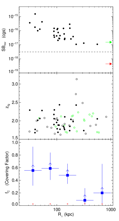
Figure 2.— Properties of projected quasar pair sample. Middle: Distribution of impact parameter and f/g quasar redshift for the 68 projected pairs in our our parent sample. Filled blue circles are 29 sightlines with an optically thick absorber within $|\Delta v|=1500{\rm km~{}s}^{-1}$ of the f/g quasar redshift, which we search for ${\rm Ly\alpha}$ emission (see Table 1). The black open circles are sightlines which are ambiguous, and the green open circles are sightlines classified as optically thin. Bottom: Blue squares show the covering factor of optically thick absorbers in logarithmically spaced bins. Vertical error bars are Poisson. Because some of the ambiguous points (black open circles in middle panel) may also be optically thick, our covering factor is a conservative lower-limit, as denoted by arrows on the blue points. The lower red error bars indicate the expected covering factor within a $|\Delta v|=1500{\rm km~{}s}^{-1}$ interval from the background abundance of LLSs (Ribaudo et al. 2011), with the range given by the current precision of these measurements. The covering factor of optically thick absorbers around quasars is high $>50\%$ for scales $R_{\perp}<200\,{\rm\ kpc}$, and represents a significant enhancement over the cosmological background. Top: Distribution of predicted mirror ${\rm SB}_{\rm mir}$ (eqn. (2.2.2) for the 29 quasars searched for emission. Note the general $R_{\perp}^{-2}$ trend. The dashed line is the median value of the $1\sigma$ SB limits, ${\rm SB}_{1\sigma}$ of our sample. The red arrow indicates the effective $1\sigma$ SB limit of the Rauch et al. (2008) 92 hour integration, where their values are rescaled from $z\simeq 3.1$ to the median redshift of our sample $z=2$ (i.e. $(1+z)^{4}$ dimming) and also rescaled to match our $700\,{\rm km~{}s}^{-1}$ velocity aperture. The green arrow indicates the average SB threshold given the Matsuda et al. (2004) definition of a LAB ($f_{{\rm Ly}\alpha}>0.7{\;\times\;10^{-16}}{\rm erg\ s^{-1}\ cm^{-2}}$ over a 16 arcsec² isophote) also rescaled to $z=2$.

The H I analysis was complemented by a search for metal-lines at the f/g quasar redshift in the clean continuum region redward of the Ly$\alpha$ forest of the b/g quasar. The narrow metal-lines provide a more accurate redshift for the absorption line system (than obtainable from ${\rm Ly\alpha}$) and, if present, they can help distinguish optically thick absorbers from blended Ly$\alpha$ forest lines. We focused on the strongest low-ion transitions commonly observed in DLAs (e.g. Prochaska et al. 2001): Si II $\lambda 1260,1304,1526$, O I $\lambda 1302$, C II $\lambda 1334$, Al II $\lambda 1670$, Fe II $\lambda 1608,2382,2600$, Mg II $\lambda 2796,2803$; and the strong high-ionization transitions commonly seen in LLSs: C IV $\lambda 1548,1550$ and Si IV $\lambda 1393,1402$. Any systems with secure metal-line absorption were also flagged for Voigt profile fitting. Again, this analysis occasionally benefited from the public datasets of SDSS and BOSS whose broad wavelength coverage complements the more limited coverage of our large-aperture spectroscopy.

Given the equivalent width for Ly$\alpha$ absorption, our Voigt profile fits for the $N_{\rm HI}$, and the presence/absence of low-ion metal absorption, objects were classified into three categories: optically thick, ambiguous, or optically thin. Objects which show obvious damping wings or strong (EW $>0.3$ Å) low-ion metal absorption are classified as optically thick. For cases for which metal lines are weak, not covered by our spectral coverage, or significantly blended with the Ly$\alpha$ forest of the b/g quasar, an object is classified as optically thick only if it has $W_{\rm Ly\alpha}$$\geq 1.7$Å. Table 1 lists relevant quantities for the final sample of 29 objects classified as optically thick, around which we search for extended ${\rm Ly\alpha}$ emission.

The false positives and completeness of our optically thick sample are sources of concern. Line-blending, in particular, can significantly depress the continuum near the Ly$\alpha$ profile biasing the $W_{\rm Ly\alpha}$ and the estimated column density high. Based on the analysis of our current sample, and comparisons of objects observed at moderate and echellette/echelle resolution (see e.g. Hennawi et al. 2006a), we estimate that false-positives, that is non optically-thick objects, in our sample is lower than $10\%$. This low contamination follows from our relatively conservative criteria for defining a system as optically thick. Specifically, there are 3 cases for which we are less confident in the optically thick designations (see Table 1; J1041+5630, J1045+4351, J1444+3113) but we nevertheless include them in the following analysis. Removing them would make no difference to our conclusions aside from reducing the sample size by 10%. Note that saturated Ly$\alpha$ forest lines with $N_{\rm HI}<10^{17.2}\,{\rm cm}^{-2}$ are essentially indistinguishable from optically thick absorbers with low-metallicity. As such, we expect the false positive rate to be smaller than our incompleteness, and we thus consider our estimate of the covering factor of optically thick gas (see Figure 2) to be conservative lower limits.

Finally, given that there is suggestive evidence that radio-loud quasars have brighter ${\rm Ly\alpha}$ emission nebulae and a higher detection frequency than radio-quiet quasars (Heckman et al. 1991b), and that HzRGs at $z\sim 2$ typically exhibit bright (${\rm SB}_{{\rm Ly}\alpha}\sim 10^{-16}{\rm\,erg\,s^{-1}\,cm^{-2}\,arcsec^{-2}}$) large-scale ($\sim 100\,{\rm\ kpc}$) ${\rm Ly\alpha}$ nebulae (e.g. McCarthy et al. 1990; McCarthy 1993; van Ojik et al. 1996; Nesvadba et al. 2006; Binette et al. 2006; Reuland et al. 2007; Villar-Martín et al. 2007; Miley & De Breuck 2008), we consider the radio properties of our f/g quasars. The Faint Images of the Radio Sky at Twenty cm survey (FIRST; Becker et al. 1995) used the Very Large Array (VLA) to produce a map of the 20 cm (1.4 GHz) sky with a beam size of $5.^{\prime\prime}4$ and an rms sensitivity of about 0.15 mJy beam^-1. The survey covers the same 10,000 deg² sky region covered by the SDSS imaging, has a typical detection threshold of 1 mJy, and an astrometric accuracy of $0.05^{\prime\prime}$. Following (Ivezić et al. 2002), we match our f/g quasars to the FIRST catalog with a matching radius of $1.5^{\prime\prime}$. From our parent sample of 68 projected pairs, only 59 sources were covered by the FIRST imaging footprint, and of these, 4/59 have matches in the FIRST catalog ($F_{\rm peak}\gtrsim 1\,{\rm mJy}$), which is consistent with roughly $\sim 10\%$ of quasars being radio-loud (Ivezić et al. 2002). This is to be expected since our f/g quasars are typical SDSS quasars. Visual inspection of the FIRST images indicates that none show evidence of a complex radio morphology (i.e. core-jet, core-lobe, and double-lobe; Magliocchetti et al. 1998; McMahon et al. 2002). Among the 29 f/g quasars with coincident optically thick absorption, 28 sources were covered by the FIRST footprint, and only 3/28 have matches in the FIRST catalog, again consistent with a $\sim 10\%$ radio loud fraction. The radio fluxes for the three sources detected in the FIRST survey are listed in in Table 1; for the sources which were not detected we list 5$\sigma$ upper limits based on the FIRST sky-rms coverage maps. Given that only $\sim 10\%$ of our f/g quasars have radio counterparts $\gtrsim 1\,{\rm mJy}$, both in our parent sample and in the sample with coincident absorbers, we conclude that quasars which we study here are predominantly radio-quiet.

3.4. The Covering Factor of Optically Thick Absorbers

The distribution of f/g quasar redshifts and transverse separations for all 68 projected quasar pair sightlines in our parent sample are shown in the scatter plot in Figure 2. The 29 black filled symbols indicate sightlines which have an optically thick absorber within an interval $\delta v=[-1500,1500]\,{\rm km~{}s}^{-1}$ of the f/g quasar redshift (the median absolute offset of these systems is $|\delta v|=256\,{\rm km~{}s}^{-1}$), which are objects that we search around for extended ${\rm Ly\alpha}$ emission. Open black circles indicate sightlines classified as ambiguous, and green sightlines which are optically thin. Note that the closest pairs are predominantly at redshift $z\sim 2$, because this is where quasar selection, and hence quasar pair selection, is most efficient (see Richards et al. 2002a; Hennawi et al. 2006b; Bovy et al. 2011, 2012).

It is clear from Figure 2 that the covering factor of absorbers is very high for small separations: at least 28 out of 48 sightlines with $R_{\perp}<200$ kpc have signatures of optically thick gas coincident with the f/g quasar, implying a $>58\%$ covering fraction. This high covering factor was previously noted in Hennawi et al. (2006a) based on a much smaller pair sample (11 sightlines with $R_{\rm perp}<200\,{\rm\ kpc}$) which are a subset of our current parent sample (see also QPQ5). Note again that because of the significant incompleteness discussed in §3.3, this high covering factor should be interpreted as a conservative lower limit, albeit subject to Poisson uncertainty.

The distribution of points in Figure 2, or equivalently the dependence of covering factor on impact parameter, can be used to measure the quasar-absorber correlation function, which is equivalently the spatial profile of the absorbing clouds around the f/g quasar. In QPQ2, we analyzed the much smaller sample of pairs from QPQ1 and determined a correlation length of $r_{0}=9.2^{+1.5}_{-1.7}~{}h^{-1}{\rm\ Mpc}$ (comoving) assuming a power law correlation function, $\xi\propto r^{-\gamma}$, with $\gamma=1.6$. The high covering factor of absorbers quantified by the correlation function, implies a comparably high incidence of proximate absorbers along the line-of-sight; however, this absorption is not observed in our f/g quasars, or in other isolated quasars. This anisotropic clustering of absorbers around quasars indicates that the transverse direction is less likely to be illuminated by ionizing photons than the line-of-sight, either because of anisotropic emission which could result if the f/g quasar is obscured from some vantage points, or because the quasar emits radiation intermittently, on a timescale comparable to the transverse light-crossing time. We will return to this important inference in the context of the search for ${\rm Ly\alpha}$ fluorescence in §5.

4. Data Reduction and PSF Subtraction

Our goal is to conduct a sensitive search for extended ${\rm Ly\alpha}$ emission in slit spectra in the CGM region surrounding the f/g quasar in quasar pairs. Our approach is to subtract off the point spread function (PSF) of the the quasars and other objects (galaxies or stars), which may have serendipitously landed on the slit, and search for resolved ${\rm Ly\alpha}$ emission which is inconsistent with these spectral PSFs. In the next sections, we describe the details of our data reduction and spectral PSF subtraction algorithm, our procedure for flux calibration and determining surface brightness limits, and our simulation using synthetic sources to determine the surface brightness levels we can visually detect.

4.1. Data Reduction and PSF Subtraction Algorithm

The Gemini/GMOS observations were conducted in longslit mode, whereas the LRIS observations include a mix of longslit and multislit exposures. All data were reduced using the LowRedux pipeline, which is a publicly available collection of custom codes written in the Interactive Data Language (IDL) for reducing slit spectroscopy. Individual exposures are processed using standard techniques, namely they are overscan and bias subtracted and flat fielded. Flat fielding is performed in two steps, using both a pixel flat to correct for pixel-to-pixel sensitivity variations, as well as spectroscopic illumination flats (taken with the sky in twilight) to flatten the larger scale illumination pattern arising from either instrument optics or imperfections in the slits. Cosmic rays and bad pixels are identified and masked in multiple steps. First, a sharpness detection algorithm is run on each image to identify and mask features smaller than the spectral/spatial PSF. Then further downstream in the reduction procedure, outliers from our models of the sky and the object are masked (see below). Wavelength solutions are determined from low order polynomial fits to arc lamp spectra, and then a wavelength map is obtained by tracing the spatial trajectory of arc lines across each slit. This wavelength map allows us to model the sky counts as a function of wavelength and slit position without needing to rectify the original data (e.g. Kelson 2003).

Our method for spectral PSF subtraction employs a novel custom algorithm. We treat sky and PSF subtraction as a coupled problem to obtain a multi-component model of the image counts. This model is composed of a sum of 2-d ‘basis functions’, which consists of a sky background and a PSF model for each object on the slit. This is typically just the two quasars (f/g and b/g), but in some cases it includes additional objects which landed on the slit in the region of interest. By construction, the sky-background has a flat spatial profile because our slits are flattened by the slit illumination function. For the object models, we first identify objects in an initial sky-subtracted image, and trace their trajectory across the detector. We then extract a 1-d spectrum, normalize these sky-subtracted images by the total extracted flux, and fit a B-spline profile to the normalized spatial light profile of each object relative to the position of its trace. This non-parametric object profile has the flexibility to vary as a function of wavelength, and corrections to the initial trace are simultaneously determined and applied. Given this set of 2-d basis functions, i.e. the flat sky and the object model profiles, we then minimize chi-squared for the best set of spectral B-spline coefficients (i.e. break points are spaced in wavelength) which are the spectral amplitudes of each basis component of the 2-d model. In other words

$$\chi^{2}=\sum_{i}^{N_{\rm pix}}\frac{\left({\rm DATA}_{i}-{\rm MODEL}_{i}\right)^{2}}{\sigma_{i}^{2}}$$ (21)

where the sum is taken over all $N_{\rm pix}$ pixels in the image, ‘DATA’ is the image, ‘MODEL’ is a linear combination of 2-d basis functions multiplied by B-spline spectral amplitudes, and $\sigma$ is a model of the noise in the spectrum, i.e. $\sigma^{2}={\rm SKY}+{\rm OBJECTS}+{\rm READNOISE}$. The result of this procedure are then full 2-d models of the sky-background (SKY), all object spectra (OBJECTS), and the noise ($\sigma^{2}$). We then use this model SKY to update the sky-subtraction, the individual object profiles are re-fit and the basis functions updated, and chi-square fitting is repeated. We iterate this procedure of object profile fitting and subsequent chi-squared modeling four times until we arrive at our final models for the sky background, the 2-d spectrum of each object, and the noise.

Each exposure of a given target is modeled according to the above procedure which then allows us to subtract the sky and the object profiles from each individual image. These images are registered to a common frame by applying integer pixel shifts (to avoid correlating errors), and are then combined to form final 2-d stacked sky-subtracted and sky-and-PSF-subtracted images. The individual 2-d frames are optimally weighted by the ${\rm(S/N)}^{2}$ of their extracted 1-d spectra (using the b/g quasar), and bad pixels identified via sharpness filtering, as outliers in the chi-square fitting, or by sigma-clipping of the image stack, are masked. The final result of our data analysis are three images: 1) an optimally weighted average of $({\rm DATA}-{\rm SKY})$, henceforth the ‘stacked sky-subtracted image’, 2) an optimally weighted average of $({\rm DATA}-{\rm SKY}-{\rm OBJECTS})$, henceforth the ‘stacked sky-and-PSF-subtracted image’, and 3) the noise model for these images $\sigma^{2}$. The final noise map is propagated from the individual noise model images taking into account weighting and pixel masking entirely self-consistently.

Extended ${\rm Ly\alpha}$ emission will be manifest as residual flux in our 2-d sky-and-PSF-subtracted images which is inconsistent with being noise. We thus search for ${\rm Ly\alpha}$ emission by defining a $\chi$ image in analogy with eqn. (21) above, but using the stacked images and corresponding propagated noise instead of the individual frames. This procedure allows us to visually assess the statistical significance of any putative emission feature. Figure 5 presents these images for the 29 objects in our optically thick sample (see Table 1). The middle panels show $\chi_{\rm sky+PSF}=({\rm DATA}-{\rm SKY}-{\rm OBJECTS})/\sigma$ for the stacked sky-and-PSF-subtracted images. Recall that an analogous $\chi^{2}$ has been minimized by our modeling of each image. Thus if our model is an accurate description of the data, the distribution of pixel values in the $\chi_{\rm sky+PSF}$ should be a Gaussian with unit variance. The lower panel of each image shows $\chi_{\rm sky}=({\rm DATA}-{\rm SKY})/\sigma$; the numerator is the the stacked sky-subtracted (but not PSF-subtracted) image. The upper panels show smoothed maps which are helpful for identifying extended emission. Specifically, the smoothed images are given by

$$\chi_{\rm smth}=\frac{{\rm CONVOL}[{\rm DATA}-{\rm SKY}-{\rm OBJECTS}]}{{\rm CONVOL}[\sigma]},$$ (22)

where the ${\rm CONVOL}$ operation denotes smoothing of the stacked images with a symmetric Gaussian kernel (same spatial and spectral widths) with FWHM${}_{\rm smth}=235\,{\rm km~{}s}^{-1}$ (dispersion $\sigma_{\rm smth}=100\,{\rm km~{}s}^{-1}$). For LRIS this FWHM_smth corresponds to 5.2-6.1 pixels, or 1.4-1.5 times the spectral resolution element, and $1.4-1.6^{\prime\prime}$ spatially. For GMOS a FWHM${}_{\rm smth}=235\,{\rm km~{}s}^{-1}$ corresponds to 6.6-7.0 pixels or 1.4-1.5 times the spectral resolution, or $1.9-2.0^{\prime\prime}$ spatially.

Note that smoothing correlates pixels in the smoothed image, and furthermore the ratio of smoothed image to smoothed noise will no longer obey Gaussian statistics. Nevertheless, $\chi_{\rm smth}$ proves to be a useful tool for identifying extended emission.

4.2. Flux Calibration and Surface Brightness Limits

The following describes our procedure to flux calibrate our spectra and determine surface brightness limits. Standard star spectra were not typically taken immediately before/after our quasar pair observations. Instead, we construct a model sensitivity function of the Keck LRIS-B spectrograph by first fitting an aggregate of standard star spectra taken at different slit positions, which span the range of wavelength coverage available with a multi-slit setup. A similar procedure was employed for Gemini GMOS using standard star spectra taken at a variety of central wavelengths. We apply this archived sensitivity function to the b/g quasar spectrum, and then integrate the flux-calibrated 1-d spectrum against the SDSS $u$-band filter curve. The sensitivity function is then rescaled to yield the correct SDSS $u$-band photometry. A comparison of our 1-d spectra flux calibrated in this way to the SDSS spectra typically show agreement to within $\sim 10-20\%$ in the region of wavelength overlap. Given that SDSS spectra have spectrophotometric errors of $\sim 10\%$ (Abazajian et al. 2005), that $u$-band photometric errors (used for our renormalization) are about $7\%$ for a typical source with $u\simeq 21$, and that quasar variability over $\simeq 5$ year timescales (between when the SDSS photometry and our spectra were taken) could result in a $\sim 10\%$ fluctuation (e.g. Schmidt et al. 2010), we consider $\sim 20\%$ agreement between our spectra and the SDSS spectra to be reasonable.

This procedure of rescaling the sensitivity functions to match photometry is effective for point source flux-calibration, however a subtlety arises in relation to calibrating extended emission. The point source counts will be reduced because of improper object centering due to guiding errors or inaccuracies in slit/mask alignment, and because a fraction of the spatial PSF lies outside the slit area. These point-source slit-losses do not, however, reduce the amount of spatially resolved emission, which is of interest here. Thus, renormalizing to point-source photometry will tend to over-estimate our surface brightness detection limit and underestimate our sensitivity. Hence, our procedure is to apply the rescaled sensitivity functions (based on point source photometry) to our 2-d images, but reduce them by a geometric slit-loss factor so that we properly treat extended emission.

To compute the slit-losses we use the measured spatial FWHM to determine the fraction of light going through our $1.0^{\prime\prime}$ slits, but we do not model centering errors. A useful check on our flux calibration procedure is to examine any residual variation in our renormalized sensitivity functions after the effects of the atmospheric extinction (i.e. due to airmass) and slit-losses are removed. These variations in the spectroscopic zero-point could be due either to transparency variations or to other systematic flux calibration errors. We find a 35% relative variation ($1\sigma$) about the mean zero-point, which is at a level that can be plausibly explained by transparency variations in clear but non-photometric conditions. If these variations in zero-point are indeed due to transparency fluctuations, then our procedure of renormalizing to the photometry effectively takes them out. But because we have no quantitative information about the transparency during our observations, we conservatively assume a relative error of $\sim 35\%$ on our surface brightness limits.

Application of the wavelength dependent sensitivity function converts our stacked sky-and-PSF-subtracted images from units of electrons into ${\rm erg\,s^{-1}\,cm^{-2}}\,$Å^-1. We then tile these calibrated images with a uniform grid of aperture centers within $\pm 3000\,{\rm km~{}s}^{-1}$ of the f/g quasar’s redshifted ${\rm Ly\alpha}$ line. Regions within $\pm 7.0^{\prime\prime}$ of the f/g quasar trace on either side are excluded to avoid potential contamination from ${\rm Ly\alpha}$ emission. Regions within $\pm 3000\,{\rm km~{}s}^{-1}$ of the b/g quasar’s ${\rm Ly\alpha}$ and also within $\pm 7.0^{\prime\prime}$ of the b/g quasar trace are also excluded, to similarly avoid ${\rm Ly\alpha}$ contamination (this is relevant if the redshift difference of the pair $\delta v<3000\,{\rm km~{}s}^{-1}$). The spacing between these aperture centers is 1.0^′′ spatially and $\Delta v=400\,{\rm km~{}s}^{-1}$ spectrally. We then compute SB limits in windows of $700\,{\rm km\,s^{-1}}\!\times 1.0^{\prime\prime}$ about each aperture center, which corresponds to an aperture of $700\,{\rm km\,s^{-1}}\!\times 1.0\,{\rm arcsec}^{2}$ on the sky because we always used a $1.0^{\prime\prime}$ slit. The $700\,{\rm km~{}s}^{-1}$ spectral width is motivated by the observed kinematics of the metal-line absorbers associated with the optically thick gas we detect in absorption (Prochaska & Hennawi 2009, Prochaska et al.  in prep.). If this gas emits ${\rm Ly\alpha}$, we expect the emission kinematics to have a comparable velocity width (in the absence of significant resonant broadening). Because our noise has been propagated self-consistently, we use the noise model for our stacked sky-and-PSF-subtracted image to determine the 1$\sigma$ surface brightness limit for the $i$th aperture ${\rm SB}_{1\sigma,i}$, and we take the mean value of $1/N\sum_{i}^{N}{\rm SB}_{1\sigma,i}$ of all apertures to be the surface brightness limit for the quasar pair ${\rm SB}_{1\sigma}$, which is quoted in Table 1.

We can assess the accuracy of our noise model by examining the distribution of $\chi_{i}={\rm SB}_{i}/{\rm SB}_{1\sigma,i}$, where ${\rm SB}_{i}$ is the extracted flux of the $i$th aperture in each $700\,{\rm km\,s^{-1}}\times 1.0\,{\rm arcsec}^{2}$ window, and ${\rm SB}_{1\sigma,i}$ is the surface brightness limit based on our noise model at this location. In the absence of detectable extended ${\rm Ly\alpha}$ emission the ${\rm SB}_{i}$ should be pure noise, and if our noise model is accurate, the $\chi_{i}$ should thus obey a Gaussian distribution with unit variance. The distribution of $\chi_{i}$ for one of our quasar pairs SDSSJ 0938$+$5317 is compared to a Gaussian in Figure 3. It is clear that our noise model provides an accurate description of the real noise in the stacked sky-and-PSF subtracted image. Systematic errors in the data reduction and sky and object modeling procedure are not accounted for in the purely statistical error ${\rm SB}_{1\sigma,i}$, and thus we would expect to typically underestimate the true noise level. We can quantify these errors in our noise estimates by computing the standard deviation of $\chi_{i}$ after clipping $>5\sigma$ outliers (resulting from e.g. a small number of residual cosmic ray hits or bad pixels that remain unmasked by our data reduction procedure). For the distribution in Figure 3 we obtain $\sigma_{\rm chi}=0.97$, which indicates that for this case we actually slightly overestimated the noise. We similarly compute $\sigma_{\rm chi}$ for each quasar pair in our sample. The median value over all quasar pairs is 1.08, thus on average we tend to underestimate the noise by $8\%$. Because this is smaller than our estimated flux calibration error, we therefore quote statistical SB limits based only on our noise model as ${\rm SB}_{1\sigma}$ in Table 1.

4.3. Visually Recovering Synthetic Sources

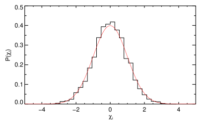
Figure 3.— Distribution of extracted surface brightness apertures relative to noise model predictions. The histogram shows the distribution $\chi_{i}={\rm SB}_{i}/{\rm SB}_{1\sigma,i}$ for one of our sources SDSSJ 0938$+$5317 from Figure 5. In the absence of detectable extended ${\rm Ly\alpha}$ emission the ${\rm SB_{i}}$ should be pure noise, and if our noise model is accurate, then $\chi_{i}$ should follow a Gaussian distribution with unit variance, which is shown by the solid red curve. The standard deviation of $\chi_{i}$ after clipping $>5\sigma$ outliers is $\sigma_{\rm chi}=0.97$, which indicates that our noise model is indeed accurate and that fluctuations obey Gaussian statistics as expected. The median value of $\sigma_{\rm chi}$, computed similarly, over all of our quasar pairs is 1.08, indicating that on average we tend to underestimate the noise by $8\%$.

Figure 4.— Illustration of detection significance of synthetic sources with various properties. The lower panel shows the $\chi_{\rm skyonly}$ image for SDSSJ 0938$+$5317 with synthetic sources added according to the procedure described in §4.3. In only the lower panel, the synthetic sources are noiseless, and their brightness and relative significance can be directly compared to the real (noisy) spectra of the two quasars shown in the central inset. The middle and upper panels show $\chi_{\rm sky+object}$ and $\chi_{\rm smth}$ images respectively, which are the same as the corresponding panels for SDSSJ 0938$+$5317 in Figure 5, except that noisy synthetic sources have been added. The stretch and colormap are identical to that used for all of our $\chi$ maps in Figure 5, and is indicated by the upper colorbar. The horizontal red and blue dashed lines and the vertical red dotted line are the same as in Figure 5. The colored circles indicate the location of the sources for various significance levels which are labeled in black at the top of the bottom panel. The red circles indicate the large ’CGM’ sources which are both spectrally and spatially resolved, black circles the ’LLS’ sources which are spatially resolved but spectrally unresolved, and blue circles the ’CORE’ sources which are both spatially and spectrally unresolved. This figure suggests that we should be able to marginally detect ’CGM’ like sources that are $\gtrsim 2\times{\rm SB}_{1\sigma}$, ’LLS’ like emission with $\gtrsim 3\times{\rm SB}_{1\sigma}$, and ’CORE like sources to $\gtrsim 10\times{\rm SB}_{1\sigma}$. Note that the blob of emission near $\Delta v=0\,{\rm km~{}s}^{-1}$ and impact parameter $R_{\perp}\approx-20\,{\rm\ kpc}$ is real small-scale Ly$\alpha$ fuzz emission from the f/g quasar (see §5.2).

Having quantified the formal errors in our sky-and-PSF-subtracted images, we now determine the significance level for a convincing detection. While we quote $1\sigma$ SB limits over $700\,{\rm km\,s^{-1}}\times 1.0\,{\rm arcsec}^{2}$ apertures, our sensitivity to a given surface brightness is of course set by the size of the source and its spectral characteristics (i.e. kinematics). One can in principle always reach lower SB levels by averaging over larger spatial regions, and it is easier to detect narrow lines over the background. To address these issues we construct synthetic fluorescent sources and add them to the sky-and-PSF-subtracted image for a representative pair SDSSJ 0938$+$5317. This pair has $z_{\rm bg}=2.32$, $z_{\rm fg}=2.07$, an angular separation of $\theta=5.6^{\prime\prime}$ corresponding to $R_{\perp}=49\,{\rm kpc}$, and was observed with LRIS, as are the bulk of our pairs. The total exposure time was 1800s, allowing us to reach a surface brightness limit of ${\rm SB}_{1\sigma}=0.29{\;\times\;10^{-17}}{\rm\,erg\,s^{-1}\,cm^{-2}\,arcsec^{-2}}$ which is close to the median value of our sample ${\rm SB}_{1\sigma}=0.31{\;\times\;10^{-17}}{\rm\,erg\,s^{-1}\,cm^{-2}\,arcsec^{-2}}$ (Table 1). Figure 3 testifies to the accuracy of our noise model for this object, and illustrates that the surface brightness noise fluctuations obey Gaussian statistics. Our spectral resolution for these observations is FWHM$=153\,{\rm km~{}s}^{-1}$ and the seeing measured from the quasar profiles is $0.79^{\prime\prime}$ corresponding to a spatial resolution of $7.0\,{\rm\ kpc}$.

We construct synthetic sources with a uniform spatial surface brightness distribution, where the size is specified by a single dimension along the slit $d_{\rm fake}$. Spectrally, we assume a Gaussian velocity profile specified by FWHM_fake. The amplitude of the synthetic sources is set such that their total surface brightness (i.e. integrated out spectrally) is equal to ${\rm SB}=[1,2,3,4,5,10]\times{\rm SB}_{1\sigma}$, which corresponds to ${\rm SB}_{{\rm Ly}\alpha}=[0.29,0.57,0.86,1.1,1.4,2.9]{\;\times\;10^{-17}}\,{\rm\,erg\,s^{-1}\,cm^{-2}}$ ${\rm arcsec^{-2}}$ for SDSSJ 0938$+$5317.

We consider synthetic sources with three different spatial and kinematic distributions which represent our expectations for the sources that might occur near a bright quasar. The first is a large $d_{\rm fake}=75\,{\rm\ kpc}$ source with kinematics FWHM${}_{\rm fake}=500\,{\rm km~{}s}^{-1}$, which is both spatially and spectrally resolved. This source represents the kind of emission expected if the quasar CGM is made up of a large population of small spatially unresolved clouds which nevertheless have sufficient covering factor, $f_{\rm C}$, to result in detectable ${\rm Ly\alpha}$ emission (see Figure 1b-d); we denote this model as ‘CGM’. In this scenario, the kinematics of the emission correspond to the motions traced by the metal-line absorbers as observed near quasars with b/g sightlines (Prochaska & Hennawi 2009, Prochaska et al., in prep.). The second synthetic source is meant to represent a spatially resolved ${\rm Ly\alpha}$ source (see Figure 1a), which is the counterpart to the frequently observed optically thick absorption in b/g quasar sightlines (Figure 2). In this ‘LLS’ scenario, the size is taken to be $d_{\rm fake}=20\,{\rm kpc}$, corresponding to about three resolution elements. The kinematics are assumed to be comparable to the narrow turbulent and/or thermally broadened line widths $\sim 20\,{\rm km~{}s}^{-1}$ characteristic of metal absorption in individual LLS absorption complexes, (i.e., spectrally unresolved Prochter et al. 2010). For the third synthetic source, denoted as ‘CORE’, we assume a size $d_{\rm fake}$ of two LRIS pixels corresponding to $4.8\,{\rm\ kpc}$, and cold kinematics $\sim 20\,{\rm km~{}s}^{-1}$, such that it is both spatially and spectrally unresolved. This source is meant to mimic the properties of the candidate fluorescent emitters recently detected by Cantalupo et al. (2012) at $\sim$ Mpc distances from bright quasars. These fluorescent candidates tend to be compact, are spatially unresolved in ground-based seeing, and are believed to be the dense cores of proto-galaxies. For spatially unresolved sources, the total ${\rm Ly\alpha}$ luminosity is the relevant quantity rather than the surface brightness, and the corresponding luminosity of our CORE sources are $L_{{\rm Ly}\alpha}=[0.92,1.8,2.8,3.7,4.6,9.2]{\;\times\;10^{41}}\,{\rm\,erg\,s^{-1}}$. Note that the median luminosity for the most compelling (i.e. those with $W_{{\rm Ly}\alpha}>240$Å) Cantalupo et al. (2012) fluorescent candidates is $L_{{\rm Ly}\alpha}=9.1\,{\;\times\;10^{41}}\,{\rm\,erg\,s^{-1}}$, which is at the level of the 10$\sigma$ model source we consider. Our model images are then convolved with the spectral and spatial resolution of our data, converted into counts using our sensitivity function, and Poisson realizations of the average counts are added to the real sky-subtracted and sky-and-PSF-subtracted images.

Figure 4 illustrates the detection significance of the synthetic source model profiles which have been added to the real data for SDSSJ 0938$+$5317. The lower panel shows the $\chi_{\rm sky}$ with synthetic sources added. In this panel only, the synthetic sources are noiseless, and their brightness and relative significance can be directly compared to the real (noisy) 2-d spectra of the two quasars shown in the central inset. Quantitatively, a uniform screen of surface brightness at ${\rm SB}_{1\sigma}=0.29{\;\times\;10^{-17}}{\rm\,erg\,s^{-1}\,cm^{-2}\,arcsec^{-2}}$ emitted at the f/g quasar ${\rm Ly\alpha}$ with a top-hat velocity distribution matched to our $700\,{\rm km~{}s}^{-1}$ spectral extraction aperture would result in $0.44\,e^{-}$ electrons per pixel, whereas the typical value of the $1\sigma$ noise in our stacked images (far from the quasars) is $\sigma\simeq 4\,e^{-}$ electrons per pixel.

Inspection of Figure 4 suggests that we should be able to marginally detect ‘CGM’ like sources down to a level of $\gtrsim 2\times{\rm SB}_{1\sigma}$, ‘LLS’ like sources down to $\gtrsim 3\times{\rm SB}_{1\sigma}$, and the spatially and spectrally unresolved ‘CORE’ like sources to $\gtrsim 10\times{\rm SB}_{1\sigma}$. We emphasize that these significance limits are rough guidelines, as the noise level varies with wavelength due to fluctuations in the sky level. For example, the reason why the $4\sigma$ sources in Figure 4 look scarcely more significant than the $3\sigma$ ones, is that the $4\sigma$ sources happen to land on a region where the sky-background is $\sim 10\%$ higher. Furthermore, in some cases systematics in the data reduction limit our ability to make detections down to low significance levels. These systematics manifest as large-scale correlations in the $\chi$ maps, and are particularly conspicuous in the smoothed $\chi_{\rm smth}$ images. In the absence of emission, the $\chi_{\rm sky+object}$ image should be a random Poisson noise field because the pixel noise is completely uncorrelated, and thus the characteristic size of structures in the $\chi_{\rm smth}$ should be comparable to the size of the smoothing kernel $\simeq 5-6$ pixels. Some of our $\chi$ maps in Figure 5 show correlated structure and spurious features due to systematics, the worst case being SDSSJ 0814$+$3250, where a large-scale gradient in the flux level is seen across the spatial direction. This large-scale gradient is likely due to a poorly determined slit-illumination function.

5. Results and Discussion

In what follows we interpret our observational results from the previous section in terms of the emission mechanisms discussed in §2. The results further constrain the physical properties of the CGM of the massive galaxies hosting $z\sim 2$ quasars. Before delving into details, we briefly summarize the main findings of our search for ${\rm Ly\alpha}$ emission in the regions surrounding quasars. Careful inspection of the ${\rm Ly\alpha}$ emission maps in Figure 5 reveals the following:

• Fluorescent ${\rm Ly\alpha}$ emission with properties expected in the ‘mirror’ approximation, is not detected at the locations of optically thick absorbers pinpointed by the b/g quasar sightlines.

• Despite the fact that the covering factor of optically thick absorbers on scales $R_{\perp}\sim 100\,{{\rm\ kpc}}$ is high ($f_{\rm C}>0.5$), we do not detect diffuse ${\rm Ly\alpha}$ emission on these large scales, with the exception of a single system.

• In a single system SDSSJ 0841$+$3921, we detect a spectacular ${\rm Ly\alpha}$ filament around the foreground quasar with surface brightness ${\rm SB}\simeq 1{\;\times\;10^{-17}}{\rm\,erg\,s^{-1}\,cm^{-2}\,arcsec^{-2}}$ and an extent of 230  kpc and possibly as large as 330  kpc(discussed further in Hennawi et al.  in prep.).

• Extended ${\rm Ly\alpha}$ fuzz is frequently detected on small-scales $R_{\perp}<50\,{\rm\ kpc}$. We detect definite fuzz in 10 objects, or 34% of our sample, at levels of ${\rm SB}_{{\rm Ly}\alpha}\simeq 0.5-5{\;\times\;10^{-17}}{\rm\,erg\,s^{-1}\,cm^{-2}\,arcsec^{-2}}$.

• In SDSSJ 0856$+$1158, a high-equivalent width ($W_{{\rm Ly}\alpha}>50$Å; rest-frame) Ly$\alpha$-emitter is detected with $L_{{\rm Ly}\alpha}=2.1\pm 0.32{\;\times\;10^{41}}{\rm\,erg\,s^{-1}}$, at a distance of $134\,{\rm\ kpc}$ and velocity $-540\,{{\rm km~{}s}^{-1}}$ relative to the f/g quasar.

As we will frequently refer to our observations in aggregate, for reference we list the typical properties of our sample of 29 projected quasar pair observations. The median redshift of our f/g quasars is $z_{\rm fg}=1.95$, which are probed by b/g sightlines at a median impact parameter of $R_{\perp}=106\,{\rm\ kpc}$. The luminosity at the Lyman limit has a median value $\log_{10}L_{\nu_{\rm LL}}\simeq 30.3$ and our f/g quasars have a median de-reddened $i$-band apparent magnitude of 19.7. Our median $1\sigma$ ${\rm Ly\alpha}$ surface brightness is ${\rm SB}_{1\sigma}=0.31{\;\times\;10^{-17}}{\rm\,erg\,s^{-1}\,cm^{-2}\,arcsec^{-2}}$, and according to the example in §4.3, large scale emission from the quasar CGM should be detectable for $\gtrsim 2\times{\rm SB}_{1\sigma}$ or ${\rm SB}_{{\rm Ly}\alpha}\gtrsim 0.6{\;\times\;10^{-17}}{\rm\,erg\,s^{-1}\,cm^{-2}\,arcsec^{-2}}$.

5.1. Fluorescent Emission from Optically Thick Gas

In this subsection we compare our observational constraints on extended ${\rm Ly\alpha}$ emission to predictions for recombination radiation from optically thick gas, as laid out in §2.2.2. We consider emission from spatially resolved ‘mirrors’ and from an unresolved distribution of clouds in turn.

5.1.1 Fluorescent Emission in the Mirror Approximation

The frequent detection of optically thick gas in the CGM of quasars quantified in §3.4, and discussed in other work in the QPQ series (Hennawi et al. 2006a; Hennawi & Prochaska 2007; Prochaska et al. 2012, 2013), provided initial optimism that we would detect significant fluorescent ${\rm Ly\alpha}$ emission from this population of clouds. In the simple ‘mirror’ approximation (see eqn. 2.2.2; Gould & Weinberg 1996), $\approx 60\%$ of the ionizing photons impinging on an optically thick cloud are converted into ${\rm Ly\alpha}$ photons, which may be ‘reflected’ into our line-of-sight. A precise estimate of the surface brightness depends on the ionizing photon flux, the cloud size, the geometrical configuration between the source, observer, and cloud(s), as well as the velocity field (Cantalupo et al. 2005; Kollmeier et al. 2008). For spatially resolved clouds (see Figure 1a), the ${\rm Ly\alpha}$ emission should also be spatially resolved and emerge from the side of the absorber that lies closest to the quasar at a SB level given by eqn. (2.2.2). The predicted ${\rm SB}_{\rm mirror}$ values are given for each pair in Table 1, where the distance is taken to be the impact parameter $R_{\perp}$ to the b/g sightline.

Adelberger et al. (2006) purported to detect ${\rm Ly\alpha}$ fluorescence from a serendipitously discovered DLA ($\log N_{\rm HI}=20.4$) situated $49^{\prime\prime}$ away from a luminous quasar at $z=2.84$. The ionizing flux at transverse distance $R_{\perp}=384~{}{\rm kpc}$ implies a very high mirror surface brightness of ${\rm SB}_{\rm mirror}=1.1{\;\times\;10^{-16}}{\rm\,erg\,s^{-1}\,cm^{-2}\,arcsec^{-2}}$ in this system, owing to the extremely luminous foreground quasar ($r\simeq 16$). The authors detect a marginally resolved emission-line source near the b/g sightline with comparable surface brightness; and based on this agreement, the presence of a double-peaked kinematic emission line profile, the small spatial separation ($1.5^{\prime\prime}$ or $11{\rm\ kpc}$) of the emission from the DLA (and b/g sightline), and importantly, the fact that the emission is on the side of the absorber closest to the f/g quasar, they argue that it is ${\rm Ly\alpha}$ fluorescence from the same gas responsible for the DLA absorption.

Here we have conducted a similar search for analogous ‘mirror’ fluorescent emission from a much enlarged sample of 29 sightlines with the same experimental setup as Adelberger et al. (2006). In 24/29 of these sightlines we could have detected emission similar to Adelberger et al. (2006) at $>10\sigma$ (see Table 1), but fail to detect anything comparable. As discussed in §4.3, resolved sources with size $\simeq 20\,{\rm kpc}$, should be detectable down to the level corresponding to $2\times{\rm SB}_{1\sigma}$. With the exception of SDSSJ 0841$+$3921, which we discuss further in Hennawi et al. (in prep.), we do not detect any emission in the immediate vicinity of the b/g quasar sightlines, as would be expected if the absorbing clouds were spatially resolved ${\rm Ly\alpha}$ mirrors, although we had the sensitivity to detect 24/29 sources at $>10\sigma$. Based on this large number of null detections of mirror fluorescence, we conclude that the purported detection of Adelberger et al. (2006) is most likely the coincidence between a DLA and a star-forming galaxy, and was incorrectly interpreted as ${\rm Ly\alpha}$ fluorescence. Indeed, the ${\rm Ly\alpha}$ emission in this source coincides with the location of a continuum source and the corresponding rest-frame equivalent width of only $75$Å is well within the range produced by conventional stellar populations (i.e. $<240$Å), and is hence entirely consistent with being powered by star-formation. It is possible that the ${\rm Ly\alpha}$ emission in this object is boosted by a fluorescent contribution, an effect also discussed in Cantalupo et al. (2012), but given its relatively low rest-frame equivalent width, and our large sample of similar null detections, any interpretation of the Adelberger et al. (2006) object as ${\rm Ly\alpha}$ fluorescence is entirely speculative.

5.1.2 Fluorescent Emission from Unresolved Clouds

For unresolved optically thick clouds distributed around the quasar (see Figure 1b-d), the fluorescent emission will be manifest as an extended and spatially resolved ‘fuzz’, similar to the large ${\rm Ly\alpha}$ nebulae observed in HzRGs and ${\rm Ly\alpha}$ blobs. In this case, the average surface brightness is given by eqn. (2.2.2). Given the high $f_{\rm C}\gtrsim 0.50$ covering factor of optically thick gas at distances $\lesssim 200\,{\rm kpc}$ (see Figure 2; Prochaska et al. 2012), the expected surface brightness of such nebulae is about $\simeq 30\%$ smaller than the mirror values tabulated in Table 1 averaged over an aperture $R_{\perp}$. However a $R_{\perp}^{-2}$ profile is expected for the idealized case of a uniform distribution in a spherical halo (see eqn. 2.2.2), and hence the emission would be brighter closer to the quasar. We emphasize that if the optically thick gas giving rise to the high covering factor is illuminated by the f/g quasar, the expectation is that a SB comparable to the mirror sufrace brightness is expected at impact parameters $R_{\perp}\lesssim 200\,{\rm\ kpc}$ all along the slit (see Figure 1).

Such large-scale diffuse ${\rm Ly\alpha}$ halos would have been very easy to detect. Indeed our CGM synthetic source simulation with emission extending over $70\,{\rm\ kpc}$ (see $\S$ 4.3 and Figure 4) indicates that we could have detected such resolved emission at levels ${\rm SB_{{\rm Ly}\alpha}}\gtrsim 2\times{\rm SB}_{1\sigma}$. Assuming a fixed distance $R=100\,{\rm\ kpc}$ and a covering factor of $f_{\rm C}=0.50$, consistent with our measurements in Figure 2, the optically thick surface brightness given by eqn. (2.2.2) is $>5\times{\rm SB}_{1\sigma}$ for 28/29 targets in our sample, and $>10\times{\rm SB}_{1\sigma}$ for 19/29 targets. No diffuse ${\rm Ly\alpha}$ emission is detected along the slit at distances of $>50\,{\rm\ kpc}$ from any of our f/g quasar, with the exception of the large-scale filament in SDSSJ 0841$+$3921, which we discuss further in Hennawi et al. (in prep.).

5.1.3 Why is Optically Thick Fluorescence Absent?

In the preceding subsections we argued that our data shows no evidence for fluorescent emission from optically thick clouds. The possible explanations for these null results include:

• The optically thick clouds have very small radii.

• The gas lies at much greater distance from the quasar than implied by the observed impact parameters.

• The emission is extincted by dust grains.

• The optically thick gas is not illuminated by the quasar.

The first point about the clouds sizes relates to the fact that in the mirror approximation (eqn. 2.2.2) the ${\rm Ly\alpha}$ flux at the location of the b/g sightline is proportional to the absorber cross-sectional area $\sigma_{\rm c}$, $f_{{\rm Ly}\alpha}\propto{\rm SB}_{{\rm Ly}\alpha}\times\sigma_{\rm c}$. As noted above, we would have easily detected emission from resolved sources with cloud sizes $\gtrsim 10\,{\rm\ kpc}$. But if the clouds are very small, such individual mirrors will not be detectable. Indeed, our detailed absorption line modeling of one member of our sample SDSSJ 1204$+$0221 in QPQ3, yielded very small cloud sizes $\sim 10-100\,{\rm pc}$, relative to the typical $\sim 5\,{\rm\ kpc}$ resolution implied by our ground based seeing, although it is still unclear whether this one system represents the typical properties of gas in the quasar CGM. Nevertheless, even for such unresolved clouds (cloud sizes $\ll 10\,{\rm\ kpc}$) the high covering factor, $f_{\rm C}$, of optically thick gas still implies significant resolved ${\rm Ly\alpha}$ flux, resulting from the collective emission of a population of unresolved clouds (see Figure 1). Thus, while an appeal to small clouds can explain our null detections of ${\rm Ly\alpha}$ mirror fluorescence from the individual cloud absorbing the background sightline, a large SB is still expected from unresolved clouds.

The second explanation is that we have substantially over-estimated ${\rm SB}_{\rm mirror}$ because we have assumed the gas is at distance $R_{\perp}$ (eqn. 2.2.2), whereas in reality it lies at a significantly larger distance $r=\sqrt{R_{\parallel}^{2}+R_{\perp}^{2}}$, where $R_{\parallel}$ is the unknown line-of-sight distance. This would reduce our estimates for the mirror SB by $[1+(R_{\parallel}/R_{\perp})^{2}]$, a large factor if $R_{\parallel}$ is significantly larger than $R_{\perp}$. We consider this interpretation highly unlikely for several reasons. First, note that we have demonstrated that the covering factor of optically thick absorbers is high at impact parameters $R_{\perp}<200\,{\rm\ kpc}$ from quasars (Hennawi et al. 2006a; Hennawi & Prochaska 2007; Prochaska et al. 2012, 2013, see e.g. §3.4), but we observe a decrease for $R_{\perp}>200\,{\rm\ kpc}$, both for our parent sample shown in Figure 2 as well as in larger samples (Prochaska et al. 2012, 2013). The presence of this dropoff at $R_{\perp}\simeq 200\,{\rm\ kpc}$ indicates that we are indeed probing gas interior to the quasar halo on scales $r\lesssim 200\,{\rm\ kpc}$. Second, our absorption line analysis of one member of our sample in Prochaska & Hennawi (2009) revealed extreme kinematics and a very high metallicity in comparison to the typical properties of LLSs, implying that this gas is local to the very atypical f/g quasar environment. We also find large equivalent widths for low-ion transitions (e.g. C II 1334) for the parent sample (Prochaska et al. 2012), which are uncharacteristic of optically thick absorbers along random quasar sightlines.

It is conceivable however, that optically thick absorbers very close to the quasar are photoionized away, resulting in a donut-like radial distribution. In this case, the absorbers in our sample with the the smallest impact parameters $R_{\perp}\lesssim 50\,{\rm\ kpc}$ and highest corresponding mirror surface brightness, could actually be at much larger physical distances of $\sim 200\,{\rm kpc}$, reducing the anticipated SB by factors $>10$. A clustering analysis of our full sample of optically thick absorbers around quasars will be presented in (Prochaska et al. 2013, see also QPQ2); there we explore the degree to which donut like distributions can be ruled out. Note, however, that we do observe evidence for an increased frequency of the highest column density absorbers (sub-DLAs and DLAs) at the smallest impact parameters $R<50\,{\rm\ kpc}$, (QPQ1,QPQ2 Prochaska et al. 2013); the obvious interpretation is that this results from increased covering factor and/or column density at smaller radii, again implying that the true radius is comparable to the impact parameter. Finally, note that even if a donut like radial distribution implies that we have overestimated the SBs for the smallest impact parameters ($R<50\,{\rm\ kpc}$), we still could have detected ${\rm Ly\alpha}$ emission from optically thick gas at $R=100\,{\rm\ kpc}$ in $28$ out of $29$ members of our sample at high statistical significance. Based on all of these arguments, we conclude that radial distances much larger than the impact parameters are unlikely, and therefore do not explain our null detections.

In the Appendix we consider the third explanation, that resonantly trapped ${\rm Ly\alpha}$ photons are extincted by dust grains, in detail. There we show that, given reasonable assumptions about the column density and ionization state of absorbers in the quasar CGM, and rather conservative assumptions about the metallicity and hence dust content of this gas, extinction by dust grains can result in a factor of at most $\sim 2$ reduction in the total ${\rm Ly\alpha}$ emission. Furthermore, this estimate applies to the case of ${\rm Ly\alpha}$ photons generated uniformly throughout the volume of an emitting cloud, as it would be for collisionally-excited cooling radiation. It thus likely overestimates the attenuation of fluorescent ${\rm Ly\alpha}$ photons from an externally illuminated optically thick absorber. In these self-shielding clouds, ${\rm Ly\alpha}$ photons traverse a smaller optical depth before escaping than we assumed in the Appendix.

Having cast significant doubt on the other three interpretations, we consider the last possibility, that the optically thick gas detected in b/g sightlines is not illuminated by the quasar, as the most probable explanation for our null detections. In principle this could result from either of two physical effects, anisotropic emission of the quasars ionizing radiation, or intermittent emission by the quasar on timescales comparable to the light crossing time $t_{\rm cross}=R_{\perp}/c\sim 3{\;\times\;10^{5}}\,{\rm yr}$ for $R_{\perp}\sim 100\,{\rm\ kpc}$ (see also discussion in QPQ2). Note however that the frequent detection of extended ${\rm Ly\alpha}$ fuzz at distances $R_{\perp}\sim 30\,{\rm\ kpc}$ (see §5.2) indicates that quasars emit continuously for at least $t_{\rm cross}=30\,{\rm\ kpc}/c$, hence under the intermittency interpretation the duration of quasar emission bursts would have to follow a very narrow distribution, which seems rather unphysical.

We thus favor the anisotropic emission interpretation, which results if, e.g. the f/g quasar is obscured from some vantage points, and the optically thick gas we do detect in b/g sightlines is shadowed. In addition to the absence of fluorescent ${\rm Ly\alpha}$ emission, several independent pieces of evidence support this hypothesis: (1) in the context of unified models of AGN (see e.g. Antonucci 1993; Elvis 2000), there is a wide and growing body of evidence for a significant population of obscured quasars both in the local and distant Universe (e.g. Willott et al. 2000; Treister & Urry 2005; Gilli et al. 2007; Maiolino et al. 2007; Treister et al. 2008; Reyes et al. 2008; Stern et al. 2012), which implies quasars emit their UV radiation anisotropically; (2) our comparison of the incidence of optically thick gas transverse to and along the line-of-sight to quasars indicates an anisotropic clustering pattern (see Figure 2, §3.4, and also QPQ2); (3) the physical conditions of the absorbing gas in one of our systems SDSSJ 1204$+$0221 determined from detailed absorption line modeling, does not show strong evidence that the f/g quasar is shining on it (QPQ3); (4) we find a large ratio of low-ion to high-ion equivalent widths (C II$/$ C IV) for the f/g quasars in Table 1 as well as in the parent sample (QPQ5). These values are comparable to typical ratios in DLAs, suggesting a low-ionization state; (5) at distances of $r\sim 100$ kpc, several studies indicate that the ionizing radiation emission from the quasar will photoionize all but the densest gas (Cantalupo et al. 2005; Hennawi & Prochaska 2007; Chelouche et al. 2007; Kollmeier et al. 2008; Hennawi et al. 2009; Cantalupo et al. 2012).

If the quasar emits its radiation anisotropically, we can crudely estimate the solid angle of the emission $\Omega$, and consequently the implied fraction of AGN which are obscured $f_{\rm obscured}=1-\Omega/4\pi$. In the picture we have put forth, clouds detected as optically thick absorbers are not illuminated and hence do not emit ${\rm Ly\alpha}$, whereas clouds which are illuminated are photoionized, optically thin, and although they emit ${\rm Ly\alpha}$ radiation, it is not detectable at our current sensitivity (see discussion in §5.2). Note that in this context, the covering factor that we estimated in §3.4 is actually the intrinsic covering factor of optically thick clouds, $f_{\rm C}$, reduced by the impact of photoionization. If we assume that the quasar emits into a solid angle $\Omega$, then in our simple model of a uniform distribution of clouds (see §2.1), we can rewrite eqn. (1) for the observed covering factor $f_{\rm C,obs}=f_{\rm C}(1-\Omega/4\pi)$, where $f_{\rm C}$ now represents the intrinsic covering factor, e.g. before the quasar turns on. This expression assumes that all illuminated clouds are photoionized and is valid provided that the intrinsic $f_{\rm C}<1$. As we do not have knowledge of the intrinsic covering factor $f_{\rm C}$, we can only obtain an upper limit on the opening angle, which assumes that all of the ‘misses’ in Figure 2 occur because our b/g sightline intersects the volume which has been hollowed out by photoionization. This limit corresponds to setting the intrinsic covering factor $f_{\rm C}$ to unity. Then if we take $f_{\rm C,obs}=0.5$ consistent with our measurements (Figure 2), we obtain $\Omega/4\pi<0.5$. The obscured fraction of $z\sim 2$ quasars is then constrained to be $f_{\rm obscured}>0.5$ which is broadly consistent with independent estimates of the obscured fraction from multi-wavelength studies of AGN (e.g. Willott et al. 2000; Treister & Urry 2005; Gilli et al. 2007; maiol_shem07; Treister et al. 2008; Reyes et al. 2008; Stern et al. 2012; Lusso et al. 2013). However, we emphasize that our model for cloud photoionization is extremely crude, and surveys for AGN at different wavelengths (X-ray, optical, near/mid-IR, radio) often come to different conclusions about obscured fractions (see e.g. Lusso et al. 2013).

5.2. Small-Scale $R_{\perp}<50\,{\rm\ kpc}$ ${\rm Ly\alpha}$ Fuzz

In the previous section, we argued that the absence of significant ${\rm Ly\alpha}$ emission from optically thick gas in the f/g quasar CGM indicates that this material is not illuminated by the quasar. However, our longslit observations frequently reveal extended ${\rm Ly\alpha}$ fuzz at a level of ${\rm SB}\sim 0.5-5{\;\times\;10^{-17}}{\rm\,erg\,s^{-1}\,cm^{-2}\,arcsec^{-2}}$ at distances $R_{\perp}\lesssim 50\,{\rm kpc}$. To quantify the frequency of this extended emission, both authors independently visually inspected the maps in Figure 5 to search for compelling extended ${\rm Ly\alpha}$ emission. Each object in our sample (see Table 1) was classified as having definite fuzz, ambiguous, or having no fuzz. Classifications were merged according to the following rules: 1) an object is classified as definite or no fuzz only if both authors agreed on that classification; 2) all other objects were considered ambiguous. Out of our sample of 29 systems, this yields 10 objects with definite fuzz, 8 ambiguous objects, and 11 for which no fuzz is detected. Given that this fuzz tends to be asymmetrically distributed, and that our single-slit orientation covers only a fraction of the area around the quasar, the true detection rate of such fuzz is expected to be significantly higher. Our detection rate is hence about a factor of two lower than the frequency of $\sim 50-70\%$ deduced from the more recent studies of this small-scale ${\rm Ly\alpha}$ fuzz (Christensen et al. 2006; Courbin et al. 2008; Hennawi et al. 2009; North et al. 2012), although limited statistics, sample inhomogenities, differing methodologies, and our single position angle preclude a quantitative comparison.

We now interpret this small-scale ${\rm Ly\alpha}$ fuzz in terms of the emission mechanisms discussed in §2. Consider our typical f/g quasar at $z\simeq 2$, which has $\log_{10}L_{\nu_{\rm LL}}\simeq 30.3$. If we assume $R_{\perp}=35\,{\rm\ kpc}$ as characteristic of the impact parameters at which we detect the fuzz, the average surface brightness for optically thick fluorescence given by eqn. (2.2.2) is ${\rm SB}_{{\rm Ly}\alpha}=1.0{\;\times\;10^{-15}}(f_{\rm C}/1.0)\,{\rm\,erg\,s^{-1}\,cm^{-2}\,arcsec^{-2}}$. It is thus quite clear that small-scale fuzz cannot be arising from the same population of clouds giving rise to the high covering factor $f_{\rm C}\gtrsim 0.50$ of optically thick absorbers at $R_{\perp}<50\,{\rm\ kpc}$ in Figure 2, since the implied surface brightness would be two orders of magnitude higher. To be consistent with optically thick emission, the covering factor of clouds responsible for the small scale fuzz needs to instead be much lower $f_{\rm C}\simeq 0.005-0.05$, and this low covering factor matches the values deduced in previous work on quasar nebulae (e.g. Heckman et al. 1991b).

Considering together both the detected small scale fuzz emission, which implies a small covering factor $f_{\rm C}\simeq 0.005-0.05$, and the lack of large-scale nebulosity from gas with a high $f_{\rm C}\gtrsim 0.50$ covering factor established by b/g sightlines, the picture that emerges is that clouds with a range of densities and covering factors exist in the CGM around quasars. In the absence of ionizing photons, a low density $n_{\rm H}\sim 0.01-1~{}{\rm cm^{-3}}$ population dominates the covering factor, and it is this gas that we typically observe in absorption with b/g sightlines. In contrast, the denser clouds ($n_{\rm H}\sim 10-100~{}{\rm cm^{-3}}$) cover only a tiny fraction of the line-of-sight $\sim 0.01$. When illuminated by the f/g quasar, the lower density (high covering factor) clouds are photoionized by the intense quasar radiation, whereas the dense clouds (low covering factor) can self-shield and survive. It is then these dense clouds which are responsible for the small scale ${\rm Ly\alpha}$ fuzz that we detect in our sample, and which have been previously detected around quasars (e.g. Bunker et al. 2003; Weidinger et al. 2004; Christensen et al. 2006; Francis & McDonnell 2006; Courbin et al. 2008; Hennawi et al. 2009; North et al. 2012). This scenario could also apply to the ${\rm Ly\alpha}$ blobs and HzRGs. Indeed, it is intriguing that detailed modeling of the spectra of extended emission-line regions (EELRs) around quasars and FR II radio galaxies at low redshift $z\lesssim 0.5$, similarly show evidence for two phase media composed of an abundant low density medium ($n_{\rm H}\sim 1~{}{\rm cm^{-3}}$) and much rarer high density clouds ($n_{\rm H}\sim 400~{}{\rm cm^{-3}}$ Stockton et al. 2002, 2006; Fu & Stockton 2006, 2007, 2009). It thus seems plausible that the small-scale fuzz that we detect in ${\rm Ly\alpha}$ are high-redshift analogs of the EELRs detected around low redshift $z<0.5$ type-I (e.g. Stockton et al. 2006; Husemann et al. 2012) and type-II (Greene et al. 2011) quasars, in [O III] and Balmer lines.

While the explanation of small-scale fuzz above is imminently plausible, and has indeed been the standard interpretation for nebulosities around both HzRGs (see e.g. McCarthy et al. 1990; McCarthy 1993) and quasars (e.g. Heckman et al. 1991b), as emphasized in §2.4, the interpretation of ${\rm Ly\alpha}$ emission alone is degenerate, and optically thin fluorescence and ${\rm Ly\alpha}$ scattering can also result in comparable emission levels. First consider optically thin fluorescence from a population of clouds with ($R\,,n_{\rm H}\,,N_{\rm H}\,,f_{\rm C}$) = ($35\,{\rm\ kpc}\,,1.0\,{\rm cm^{-3}}\,,10^{20.1}\,{\rm cm^{-2}}\,,1.0$). This results in a ${\rm SB}_{{\rm Ly}\alpha}=10^{-17}{\rm\,erg\,s^{-1}\,cm^{-2}\,arcsec^{-2}}$ according to eqn. (2.2.1), and it is rather intriguing that this column density $N_{\rm H}$ and volume density $n_{\rm H}$ are comparable to values deduced from our detailed absorption line modeling of SDSSJ 1204$+$0221 QPQ3, and the covering factor consistent with the large values we deduced in §3.4. In other words, if such clouds are not illuminated by the quasar, they could account for the optically thick absorption that we observe in b/g sightlines at $R_{\perp}<200\,{\rm\ kpc}$. But if illuminated at a distance $R=35\,{\rm\ kpc}$, such clouds would be so highly ionized that they would appear optically thin in absorption (e.g. along the line-of-sight). Hence, the small scale fuzz could be arising from the illuminated (hence optically thin) analogs of the shadowed (hence optically thick) clouds that we detect in absorption in background sightlines.

But if this interpretation is correct, why don’t we see fuzz at larger distances $R_{\perp}\simeq 100\,{\rm\ kpc}$? Recall that in the optically thin regime, fluorescence does not depend on distance provided that the clouds remain optically thin, and at $R_{\perp}\simeq 100\,{\rm\ kpc}$ this would marginally be the case ($\log N_{\rm HI}\simeq 17.2$). Thus under this interpretation, there should be extended emission at $R_{\perp}\simeq 100\,{\rm\ kpc}$ which is just as bright as the small-scale fuzz. Such emission is definitely not observed in our dataset. As the optically thin surface brightness scales with the combination $f_{\rm C}N_{\rm H}n_{\rm H}$, one solution would be to make this product substantially lower at $R\sim 100\,{\rm\ kpc}$ compared to $R\sim 35\,{\rm\ kpc}$, so that the optically thin emission would then be too faint to be detected.

Now consider the SB levels from ${\rm Ly\alpha}$ scattering. A model with ($R\,,n_{\rm H}\,,N_{\rm H}\,,f_{\rm C}$) = ($35\,{\rm\ kpc}\,,0.1\,{\rm cm^{-3}}\,,10^{20.0}\,{\rm cm^{-2}}\,,1.0$), i.e. nearly identical to the optically thin case considered above, but with an order of magnitude lower volume density $n_{\rm H}$, results in scattering ${\rm SB}_{{\rm Ly}\alpha}=0.9{\;\times\;10^{-17}}{\rm\,erg\,s^{-1}\,cm^{-2}\,arcsec^{-2}}$ (see eqn. 2.3) which is also bright enough to be the mechanism responsible for the small-scale ${\rm Ly\alpha}$ fuzz. Furthermore, the lower volume density $n_{\rm H}$ of this configuration lowers the optically thin fluorescence discussed above to ${\rm SB}_{{\rm Ly}\alpha}=8{\;\times\;10^{-19}}{\rm\,erg\,s^{-1}\,cm^{-2}\,arcsec^{-2}}$, almost an order of magnitude fainter than our typical 2$\sigma$ detection limit ${\rm SB}_{{\rm Ly}\alpha}\simeq 6{\;\times\;10^{-18}}{\rm\,erg\,s^{-1}\,cm^{-2}\,arcsec^{-2}}$.

Thus both optically thick and optically thin fluorescence, as well as ${\rm Ly\alpha}$ scattering can all plausibly explain the SB levels of the small-scale fuzz observed at distances $R_{\perp}<50\,{\rm\ kpc}$ from quasars. Our simple estimates are crude, and more detailed numerical treatments which properly treat ionizing and resonant radiative transfer are required to improve their accuracy as well as make more detailed predictions about the SB profiles and the kinematics of the emission from these various processes. However, we believe that the key point, that the interpretation of the ${\rm Ly\alpha}$ emission alone is not unique, is robust. We have argued that additional information about the gas distribution from absorption lines measurements can ameliorate this issue. For example, if the covering factor, column densities, and volume densities of the gas at $R<50\,{\rm\ kpc}$ can be statistically characterized, as we have undertaken in the QPQ series, then we can make better predictions for the optically thin and scattering surface brightness discussed above. Moreover, observations of additional emission line diagnostics, such as a non-resonant Balmer line (i.e. H$\alpha$), could distinguish between fluorescence and ${\rm Ly\alpha}$ resonant scattering. The possibility will always remain that a very low covering factor component, which cannot be easily mapped with absorption lines, dominates the emission, as is the case for the low covering factor optically thick fluorescence discussed at the beginning of this section. Nevertheless, a comparison of absorption line properties to emission line measurements yields important constraints on the physical properties of the gas dominating the covering factor.

To conclude our discussion of the small-scale fuzz, we note that one can in principle also set a lower limit on the opening angle of the quasar emission based on the fact that fuzz is frequently detected extending to a distance $R_{\perp}\simeq 50\,{\rm\ kpc}$. Unfortunately, given the unknown distance $r$ to the gas, this is not particularly constraining. If we conservatively assume that the fuzz-emitting gas has to lie within the quasar halo at $r<200\,{\rm\ kpc}$, then simple geometric considerations imply an opening angle $\Omega/4\pi>0.004$ ($f_{\rm obscured}<0.996$) corresponding to emission into a cone with half-angle $>7^{\circ}$. If we instead assume the unknown line-of-sight distance $R_{\parallel}$ is comparable to $R_{\perp}$, then we obtain $\Omega/4\pi>0.04$ ($f_{\rm obscured}<0.96$) corresponding to a cone with half-angle $>23^{\circ}$.

5.3. Comparison to Other Searches for ${\rm Ly\alpha}$ Fluorescence: The ${\rm Ly\alpha}$ Emitter in SDSSJ 0856$+$1158

5.3.1 Previous Work on ${\rm Ly\alpha}$  Fluorescence

Cantalupo et al. (2012, see also Cantalupo et al. 2007) conducted a survey for fluorescent ${\rm Ly\alpha}$ emission via a narrow band imaging survey of a $3.5\,{\rm Mpc}\times 3.5\,{\rm Mpc}$ field around a very luminous quasar with $\log_{10}L_{\nu_{\rm LL}}=31.64$ (D’Odorico et al. 2008), which is 20 times brighter than the typical f/g quasar in our sample. They detect an enhancement of sources with high rest-frame equivalent width ${\rm EW}_{{\rm Ly}\alpha}>240\,$Å around the quasar, as compared to the ‘field’, which they interpret as the signature of ${\rm Ly\alpha}$ fluorescence. The significance of the $240\,$Å rest-frame EW limit is that normal stellar populations are not expected to produce EWs this large. These fluorescent candidates tend to be compact and are spatially unresolved in ground based seeing. Cantalupo et al. (2012) argue that they are the dense cores of proto-galaxies, which are either sufficiently dense to self-shield the quasar ionizing radiation and act as mirrors, or which are highly-ionized but sufficiently dense to emit observable optically thin ${\rm Ly\alpha}$.

Given the different search strategy (narrow band imaging versus slit spectroscopy), the fact that their observations reach a rest-frame SB a factor of $2.5$ deeper than our median limit, the much brighter quasar that was observed, and the much larger field-of-view they surveyed, a detailed comparison of our observations to the Cantalupo et al. (2012) results is not straightforward. The biggest challenge is that the vast majority of the fluorescent candidates discovered by Cantalupo et al. (2012) are at Mpc distances corresponding to several arcminute separations; whereas, our longslit maps in Figure 5 typically extend only to an impact parameter of $R_{\perp}\simeq 200\,{\rm\ kpc}$ or about $25^{\prime\prime}$. However, note Cantalupo et al. (2012) did detect one source very near the quasar with $\theta=15^{\prime\prime}$ corresponding to $R_{\perp}=127\,{\rm\ kpc}$, which overlaps with the scales covered by our observations. This source had the highest rest-frame $W_{{\rm Ly}\alpha}>483\,$Å in their survey, and its luminosity $L_{{\rm Ly}\alpha}=9.1\pm 0.7{\;\times\;10^{41}}{\rm\,erg\,s^{-1}}$ puts it among a handful of the brightest sources discovered, making it one of the most compelling fluorescent candidates. Consider now the total effective area covered by our aggregate slit-spectroscopic observations of 29 f/g quasars: $A_{\rm eff}=29\times 150\,{\rm\ kpc}\times 8.7\,{\rm\ kpc}$. Here we compute the total area interior to a radius of $150\,{\rm\ kpc}$ (comparable to the distance of the Cantalupo et al. fluorescent emitter) and covered by the $8.7\,{\rm\ kpc}$ width of our $1.0^{\prime\prime}$ slits ($z=2$). This area is $1.07$ times the total area $\pi(150\,{\rm\ kpc})^{2}$ around a single quasar. Hence we are motivated to search our emission maps around foreground quasars for compact fluorescing sources near the f/g quasar, similar to that discovered by Cantalupo et al. (2012).

5.3.2 The ${\rm Ly\alpha}$ Emitter in SDSSJ 0856$+$1158

Careful visual inspection of the emission maps in Figure 5 reveals statistically significant Ly$\alpha$ emission from a compact object at a distance of $-15^{\prime\prime}$ from the f/g quasar in SDSSJ  0856$+$1158, which translates to $R_{\perp}=131\,{\rm\ kpc}$ at the redshift of the ${\rm Ly\alpha}$ emission line $z=1.759$. Extracting a spectral aperture at the Ly$\alpha$ emitter (LAE) location with FWHM set to the seeing of the observations, we measure the LAE ${\rm Ly\alpha}$ flux to be $f_{{\rm Ly}\alpha}=0.94\pm 0.14{\;\times\;10^{-17}}{\rm erg\ s^{-1}\ cm^{-2}}$, corresponding to $L_{{\rm Ly}\alpha}=2.1\pm 0.32{\;\times\;10^{41}}{\rm\,erg\,s^{-1}}$. A gaussian fit to the extracted flux gives a velocity dispersion of $\sigma_{v}=147\,{\rm km~{}s}^{-1}$, which corresponds to $\simeq 2.2$ spectral resolution elements and is hence marginally spectrally resolved. A similar analysis of the spatial profile gives a FWHM within $20-50\%$ of the $0.97^{\prime\prime}$ seeing, which corresponds to $8.5\,{\rm\ kpc}$ at the redshift of ${\rm Ly\alpha}$. Given the low signal-to-noise ratio, we assume the source is spatially unresolved, although it could be marginally resolved. The velocity difference between the LAE and the f/g quasar redshift is $870{\rm km~{}s}^{-1}$, but this large shift may also have a contribution from uncertainties in the quasar redshift, which is derived from the Mg II emission line and has an associated uncertainty of $\sigma_{\rm z}=272\,{\rm km~{}s}^{-1}$ (Richards et al. 2002b). The velocity difference between the LAE and the metal lines in the DLA (coincident with the f/g quasar) is $-537\,{\rm km~{}s}^{-1}$, which is consistent with the kinematics expected in the massive dark matter halos hosting quasars (see e.g. QPQ3) as well as the typical metal-line kinematics seen in the quasar CGM using b/g sightlines (Prochaska et al., in prep.).

No continuum emission is detectable by eye at the location of the LAE over the entire spectrum. To obtain quantitative constraints on the continuum level and hence the rest-frame EW, we consider a 200 Å region at the red end of LRIS-B spectrum (3668-3868Å) where the observations are most sensitive. The average single pixel 1$\sigma$ error of our extracted spectrum is $\sigma_{\lambda}=4{\;\times\;10^{-19}}{\rm\,erg\,s^{-1}\,cm^{-2}}\,{\rm\AA}^{-1},$ corresponding to an AB magnitude $m_{3769}=25.7$, where $3769$Å is the mean wavelength over the region considered. Formally, the error on the mean continuum averaged down over the $n_{\rm pix}=471$ pixels in this 200 Å stretch is $\sigma_{\rm cont}\simeq\sigma_{\lambda}/\sqrt{n_{\rm pix}}$. This value is $\sigma_{\rm cont}=2.0{\;\times\;10^{-20}}{\rm\,erg\,s^{-1}\,cm^{-2}}\,{\rm\AA}^{-1}$ or an AB magnitude of $m_{3769}=29.0$, and the corresponding $1\sigma$ lower limit on the rest-frame equivalent width would be $W_{{\rm Ly}\alpha}\approx f_{{\rm Ly}\alpha}/\sigma_{\rm cont}>173$Å. In practice, systematic errors in the spectroscopic data reduction probably prevent us from achieving this formal sensitivity to the mean continuum, and hence we would not actually have been able to detect a 29th magnitude source $\sim 20$ times fainter than the $\sigma_{\lambda}$ flux level. Note however that the mean extracted flux over this spectral region at the location of the LAE is $0.04\sigma_{\rm cont}$, and this fluctuation is at least consistent with being drawn from a Gaussian distribution centered on zero with standard deviation $\sigma_{\rm cont}$, i.e. the data does not show strong evidence for systematic error in the average flux level. We nevertheless adopt $W_{{\rm Ly}\alpha}>50$Å as a conservative lower limit on rest-frame equivalent width, which corresponds to using roughly $3.5\sigma_{\rm cont}$ as the continuum value, or assuming that we could have detected a source four times fainter the than $\sigma_{\lambda}$ pixel noise corresponding to $m_{3769}=27.6$.

How likely is the discovery of a high $W_{{\rm Ly}\alpha}$ LAE within $15^{\prime\prime}$ and at small velocity separation from a quasar at $z\sim 2$? The answer clearly depends on the physical process powering the ${\rm Ly\alpha}$  and we consider two possibilities:

• The ${\rm Ly\alpha}$ is powered by star-formation just as for the general LAE population. Clustering enhances the probability of finding such galaxies close to a quasar.

• The ${\rm Ly\alpha}$ emission is fluorescence powered by the f/g quasar’s ionizing radiation.

We consider both possibilities in turn.

5.3.3 Clustering of LAEs around Quasars

The expected number of LAEs with rest-frame EW $>W_{{\rm Ly}\alpha}$ within a volume $V$ around a quasar can be written

$$N_{\rm LAE}(>W_{{\rm Ly}\alpha})={\bar{n}}_{\rm LAE}P(>W_{{\rm Ly}\alpha})\int_{V}dV\left[1+\xi_{\rm QG}(r)\right],$$ (23)

where ${\bar{n}}_{\rm LAE}$ is the average number density above the canonical rest-frame EW threshold $W_{{\rm Ly}\alpha}>20$Å for selecting LAEs, $P(>W_{{\rm Ly}\alpha})$ is the cumulative distribution of LAE EWs, and the integration over the correlation function $\xi_{\rm QG}$ quantifies the increase due to quasar-LAE clustering.

Although there is strong evidence that the powerful HzRGs trace large proto-cluster like overdensities at $z>2$ (e.g. Pentericci et al. 2000; De Breuck et al. 2004; Venemans et al. 2005; Kuiper et al. 2012), the clustering of galaxies around more typical radio-loud quasars like SDSSJ 0856$+$1158 and/or the radio-quiet quasars which dominate our sample, appears to be much more modest (e.g. Fynbo et al. 2001; Adelberger & Steidel 2005; Trainor & Steidel 2012). We thus assume that the clustering of LAEs around quasars at $z\sim 2$ is the same as that of the continuum selected LBG population at $z\sim 2.7$. Trainor & Steidel (2012) (see also Adelberger & Steidel 2005) measured the cross-correlation between LBGs and quasars at $z\sim 2.7$, and assuming a power law form $\xi=(r/r_{\rm 0,QG})^{-\gamma}$ with $\gamma=1.5$, they measured a quasar-galaxy cross-correlation length of $r_{\rm 0,QG}=7.3h^{-1}{\rm\ Mpc}$ (comoving). We integrate this correlation function over a cylindrical volume defined by an annular region $[R_{\rm\perp,min},R_{\rm\perp,max}]$ and a line-of-sight extent $\pm\Delta v/[H(z)]$. The minimum radius is set to $R_{\rm\perp,min}=50\,{\rm\ kpc}$ (proper), motivated by the fact that it could be difficult to distinguish LAE emitters from the ubiquitous small-scale ${\rm Ly\alpha}$ fuzz seen around quasars. The maximum radius is set to $R_{\rm\perp,max}=130\,{\rm\ kpc}$ (proper; $15^{\prime\prime}$ at $z\sim 2$), which is approximately the impact parameter of the LAE in SDSSJ 0856$+$1158 and the bright fluorescence candidate discovered near the quasar by Cantalupo et al. (2012). Along the line-of-sight, we take $\Delta v=1500\,{\rm km~{}s}^{-1}$, which encompasses both gravitational motions of galaxies in the quasar halo, quasar redshift errors, and also agrees with the interval used in the clustering analysis of Trainor & Steidel (2012). Furthermore, the 4nm narrow-band filter used by Cantalupo et al. (2012) also translates to a line-of-sight velocity interval of $2900\,{\rm km~{}s}^{-1}$ or about $\simeq 2\times\Delta v$. Based on these assumptions, we find that over this volume, clustering alone enhances the number density of LAEs around quasars by a factor of $19$ above the cosmic average.

For the background number density of LAEs ${\bar{n}}_{\rm LAE}$, we first need to decide which ${\rm Ly\alpha}$ luminosity threshold to consider. The LAE in SDSSJ 0856$+$1158 has $L_{{\rm Ly}\alpha}=2.1{\;\times\;10^{41}}{\rm\,erg\,s^{-1}}$, but owing to the long-exposure (4800s) and relatively low redshift $z=1.76$, this represents the most sensitive observation in our sample. As we wish to consider our sample in aggregate, we scale this value up by a factor of three, which represents the ratio of the luminosity limit in SDSSJ 0856$+$1158 to the median value of our sample. This value of $L_{{\rm Ly}\alpha}=6.4{\;\times\;10^{41}}{\rm\,erg\,s^{-1}}$ is comparable to the luminosity of the fluorescent candidate detected closest to the quasar $L_{{\rm Ly}\alpha}=9.1{\;\times\;10^{41}}{\rm\,erg\,s^{-1}}$ from Cantalupo et al. (2012), and also matches the median luminosity of their best fluorescence candidates. We use the Ciardullo et al. (2012) Schechter luminosity function fits to the $z=2.1$ LAE survey data of Guaita et al. (2011), to determine that the comoving number density of LAEs with $L_{{\rm Ly}\alpha}>6.4{\;\times\;10^{41}}{\rm\,erg\,s^{-1}}$ is ${\bar{n}}_{\rm LAE}=5.1{\;\times\;10^{-3}}\,h^{3}{\rm Mpc^{-3}}$. Ciardullo et al. (2012) also estimated the rest-frame equivalent width distribution, and found that $z=2.1$ LAEs selected to have rest-frame $W_{{\rm Ly}\alpha}>20$Å, follow an exponential distribution with rest-frame scale length $W_{0}=50$Å. Hence the cumulative probability distribution of rest-frame EW is $P(>W_{{\rm Ly}\alpha})=\exp{[-(W_{{\rm Ly}\alpha}-20{\rm\AA})/W_{0}]}$. Given our conservative lower limit for the rest-frame $W_{{\rm Ly}\alpha}>50$Å of the LAE in SDSSJ 0856$+$1158 we obtain a probability $P(>50\,{\rm\AA})=0.55$, whereas our formal limit of $W_{{\rm Ly}\alpha}>173$Å gives $P(>173\,{\rm\AA})=0.047$. Putting all the pieces together (see eqn. 23), we find that the expected number of LAEs at impact parameter $50\,{\rm\ kpc}<R_{\perp}<130\,{\rm\ kpc}$ per quasar is $N_{\rm LAE}=0.34$ for our conservative lower limit $W_{{\rm Ly}\alpha}>50$Å  and $N_{\rm LAE}=0.029$ for our formal lower limit $W_{{\rm Ly}\alpha}>173$Å. Note that this calculation is conservative and would tend to over-predict the number of LAEs near quasars for two reasons. First, we used the quasar-LBG correlation function, but LBGs are known to cluster slightly stronger than LAEs. Second, quasar clustering varies rather strongly with redshift (Shen et al. 2008) and so the Trainor & Steidel (2012) quasar-galaxy clustering measurements at $z\sim 2.7$ probably overestimate the clustering around $z\sim 2$ quasars.

But given that we expect $N_{\rm LAE}$ sources in the annular region between $R_{\rm\perp,min}$ and $R_{\rm\perp,max}$ around a given quasar, what is the probability that one such source should land on our slit given our observed sample? As we used our median luminosity limit above (i.e. the limit in SDSSJ 0856$+$1158 scaled up by three) to compute the number density of LAEs ${\bar{n}}_{\rm LAE}$, we assume that we could have detected a $L_{{\rm Ly}\alpha}>6.4{\;\times\;10^{41}}{\rm\,erg\,s^{-1}}$ in 15/29 sources in our sample. Each longslit observation covers 3% of the annular region around a given quasar, hence the total number of LAEs expected in our sample is $15\times 0.03\times N_{\rm LAE}$, which equals $0.15$ LAEs for our conservative EW limit, and $0.013$ for our formal equivalent width limit. Although our calculation is crude, and does not fully take into account the sensitivity variations in our sample, it seems rather unlikely that the clustering of LAEs around the quasar can trivially explain our discovery of a relatively high-EW LAE at $R_{\perp}=131\,{\rm\ kpc}$ from the f/g quasar in SDSSJ 0856$+$1158.

5.3.4 Is SDSSJ 0856$+$1158 Powered by Fluorescence?

It is intriguing that the properties of the LAE in SDSSJ 0856$+$1158 resemble those of the candidate fluorescing source closest to the quasar in Cantalupo et al. (2012). Namely the two sources are at nearly identical impact parameter and our LAE is only a a factor of four fainter then the Cantalupo et al. (2012) candidate. Is the luminosity of the SDSSJ 0856$+$1158 LAE consistent with ${\rm Ly\alpha}$ mirror fluorescence? Taking the distance from the quasar to be the impact parameter $R_{\perp}$, we compare the mirror surface brightness (see eqn. 2.2.2) to the observed $L_{{\rm Ly}\alpha}$, to deduce the area, and hence size of the emitting ‘mirror’. For a spherical source the implied diameter is $d_{\rm LAE}=2.5\,{\rm\ kpc}$ which subtends an angle $\theta_{\rm LAE}=0.29^{\prime\prime}$. This small size is consistent with our assessment that the LAE in SDSSJ 0856$+$1158 is likely spatially unresolved, although we reiterate that the data are noisy. Note also that our inferred size depends on two unknown quantities, namely the geometric reduction factor $f_{\rm gm}$ (we assumed $f_{\rm gm}=0.5$) and the line-of-sight distance to the quasar $R_{\parallel}$ (we assumed $R_{\parallel}=0$), and scales as $d_{\rm LAE}\propto f_{\rm gm}^{-1/2}[1+(R_{\parallel}/R_{\perp})^{2}]^{1/2}$. It is thus quite plausible that the source could be a factor of $\sim 3$ larger and hence marginally resolved. We conclude that, within these uncertainties, the luminosity of the LAE in SDSSJ 0856$+$1158 is consistent with the mirror fluorescence interpretation, given our observational constraints on its distance, size, and the ionizing luminosity of the foreground quasar.

Again, how likely is it that one such fluorescing source should land on our slit given our observed sample? Here we can only speculate, but the single Cantalupo et al. (2012) fluorescing source provides circumstantial evidence that the number of such sources expected within the annular region considered is approximately unity $N_{\rm LAE}\sim 1$. Analogous to our argument at the end of the previous section, assuming we had the sensitivity to detect such a source in roughly half of our sample, and that our slit covers 3% of the annular region, we get $15\times 0.03\times N_{\rm LAE}$ or 0.46. This is a factor of $\sim 3$ larger than the number of LAEs expected from clustering around the quasar, and we hence favor the fluorescence interpretation, although we emphasize that our estimates, particularly for the fluorescence, are very crude.

The two physical scenarios, clustering and fluorescence, can be distinguished by obtaining sensitive constraints on the rest-frame EW. For instance, if we adopt our formal limit on the EW in SDSSJ 0856$+$1158 $W_{{\rm Ly}\alpha}>173\,{\rm\AA}$, then the probability of finding one such LAE in our sample due to quasar-LAE clustering is $\sim 1\%$, which would make a stronger case for fluorescence. Furthermore, if it were established that $W_{{\rm Ly}\alpha}>240$Å, then this would be very compelling evidence for fluorescence because normal stellar populations are not expected to produce EWs above this value. Given our current relatively weak constraints on the EW, it is not possible to make a convincing statement about whether the LAE in SDSSJ 0856$+$1158 results from clustering or fluorescence. Deep broad band imaging of the LAE in SDSSJ 0856$+$1158 could be used to obtain a much more sensitive constraint on the continuum, distinguishing between these two scenarios.

6. Summary and Concluding Remarks

In this paper we introduced a novel technique to simultaneously analyze the absorption line and emission line properties of CGM and IGM gas around a quasar using close projected quasar pairs. We analyze the absorption spectra of the b/g quasars in a sample of 68 projected quasar pairs, and identify 29 systems for which the spectrum of the b/g quasar shows evidence for an LLS coincident with the redshift of the f/g quasar. The presence of self-shielding circumgalactic gas, pinpointed by the b/g sightline, makes these 29 objects prime candidates for the detection of ${\rm Ly\alpha}$ emission from the CGM, either from fluorescent recombinations powered by the quasar, pure resonant scattering of ${\rm Ly\alpha}$ photons emitted by the quasar, or ${\rm Ly\alpha}$ cooling radiation from $T\sim 10^{4}\,{\rm K}$ circumgalactic gas. We perform a systematic, slit-spectroscopic survey for extended ${\rm Ly\alpha}$ emission in the vicinity ($R_{\perp}<600$ kpc) of these 29 $z\sim 2$ quasars, achieving typical $1\sigma$ surface-brightness limits of ${\rm SB}_{\rm{\rm Ly}\alpha}\simeq 3{\;\times\;10^{-18}}\,{\rm\,erg\,s^{-1}\,cm^{-2}\,arcsec^{-2}}$. The primary results of this survey and our analysis are:

• Fluorescent ${\rm Ly\alpha}$ emission with properties expected in the ‘mirror’ approximation, is not detected at the locations of any of the 29 optically thick absorbers pinpointed by the b/g quasar sightlines, although we had the sensitivity to detect this signal in 24/29 sources at $>10\sigma$ significance. We thus seriously question the reality of the purported detection of this phenomenon by Adelberger et al. (2006).

• We measure the covering factor of optically thick absorption in the quasar CGM to be $f_{\rm C}\gtrsim 0.5$ on $R_{\perp}\lesssim 200\,{\rm\ kpc}$ scales from our sample of 29 absrobers detected in a parent sample of 68 pair sightlines. This high covering factor implies a level of large scale $\sim 100\,{\rm\ kpc}$ diffuse ${\rm Ly\alpha}$ emission that would have been easily detected for 28/29 sightlines we searched for emission. Despite this fact, we only detected large scale ${\rm Ly\alpha}$ emission in a single system.

• Both the lack of mirror fluorescence at the discrete location of absorption in the b/g sightline, and the lack of diffuse fluorescent emission extended along the slit at $R_{\perp}\sim 100\,{\rm\ kpc}$ can be explained if the gas absorbing b/g sightlines is shadowed from the f/g quasar ionizing radiation, due to the obscuration which is expected from unified models of AGN. This same obscuration argument (previously put forth in QPQ1 and QPQ2), also explains the anisotropic distribution of absorbers around f/g quasars (QPQ2). That is, the very high incidence of optically thick absorption observed in b/g sightlines $f_{\rm C}\gtrsim 0.5$, compared to the much lower incidence of strong absorption along the line-of-sight. In this context, we crudely estimate the average opening angle of our f/g quasar UV emission to be $\Omega<2\pi$ which implies an obscured fraction $f_{\rm obscured}>0.5$, consistent with values deduced from multi-wavelength studies of AGN.

• Extended ${\rm Ly\alpha}$ fuzz is detected on small-scales $R_{\perp}<50\,{\rm\ kpc}$ at levels of ${\rm SB}_{{\rm Ly}\alpha}\simeq 0.5-5{\;\times\;10^{-17}}{\rm\,erg\,s^{-1}\,cm^{-2}\,arcsec^{-2}}$ in 10/29 objects, or 34% of our sample. Given that our single slit orientation only covers a fraction of the area around the quasar, the true detection rate is expected to be significantly higher $\sim 50-70\%$, as deduced by other recent studies. This ${\rm Ly\alpha}$ fuzz is far too faint to be arising from the high covering factor $f_{\rm C}\simeq 0.5$ optically thick gas we frequently detect in b/g sightlines. If the emission arises from optically thick gas, the covering factor has to be very low $f_{\rm C}\sim 0.01$, which could arise from a population of rare clouds with very high density sufficient to self-shield against the intense quasar radiation; however this interpretation is not unique. This emission is likely the high-redshift analog of the extended emission-line regions (EELRs) commonly observed around low-redshift ($z<0.5$) quasars.

• A Ly$\alpha$-emitter with high-equivalent width $W_{{\rm Ly}\alpha}>50$Å (rest-frame) and a luminosity $L_{{\rm Ly}\alpha}=2.1\pm 0.32{\;\times\;10^{41}}{\rm\,erg\,s^{-1}}$ is detected at a distance of $134\,{\rm\ kpc}$ from the f/g quasar in SDSSJ 0856$+$1158. Assuming the ${\rm Ly\alpha}$ is powered by star-formation, we estimate the probability of discovering such an LAE in our survey, including the enhancement due to clustering around the quasar, to be small $\lesssim 15\%$. This source has properties comparable to the fluorescent emission candidates recently uncovered by Cantalupo et al. (2012), and their discovery of fluorescent LAE at about the same impact parameter from the quasar, provides circumstantial evidence that the LAE in SDSSJ 0856$+$1158 is also powered by fluorescence.

In the next few years, new sensitive optical integral-field spectrometers will be coming online on large-aperture telescopes, such as the Multi Unit Spectroscopic Explorer (MUSE; Bacon et al. 2010) and the Keck Cosmic Web Imager (KCWI; Martin et al. 2010). These image slicing integral-field units (IFUs) will enable 3-d spectroscopy over $\sim 1^{\prime}\times 1^{\prime}$ fields-of-view, comparable to the linear angular dimension we mapped out around quasars with our $1.0^{\prime\prime}$-wide slit observations. The multiplexing gain in speed of these instruments is thus a factor $\sim 60$ for mapping out emission from the quasar CGM. It is anticipated that these instruments will achieve SB limits ${\rm SB}_{\rm{\rm Ly}\alpha}\simeq 3{\;\times\;10^{-19}}{\rm\,erg\,s^{-1}\,cm^{-2}\,arcsec^{-2}}$ in $\sim 50$ hour integrations.

In light of the the results in this paper, it is interesting to speculate about what these instruments might detect at these unprecedented sensitivity levels. Consider a quasar with $\log_{10}L_{\nu_{{\rm Ly}\alpha}}=31$, which is comparable to the brightest sources among the 29 we considered, corresponding to a typical $i$-band magnitude $i=17.7$, or about $1.6$ magnitudes brighter than our median source. Based on the statistics of absorption in background sightlines (e.g. see Figure 2 and QPQ1,QPQ2,QPQ5) and our detailed analysis of the absorption in a single system (QPQ3), our favored model for the properties of the quasar CGM is ($R\,,n_{\rm H}\,,N_{\rm H}\,,f_{\rm C}$) = ($100\,{\rm\ kpc}\,,0.1\,{\rm cm^{-3}}\,,10^{20}\,{\rm cm^{-2}}\,,0.5$). If illuminated by the quasar, such clouds will be highly ionized and optically thin to ionizing radiation, but optically thick to ${\rm Ly\alpha}$ photons. The predicted level of optically thin fluorescence is ${\rm SB}_{{\rm Ly}\alpha}=3.8{\;\times\;10^{-19}}{\rm\,erg\,s^{-1}\,cm^{-2}\,arcsec^{-2}}$ and scales as the product $n_{\rm H}N_{\rm H}$. Pure ${\rm Ly\alpha}$ scattering gives ${\rm SB}_{{\rm Ly}\alpha}=2.7{\;\times\;10^{-18}}{\rm\,erg\,s^{-1}\,cm^{-2}\,arcsec^{-2}}$. The ${\rm Ly\alpha}$ scattering would be easily detectable by these future instruments for long integrations, and even the fainter optically thin emission would also likely be detectable if one averages spatially. We thus conclude that our observations and calculations imply that future deep integrations by MUSE and KCWI are expected to uncover glowing ${\rm Ly\alpha}$ emission on $R\sim 100\,{\rm\ kpc}$ scales around nearly every bright quasar, allowing one to directly image the CGM. The level and kinematics of this emission, when combined with absorption line information, will provide new information about properties of the quasar CGM, and a new window in studying the physics of galaxy formation in the massive halos hosting quasars.

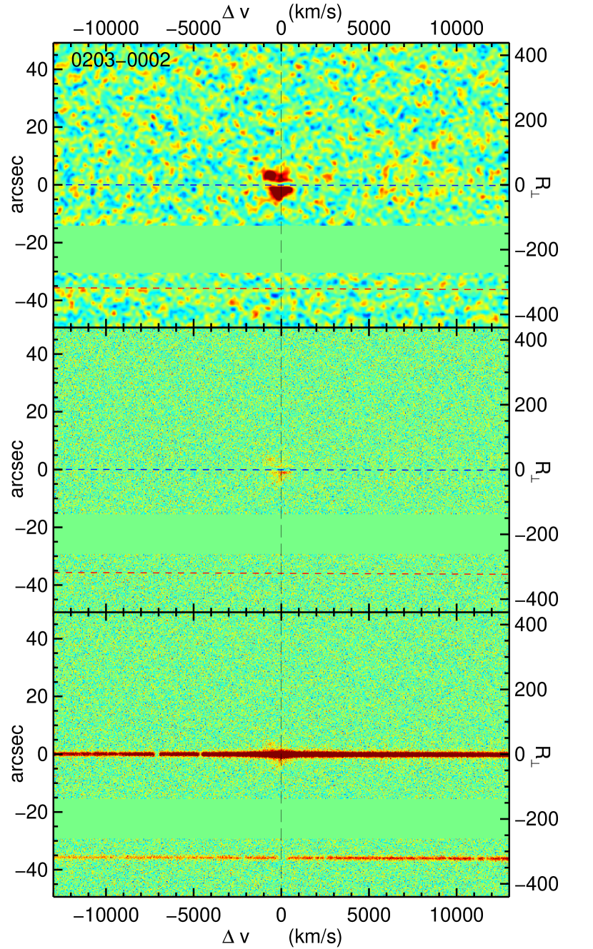
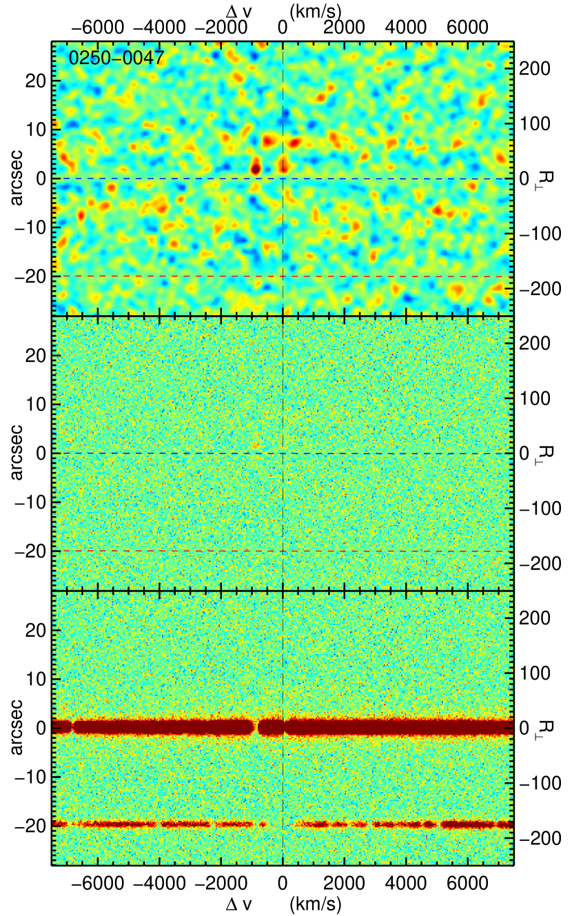
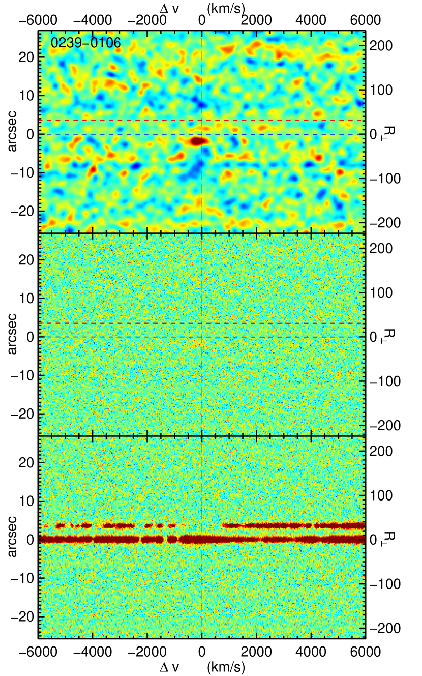
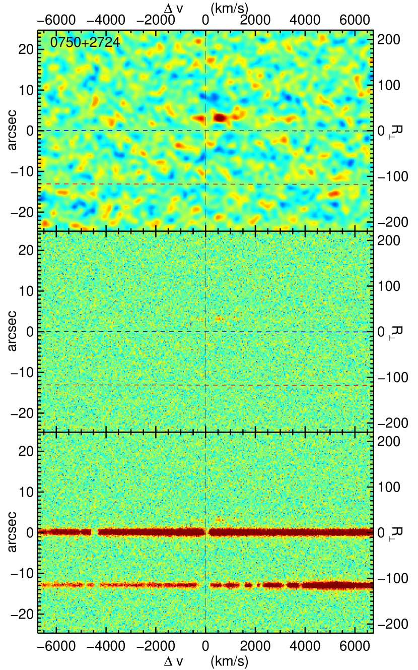
Figure 5.— Two dimensional spectra plotted as $\chi$-maps for our entire projected quasar pair sample. The bottom and middle panels show $\chi_{\rm sky}$ (sky-subtracted only) and $\chi_{\rm sky+PSF}$ (sky and PSF subtracted), respectively, as defined in §4. In the absence of extended emission, the distribution of pixel values in the the $\chi_{\rm sky+PSF}$ (middle panels) images should be Gaussian with unit variance (see Figure 3). All images are displayed with a linear stretch ranging from $-6\sigma$ to $6\sigma$ as indicated by the central color bar. Upper panels show smoothed maps $\chi_{\rm smth}$ (see §4), which are helpful for identifying extended emission. The stacked images were smoothed with a symmetric Gaussian kernel (same spatial and spectral widths) with dispersion $\sigma_{\rm smth}=100\,{\rm km~{}s}^{-1}$ (FWHM $=235\,{\rm km~{}s}^{-1}$). For LRIS this corresponds to spatially to $0.60-0.70^{\prime\prime}$, whereas for GMOS it is $0.80-0.86^{\prime\prime}$. Note that $\chi_{\rm smth}$ is the ratio of smoothed image to smoothed noise, and will hence no longer obey Gaussian statistics. Nevertheless, the same stretch and color-map are used. The horizontal red and blue dashed lines show the spectral traces for the f/g and b/g quasar, respectively, and the vertical red dotted line indicates $\Delta v=0$, corresponding to the location of the optically thick absorber coincident with the f/g quasar redshift. The name of the target is displayed at the upper left.

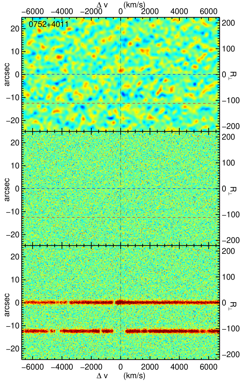
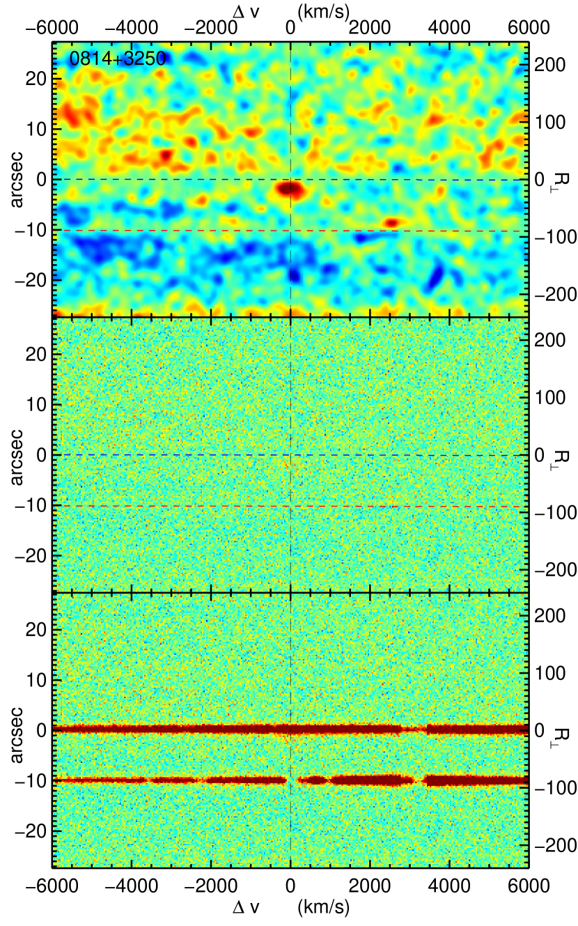
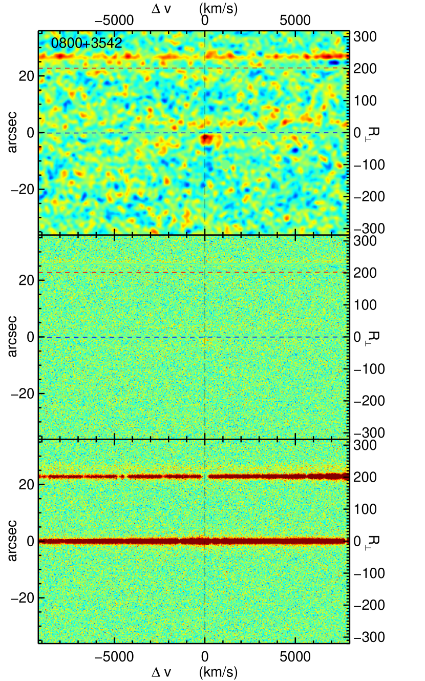
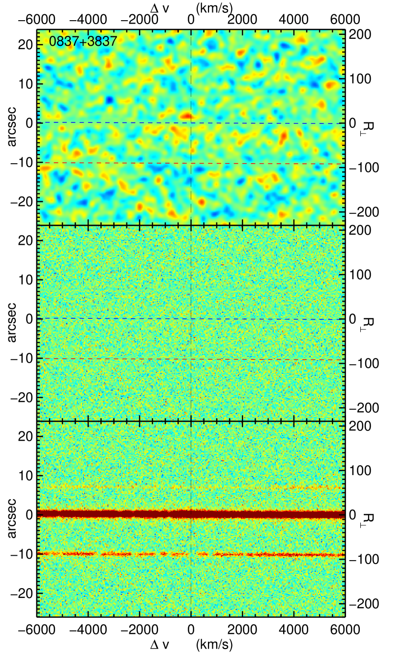
Figure 5.— Continued.

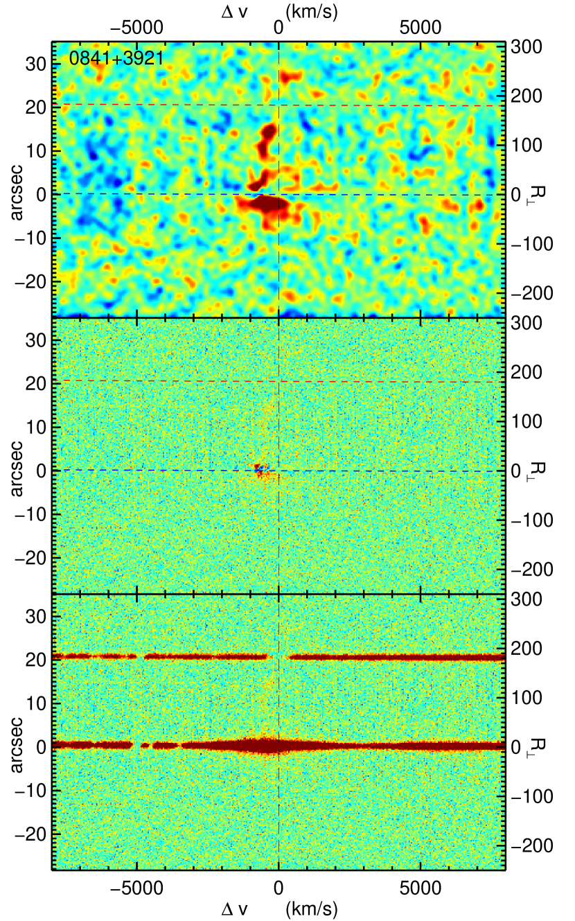
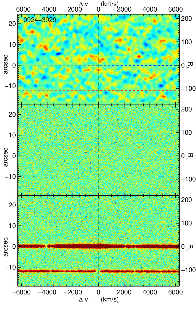
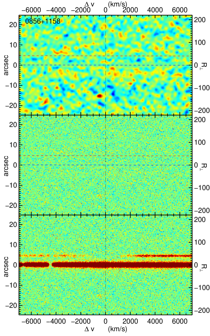
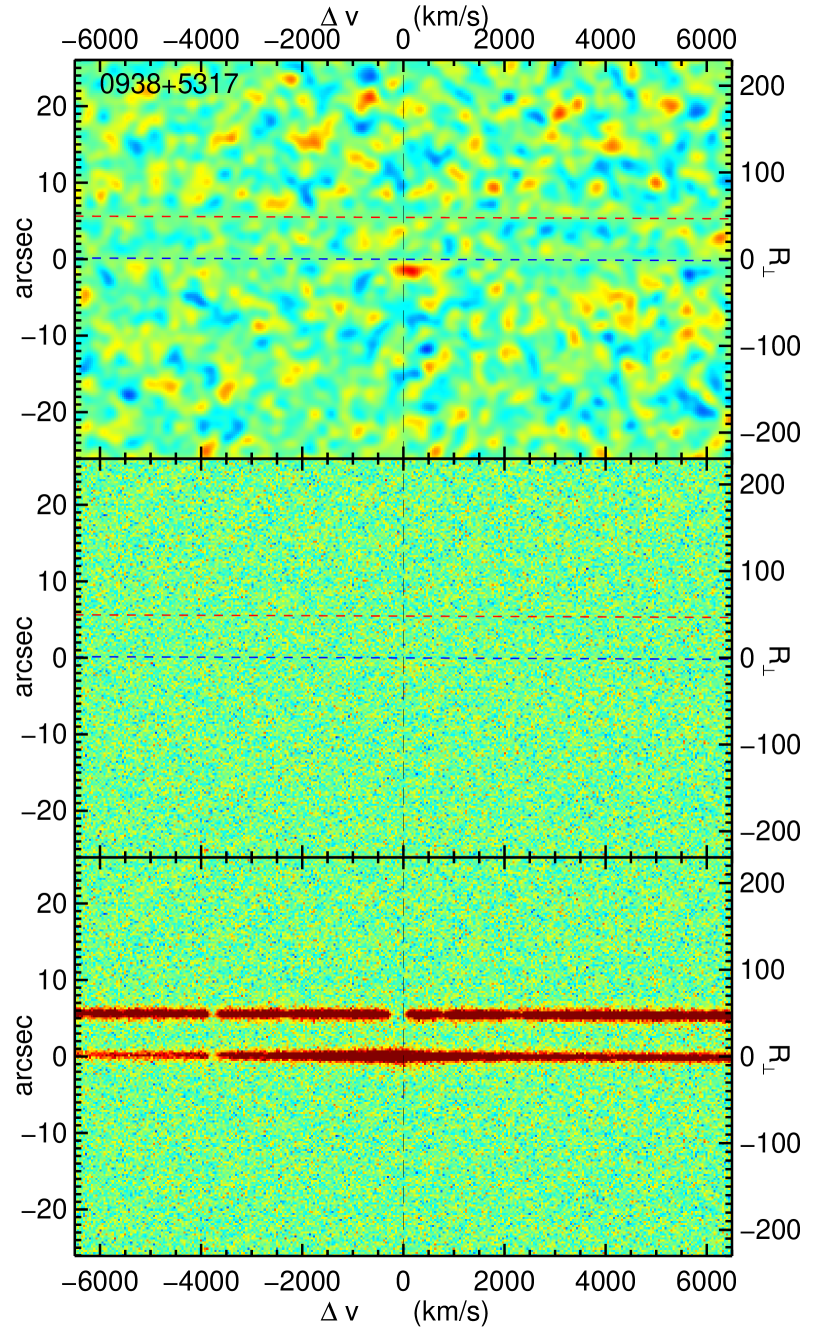
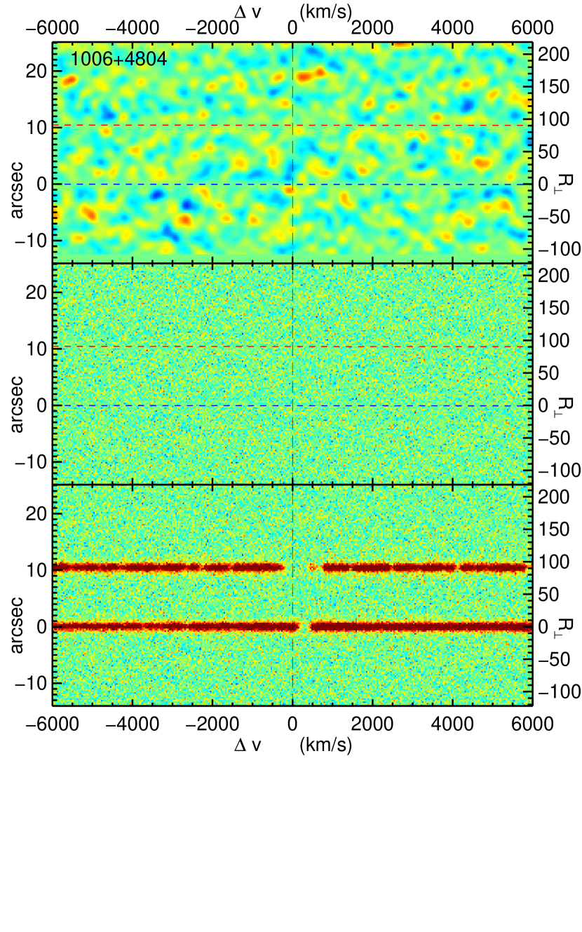
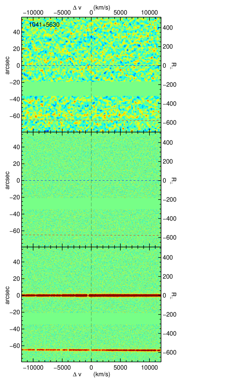
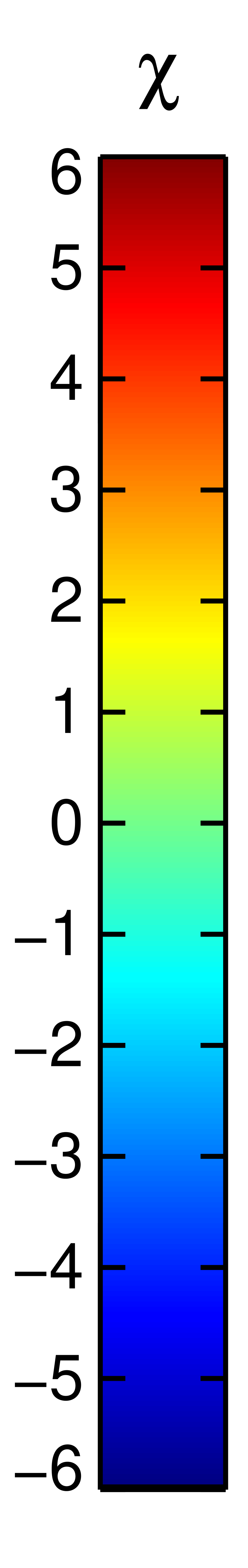
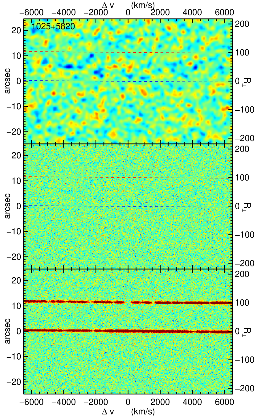
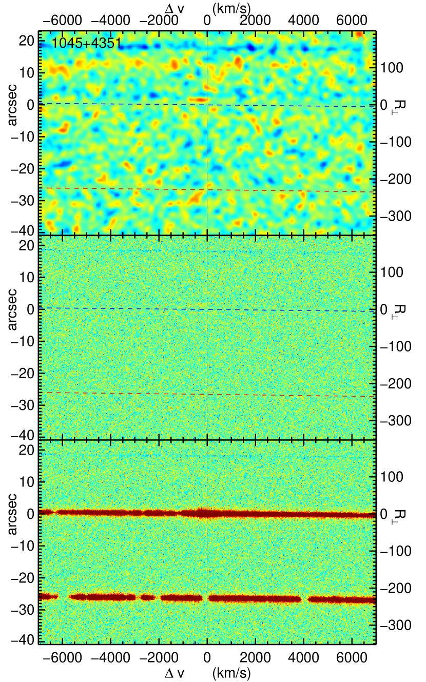
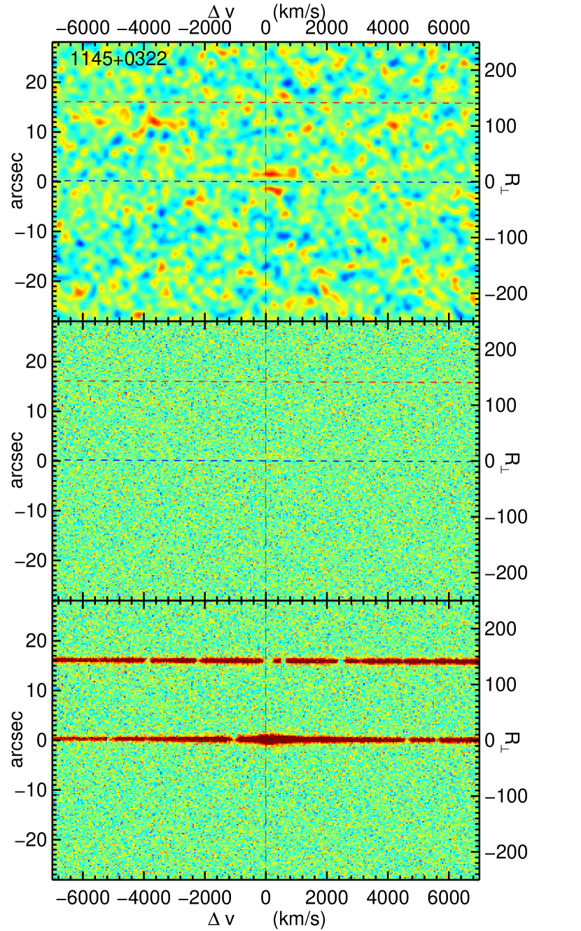
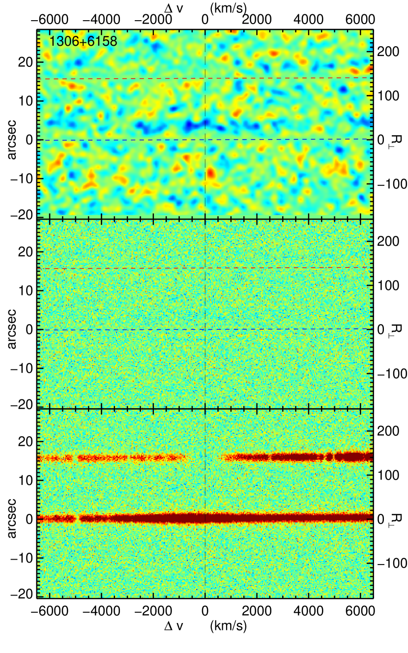
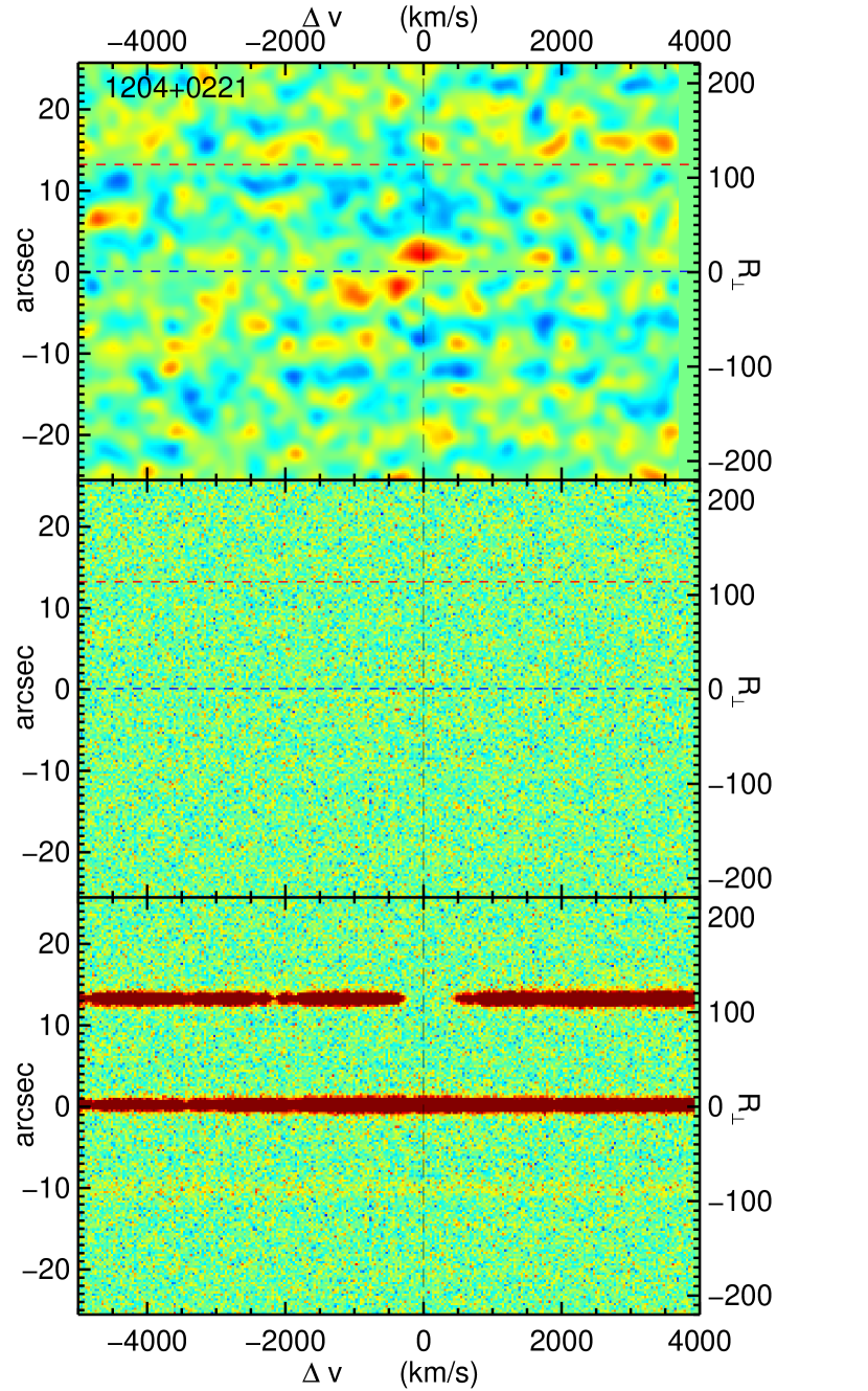
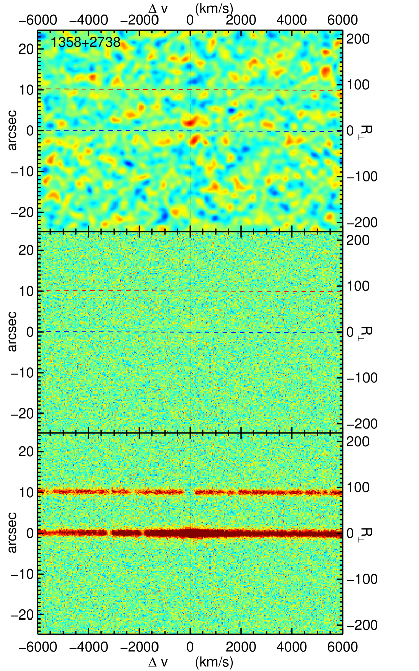
Figure 5.— Continued.

Figure 5.— Continued.

Figure 5.— Continued.

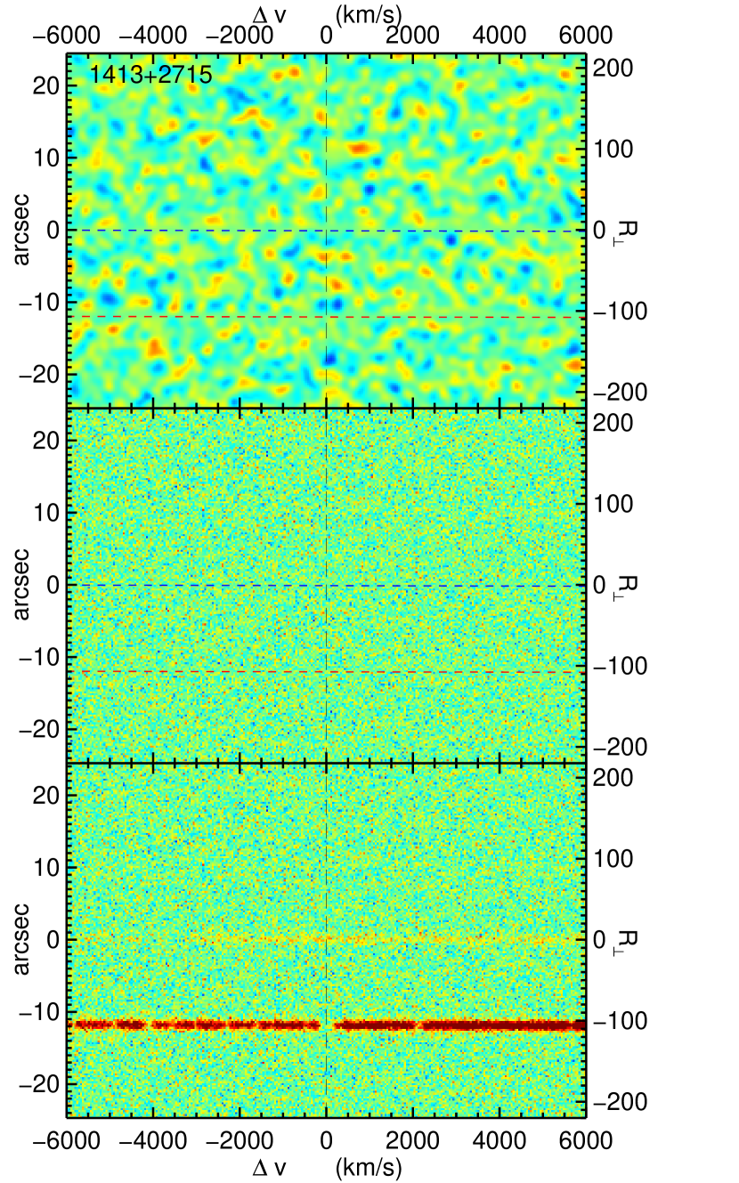
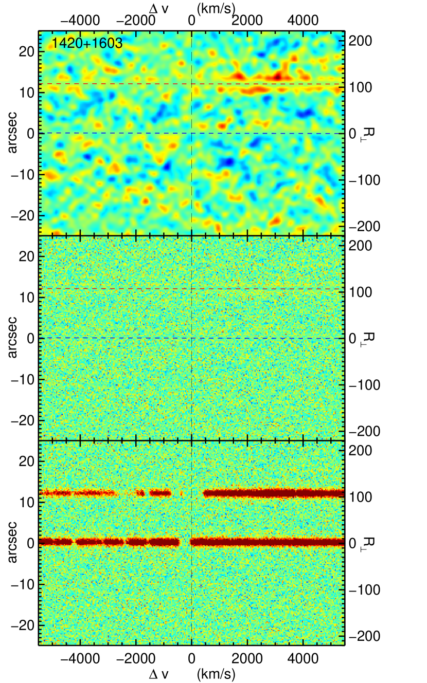
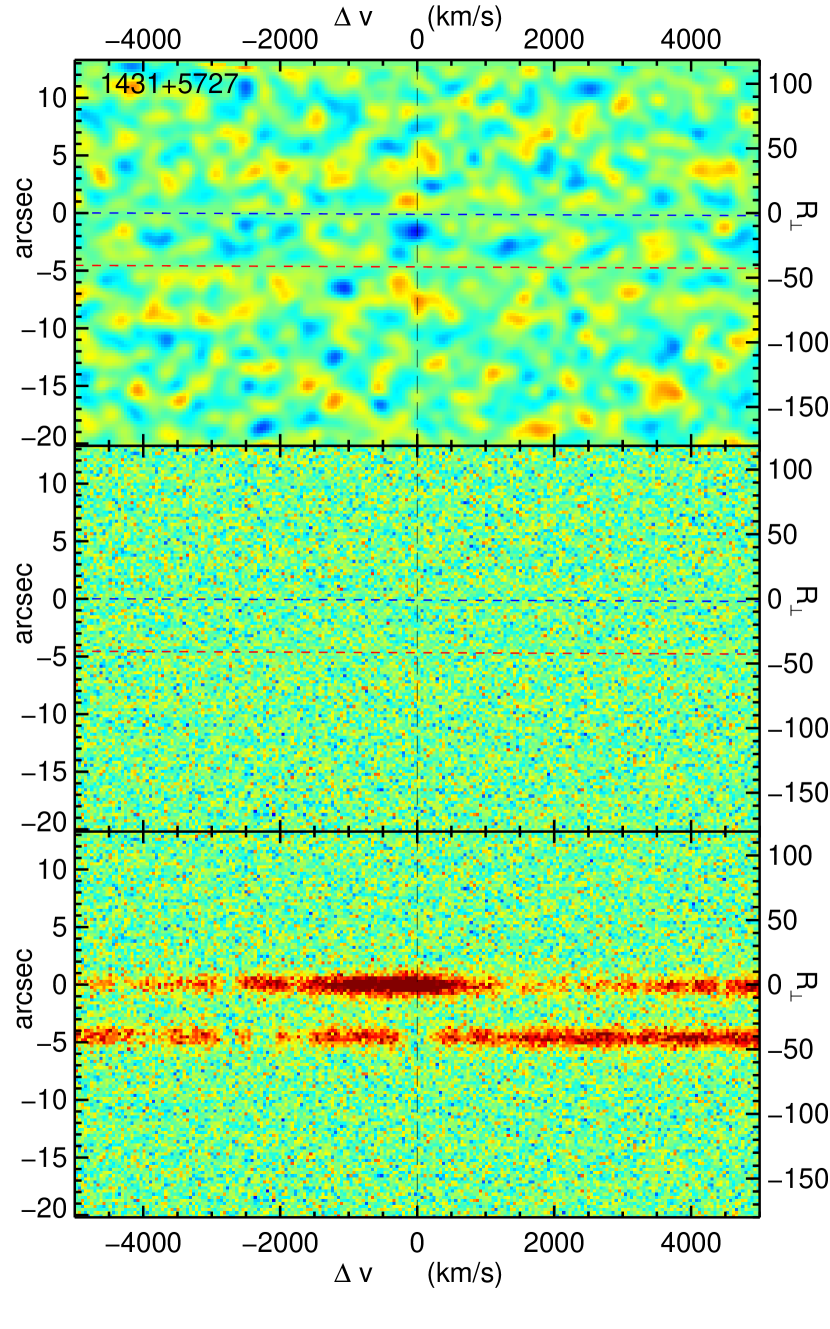
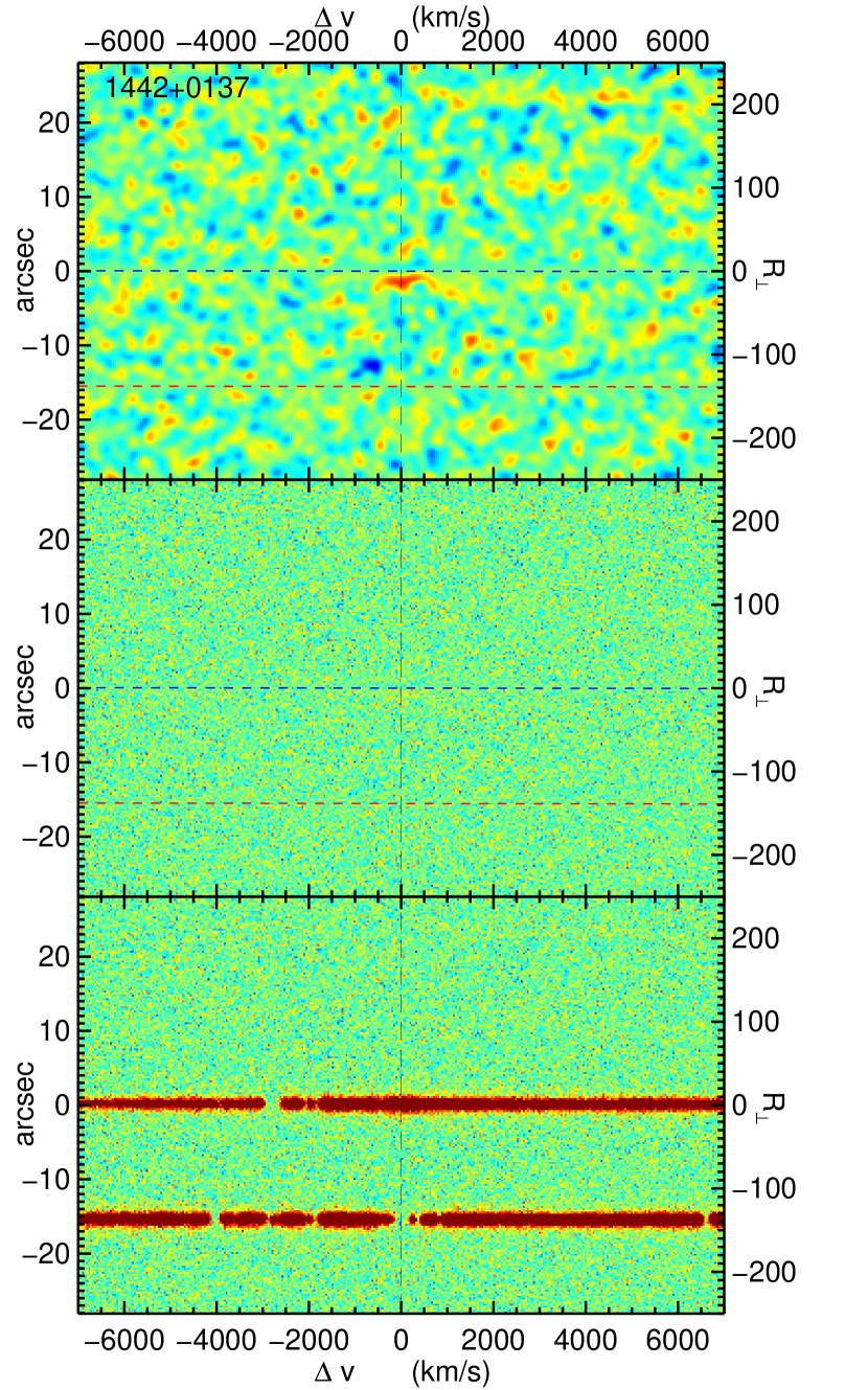
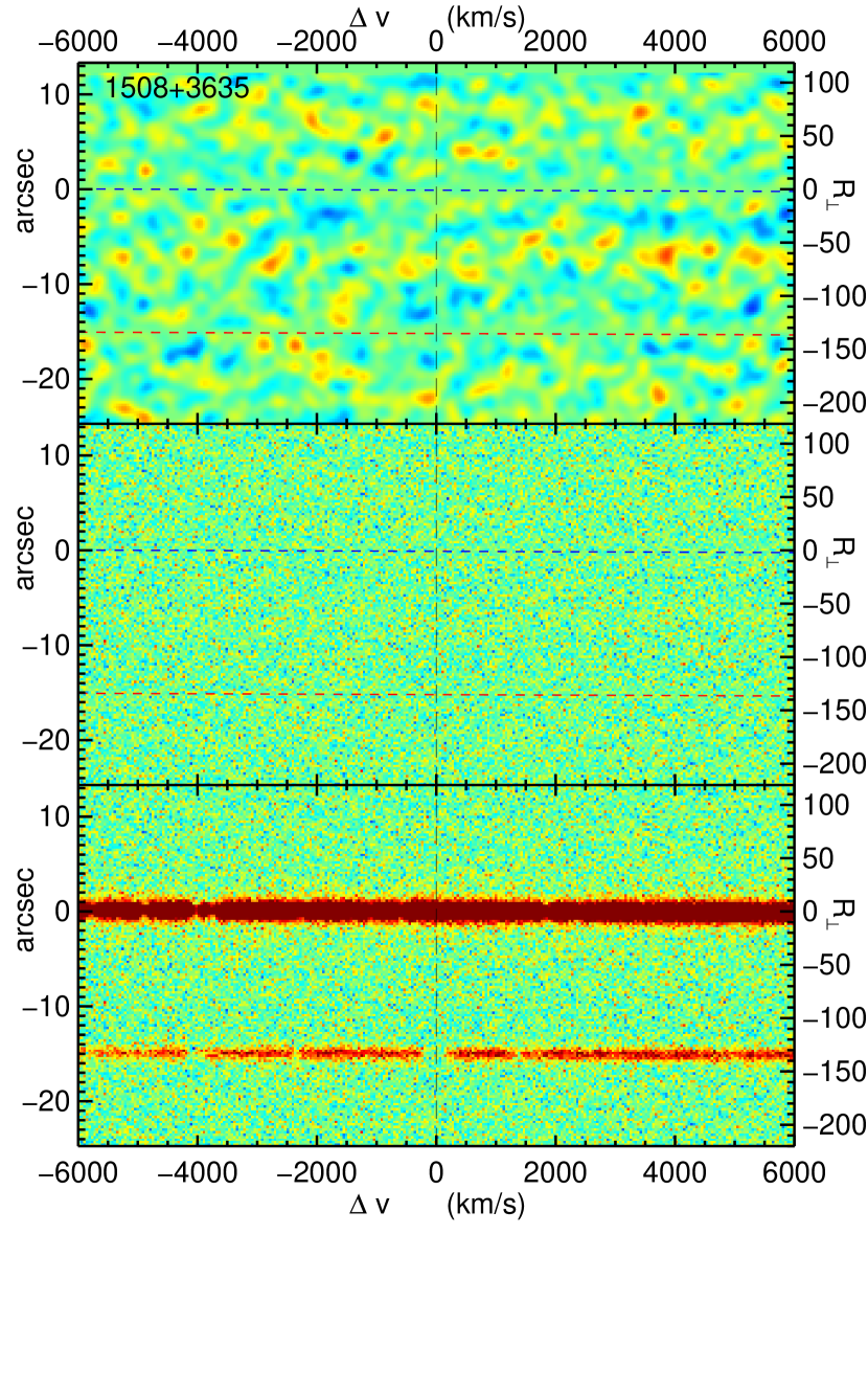
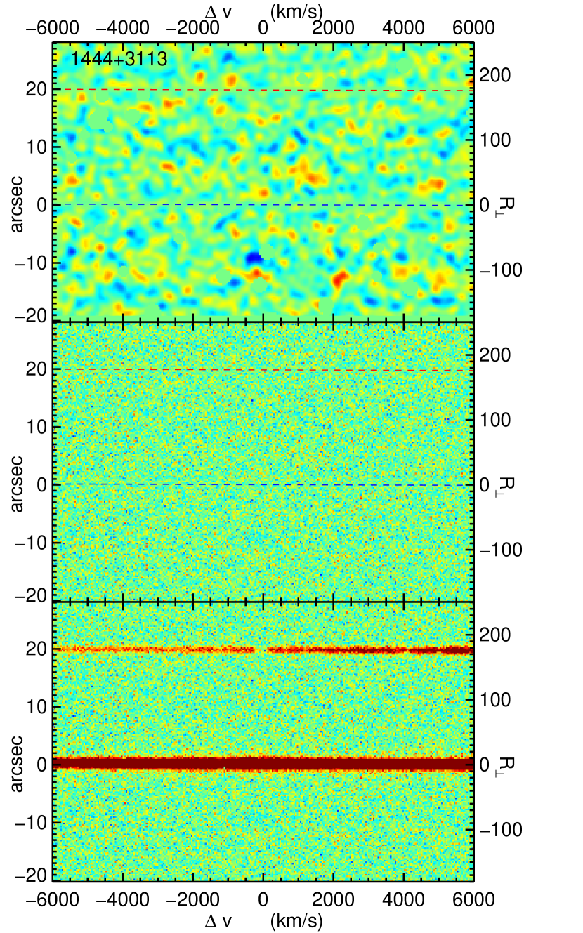
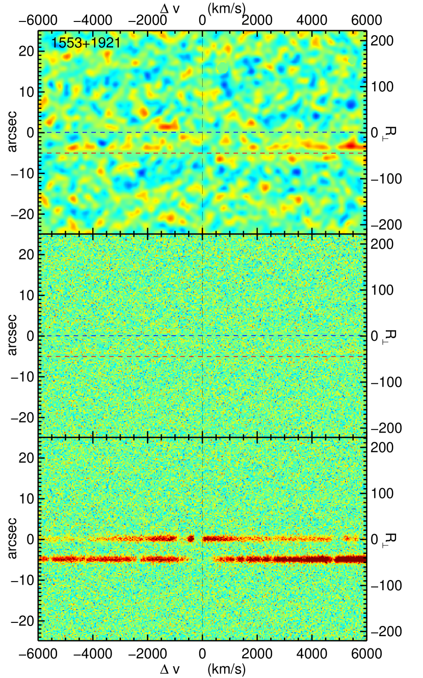
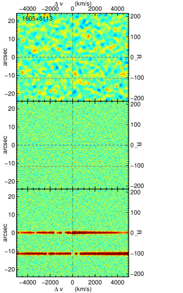
Figure 5.— Continued.

Figure 5.— Continued.

Figure 5.— Continued.

Appendix A The Attenuation of ${\rm Ly\alpha}$ by Dust

In most, if not all, astrophysical environments that contain cool gas and metals, a fraction of the refractory elements (e.g.  Fe, Ni, Si) have condensed to form dust grains. For the treatment of ${\rm Ly\alpha}$ emission considered in this paper, dust is an important factor. Because we detect absorption from gas which is optically thick in the ${\rm Ly\alpha}$ line, ${\rm Ly\alpha}$ photons will be resonantly trapped, and can only escape the system through diffusion, both in frequency and spatially. If the resonant photons must traverse a much larger pathlength to escape, this could result in a significant increase in the extinction of resonant lines compared to the continuum extinction at the same wavelength. Because the focus of this paper is ${\rm Ly\alpha}$ emission from the cold gas detected in absorption, we calculate the magnitude of the attenuation of ${\rm Ly\alpha}$ by dust grains given our expectations for the physical conditions of the gas in absorbing clouds. Our estimates closely follow the discussion in §15.7 of Draine (2011).

Consider an ionized spherical cloud with total hydrogen column density $N_{\rm H}$, neutral column density $N_{\rm HI}$, neutral fraction $x_{\rm HI}\equiv N_{\rm HI}/N_{\rm H}$, volume density $n_{\rm H}$, and Doppler broadening parameter $b$. We define the radius of the cloud to be $r_{\rm c}\equiv 3N_{\rm H}/4n_{\rm H}$, where we have used the fact that the average absorption pathlength $\langle l_{\rm c}\rangle\equiv N_{\rm H}/n_{\rm H}$ through a sphere of radius $r_{\rm c}$ equals $\langle l_{\rm c}\rangle=4/3r_{\rm c}$. In what follows we assume, that the cloud has a uniform ionization structure, whereas in reality such clouds are optically thick to ionizing photons and will be self-shielding. Uniform ionization structure is likely to be a good approximation in a cooling radiation scenario where ${\rm Ly\alpha}$ photons are generated throughout the cloud, as the bulk of the ${\rm Ly\alpha}$ photons will be generated in the regions of the cloud which have properties close to the mean. For photoionization of self-shielding clouds, this approximation is likely to over-estimate the dust attenuation, because most recombinations are generated in a thin self-shielding layer at the surface of the cloud where the neutral fraction (and hence ${\rm Ly\alpha}$ optical depth) is much lower than the average value in the cloud.

Following Draine (2011), we can write the mean square displacement of a ${\rm Ly\alpha}$ photon from the point of emission as

$$\langle r^{2}\rangle\approx\frac{2}{3}L_{0}^{2}N_{\rm s}^{3}$$ (A1)

where

$$L_{0}\equiv\frac{1}{n_{\rm HI}\sigma_{w}},$$ (A2)

$$\sigma_{w}=6.48{\;\times\;10^{-18}}\,{\rm cm}^{-2}\left(\frac{b}{20\,{\rm km~{}s}^{-1}}\right)^{-2}$$ (A3)

and $N_{\rm s}$ is the total number of resonant scatterings and $\sigma_{w}$ is the H I absorption cross-section. These expressions are valid in the Lorentzian wings of the Voigt profile where the bulk of the spatial diffusion takes place. A reasonable criterion for escape is that $\langle r^{2}\rangle=r_{\rm c}^{2}$, from which we can determine the total number of scatterings via eqn. (A1)

$$N_{\rm s}\approx 15\left(\frac{N_{\rm HI}}{10^{19}\,{\rm cm}^{-2}}\right)^{2/3}\left(\frac{b}{20\,{\rm km~{}s}^{-1}}\right)^{-4/3}.$$ (A4)

This modest number of scatterings is sufficient to frequency-shift a typical photon to $\Delta\nu/\nu\approx N_{\rm s}^{1/2}b/c$, such that our assumption of being in the damping wings of the Voigt profile is valid.

To determine the amount of attenuation by dust, we must first estimate the total pathlength traveled by an escaping photon, which can be written as $s\approx 1/2L_{0}N_{\rm s}^{2}$ (Draine 2011), or

$$s\approx 1.8\left(\frac{N_{\rm HI}}{10^{19}\,{\rm cm}^{-2}}\right)^{1/3}\left(\frac{b}{20\,{\rm km~{}s}^{-1}}\right)^{-2/3}\langle l_{\rm c}\rangle.$$ (A5)

Thus given the cloud properties we have assumed, the pathlength and hence total optical depth through the cloud for resonantly scattered photons is a factor of $\sim 2$ larger than it is for continuum photons.

The amount of extinction corresponding to this pathlength depends on the amount of dust associated with the gas, which is highly uncertain. In quasar absorption line research, there is strong evidence that refractory elements in DLAs are depleted onto dust grains albeit at modest levels compared to the Galactic ISM (Pettini et al. 1994; Prochaska & Wolfe 2001; Vladilo et al. 2011). The effects appear to be strongest for the systems with highest metallicity (e.g. Kaplan et al. 2010). For LLSs where the gas is predominantly ionized, there has been essentially no empirical assessment of dust. One expects that the physical conditions – higher UV radiation field, higher temperature, lower density – lead to lower dust-to-gas ratios. Nevertheless, dust is apparent in highly ionized regions of the local universe (e.g. Draine 2011) and also the diffuse environment of galactic halos (Ménard et al. 2010). The most extreme assumption is to assume that all of the gas contains dust, and that the dust-to-gas ratio corresponds to that of the Milky Way, which is equivalent to assuming a solar metallicity and a high depletion factor. This is conservative, because DLAs are observed to have lower depletions than the Milky Way ISM and it is rather unlikely that all of gas in the CGM of quasars has solar enrichment as we assume. For example, our detailed analysis of SDSSJ1204+0221 in (Prochaska & Hennawi 2009) showed metallicities in the range $0.3-1.6\,Z_{\odot}$, and our expectation is that a more typical metallicity of the quasar CGM $\sim 0.1\,Z_{\odot}$ (Prochaska et al. 2012, Prochaska et al., in prep.).

The continuum extinction at $\lambda=1216$Å can be written $A^{\rm cont}_{\rm 1216}=0.18(R_{\rm V}/3.1)(N_{\rm H}/10^{20}\,{\rm cm^{-2}})\,{\rm mag}$, corresponding to a visual extinction of $A_{\rm V}=0.05$, where we take $A^{\rm cont}_{\rm 1216}/A_{\rm V}=3.3$ based on the extinction curves of (Fitzpatrick 1999) for $R_{\rm V}=3.1$. In the absence of resonant effects, 1216Å photons would be attenuated according to the continuum extinction $A^{\rm cont}_{\rm 1216}$. Combining this extinction with the increased resonant pathelngth in eqn. (A5), we can write the total resonant extinction that ${\rm Ly\alpha}$ photons suffer as they ecape the cloud as

$$A^{\rm res}_{\rm 1216}=0.32\left(\frac{x_{\rm HI}}{0.1}\right)\!\left(\frac{N_{\rm HI}}{10^{19}\,{\rm cm}^{-2}}\right)^{4/3}\!\left(\frac{b}{20\,{\rm km~{}s}^{-1}}\right)^{-2/3}.$$ (A6)

Once ${\rm Ly\alpha}$ photons escape an individual cloud, they propagate freely until they encounter other clouds, where they might undergo additional resonant scattering. But the probability of this occurring is small, since it requires both spatial and spectral overlap. If the spatial covering factor of clouds is $f_{\rm C}$, and if bulk motions of the clouds in the quasar halo follow a gaussian with line-of-sight dispersion $\sigma$, then the probability of additional resonant scattering is $\sim f_{\rm C}N_{\rm s}^{1/2}b/\sqrt{2}\sigma\sim 0.07$ for typical numbers ($N_{\rm s}=15$, $f_{\rm C}=0.50$, $\sigma=400{\rm km~{}s}^{-1}$, and $b=20{\rm km~{}s}^{-1}$), thus additional scattering would amount to $\lesssim 10\%$ corrections to the total extinction, which is already highly uncertain because of the unknown dust-to-gas ratio. However, in traversing additional material ${\rm Ly\alpha}$ photons will still encounter continuum extinction, so we can heuristically write the total extinction as $A_{1216}\approx A^{\rm res}_{1216}+f_{\rm C}A^{\rm cont}_{\rm 1216}$.

Thus given the observed properties of the quasar CGM ($N_{\rm HI}\sim 10^{19}\,{\rm cm}^{-2}$; $x_{\rm HI}\sim 0.1$; $b\sim 20\,{\rm km~{}s}^{-1}$), and under the most conservative assumptions regarding the amount of dust, namely a Milky Way dust-to-gas ratio (corresponding to solar metallicity and high depletion), we conclude that the extinction of ${\rm Ly\alpha}$ photons would be in the range of $A_{1216}\approx 0.3-0.6$, resulting in at most a factor of $\sim 2$ reduction in the total ${\rm Ly\alpha}$ surface brightness. This extinction scales linearly with the metallicity, and as mentioned previously, it is unlikely that all gas in the quasar CGM has solar enrichment as we have assumed. Furthermore, our estimate of the extinction due to resonance effects is appropriate for ${\rm Ly\alpha}$ photons generated throughout the volume of an emitting cloud, as expected in a cooling radiation scenario, whereas it is likely overestimates the attenuation of flourescent emission powered by photoionization.

Finally, it is worth asking whether the continuum extinction from CGM absorbers would be detectable via the reddening of the b/g quasar spectra. Consider for example the absorber in SDSSJ1204+0221  which we analayzed in detail in (Prochaska & Hennawi 2009). Our photoionization modeling gave a higher total gas column density of $N_{\rm H}=10^{20.5}\,{\rm cm^{-2}}$, which implies a continuum extinction of $A^{\rm cont}_{\rm 1216}=0.57$, for solar metallicity and a Milky Way dust to gas ratio. This reddening would not be distinguishable from either the SDSS photometry or our optical spectra, since the relative reddening $A^{\rm cont}_{\rm 1216}-A^{\rm cont}_{\rm 2500}=0.18$ between rest frame wavelengths $\lambda=1216$Å and 2500Å (corresponding to the observed frame $4000-8000$Å covered by the optical spectra and photometry) is small, and cannot be distinguished from intrinsic variations in the quasar continuum slopes.

References

- Abazajian et al. (2005) Abazajian, K., Adelman-McCarthy, J. K., Agüeros, M. A., Allam, S. S., Anderson, K. S. J., Anderson, S. F., Annis, J., Bahcall, N. A., Baldry, I. K., Bastian, S., Berlind, A., Bernardi, M., Blanton, M. R., Bochanski, Jr., J. J., Boroski, W. N., Brewington, H. J., Briggs, J. W., Brinkmann, J., Brunner, R. J., Budavári, T., Carey, L. N., Castander, F. J., Connolly, A. J., Covey, K. R., Csabai, I., Dalcanton, J. J., Doi, M., Dong, F., Eisenstein, D. J., Evans, M. L., Fan, X., Finkbeiner, D. P., Friedman, S. D., Frieman, J. A., Fukugita, M., Gillespie, B., Glazebrook, K., Gray, J., Grebel, E. K., Gunn, J. E., Gurbani, V. K., Hall, P. B., Hamabe, M., Harbeck, D., Harris, F. H., Harris, H. C., Harvanek, M., Hawley, S. L., Hayes, J., Heckman, T. M., Hendry, J. S., Hennessy, G. S., Hindsley, R. B., Hogan, C. J., Hogg, D. W., Holmgren, D. J., Holtzman, J. A., Ichikawa, S.-i., Ichikawa, T., Ivezić, Ž., Jester, S., Johnston, D. E., Jorgensen, A. M., Jurić, M., Kent, S. M., Kleinman, S. J., Knapp, G. R., Kniazev, A. Y., Kron, R. G., Krzesinski, J., Lamb, D. Q., Lampeitl, H., Lee, B. C., Lin, H., Long, D. C., Loveday, J., Lupton, R. H., Mannery, E., Margon, B., Martínez-Delgado, D., Matsubara, T., McGehee, P. M., McKay, T. A., Meiksin, A., Ménard, B., Munn, J. A., Nash, T., Neilsen, Jr., E. H., Newberg, H. J., Newman, P. R., Nichol, R. C., Nicinski, T., Nieto-Santisteban, M., Nitta, A., Okamura, S., O’Mullane, W., Owen, R., Padmanabhan, N., Pauls, G., Peoples, J., Pier, J. R., Pope, A. C., Pourbaix, D., Quinn, T. R., Raddick, M. J., Richards, G. T., Richmond, M. W., Rix, H.-W., Rockosi, C. M., Schlegel, D. J., Schneider, D. P., Schroeder, J., Scranton, R., Sekiguchi, M., Sheldon, E., Shimasaku, K., Silvestri, N. M., Smith, J. A., Smolčić, V., Snedden, S. A., Stebbins, A., Stoughton, C., Strauss, M. A., SubbaRao, M., Szalay, A. S., Szapudi, I., Szkody, P., Szokoly, G. P., Tegmark, M., Teodoro, L., Thakar, A. R., Tremonti, C., Tucker, D. L., Uomoto, A., Vanden Berk, D. E., Vandenberg, J., Vogeley, M. S., Voges, W., Vogt, N. P., Walkowicz, L. M., Wang, S.-i., Weinberg, D. H., West, A. A., White, S. D. M., Wilhite, B. C., Xu, Y., Yanny, B., Yasuda, N., Yip, C.-W., Yocum, D. R., York, D. G., Zehavi, I., Zibetti, S., & Zucker, D. B. 2005, AJ, 129, 1755
- Adelberger & Steidel (2005) Adelberger, K. L., & Steidel, C. C. 2005, ApJ, 627, L1
- Adelberger et al. (2006) Adelberger, K. L., Steidel, C. C., Kollmeier, J. A., & Reddy, N. A. 2006, ApJ, 637, 74
- Ahn et al. (2012) Ahn, C. P., Alexandroff, R., Allende Prieto, C., Anderson, S. F., Anderton, T., Andrews, B. H., Aubourg, É., Bailey, S., Balbinot, E., Barnes, R., & et al. 2012, ApJS, 203, 21
- Alam & Miralda-Escudé (2002) Alam, S. M. K., & Miralda-Escudé, J. 2002, ApJ, 568, 576
- Antonucci (1993) Antonucci, R. 1993, ARA&A, 31, 473
- Bacon et al. (2010) Bacon, R., Accardo, M., Adjali, L., Anwand, H., Bauer, S., Biswas, I., Blaizot, J., Boudon, D., Brau-Nogue, S., Brinchmann, J., Caillier, P., Capoani, L., Carollo, C. M., Contini, T., Couderc, P., Daguisé, E., Deiries, S., Delabre, B., Dreizler, S., Dubois, J., Dupieux, M., Dupuy, C., Emsellem, E., Fechner, T., Fleischmann, A., François, M., Gallou, G., Gharsa, T., Glindemann, A., Gojak, D., Guiderdoni, B., Hansali, G., Hahn, T., Jarno, A., Kelz, A., Koehler, C., Kosmalski, J., Laurent, F., Le Floch, M., Lilly, S. J., Lizon, J.-L., Loupias, M., Manescau, A., Monstein, C., Nicklas, H., Olaya, J.-C., Pares, L., Pasquini, L., Pécontal-Rousset, A., Pelló, R., Petit, C., Popow, E., Reiss, R., Remillieux, A., Renault, E., Roth, M., Rupprecht, G., Serre, D., Schaye, J., Soucail, G., Steinmetz, M., Streicher, O., Stuik, R., Valentin, H., Vernet, J., Weilbacher, P., Wisotzki, L., & Yerle, N. 2010, in Society of Photo-Optical Instrumentation Engineers (SPIE) Conference Series, Vol. 7735, Society of Photo-Optical Instrumentation Engineers (SPIE) Conference Series
- Barnes & Haehnelt (2009) Barnes, L. A., & Haehnelt, M. G. 2009, MNRAS, 397, 511
- Barnes & Haehnelt (2010) —. 2010, MNRAS, 403, 870
- Barnes et al. (2011) Barnes, L. A., Haehnelt, M. G., Tescari, E., & Viel, M. 2011, MNRAS, 416, 1723
- Barrio et al. (2008) Barrio, F. E., Jarvis, M. J., Rawlings, S., Bauer, A., Croft, S., Hill, G. J., Manchado, A., McLure, R. J., Smith, D. J. B., & Targett, T. A. 2008, MNRAS, 389, 792
- Basu-Zych & Scharf (2004) Basu-Zych, A., & Scharf, C. 2004, ApJ, 615, L85
- Becker et al. (1995) Becker, R. H., White, R. L., & Helfand, D. J. 1995, ApJ, 450, 559
- Bertone & Schaye (2010) Bertone, S., & Schaye, J. 2010, ArXiv e-prints
- Binette et al. (1993) Binette, L., Wang, J. C. L., Zuo, L., & Magris, C. G. 1993, AJ, 105, 797
- Binette et al. (2006) Binette, L., Wilman, R. J., Villar-Martín, M., Fosbury, R. A. E., Jarvis, M. J., & Röttgering, H. J. A. 2006, A&A, 459, 31
- Birnboim et al. (2007) Birnboim, Y., Dekel, A., & Neistein, E. 2007, MNRAS, 380, 339
- Bolton et al. (2005) Bolton, J. S., Haehnelt, M. G., Viel, M., & Springel, V. 2005, MNRAS, 357, 1178
- Bovy et al. (2011) Bovy, J., Hennawi, J. F., Hogg, D. W., Myers, A. D., Kirkpatrick, J. A., Schlegel, D. J., Ross, N. P., Sheldon, E. S., McGreer, I. D., Schneider, D. P., & Weaver, B. A. 2011, ApJ, 729, 141
- Bovy et al. (2012) Bovy, J., Myers, A. D., Hennawi, J. F., Hogg, D. W., McMahon, R. G., Schiminovich, D., Sheldon, E. S., Brinkmann, J., Schneider, D. P., & Weaver, B. A. 2012, ApJ, 749, 41
- Bowen et al. (2006) Bowen, D. V., Hennawi, J. F., Ménard, B., Chelouche, D., Inada, N., Oguri, M., Richards, G. T., Strauss, M. A., Vanden Berk, D. E., & York, D. G. 2006, ApJ, 645, L105
- Bremer et al. (1992) Bremer, M. N., Fabian, A. C., Sargent, W. L. W., Steidel, C. C., Boksenberg, A., & Johnstone, R. M. 1992, MNRAS, 258, 23P
- Brooks et al. (2009) Brooks, A. M., Governato, F., Quinn, T., Brook, C. B., & Wadsley, J. 2009, ApJ, 694, 396
- Bunker et al. (2003) Bunker, A., Smith, J., Spinrad, H., Stern, D., & Warren, S. 2003, Ap&SS, 284, 357
- Bunker et al. (1998) Bunker, A. J., Marleau, F. R., & Graham, J. R. 1998, AJ, 116, 2086
- Bunker et al. (1999) —. 1999, ArXiv Astrophysics e-prints
- Cantalupo et al. (2012) Cantalupo, S., Lilly, S. J., & Haehnelt, M. G. 2012, ArXiv e-prints
- Cantalupo et al. (2007) Cantalupo, S., Lilly, S. J., & Porciani, C. 2007, ApJ, 657, 135
- Cantalupo et al. (2005) Cantalupo, S., Porciani, C., Lilly, S. J., & Miniati, F. 2005, ApJ, 628, 61
- Chamberlain (1953) Chamberlain, J. W. 1953, ApJ, 117, 387
- Chapman et al. (2004) Chapman, S. C., Scott, D., Windhorst, R. A., Frayer, D. T., Borys, C., Lewis, G. F., & Ivison, R. J. 2004, ApJ, 606, 85
- Chelouche et al. (2007) Chelouche, D., Ménard, B., Bowen, D. V., & Gnat, O. 2007, ArXiv e-prints, 706
- Christensen et al. (2006) Christensen, L., Jahnke, K., Wisotzki, L., & Sánchez, S. F. 2006, A&A, 459, 717
- Ciardullo et al. (2012) Ciardullo, R., Gronwall, C., Wolf, C., McCathran, E., Bond, N. A., Gawiser, E., Guaita, L., Feldmeier, J. J., Treister, E., Padilla, N., Francke, H., Matković, A., Altmann, M., & Herrera, D. 2012, ApJ, 744, 110
- Colbert et al. (2006) Colbert, J. W., Teplitz, H., Francis, P., Palunas, P., Williger, G. M., & Woodgate, B. 2006, ApJ, 637, L89
- Courbin et al. (2008) Courbin, F., North, P., Eigenbrod, A., & Chelouche, D. 2008, ArXiv e-prints, 803
- Crotts (1989) Crotts, A. P. S. 1989, ApJ, 336, 550
- Dayal et al. (2010) Dayal, P., Ferrara, A., & Saro, A. 2010, MNRAS, 402, 1449
- De Breuck et al. (2004) De Breuck, C., Bertoldi, F., Carilli, C., Omont, A., Venemans, B., Röttgering, H., Overzier, R., Reuland, M., Miley, G., Ivison, R., & van Breugel, W. 2004, A&A, 424, 1
- Dekel & Birnboim (2006) Dekel, A., & Birnboim, Y. 2006, MNRAS, 368, 2
- Dekel et al. (2009) Dekel, A., Birnboim, Y., Engel, G., Freundlich, J., Goerdt, T., Mumcuoglu, M., Neistein, E., Pichon, C., Teyssier, R., & Zinger, E. 2009, Nature, 457, 451
- Dey et al. (2005) Dey, A., Bian, C., Soifer, B. T., Brand, K., Brown, M. J. I., Chaffee, F. H., Le Floc’h, E., Hill, G., Houck, J. R., Jannuzi, B. T., Rieke, M., Weedman, D., Brodwin, M., & Eisenhardt, P. 2005, ApJ, 629, 654
- Dijkstra et al. (2006a) Dijkstra, M., Haiman, Z., & Spaans, M. 2006a, ApJ, 649, 14
- Dijkstra et al. (2006b) —. 2006b, ApJ, 649, 14
- Dijkstra et al. (2006c) —. 2006c, ApJ, 649, 37
- Dijkstra & Kramer (2012) Dijkstra, M., & Kramer, R. 2012, MNRAS, 424, 1672
- Dijkstra & Loeb (2009) Dijkstra, M., & Loeb, A. 2009, MNRAS, 400, 1109
- Djorgovski et al. (1985) Djorgovski, S., Spinrad, H., McCarthy, P., & Strauss, M. A. 1985, ApJ, 299, L1
- D’Odorico et al. (2008) D’Odorico, V., Bruscoli, M., Saitta, F., Fontanot, F., Viel, M., Cristiani, S., & Monaco, P. 2008, MNRAS, 389, 1727
- Draine (2011) Draine, B. T. 2011, Physics of the Interstellar and Intergalactic Medium
- Elvis (2000) Elvis, M. 2000, ApJ, 545, 63
- Fardal et al. (2001) Fardal, M. A., Katz, N., Gardner, J. P., Hernquist, L., Weinberg, D. H., & Davé, R. 2001, ApJ, 562, 605
- Farina et al. (2012) Farina, E. P., Falomo, R., Decarli, R., Treves, A., & Kotilainen, J. K. 2012, MNRAS, 369
- Faucher-Giguère et al. (2010) Faucher-Giguère, C.-A., Kereš, D., Dijkstra, M., Hernquist, L., & Zaldarriaga, M. 2010, ApJ, 725, 633
- Faucher-Giguère et al. (2008) Faucher-Giguère, C.-A., Lidz, A., Hernquist, L., & Zaldarriaga, M. 2008, ApJ, 688, 85
- Fitzpatrick (1999) Fitzpatrick, E. L. 1999, PASP, 111, 63
- Francis & Bland-Hawthorn (2004) Francis, P. J., & Bland-Hawthorn, J. 2004, MNRAS, 353, 301
- Francis & McDonnell (2006) Francis, P. J., & McDonnell, S. 2006, MNRAS, 370, 1372
- Francis et al. (2001) Francis, P. J., Williger, G. M., Collins, N. R., Palunas, P., Malumuth, E. M., Woodgate, B. E., Teplitz, H. I., Smette, A., Sutherland, R. S., Danks, A. C., Hill, R. S., Lindler, D., Kimble, R. A., Heap, S. R., & Hutchings, J. B. 2001, ApJ, 554, 1001
- Frank et al. (2012) Frank, S., Rasera, Y., Vibert, D., Milliard, B., Popping, A., Blaizot, J., Courty, S., Deharveng, J.-M., Péroux, C., Teyssier, R., & Martin, C. D. 2012, MNRAS, 420, 1731
- Fu & Stockton (2006) Fu, H., & Stockton, A. 2006, ApJ, 650, 80
- Fu & Stockton (2007) —. 2007, ApJ, 666, 794
- Fu & Stockton (2009) —. 2009, ApJ, 690, 953
- Furlanetto et al. (2005) Furlanetto, S. R., Schaye, J., Springel, V., & Hernquist, L. 2005, ApJ, 622, 7
- Fynbo et al. (2001) Fynbo, J. U., Möller, P., & Thomsen, B. 2001, A&A, 374, 443
- Fynbo et al. (1999) Fynbo, J. U., Møller, P., & Warren, S. J. 1999, MNRAS, 305, 849
- Gaskell (1982) Gaskell, C. M. 1982, ApJ, 263, 79
- Geach et al. (2007) Geach, J. E., Smail, I., Chapman, S. C., Alexander, D. M., Blain, A. W., Stott, J. P., & Ivison, R. J. 2007, ApJ, 655, L9
- Gilli et al. (2007) Gilli, R., Comastri, A., & Hasinger, G. 2007, A&A, 463, 79
- Goerdt et al. (2010) Goerdt, T., Dekel, A., Sternberg, A., Ceverino, D., Teyssier, R., & Primack, J. R. 2010, MNRAS, 933
- Gould & Weinberg (1996) Gould, A., & Weinberg, D. H. 1996, ApJ, 468, 462
- Greene et al. (2011) Greene, J. E., Zakamska, N. L., Ho, L. C., & Barth, A. J. 2011, ApJ, 732, 9
- Guaita et al. (2011) Guaita, L., Acquaviva, V., Padilla, N., Gawiser, E., Bond, N. A., Ciardullo, R., Treister, E., Kurczynski, P., Gronwall, C., Lira, P., & Schawinski, K. 2011, ApJ, 733, 114
- Haiman & Rees (2001) Haiman, Z., & Rees, M. J. 2001, ApJ, 556, 87
- Haiman et al. (2000) Haiman, Z., Spaans, M., & Quataert, E. 2000, ApJ, 537, L5
- Heckman et al. (1991a) Heckman, T. M., Lehnert, M. D., Miley, G. K., & van Breugel, W. 1991a, ApJ, 381, 373
- Heckman et al. (1991b) Heckman, T. M., Miley, G. K., Lehnert, M. D., & van Breugel, W. 1991b, ApJ, 370, 78
- Hennawi (2004) Hennawi, J. F. 2004, Ph.D. Thesis
- Hennawi et al. (2010) Hennawi, J. F., Myers, A. D., Shen, Y., Strauss, M. A., Djorgovski, S. G., Fan, X., Glikman, E., Mahabal, A., Martin, C. L., Richards, G. T., Schneider, D. P., & Shankar, F. 2010, ApJ, 719, 1672
- Hennawi & Prochaska (2007) Hennawi, J. F., & Prochaska, J. X. 2007, ApJ, 655, 735
- Hennawi & Prochaska (2013) —. 2013, in preparation
- Hennawi et al. (2006a) Hennawi, J. F., Prochaska, J. X., Burles, S., Strauss, M. A., Richards, G. T., Schlegel, D. J., Fan, X., Schneider, D. P., Zakamska, N. L., Oguri, M., Gunn, J. E., Lupton, R. H., & Brinkmann, J. 2006a, ApJ, 651, 61
- Hennawi et al. (2009) Hennawi, J. F., Prochaska, J. X., Kollmeier, J., & Zheng, Z. 2009, ApJ, 693, L49
- Hennawi et al. (2006b) Hennawi, J. F., Strauss, M. A., Oguri, M., Inada, N., Richards, G. T., Pindor, B., Schneider, D. P., Becker, R. H., Gregg, M. D., Hall, P. B., Johnston, D. E., Fan, X., Burles, S., Schlegel, D. J., Gunn, J. E., Lupton, R. H., Bahcall, N. A., Brunner, R. J., & Brinkmann, J. 2006b, AJ, 131, 1
- Hogan & Weymann (1987) Hogan, C. J., & Weymann, R. J. 1987, MNRAS, 225, 1P
- Hook et al. (2004) Hook, I. M., Jørgensen, I., Allington-Smith, J. R., Davies, R. L., Metcalfe, N., Murowinski, R. G., & Crampton, D. 2004, PASP, 116, 425
- Hu & Cowie (1987) Hu, E. M., & Cowie, L. L. 1987, ApJ, 317, L7
- Husemann et al. (2012) Husemann, B., Wisotzki, L., Sánchez, S. F., & Jahnke, K. 2012, ArXiv e-prints
- Ivezić et al. (2002) Ivezić, Ž., Menou, K., Knapp, G. R., Strauss, M. A., Lupton, R. H., Vanden Berk, D. E., Richards, G. T., Tremonti, C., Weinstein, M. A., Anderson, S., Bahcall, N. A., Becker, R. H., Bernardi, M., Blanton, M., Eisenstein, D., Fan, X., Finkbeiner, D., Finlator, K., Frieman, J., Gunn, J. E., Hall, P. B., Kim, R. S. J., Kinkhabwala, A., Narayanan, V. K., Rockosi, C. M., Schlegel, D., Schneider, D. P., Strateva, I., SubbaRao, M., Thakar, A. R., Voges, W., White, R. L., Yanny, B., Brinkmann, J., Doi, M., Fukugita, M., Hennessy, G. S., Munn, J. A., Nichol, R. C., & York, D. G. 2002, AJ, 124, 2364
- Kaplan et al. (2010) Kaplan, K. F., Prochaska, J. X., Herbert-Fort, S., Ellison, S. L., & Dessauges-Zavadsky, M. 2010, PASP, 122, 619
- Katz et al. (2003) Katz, N., Keres, D., Dave, R., & Weinberg, D. H. 2003, in Astrophysics and Space Science Library, Vol. 281, The IGM/Galaxy Connection. The Distribution of Baryons at z=0, ed. J. L. Rosenberg & M. E. Putman, 185–+
- Kelson (2003) Kelson, D. D. 2003, PASP, 115, 688
- Kereš et al. (2009) Kereš, D., Katz, N., Fardal, M., Davé, R., & Weinberg, D. H. 2009, MNRAS, 395, 160
- Kereš et al. (2005) Kereš, D., Katz, N., Weinberg, D. H., & Davé, R. 2005, MNRAS, 363, 2
- Kollmeier et al. (2008) Kollmeier, J., Zheng, Z., Weinberg, D., Miralda-Escude, J., Katz, N., & Dave, R. 2008, in preparation
- Komatsu et al. (2009) Komatsu, E., Dunkley, J., Nolta, M. R., Bennett, C. L., Gold, B., Hinshaw, G., Jarosik, N., Larson, D., Limon, M., Page, L., Spergel, D. N., Halpern, M., Hill, R. S., Kogut, A., Meyer, S. S., Tucker, G. S., Weiland, J. L., Wollack, E., & Wright, E. L. 2009, ApJS, 180, 330
- Kuiper et al. (2012) Kuiper, E., Venemans, B. P., Hatch, N. A., Miley, G. K., & Röttgering, H. J. A. 2012, MNRAS, 425, 801
- Lehnert & Becker (1998) Lehnert, M. D., & Becker, R. H. 1998, A&A, 332, 514
- Lowenthal et al. (1990) Lowenthal, J. D., Hogan, C. J., Leach, R. W., Schmidt, G. D., & Foltz, C. B. 1990, ApJ, 357, 3
- Lusso et al. (2013) Lusso, E., Hennawi, J. F., et al. 2013, in preparation
- Magliocchetti et al. (1998) Magliocchetti, M., Maddox, S. J., Lahav, O., & Wall, J. V. 1998, MNRAS, 300, 257
- Maiolino et al. (2007) Maiolino, R., Shemmer, O., Imanishi, M., Netzer, H., Oliva, E., Lutz, D., & Sturm, E. 2007, A&A, 468, 979
- Maller & Bullock (2004) Maller, A. H., & Bullock, J. S. 2004, MNRAS, 355, 694
- Marleau et al. (1999) Marleau, F. R., Bunker, A. J., & Graham, J. R. 1999, in Astronomical Society of the Pacific Conference Series, Vol. 193, The Hy-Redshift Universe: Galaxy Formation and Evolution at High Redshift, ed. A. J. Bunker & W. J. M. van Breugel, 262
- Martin et al. (2010) Martin, C., Moore, A., Morrissey, P., Matuszewski, M., Rahman, S., Adkins, S., & Epps, H. 2010, in Society of Photo-Optical Instrumentation Engineers (SPIE) Conference Series, Vol. 7735, Society of Photo-Optical Instrumentation Engineers (SPIE) Conference Series
- Matsuda et al. (2004) Matsuda, Y., Yamada, T., Hayashino, T., Tamura, H., Yamauchi, R., Ajiki, M., Fujita, S. S., Murayama, T., Nagao, T., Ohta, K., Okamura, S., Ouchi, M., Shimasaku, K., Shioya, Y., & Taniguchi, Y. 2004, AJ, 128, 569
- Matsuda et al. (2011) Matsuda, Y., Yamada, T., Hayashino, T., Yamauchi, R., Nakamura, Y., Morimoto, N., Ouchi, M., Ono, Y., Kousai, K., Nakamura, E., Horie, M., Fujii, T., Umemura, M., & Mori, M. 2011, MNRAS, 410, L13
- McCarthy (1993) McCarthy, P. J. 1993, ARA&A, 31, 639
- McCarthy et al. (1990) McCarthy, P. J., Spinrad, H., Dickinson, M., van Breugel, W., Liebert, J., Djorgovski, S., & Eisenhardt, P. 1990, ApJ, 365, 487
- McMahon et al. (2002) McMahon, R. G., White, R. L., Helfand, D. J., & Becker, R. H. 2002, ApJS, 143, 1
- Meiksin & White (2004) Meiksin, A., & White, M. 2004, MNRAS, 350, 1107
- Ménard et al. (2010) Ménard, B., Scranton, R., Fukugita, M., & Richards, G. 2010, MNRAS, 405, 1025
- Miley & De Breuck (2008) Miley, G., & De Breuck, C. 2008, A&A Rev., 1
- Mo & Miralda-Escude (1996) Mo, H. J., & Miralda-Escude, J. 1996, ApJ, 469, 589
- Moller & Kjaergaard (1992) Moller, P., & Kjaergaard, P. 1992, A&A, 258, 234
- Myers et al. (2008) Myers, A. D., Richards, G. T., Brunner, R. J., Schneider, D. P., Strand, N. E., Hall, P. B., Blomquist, J. A., & York, D. G. 2008, ApJ, 678, 635
- Nesvadba et al. (2006) Nesvadba, N. P. H., Lehnert, M. D., Eisenhauer, F., Gilbert, A., Tecza, M., & Abuter, R. 2006, ApJ, 650, 693
- Nilsson et al. (2006) Nilsson, K. K., Fynbo, J. P. U., Møller, P., Sommer-Larsen, J., & Ledoux, C. 2006, A&A, 452, L23
- North et al. (2012) North, P. L., Courbin, F., Eigenbrod, A., & Chelouche, D. 2012, A&A, 542, A91
- Ocvirk et al. (2008) Ocvirk, P., Pichon, C., & Teyssier, R. 2008, ArXiv e-prints, 803
- Oke et al. (1995) Oke, J. B., Cohen, J. G., Carr, M., Cromer, J., Dingizian, A., Harris, F. H., Labrecque, S., Lucinio, R., Schaal, W., Epps, H., & Miller, J. 1995, PASP, 107, 375
- Osterbrock & Ferland (2006) Osterbrock, D. E., & Ferland, G. J. 2006, Astrophysics of gaseous nebulae and active galactic nuclei (Astrophysics of gaseous nebulae and active galactic nuclei, 2nd. ed. by D.E. Osterbrock and G.J. Ferland. Sausalito, CA: University Science Books, 2006)
- Ouchi et al. (2009) Ouchi, M., Ono, Y., Egami, E., Saito, T., Oguri, M., McCarthy, P. J., Farrah, D., Kashikawa, N., Momcheva, I., Shimasaku, K., Nakanishi, K., Furusawa, H., Akiyama, M., Dunlop, J. S., Mortier, A. M. J., Okamura, S., Hayashi, M., Cirasuolo, M., Dressler, A., Iye, M., Jarvis, M. J., Kodama, T., Martin, C. L., McLure, R. J., Ohta, K., Yamada, T., & Yoshida, M. 2009, ApJ, 696, 1164
- Palunas et al. (2004) Palunas, P., Teplitz, H. I., Francis, P. J., Williger, G. M., & Woodgate, B. E. 2004, ApJ, 602, 545
- Pentericci et al. (2000) Pentericci, L., Kurk, J. D., Röttgering, H. J. A., Miley, G. K., van Breugel, W., Carilli, C. L., Ford, H., Heckman, T., McCarthy, P., & Moorwood, A. 2000, A&A, 361, L25
- Pettini et al. (1994) Pettini, M., Smith, L. J., Hunstead, R. W., & King, D. L. 1994, ApJ, 426, 79
- Prochaska & Hennawi (2009) Prochaska, J. X., & Hennawi, J. F. 2009, ApJ, 690, 1558
- Prochaska et al. (2012) Prochaska, J. X., Hennawi, J. F., & Simcoe, R. A. 2012, ArXiv e-prints
- Prochaska et al. (2013) Prochaska, J. X., Hennawi, J. F., et al. 2013, in preparation
- Prochaska & Wolfe (2001) Prochaska, J. X., & Wolfe, A. M. 2001, ApJ, 560, L33
- Prochaska et al. (2001) Prochaska, J. X., Wolfe, A. M., Tytler, D., Burles, S., Cooke, J., Gawiser, E., Kirkman, D., O’Meara, J. M., & Storrie-Lombardi, L. 2001, ApJS, 137, 21
- Prochter et al. (2010) Prochter, G. E., Prochaska, J. X., O’Meara, J. M., Burles, S., & Bernstein, R. A. 2010, ApJ, 708, 1221
- Rauch et al. (2011) Rauch, M., Becker, G. D., Haehnelt, M. G., Gauthier, J.-R., Ravindranath, S., & Sargent, W. L. W. 2011, MNRAS, 418, 1115
- Rauch et al. (2012) Rauch, M., Becker, G. D., Haehnelt, M. G., Gauthier, J.-R., & Sargent, W. L. W. 2012, ArXiv e-prints
- Rauch et al. (2008) Rauch, M., Haehnelt, M., Bunker, A., Becker, G., Marleau, F., Graham, J., Cristiani, S., Jarvis, M., Lacey, C., Morris, S., Peroux, C., Röttgering, H., & Theuns, T. 2008, ApJ, 681, 856
- Rees (1988) Rees, M. J. 1988, MNRAS, 231, 91P
- Reuland et al. (2007) Reuland, M., van Breugel, W., de Vries, W., Dopita, M. A., Dey, A., Miley, G., Röttgering, H., Venemans, B., Stanford, S. A., Lacy, M., Spinrad, H., Dawson, S., Stern, D., & Bunker, A. 2007, AJ, 133, 2607
- Reyes et al. (2008) Reyes, R., Zakamska, N. L., Strauss, M. A., Green, J., Krolik, J. H., Shen, Y., Richards, G. T., Anderson, S. F., & Schneider, D. P. 2008, AJ, 136, 2373
- Ribaudo et al. (2011) Ribaudo, J., Lehner, N., & Howk, J. C. 2011, ApJ, 736, 42
- Richards et al. (2002a) Richards, G. T., Fan, X., Newberg, H. J., Strauss, M. A., Vanden Berk, D. E., Schneider, D. P., Yanny, B., Boucher, A., Burles, S., Frieman, J. A., Gunn, J. E., Hall, P. B., Ivezić, Ž., Kent, S., Loveday, J., Lupton, R. H., Rockosi, C. M., Schlegel, D. J., Stoughton, C., SubbaRao, M., & York, D. G. 2002a, AJ, 123, 2945
- Richards et al. (2002b) Richards, G. T., Vanden Berk, D. E., Reichard, T. A., Hall, P. B., Schneider, D. P., SubbaRao, M., Thakar, A. R., & York, D. G. 2002b, AJ, 124, 1
- Rosdahl & Blaizot (2012) Rosdahl, J., & Blaizot, J. 2012, MNRAS, 423, 344
- Scharf et al. (2003) Scharf, C., Smail, I., Ivison, R., Bower, R., van Breugel, W., & Reuland, M. 2003, ApJ, 596, 105
- Schmidt et al. (2010) Schmidt, K. B., Marshall, P. J., Rix, H.-W., Jester, S., Hennawi, J. F., & Dobler, G. 2010, ApJ, 714, 1194
- Schulze et al. (2012) Schulze, S., Fynbo, J. P. U., Milvang-Jensen, B., Rossi, A., Jakobsson, P., Ledoux, C., De Cia, A., Krühler, T., Mehner, A., Björnsson, G., Chen, H.-W., Vreeswijk, P. M., Perley, D. A., Hjorth, J., Levan, A. J., Tanvir, N. R., Ellison, S., Møller, P., Worseck, G., Chapman, R., Dall’Aglio, A., & Letawe, G. 2012, A&A, 546, A20
- Shen et al. (2009) Shen, Y., Hennawi, J. F., Shankar, F., Myers, A. D., Strauss, M. A., Djorgovski, S. G., Fan, X., Giocoli, C., Mahabal, A., Schneider, D. P., & Weinberg, D. H. 2009, ArXiv e-prints
- Shen et al. (2007) Shen, Y., Strauss, M. A., Oguri, M., Hennawi, J. F., Fan, X., Richards, G. T., Hall, P. B., Gunn, J. E., Schneider, D. P., Szalay, A. S., Thakar, A. R., Vanden Berk, D. E., Anderson, S. F., Bahcall, N. A., Connolly, A. J., & Knapp, G. R. 2007, AJ, 133, 2222
- Shen et al. (2008) Shen, Y., Strauss, M. A., Ross, N. P., Hall, P. B., Lin, Y.-T., Richards, G. T., Schneider, D. P., Weinberg, D. H., Connolly, A. J., Fan, X., Hennawi, J. F., Shankar, F., Vanden Berk, D. E., Bahcall, N. A., & Brunner, R. J. 2008, ArXiv e-prints
- Smail et al. (2009) Smail, I., Lehmer, B. D., Ivison, R. J., Alexander, D. M., Bower, R. G., Stevens, J. A., Geach, J. E., Scharf, C. A., Coppin, K. E. K., & van Breugel, W. J. M. 2009, ApJ, 702, L114
- Smith & Jarvis (2007) Smith, D. J. B., & Jarvis, M. J. 2007, MNRAS, 378, L49
- Smith et al. (2008) Smith, D. J. B., Jarvis, M. J., Lacy, M., & Martínez-Sansigre, A. 2008, MNRAS, 389, 799
- Steidel et al. (2000) Steidel, C. C., Adelberger, K. L., Shapley, A. E., Pettini, M., Dickinson, M., & Giavalisco, M. 2000, ApJ, 532, 170
- Steidel et al. (2011) Steidel, C. C., Bogosavljević, M., Shapley, A. E., Kollmeier, J. A., Reddy, N. A., Erb, D. K., & Pettini, M. 2011, ApJ, 736, 160
- Stern et al. (2012) Stern, D., Assef, R. J., Benford, D. J., Blain, A., Cutri, R., Dey, A., Eisenhardt, P., Griffith, R. L., Jarrett, T. H., Lake, S., Masci, F., Petty, S., Stanford, S. A., Tsai, C.-W., Wright, E. L., Yan, L., Harrison, F., & Madsen, K. 2012, ApJ, 753, 30
- Stockton et al. (2006) Stockton, A., Fu, H., & Canalizo, G. 2006, New A Rev., 50, 694
- Stockton et al. (2002) Stockton, A., MacKenty, J. W., Hu, E. M., & Kim, T.-S. 2002, ApJ, 572, 735
- Taniguchi & Shioya (2000) Taniguchi, Y., & Shioya, Y. 2000, ApJ, 532, L13
- Taniguchi et al. (2001) Taniguchi, Y., Shioya, Y., & Kakazu, Y. 2001, ApJ, 562, L15
- Telfer et al. (2002) Telfer, R. C., Zheng, W., Kriss, G. A., & Davidsen, A. F. 2002, ApJ, 565, 773
- Trainor & Steidel (2012) Trainor, R. F., & Steidel, C. C. 2012, ApJ, 752, 39
- Treister et al. (2008) Treister, E., Krolik, J. H., & Dullemond, C. 2008, ApJ, 679, 140
- Treister & Urry (2005) Treister, E., & Urry, C. M. 2005, ApJ, 630, 115
- Tytler & Fan (1992) Tytler, D., & Fan, X.-M. 1992, ApJS, 79, 1
- van Ojik et al. (1996) van Ojik, R., Roettgering, H. J. A., Carilli, C. L., Miley, G. K., Bremer, M. N., & Macchetto, F. 1996, A&A, 313, 25
- Vanden Berk et al. (2001) Vanden Berk, D. E., Richards, G. T., Bauer, A., Strauss, M. A., Schneider, D. P., Heckman, T. M., York, D. G., Hall, P. B., Fan, X., Knapp, G. R., Anderson, S. F., Annis, J., Bahcall, N. A., Bernardi, M., Briggs, J. W., Brinkmann, J., Brunner, R., Burles, S., Carey, L., Castander, F. J., Connolly, A. J., Crocker, J. H., Csabai, I., Doi, M., Finkbeiner, D., Friedman, S., Frieman, J. A., Fukugita, M., Gunn, J. E., Hennessy, G. S., Ivezić, Ž., Kent, S., Kunszt, P. Z., Lamb, D. Q., Leger, R. F., Long, D. C., Loveday, J., Lupton, R. H., Meiksin, A., Merelli, A., Munn, J. A., Newberg, H. J., Newcomb, M., Nichol, R. C., Owen, R., Pier, J. R., Pope, A., Rockosi, C. M., Schlegel, D. J., Siegmund, W. A., Smee, S., Snir, Y., Stoughton, C., Stubbs, C., SubbaRao, M., Szalay, A. S., Szokoly, G. P., Tremonti, C., Uomoto, A., Waddell, P., Yanny, B., & Zheng, W. 2001, AJ, 122, 549
- Venemans et al. (2005) Venemans, B. P., Röttgering, H. J. A., Miley, G. K., Kurk, J. D., De Breuck, C., Overzier, R. A., van Breugel, W. J. M., Carilli, C. L., Ford, H., Heckman, T., Pentericci, L., & McCarthy, P. 2005, A&A, 431, 793
- Villar-Martín et al. (2007) Villar-Martín, M., Sánchez, S. F., Humphrey, A., Dijkstra, M., di Serego Alighieri, S., De Breuck, C., & González Delgado, R. 2007, MNRAS, 378, 416
- Vladilo et al. (2011) Vladilo, G., Abate, C., Yin, J., Cescutti, G., & Matteucci, F. 2011, A&A, 530, A33
- Weidinger et al. (2004) Weidinger, M., Møller, P., & Fynbo, J. P. U. 2004, Nature, 430, 999
- Weidinger et al. (2005) Weidinger, M., Møller, P., Fynbo, J. P. U., & Thomsen, B. 2005, A&A, 436, 825
- Willott et al. (2000) Willott, C. J., Rawlings, S., Blundell, K. M., & Lacy, M. 2000, MNRAS, 316, 449
- Yang et al. (2006) Yang, Y., Zabludoff, A. I., Davé, R., Eisenstein, D. J., Pinto, P. A., Katz, N., Weinberg, D. H., & Barton, E. J. 2006, ApJ, 640, 539
- Zheng et al. (2011) Zheng, Z., Cen, R., Weinberg, D., Trac, H., & Miralda-Escudé, J. 2011, ApJ, 739, 62