Multi-element Doppler imaging of the CP2 star HD 3980

Abstract

Context. In atmospheres of magnetic main-sequence stars, the diffusion of chemical elements leads to a number of observed anomalies, such as abundance spots across the stellar surface.

Aims. The aim of this study was to derive a detailed picture of the surface abundance distribution of the magnetic chemically peculiar star HD 3980.

Methods. Based on high-resolution, phase-resolved spectroscopic observations of the magnetic A-type star HD 3980  the inhomogeneous surface distribution of $13$ chemical elements (Li, O, Si, Ca, Cr, Mn, Fe, La, Ce, Pr, Nd, Eu, and Gd) has been reconstructed. The INVERS12 code was used to invert the rotational variability in line profiles to elemental surface distributions.

Results. Assuming a centered, dominantly dipolar magnetic field configuration, we find that Li, O, Mg, Pr, and Nd are mainly concentrated in the area of the magnetic poles and depleted in the regions around the magnetic equator. The high abundance spots of Si, La, Ce, Eu, and Gd are located between the magnetic poles and the magnetic equator. Except for La, which is clearly depleted in the area of the magnetic poles, no obvious correlation with the magnetic field has been found for these elements otherwise. Ca, Cr, and Fe appear enhanced along the rotational equator and the area around the magnetic poles. The intersection between the magnetic and the rotational equator constitutes an exception, especially for Ca and Cr, which are depleted in that region.

Conclusions. No obvious correlation between the theoretically predicted abundance patterns and those determined in this study could be found. This can be attributed to a lack of up-to-date theoretical models, especially for rare earth elements.

1 Introduction

Chemically peculiar (CP2) stars are main-sequence objects with abundance peculiarities such as strong over- or underabundance of certain elements compared to the atmosphere of the Sun. Compared to their “normal analogs”, large magnetic fields are frequently detected, with characteristic field strengths of the a few kG.

Because of their rather high effective temperatures (corresponding to spectral types B–F), relatively slow rotation, and the presence of strong magnetic fields, the mixing processes in atmospheres of Ap, stars are believed to be far less efficient than in any other stars of the same spectral type. This opens a possibility for slow dynamical processes to control the chemical structure of atmospheres, where particle diffusion rules the spatial distribution of atoms of different species, depending on the balance between gravitational and radiative forces (Michaud, 1970). As a result, elements become inhomogeneously distributed both vertically and horizontally, which results in vertical abundance stratification and surface abundance spots. These spots are observed through rotational line profile variations of respective elements. Identifying links between abundance peculiarities, magnetic field configuration, and other atmospheric parameters thus helps to put constraints on the efficiency of diffusion processes in low-density plasma.

HD 3980 ($\xi$ Phe or HR 183) is an A-type star belonging to the group of CP2 stars as classified by Preston, (1974). It was classified as an SrCrEu star by (Bidelman & MacConnell, 1973). Among the magnetic stars of spectral type A (Ap stars), the so-called rapidly oscillating (roAp) stars show fast pulsations on typical time scales of 6 to 20 minutes (see reviews by, e.g., Kochukhov, 2008b ; Kurtz, 2009). Although HD 3980 is observed close to the temperature range covered by roAp stars, no pulsations have been detected so far  (Weiss, 1979; Martinez & Kurtz, 1994; Elkin et al., 2008). A magnetic field was first observed in HD 3980 by Maitzen et al., (1980). HD 3980 is a visual binary, with the secondary having an apparent brightness in $V$ of $9.98$ mag (Weiss, 1979).

Because of its brightness and relatively fast rotation, HD 3980 is an ideal target for a detailed study of surface abundance inhomogeneities. In this work we aim to reconstruct the abundance maps based on phase-resolved, high-resolution, and high signal-to-noise spectra obtained with different instruments. Dense phase and wavelength coverage allows abundance maps to be derived for $13$ chemical elements (Li, O, Si, Ca, Cr, Mn, Fe, La, Ce, Pr, Nd, Eu, and Gd), which presents one of the most complete Doppler imaging studies to date.

2 Observations

Table 1: Observations used for Doppler imaging.

HJD	$\phi$	Instrument	Resolution	SNR	Wavelength range [Å]
2 452 173.975	0.064	Mt Stromlo	88 000	100	6180 - 7840
2 452 174.155	0.109	Mt Stromlo	88 000	100	6250 - 7840
2 452 170.991	0.309	Mt Stromlo	88 000	100	6700 - 6720
2 452 172.002	0.565	Mt Stromlo	88 000	100	6700 - 6720
2 452 172.201	0.615	Mt Stromlo	88 000	100	6700 - 6720
2 452 175.194	0.372	Mt Stromlo	88 000	100	6700 - 6720
2 452 178.180	0.128	Mt Stromlo	88 000	100	6700 - 6720
2 452 179.080	0.356	Mt Stromlo	88 000	100	6700 - 6720
2 452 180.087	0.611	Mt Stromlo	88 000	100	6700 - 6720
2 452 180.953	0.830	Mt Stromlo	88 000	100	6700 - 6720
2 452 181.071	0.860	Mt Stromlo	88 000	100	6700 - 6720
2 452 182.089	0.117	Mt Stromlo	88 000	100	6700 - 6720
2 452 182.192	0.143	Mt Stromlo	88 000	100	6700 - 6720
2 452 182.951	0.335	Mt Stromlo	88 000	100	6700 - 6720
2 453 298.518	0.643	UVES 04	115 000 / 95 000	350	4800 - 6750
2 453 329.561	0.498	UVES 04	115 000 / 95 000	250	4800 - 6750
2 453 329.558	0.499	UVES 04	115 000 / 95 000	350	4800 - 6750
2 453 333.574	0.514	UVES 04	115 000 / 95 000	300	4800 - 6750
2 453 333.577	0.515	UVES 04	115 000 / 95 000	300	4800 - 6750
2 453 334.521	0.754	HARPS	115 000	150	3780 - 6900
2 453 334.592	0.772	HARPS	115 000	200	3780 - 6900
2 453 581.770	0.324	HARPS	115 000	200	3780 - 6900
2 453 582.798	0.584	HARPS	115 000	100	3780 - 6900
2 453 583.904	0.864	HARPS	115 000	200	3780 - 6900
2 453 631.707	0.961	UVES 05	115 000 / 95 000	300	5735 - 9260
2 453 632.655	0.201	UVES 05	115 000 / 95 000	300	5735 - 9260
2 453 632.659	0.202	UVES 05	115 000 / 95 000	300	5735 - 9260
2 453 636.662	0.215	UVES 05	115 000 / 95 000	350	5735 - 9260
2 453 636.665	0.215	UVES 05	115 000 / 95 000	350	5735 - 9260
2 453 658.626	0.773	UVES 05	115 000 / 95 000	250	5735 - 9260
2 453 658.629	0.774	UVES 05	115 000 / 95 000	300	5735 - 9260
2 453 662.536	0.762	UVES 05	115 000 / 95 000	300	5735 - 9260
2 453 663.552	0.020	UVES 05	115 000 / 95 000	300	5735 - 9260
2 453 663.556	0.020	UVES 05	115 000 / 95 000	300	5735 - 9260
2 453 666.747	0.828	UVES 05	115 000 / 95 000	300	5735 - 9260
2 453 667.519	0.023	UVES 05	115 000 / 95 000	300	5735 - 9260
2 453 669.637	0.559	UVES 05	115 000 / 95 000	300	5735 - 9260
2 453 711.620	0.184	HARPS	115 000	200	3780 - 6900
2 453 712.606	0.433	HARPS	115 000	150	3780 - 6900
2 453 713.565	0.676	HARPS	115 000	150	3780 - 6900
2 453 714.622	0.943	HARPS	115 000	200	3780 - 6900
2 453 715.558	0.180	HARPS	115 000	200	3780 - 6900
2 453 716.587	0.441	HARPS	115 000	200	3780 - 6900
2 453 939.896	0.952	UVES 06	115 000 / 95 000	400	4960 - 6990
2 453 941.939	0.468	UVES 06	115 000 / 95 000	400	4960 - 6990
2 454 763.629	0.407	FEROS 08	48 000	300	3560 - 9200

Several of high-resolution spectra were obtained for studying the chemical structures in HD 3980 . A FEROS spectrum was obtained with the $2.2$ m ESO telescope at La Silla (Chile) under the agreement with the Observatório Nacional (Brazil). The Mt. Stromlo $74.3$-inch telescope and the coudé echelle spectrograph were used to obtain a series of spectra in September-October 2001, as presented in (Polosukhina et al., 2003). Additionally, spectra acquired with UVES in 2004 (074.D-0392(A) Nesvacil et al.) and 2005 (076.D-0535(A) Nesvacil et al.), HARPS data (074.C-0102(A) Hatzes et al., 075.C-0234(B) Hatzes et al., 076.C-0073(A) Hatzes et al.), and UVES spectra from 2006 (077.D-0150(A) Kurtz et al.) were included in this analysis. The HARPS and UVES data from 2006 were acquired via data mining and downloaded from the ESO archive.

A list of all observations is displayed in Table 1. Since most of the available spectra obtained with Mt Stromlo are dedicated to the Li i feature at $6708$ Å, their spectral range is restricted to this wavelength region.

Rotational phases were computed using ephemeris from Maitzen et al., (1980), where zero phase corresponds to the prime minimum in the $v$-filter curve of the Strömgren system (positive extrema of the longitudinal magnetic field):

$$JD(\mathrm{Prime\>min.\>in\>v-filter}) = 2442314.48$$ (1)

$$\pm 0.04+3\aas@@fstack{d}9516\pm 0.0003.$$

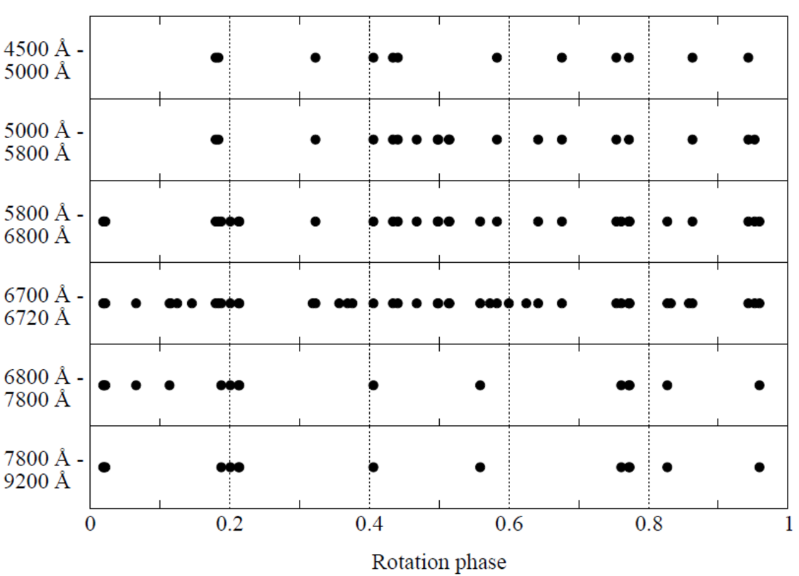
Figure 1: Phase coverage of the data used for Doppler imaging. The different panels show the phase coverage of the several wavelength regions, which changes due to the combination of spectra from various spectrographs and settings (see text).

The relatively large rotational period error, estimated by Maitzen et al., (1980) from the visual examination of light curves, suggests significant uncertainties in the phase calculation for our spectroscopic data, making it problematic to relate DI maps to the magnetic and photometric variations. However, Elkin et al., (2008) shows that the phasing of the new and old magnetic field measurements agrees to within 0.05 of the rotational period. This implies a period error of $\approx 6\times 10^{-5}$, which is small enough to be negligible for our analysis and interpretation of the mapping results. Our own estimates of the period accuracy led to a similar value of $\approx 4\times 10^{-5}$.

The resolution of the spectra ranges from $48\,000$ to $115\,000$, as shown in Table 1. For UVES spectra the resolution varies from $95\,000$ for the blue to $115\,000$ for the red arms, when using the narrowest slit width available. Depending on the setting, which is different for all the UVES runs, gaps in the spectral coverage occur at different wavelengths. by combining all available observations the resulting phase coverage has a maximum phase gap of $\Delta\phi=0.2$, which is visualized in Fig. 1.

Basic data reduction was performed with pipelines of the corresponding instruments^,. For the Mt Stromlo and FEROS data, the reduction was done with the Image Reduction and Analysis Facility (IRAF, Tody, (1986)) and standard recipes.

Additional Strömgren and Johnson photometry was used and is summarized in Table  3.

3 Basic methods

Over the course of this work two different model atmosphere codes were used iteratively. As a starting point, ATLAS9 model atmospheres (Kurucz, 1992, 1993)were computed because the use of opacity tables allows for very fast calculations. An initial abundance analysis was performed based on equivalent widths and individual line profile fitting in the case of blended lines. For further analysis LLmodels model atmospheres (Shulyak et al., 2004) were considered a more appropriate choice for a star with a rather complex abundance pattern such as for HD 3980. The LLmodels code was used to construct a final model atmosphere with the individual abundances presented in Fig. 2. If elements were found to be inhomogeneously distributed across the stellar surface, average homogeneous abundance values were implemented in the model atmosphere calculations.

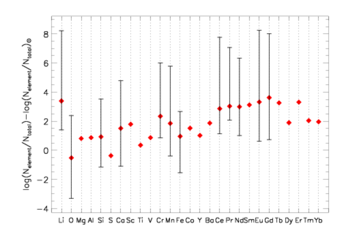
Figure 2: Elemental abundances of HD 3980 relative to the Sun. Vertical bars are attached to mapped elements and correspond to maximum and minimum surface abundances as shown in abundance maps (see Sect. 4 for more details, Figs. 4, 5, and 6). Reference solar abundances are from Asplund et al., (2005).

To calculate synthetic spectra the Synth3 code described by Kochukhov, (2007) was used. The list of atomic lines used in our study was taken from the VALD data base (Piskunov et al., 1995; Kupka et al., 1999). Further information on the final linelist used for reconstructing abundance maps is given in the Table 2.

Table 2: Table of elements and spectral lines from VALD used for mapping HD 3980.

Species	$\lambda$, Å	$\log(gf)$	$E_{\rm low}$, eV	Blended with
Mn ii	4737.9440	-2.940	6.128
Mn ii	4738.2900	-1.876	5.380
Ce ii	5518.3580	-2.030	0.553
Ce ii	5518.4570	-2.000	1.482
Ce ii	5518.4890	-0.670	1.155
Ce ii	5518.6030	-2.430	1.079
La ii	5880.6330	-1.830	0.235	Cr
Gd ii	5855.2150	-1.020	1.598
Gd ii	6004.5590	-0.780	1.659
Fe i	6065.4820	-1.530	2.608
Fe i	6230.7230	-1.281	2.559	Ce
Cr ii	6176.9810	-2.887	4.750
Cr ii	6177.2060	-3.093	6.686
Cr ii	6379.7920	-3.767	4.497	Fe, Gd
Cr ii	6226.6380	-3.035	4.756	Ce
Eu ii	6437.6400	-0.320	1.320
Ca i	6439.0750	0.390	2.526
Li i	6707.7561	-0.440	0.000	Ce, Pr, Sm
Li i	6707.7682	-0.239	0.000
Li i	6707.9066	-0.965	0.000
Li i	6707.9080	-1.194	0.000
Li i	6707.9187	-0.745	0.000
Li i	6707.9200	-0.965	0.000
Nd iii	6145.0677	-1.330	0.296	Si, Ca
O i	7771.9413	0.369	9.146	Cr
O i	7774.1607	0.223	9.146	Nd, Gd
O i	7775.3904	0.001	9.146
Pr iii	7781.9830	-1.210	0.000	Fe, Gd
Si i	7932.3480	-0.468	5.964
Si i	7944.0010	-0.293	5.984	Cr

The observed line profiles were inverted with the INVERS12 code (Kochukhov et al., 2004). The code uses a regularized minimization algorithm and can treat many individual lines and their blends simultaneously. A detailed description of the software and some practical applications are given by, e.g., Piskunov & Rice, (1993),Lüftinger et al., (2010), and Kochukhov et al., (2004).

4 Results

4.1 Fundamental parameters

The TempLogG^TNG program (Kaiser, 2006) was used to derive fundamental parameters from photometric calibrations (Moon & Dworetsky, 1985). The available Johnson $V$ and Strömgrem photometry yields $T_{\rm eff}=8340$ K and $\log g=4.3$, but without any error estimation.

This initial estimation was followed by an attempt to determine $T_{\rm eff}$ and $\log g$ by fitting the H$\alpha$ line with a synthetic line profile, which was, unfortunately, not successful owing to large differences between the H$\alpha$ line profiles of the various spectra. No trend that correlates those changes to the rotational period was found. It is possible that these variations are caused by the reduction pipelines, the continuum fitting procedure, or the curvature of the echelle spectra.

As reported in Obbrugger et al., (2008), the temperature was previously estimated to be $8500$ K. This value was based on equivalent width measurements of several Fe i and Fe ii lines, which also yielded $\log g=4.0$. Previous publications give several rather similar values for the temperature, e.g., $8000\pm 250$ K (Drake et al., 2004), $8270\pm 200$ K (Kochukhov & Bagnulo, 2006), or $8240\pm 300$ K (Hubrig et al., 2007). The $\log g$ values published so far are $4.04\pm 0.05$ from Drake et al., (2004), $4.05\pm 0.09$ in Hubrig et al., (2007), and $4.0\pm 0.2$ by Elkin et al., (2008). Consequently, $T_{\rm eff}=8300\pm 250$ K and $\log g=4.0\pm 0.2$ were adopted for the Doppler mapping procedure in this work.

The absolute magnitude of the star was calculated using the new reduction of Hipparcos data. Stellar luminosity and radius were computed with the bolometric correction from Landstreet et al., (2007).

The value of the projected rotational velocity $\upsilon\sin i$ was determined by comparing of the synthetic spectra with observations of magnetically insensitive iron lines. This method led to a $\upsilon\sin i$$=22.5\pm 2$ km/s. Combination of the measured $\upsilon\sin i$, period, and radius results in an inclination angle of $i<44$ degrees.

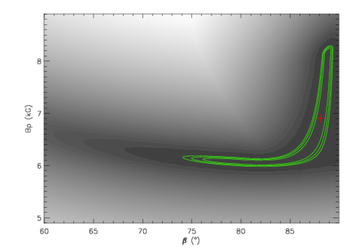
Figure 3: Chi-square surface as a function of dipolar strength ($B_{\rm p}$) and magnetic obliquity ($\beta$). The cross marks the best-fit solution, while the contours correspond to the $1$, $2$, $3$ sigma limits. The uncertainty of the inclination angle is taken into account implicitly. For each $B_{\rm p}$-$\beta$ pair the lowest chi-square was recorded, varying inclination within its $\pm 1$ sigma range in ${\rm sin}\leavevmode\nobreak\ i$.

Magnetic field measurements for this star have been reported by Maitzen et al., (1980), Hubrig et al., (2006) and Elkin et al., (2008). Since only measurements of the longitudinal magnetic field $\langle B_{\rm l}\rangle$ are presently available, the magnetic field geometry is assumed to be a centered dipole (which is usually a good approximation in the case of magnetic A stars). Using a relation between the maximum and minimum of the longitudinal magnetic field and inclination angle $i$ (see Preston, 1967), an angle $\beta=88^{\circ}$ was therefore found between the line-of-sight and the rotation axis of the star. From the fit to the measurements of the mean longitudinal field Elkin et al., (2008) obtained an amplitude of $1904$ G. The positive magnetic pole is located near the zero rotational phase (light minimum).

Because of the relatively small error in the period estimated by Elkin et al., (2008), we do not expect large changes in the position of the magnetic extrema. This conclusion also follows from Fig. 2 of Elkin et al., (2008), which illustrates a good match between the two magnetic measurements from different epochs (1980 and 2006) folded with the same period. Last but not least, the most recent magnetic measurements cited in Elkin et al., (2008) and our spectroscopic measurements overlap in time, thus justifying the use of the ephemeris from Maitzen et al., (1980). Finally, using the relation from Preston, (1967), which combines the amplitude of the longitudinal magnetic field variation, inclination angle, magnetic angles, and limb-darkening coefficient (assuming $u=0.5$), we obtain the polar strength of the dipolar field $B_{\rm p}\approx 7$ kG. Taking the uncertainty of the inclination angle into account, the 1 sigma confidence ranges of these parameters are $B_{\rm p}=6.01-8.25$ kG and $\beta=76^{\circ}-89^{\circ}$. Figure 3 illustrates the analysis of the $B_{\rm z}$ measurements for HD 3980, showing the chi-square surface as a function of dipolar strength ($B_{\rm p}$) and magnetic obliquity ($\beta$).

Table 3: Fundamental and atmospheric parameters of HD 3980 used for Doppler imaging.

Parameter	Value	Reference
$H_{\beta}$	2.870	(1)
$b-y$	$0.070\pm 0.007$	(1)
$m1$	$0.296\pm 0.007$	(1)
$c1$	$0.748\pm 0.022$	(1)
$V$	$5.71\pm 0.005$	(1)
$\pi$, mas	$14.91\pm 0.35$	(2)
$d$, pc	$67.07\pm 1.57$	(2)
$BC$, mag	$0.6\pm 0.07$	(3)
$M_{\rm bol}$, mag	$1.64\pm 0.079$
$\log(L/L_{\odot})$	$1.24\pm 0.04$
$R/R_{\odot}$	$2.04\pm 0.26$
$\upsilon\sin i$, km/s	$22.5\pm 5$
$i$, ∘	60 (14-90)
$\beta$, deg	88.1 (76-89)
$B_{\rm p}$, kG	6.9 (6.0-8.3)
$T_{\rm eff}$, K	$8300\pm 250$
$\log g$, cgs	$4.0\pm 0.2$
Photometric measurements were taken from 1:
Hauck & Mermilliod, (1998), 2: van Leeuwen, (2007),
3: Landstreet et al., (2007).

All photometric measurements and resulting fundamental parameters of HD 3980 are summarized in Table 3.

4.2 Surface abundance distributions

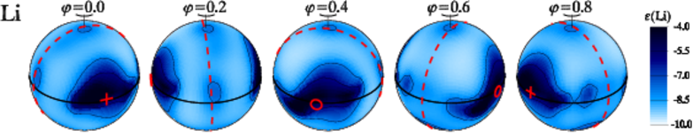
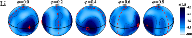
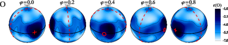
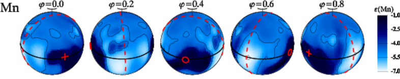
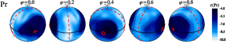
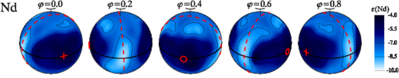
Figure 4: Abundance distributions of Li, O, Mn, Pr, and Nd at the surface of HD 3980 obtained from the lines listed in Table 2. The star is shown at five rotational phases. Darker areas correspond to the higher elemental abundances, the corresponding scale is given to the right of each panel and contours with equal abundances are plotted with steps of $1$ dex. The circle and the cross indicate the position of the negative and the positive magnetic poles, respectively. This figure represents elements of Group 1 with enhanced spots centered on the magnetic poles. Two Li maps correspond (from top to bottom) to the cases of simultaneous mapping of Li i and Pr iii blend at $6707$ Å, and additional implementation of Pr iii $7781.983$ Å line (see text). Abundances are given in $\log(N_{\rm el}/N_{\rm total})$.

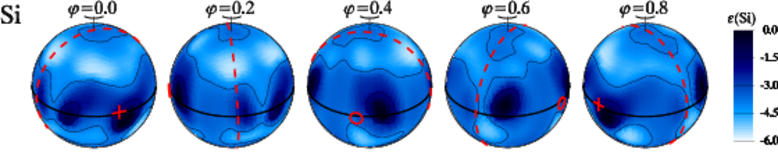
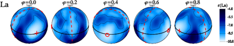
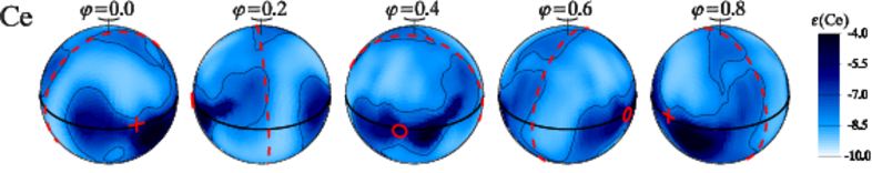
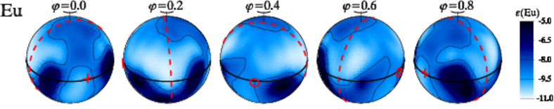
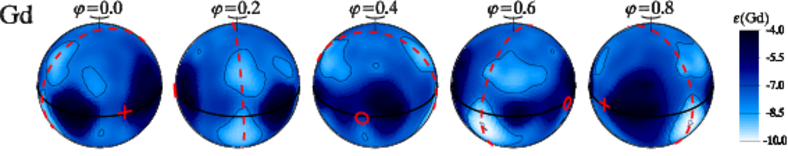
Figure 5: Same as on Fig. 4, but for Si, La, Ce, Eu, and Gd. This figure represents elements of Group 2 with spots of higher abundance between the magnetic poles and the magnetic equator.

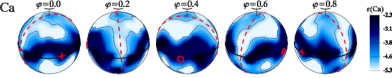
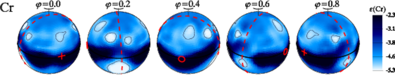
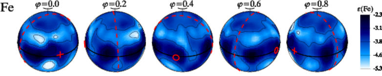
Figure 6: Same as on Fig. 4, but for Ca, Cr, and Fe. This figure represents elements of Group 3 with overabundances in the area of the magnetic poles along the rotational equator.

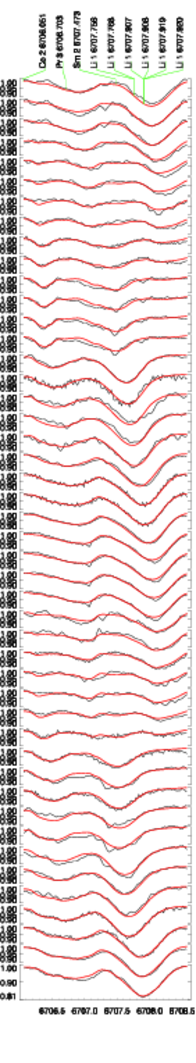
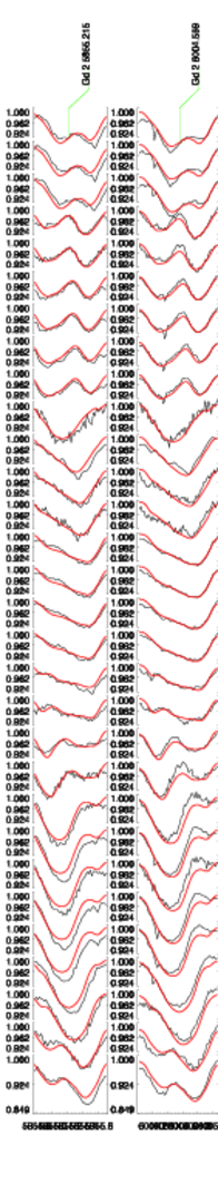
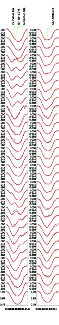
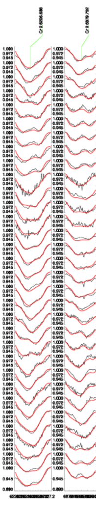
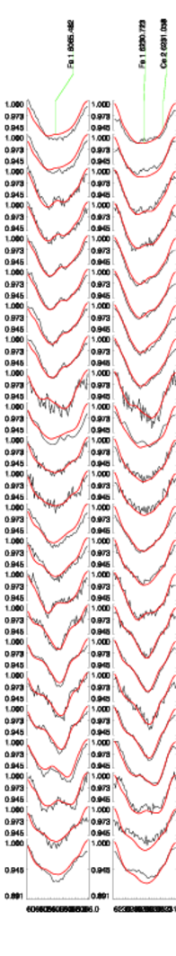
Figure 7: Examples of observed and predicted phase-dependent profiles of selected elements computed from the respective abundance maps shown in Figs. 4, 5, and 6.

In the following we give a short overview of the results for each individual element that has been mapped. Abundance maps are combined in three groups according to the distribution pattern and its link to the assumed magnetic field geometry. These maps are presented in Figs. 4, 5, and 6 (see Sect. 5). Examples of the theoretical fits to phase-resolved profiles of some selected lines are presented in Fig. 7 for illustration. When comparing the magnitude of over- or underabundance of some elements we assume reference solar abundances from Asplund et al., (2005). In all other cases (if not explicitly stated), when referring to the abundances of particular surface region, enhancements or depletion is discussed relative to the mean surface abundance.

Lithium

This map has the highest phase coverage ever used for Doppler imaging of an A-type star. Forty-six phases were available to reconstruct the abundance variations of Li (see Fig. 1). Pr iii at $6706.703$ Å was varied simultaneously, because the overlap in wavelength occurred when Li and Pr spots were visible near the stellar limb. The enhancements of Li at the magnetic poles have an overabundance of $\approx 5$ dex compared to the Sun. The solar abundance of Li is $\approx 2$ dex lower than the initial cosmic abundance, (Baumann et al., 2010).

An additional parallel implementation of Pr iii at $7781.983$ Å leads to a more extended concentric Li spot around the magnetic poles with the same overabundance of $\approx 5$ dex (see Fig. 4, second plot from top). The enhancement at the negative pole was slightly shifted towards a higher longitude, but resulting in slightly worse fit to the Pr iii line at $6706.703$ Å. This could be due to influences of the Sm ii line at $6707.473$ Å or Ce ii $6706.051$ Å and $6708.099$ Å lines that were only accounted for as having a constant abundance over the whole stellar surface (see, e.g., Drake et al., 2005).

Oxygen

The surface abundance pattern of oxygen was reconstructed using the triplet at $7770$ Å. The line profile variations are very pronounced and reproduced well in the area of these three O lines. Blends of Nd and Gd were included with constant abundance contribution. Like Li, O is concentrated in two spots at the magnetic poles, whereas the enhancement at the negative pole is also shifted towards a higher longitude. Around the magnetic field equator oxygen appears rather depleted. Oxygen abundance maps have so far been reported for the hotter Ap star $\epsilon$ UMa (Rice et al. 1997) and for HD 83368 (HR 3831), with a comparable temperature to HD 3980 (Kochukhov et al., 2004). It is interesting to note that the distribution of oxygen abundance in HD 3980 is completely different from what is observed in the two other stars, where oxygen is strongly concentrated in the region of the magnetic equator.

Silicon

In order to derive the abundance pattern of Si, two Si ii lines at $7932.348$ Å and $7944.001$ Å were combined, where the weak Cr ii $7944.527$ Å blend was implemented by assuming a constant abundance over the rotation period. Our results indicate that there are several spots of overabundance around the rotational equator in the area between the magnetic poles and the magnetic equator.

Calcium

The Ca surface distribution was obtained by combining the unblended Ca i line at $6439.075$ Å with the Nd iii, Ca ii, and Si i blend at $6145$ Å. Since all elements contribute strongly to the blend, their distribution was determined simultaneously in this calculation. The resulting surface image of Ca shows an overabundance in the region of the rotational equator and in the area of the magnetic poles of more than $2$ dex compared to the Sun and displays approximately solar abundance around the magnetic equator.

Chromium

Chromium shows a very distinct structure of an overabundance around the rotational equator broken by an underabundance around the magnetic equator. To minimize the effects of possible vertical abundance stratification (frequently found in roAp stars, Shulyak et al., (2009)), two lines of the same ion with the similar excitation energy were used (Cr ii $6226.638$ Å and Cr ii $6379.792$ Å).

Manganese

Two lines of Mn ii at $4737.944$ Å and $4738.290$ Å were used. Due to the spectral coverage in this region, only 12 phases are available, but the phases are evenly spaced over the rotational cycle. The surface distribution of manganese is characterized by two patches of enhanced abundance around the magnetic poles and depletion at the intersections of the magnetic and rotational equators.

Iron

Two Fe i lines at $6065.482$ Å and $6230.723$ Å have very similar excitation energy and are practically unblended. The Ce ii line at $6231.058$ Å was taken into account by assuming a constant abundance. Iron is distributed in high-contrast spots of overabundance around the rotational equator, and seems to accumulate at the magnetic poles rather than at the magnetic equator.

Lanthanum

The most remarkable features of the surface distribution of La are the depletion regions around the magnetic poles. The regions with higher abundance are located in the area between the magnetic poles and the magnetic equator, and slightly shifted towards the southern hemisphere.

Cerium

The map resulting from the inversion of the Ce i lines at $5518$ Å shows enhanced abundances in the region between the magnetic poles and the magnetic equator. The area around the magnetic equator itself is depleted.

Praseodymium

The result of the inversion of Pr iii $7781.983$ Å shows that two spots are observed around the magnetic poles with an abundance increase of more than $5$ dex compared to the solar value. Also the area of lowest abundance around the magnetic equator is more than $1$ dex higher than for the Sun.

We found that the combination of the Li line at $6708$ Å with the Pr iii $7781.983$ Å line results in a very similar distribution that shows two patches in the area of the magnetic poles, but their centers are shifted by $+20^{\circ}$ in longitude. The spot size, as well as the abundance value, agree, which is also valid for the depletion surrounding the magnetic equator. As mentioned before, the praseodymium line contributing to the Li-Pr blend at $6708$ Å is rather weak. We therefore kept only the map resulting from the Pr iii $7781.983$ Å line.

Neodymium

Neodymium was – similar to Ca – derived from the combination of the Ca ii, Si i, and Nd iii blend at $6145$ Å and Ca i line at $6439.075$ Å; however, the contribution of Ca ii and Si i appeared to be weak. The map shows a depletion surrounding the magnetic equator. Similar to Pr, two concentric areas of higher abundance are centered on the magnetic poles.

Europium

Just like Ce, the enhanced regions of Eu are situated between the magnetic equator and the magnetic poles. The two main spots are shifted towards higher longitudes relative to the magnetic poles.

Gadolinium

Gadolinium shows enhanced spots in the area of the rotational equator. Around the magnetic equator, several spots of lower abundance are visible. The enhanced areas are located between the magnetic poles and the magnetic equator. This surface abundance distribution was derived by combining the two Gd ii lines at $5855.215$ Å and $6004.559$ Å.

5 Discussion

5.1 Magnetic spectrum synthesis and abundance maps

In the present Doppler imaging analysis we used a nonmagnetic spectrum synthesis for computating the line profiles of respective elements. However, with a polar magnetic field strength of up to $7$ kG and magnetic angle $\beta=88^{\circ}$, the mean surface magnetic field modulus ranges from $4.5$ kG to $5.4$ kG during the rotation period. Such a magnetic field is strong enough to influence the line profiles , so that its possible impact on the abundance maps has to be discussed.

It is known that the formation of the Li i $6707.473$ Å line is subject to the Paschen-Back effect (see Kochukhov, 2008a ; Stift et al., 2008), which becomes noticeable around $3$ kG. However, we did not account for this in the present study because a) modeling the Paschen-Back effect is a non-trivial task that requires special software and complex techniques; b) the true geometry of the global magnetic field of HD 3980 is not known, i.e. its deviation from the simple dipole would introduce additional uncertainties in the line profile fitting with magnetic spectrum synthesis, and c) the star’s rather high $\upsilon\sin i$$=22.5$ km/s smears out the line profile shape considerably.

To estimate the impact of neglecting the magnetic field in spectrum synthesis on the derived abundances, especially of strongly overabundant elements, we used the Synth3 and Synthmag codes (Kochukhov, 2007) to calculate two sets of synthetic spectra for the lines of Fe, Cr, Eu, and Gd which are most sensitive to the magnetic field i) without magnetic field, and ii) considering a magnetic field modulus of $5$ kG. For both cases synthetic profiles were fit to observed lines in a rotation phase close to maximum abundance. We found that including the Zeeman splitting in the presence of a magnetic field leads to an abundance decrease of $0.10-0.15$ dex for Fe and Cr. For the Eu line, in addition to the Zeeman splitting, isotopic splitting and hyperfine structure were also taken into account in magnetic spectrum synthesis. A terrestrial Eu isotopic composition was adopted. Due to this complex pattern of the Eu II $\lambda$ $6437$ line used for mapping, the abundance decreased by $0.65$ dex compared to the simplified, nonmagnetic case. The highest abundance difference was derived for Gd. A large Landé factor and a complex Zeeman pattern meant its abundance in the magnetic case had to be decreased by $1.1$ dex to fit observations. Except for Eu and Gd, the upper abundance limits of the maps computed with INVERS12 are not very affected by neglecting the magnetic field. Lower abundance limits are not influenced as much for any of the lines used for mapping.

Finally, it is important to understand that more accurate work could be done by applying a magnetic Doppler imaging when both distributions of the magnetic field and abundances are mapped simultaneously. This, of course, will become possible once additional polarimetric observations are available.

5.2 Surface patterns and assumed magnetic field geometry

As noted in Sect. 4, the single-wave variations in the longitudinal magnetic field of HD 3980 can correspond to the magnetic dipole with the obliquity angle $\beta=88^{\circ}$. The true magnetic field configuration can, of course, be more complex. But since no phase-resolved observations of additional magnetic parameters (e.g. field modulus $|\mathrm{\mathbf{B}}|$) are available, it is currently impossible to determine the magnetic field topology precisely. Nevertheless, assuming that the magnetic field is dominated by a dipolar-like configuration (which is commonly found in other A-type magnetic stars), we can look for a link between the global magnetic field geometry and elemental abundance distributions.

The elements displayed in Fig. 4 show more or less circular regions of higher abundance around the magnetic poles (Group 1). Especially around the negative magnetic pole, a shift in the enhanced spot towards higher longitudes is visible. Besides Pr and Nd, lighter elements such as Li, O, and Mn – an iron peak element – are also distributed in the same way. The other apparent feature of this group is lower abundance around the magnetic equator.

The next set of elements (Group 2), which are displayed in Fig. 5 shows high abundance regions placed mainly between the magnetic poles and magnetic equator. Lanthanum even avoids the magnetic poles and shows a concentric region of underabundance around them (in contrast to, e.g., O or Pr). The region surrounding the magnetic equator, on the other hand, is dominated by La-depleted areas.

The final Group 3, displayed in Fig. 6, is not as clearly defined, so it cannot be assigned to any of the other groups. Ca, Cr, and Fe are overabundant along the rotational equator and the area of the magnetic poles, but not in circular spots as in the case of, e.g., Li or Nd. The region of the magnetic equator is depleted for all those elements.

Such a distinct separation of the mapped elements into the three groups described above can only be explained once the interplay between rotation, diffusion, and magnetic field is correctly modeled in recent and/or future diffusion models.

5.3 Comparison with diffusion models

Assuming that the magnetic field geometry is a centered dipole, simple structures like rings or caps are expected, according to Michaud et al., (1981). Caps around the magnetic poles are found for Li, O, Mn, Pr, and Nd with depletion around the magnetic equators. The other 8 investigated elements have a more complicated structure. None of the analyzed elements show enhancements around the magnetic equator. But, e.g., Si should be overabundant in areas of close to horizontal magnetic field lines, as stated by Alecian & Vauclair, (1981), Michaud et al., (1981), or Vauclair et al., (1979). The enhanced spots of Si are situated between the magnetic equator and the magnetic poles. This might suggest that the diffusion process is still going on.

To explain surface abundance patterns of Ap stars, a further development of the diffusion theory was proposed by Babel, (1992, 1993, 1995). It is claimed that additional modifications of the outer boundary condition by a small and inhomogeneous mass outflow could considerably modify the surface abundance structure. Ambipolar diffusion of hydrogen in magnetized plasma can also affect surface abundance patterns compared to the predictions of the initial parameter-free diffusion theory where no mass loss or ambipolar diffusion were considered. In particular, for stars with a $T_{\rm eff}$ of more than $10\,000$ K, a mass loss due to radiative pressure is predicted for selected metals (Babel, 1995). Such weak metal winds could produce surface inhomogeneities with varying contrast between the elements. Unfortunately, only a few of the elements investigated in this work were the subject of diffusion calculations, which are so far applicable to a limited range of $T_{\rm eff}$ and $\log g$ values.

The Group 2 of elements (e.g. Fig. 5) especially shows asymmetric distributions and variations of the abundance pattern from one element to the other. So far those cannot be explained by the simplified diffusion models. As stated by Kochukhov et al., (2004), a more complex interaction of rotation, magnetic field, and mass loss might be the solution for that.

Reconstruction of the true magnetic geometry of HD 3980 by means of magnetic Doppler imaging (against a simplified pure dipolar geometry assumed in this work) is the next necessary step. Such an analysis will certainly provide us with deeper insight into the connection between location of the magnetic poles, their strengths, and distributions of chemical elements.

6 Conclusions

The spectrum analysis of HD 3980 was carried out in order to determine atmospheric parameters for Doppler imaging. By assuming a centered dipolar magnetic field, the inclination of rotational axis to the magnetic field axis was determined to be close to $88^{\circ}$. Longitudinal magnetic field variation implies a dipolar field with a polar strength of $B_{\rm p}\approx 7$ kG.

Horizontal inhomogeneities were detected and investigated using the Doppler imaging code INVERS12. However, this was done without direct incorporation of the magnetic field into the spectrum synthesis calculation. The resulting maps were summarized in three groups corresponding to the association of the surface patterns and their relation to the magnetic field.

Lithium, O, Mn, Pd and Nd are mainly concentrated in the area of the magnetic poles and depleted in the regions around the magnetic equator. The high abundance spots of Si, La, Ce, Eu, and Gd are located between the magnetic poles and the magnetic equator. Except for La, which is clearly depleted in the area of the magnetic poles, no obvious other correlation with the magnetic field has been found for these elements. Ca, Cr, and Fe show enhancements at the magnetic poles, but also along the rotational equator. The intersection between the magnetic and the rotational equator constitutes an exception, especially for Ca and Cr, which are depleted in that region.

No obvious correlation between theoretical predictions of diffusion in CP stars and the abundance patterns could be found. This is likely attributed to a lack of up-to-date theoretical models. For elements like O or Ca, belts of enhanced abundance around the magnetic equator are predicted, but not present in all CP stars. Unlike some CP stars, including HD 3980 analyzed in this paper, O is concentrated around the magnetic poles.

Finally, to complete the investigation of the abundance structures in the atmospheric layers of the HD 3980, further investigations will be pointed toward the accurate reconstruction of the surface magnetic field configuration and expected vertical abundance gradients will be investigated and modeled.