Probing two approaches to Unified Dark Dynamics

Abstract

Dark matter and dark energy are essential in the description of the late Universe, since at least the epoch of equality. On the other hand, the inflation is also necessary and demands a ”dark” component, usually associated to a scalar field that dominated the dynamics and kinematics in the very early Universe. Yet, these three dark components of standard model of cosmology are independent from each other, although there are alternative models that pursue to achieve a triple unification, or at least a double. In the present work we present an update of two models that we have considered in recent years. The first is the dark fluid model in which dark matter and dark energy are the same thing, achieving a double unification with specific properties that exactly emulate the standard model of cosmology, given the dark degeneracy that exists in the $\Lambda$CDM model. The second model is given by a single $F(X)$ scalar field Lagrangian, with which one is able to model the whole cosmological dynamics, from inflation to today, representing a triple unification model. We highlight the main properties of these models, as well as we test them against known cosmological probes.

1 Introduction

The standard model of cosmology is based on the existence of dark matter and dark energy, apart from the particle content of standard model of particle physics, see ref. Cervantes-Cota and Smoot (2011) for a short review. These dark components have been dominating the dynamics and kinematics since at least the equality epoch, when non-relativistic matter dominated over the relativistic components, and they are essential to understand the evolution of both the background and the perturbed cosmos. However, we have not yet a definitive knowledge of their origin nor strong clues on what relationship the dark components could have among each other. It is suspected that they might share a common origin since the amount of dark matter and dark energy is of the same order of magnitude today ($\Omega_{m}\approx\frac{1}{3}\Omega_{de}$), a fact known as coincidence problem Chimento et al. (2003).

On the other hand, the standard model of cosmology includes an inflationary dynamics at very early times that is important mainly to solve the old long-standing puzzles (the horizon and flatness problems and a causal origin of perturbation seeds). This accelerated dynamics implies the existence of another ”dark” (not yet seen) component that is thought to be due to some scalar field dynamics. The scalar field is then presumed, in (pre-) re-heating, to be converted into bosons and fermions that made the Universe material.

Given the above facts, one identifies three dark (unknown) components of the Universe: dark matter, dark energy, and the inflationary energy. Do they have a common origin? or least a couple of them? These are questions that have had many answers, as many as a plethora of models in the literature of unified dark components, see for instance Copeland et al. (2006); Bertacca et al. (2010). The task is not simple since we are treating here with very different energy scales. By comparing for instance the energy scale of inflation and that of dark energy, that in the limiting case if inflation would have happened at the Planck scale, $\rho_{\rm inflation}\sim 10^{122}\rho_{de}$; the most standard energy scale of inflation ($\rho_{\rm inflation}\sim(10^{15}{\rm GeV})^{4}$) subtracts only 16 orders magnitude to that difference. On the other hand, if reheating took place at the end of inflation, the oscillating scalar field behaves as a dust gas ($p=0$) Turner (1983). The key issue to identify it with dark matter is that the reheating process must reduce the field density enough to make it subdominant during the radiation epoch, but not completely, for it to account for the right proportion today ($\Omega_{dm}\sim 0.2-0.3$), something that proved to be nontrivial to achieve in standard reheating schemes Kofman et al. (1997); Liddle and Urena-Lopez (2006).

The above facts indicate some of the difficulties to perform a unification of the different dark components of the Universe. In pursuing it, we would like to stress the following simple properties of these components that have led us to propose two different models of unification. Let us start mentioning that from the dynamical point of view one needs a dark matter fluid with negligible pressure ($p\ll\rho$, and in fact in the standard model $p=0$). As a second property, one requires to have the right proportion of dark matter to baryons, $\frac{\Omega_{dm}}{\Omega_{b}}\approx 5$ Hinshaw et al. (2012). A third property is that the kinematics of dark matter is such that yields potential wells, from astrophysical to cosmological scales. This in turn implies that the effective speed of sound of dark matter is $c_{s}\ll c$, and in fact in the standard model $c_{s}=0$. About dark energy we want to remark also three properties: First, it has a particular energy scale, $\rho_{de}$, that dominates the background dynamics over all other components since a recent redshift $z\approx 0.5$ Busca et al. (2012). Second, it has a pressure proportional to its density $p=-\rho_{de}$, and third, it does not seem to cluster in sub-horizon scales. Finally, the inflation dynamics demands a series of tests to be accomplished, such as to yield a minimum of e-folds of expansion, a correct amplitude of density fluctuations, and an almost Harrison-Zel’dovich spectrum ($n_{S}\approx 0.96$); other tests as evading excess of non-Gaussianities and large tensor-to-scalar amplitude of fluctuations are also important, for more details see e.g. ref. Hinshaw et al. (2012).

Based on the above mentioned remarks about the dark components, in the present work we present two different unification approaches that were partially worked out by us in recent years and here we test them further and remark some of their properties. The first model unifies dark matter and dark energy at the most trivial manner, identifying both of them with a single, dark fluid. This is presented in next section, ”The dark fluid”. The second model accomplishes the dynamics of the three dark components with a single scalar field, whose standard quadratic potential is responsible for the inflationary behavior, and later, ”dark matter” domination is achieved through the specific dynamics of scalar field whose non-trivial kinetic term possesses a minimum. Finally, dark energy is realized by adding a proper (but not the standard) cosmological constant to the model. The later model is present in section ”Non-standard scalar field unification”. Last, we present our conclusions at the end of the manuscript.

2 The dark fluid

As we mentioned, the dark components of the Universe are decomposed, within the standard model of cosmology, in dark matter and dark energy. However, this is only a possibility that in fact has support from historical reasons, but there are more ways to understand the dark sector, and specifically, in a unified way. Perhaps the simplest unified description of dark matter and dark energy is given by the so-called dark fluid. It is defined in a first approximation as a barotropic perfect fluid with adiabatic speed of sound equals to zero Aviles and Cervantes-Cota (2011a) (see also Luongo and Quevedo (2011)),

$$c^{2}_{s}=0.$$ (1)

Being the fluid barotropic, this last condition implies that its perturbations do not develop acoustic oscillations, and therefore they grow at all scales by gravitational instabilities, behaving as cold dark matter. Several extensions to this model can be found in the literature, see for example Balbi et al. (2007); Xu et al. (2012); Caplar and Stefancic (2013); Aviles et al. (2012). Without lost of generality we can write the equation of state of the dark fluid as

$$P_{d}(\rho_{d})=w_{d}(\rho_{d})\rho_{d},$$ (2)

where we have factorized the equation of state parameter $w_{d}$, which is a function only of the energy density of the fluid. From $c_{s}^{2}=(\partial P/\partial\rho)_{s}=dP/d\rho$, equations (1) and (2) imply that $w_{d}(\rho)+\rho_{d}dw_{d}(\rho_{d})/d\rho_{d}=0$, and then $w_{d}(\rho_{d})=-C/\rho_{d}$ where $C$ is a constant and the negative sign has been chosen for future convenience. From now on we will denote with a subindex d the variables of this dark fluid. The pressure is then

$$P_{d}=-C.$$ (3)

Thus, although the dark fluid perturbations grow at all scales, it is allowed to have a non-zero pressure. Astrophysical observations constrain this value to be very small, $|P|\ll\rho_{A}$, where $\rho_{A}$ is the energy density of typical astrophysical scales where dark matter has been detected. Usually, it is assumed that dark matter is pressureless, but this is by not means necessary, for instance it could be the case that $|P|\sim\rho_{c0}$, where $\rho_{c0}$ is a typical cosmological energy density scale at present, without getting in contradiction with observations. In fact, this is the entrance that leads us to consider the dark fluid to be dark energy as well as dark matter.

Now, let us consider a homogeneous and isotropic Universe at very large scales whose geometry is described by the Friedmann-Robertson-Walker metric, and that is filled with standard model particles ($b$, $\gamma$, …) and with the above-defined dark fluid. The evolution equations of such a Universe are

$$H^{2}=\frac{8\pi G}{3}(\rho_{d}+\rho_{b}+\rho_{\gamma}),$$ (4)

$$\rho_{b}^{\prime}+3H\rho_{b}=0,$$ (5)

$$\rho_{\gamma}^{\prime}+4H\rho_{\gamma}=0,$$ (6)

and

$$\rho_{d}^{\prime}+3H(1+w_{d})\rho_{d}=0,$$ (7)

where prime means derivative with respect to cosmic time and $H\equiv a^{\prime}/a$ is the Hubble factor. Equations (5) and (6) give $\rho_{b}=\rho_{b0}a^{-3}$ and $\rho_{\gamma}=\rho_{\gamma 0}a^{-4}$, where a subindex $0$ stands for quantities evaluated at present time, and we have normalized the scale factor to be equal to one today, $a_{0}=1$. Integration of equation (7) gives

$$\rho_{d}=\frac{\rho_{d0}}{1+\mathcal{K}}\left(1+\frac{\mathcal{K}}{a^{3}}\right),$$ (8)

where we have defined the constant $\mathcal{K}=(\rho_{d0}-C)/C$. This expression is exactly what one expects for a unified fluid: it contains a constant piece that behaves as dark energy and a second term that decays with the third power of the scale factor, just as a dark matter component does.

Now, the equation of state parameter of the dark fluid becomes

$$w_{d}=-\frac{1}{1+\mathcal{K}a^{-3}}.$$ (9)

and its pressure, expressed in terms of the constant $\mathcal{K}$ instead of $C$, is

$$P_{d}=-\frac{\rho_{d0}}{1+\mathcal{K}}.$$ (10)

In order to ensure the positivity of the energy density at all times, the constant $\mathcal{K}$ must be a positive number. This implies that the pressure is negative, a quality that allows the dark fluid to accelerate the Universe, and as we have outlined above it could take values of the order of the critical density $(\sim 3H_{0}^{2}/8\pi G)$ without affecting the behavior of the dark fluid as dark matter in astrophysical scenarios.

In the $\Lambda$CDM model the equation of state parameter of the total dark sector, $w_{T}$, defined by

$$w_{T}\equiv\frac{\sum_{a}w_{a}\rho_{a}}{\sum_{a}\rho_{a}},$$ (11)

where the subindex $a$ runs over dark matter (DM) and cosmological constant ($\Lambda$), is given by

$$w_{T}=-\frac{1}{1+\frac{\Omega_{DM}}{\Omega_{\Lambda}}a^{-3}}.$$ (12)

(Note that in our convention $\Omega_{i}$ refers to the $i$-component abundance evaluated at present time.) Comparing these results to equations (4), (8), and (9) we note that under the identifications

$$\mathcal{K}=\frac{\Omega_{DM}}{\Omega_{\Lambda}},$$ (13)

and

$$\Omega_{d}=\Omega_{DM}+\Omega_{\Lambda},$$ (14)

the resulting cosmological background evolution in both models is exactly the same. What we have shown is that the dark fluid model is indistinguishable from the $\Lambda$CDM model at the background level. In the next subsection we shall show that these ideas can be extended for a complete cosmological description.

This property has been called dark degeneracy by Martin Kunz in Kunz (2009). In fact, it is more general than for the single fluid case worked here: any collection of fluids whose total equation of state parameter is equal to equation (12) and that do not interact with baryons and photons will behave exactly as the composed dark matter-cosmological constant fluid, leading to a degeneracy with the $\Lambda$CDM model.

2.1 Cosmological perturbations

Now, let us consider cosmological perturbation theory in the conformal Newtonian gauge, the metric is given by (for details and notation see Aviles and Cervantes-Cota (2011a); Ma and Bertschinger (1995))

$$ds^{2}=a^{2}(\tau)\big{[}-(1+2\Psi)d\tau^{2}+(1-2\Phi)\delta_{ij}dx^{i}dx^{j}\,\big{]},$$ (15)

where $\tau$ is the conformal time related to the cosmic time by $dt=ad\tau$. The hydrodynamical equations in Fourier space for the dark fluid, obtained from $\nabla_{\mu}T^{\mu\nu}=0$, are given by

$$\dot{\delta}_{d} = -(1+w_{d})(\theta_{d}-3\dot{\Phi})+3\mathcal{H}w_{d}\delta_{d}-3\mathcal{H}\frac{\delta P_{d}}{\delta\rho_{d}}\delta_{d},$$ (16)

$$\dot{\theta}_{d} = -\mathcal{H}\theta_{d}+k^{2}\Psi+\frac{\delta P_{d}/\delta\rho_{d}}{1+w_{d}}k^{2}\delta_{d}-k^{2}\sigma_{d},$$ (17)

where $\delta$ is the density contrast, $\theta$ the divergence of the peculiar velocity, and $\sigma$ the scalar anisotropic stress. For baryons after recombination, when the coupling to photons can be safety neglected, the hydrodynamical equations are

$$\dot{\delta}_{b} = -\theta_{b}+3\dot{\Phi},$$ (18)

$$\dot{\theta}_{b} = -\mathcal{H}\theta_{b}+k^{2}\Psi.$$ (19)

The fluid equations are supplemented with the Einstein’s equations

$$k^{2}\Phi=-4\pi Ga^{2}\sum_{i}\rho_{i}\Delta_{i},$$ (20)

and

$$k^{2}(\Phi-\Psi)=12\pi Ga^{2}\sum_{i}(\rho_{i}+P_{i})\sigma_{i}$$ (21)

where the sum runs over all fluid contributions and

$$\Delta_{i}=\delta_{i}+3\mathcal{H}(1+w_{i})\frac{\theta_{i}}{k^{2}}$$ (22)

is the rest fluid energy density Bardeen (1980).

To solve these equations, we need to add information about the nature of the dark fluid. The barotropic condition implies that $\delta P=c^{2}_{s}\delta\rho$ and, after equation (1), thus $\delta P_{d}=0$, and because it is a perfect fluid, the anisotropic stress vanishes, $\sigma_{d}=0$. Therefore, in the right-hand side (rhs) of equation (16) the last term vanishes, and in the rhs of equation (17) only the two first terms survive. Moreover, if we solve only for baryons and the dark fluid the two gravitational potentials are equal, $\Psi=\Phi$.

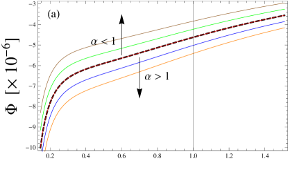
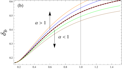
Figure 1: Evolution of perturbation variables for a mode $k=0.05\,\rm{Mpc}^{-1}$. Solid curves are obtained from the dark fluid model for different values of the parameter $\alpha$ in the initial conditions $\delta_{d}(\tau_{i})=\alpha\rho_{\rm{DM}}(\tau_{i})\delta_{\rm{DM}}(\tau_{i})/\rho_{d}(\tau_{i})$. $\alpha$ takes values from 0.8 to 1.2. Dashed curves are for the $\Lambda$CDM model variables. The panels show: (a) Gravitational potential $\Phi$. (b) Baryonic density contrast $\delta_{b}$. (c) Dark fluid (solid lines) and dark matter (dashed line) density contrasts, $\delta_{d}$ and $\delta_{\rm{DM}}$. (d) Dark fluid (solid lines) and dark matter (dashed line) velocities, $\theta_{d}$ and $\theta_{\rm{DM}}$. The solutions for the case $\alpha=1$ are depicted with the thick (red) lines, which for panels (a), (b), and (d) coincide with the dashed lines.

Figure 1 shows the evolution of a mode $k=0.05\,\rm{Mpc}^{-1}$ of the perturbations variables. The dashed lines shows results for the $\Lambda$CDM model, for which we have used the standard dark matter hydrodynamical perturbations equations instead of equations (16) and (17).

In evolving the perturbations for both models, $\Lambda$CDM and dark fluid, we have imposed on the initial conditions the relations $\delta_{d}(\tau_{i})=\alpha\rho_{\rm{DM}}(\tau_{i})\delta_{\rm{DM}}(\tau_{i})/\rho_{d}(\tau_{i})$ for the density contrasts, and $\theta_{d}(\tau_{i})=\alpha\rho_{\rm{DM}}(\tau_{i})\theta_{\rm{DM}}(\tau_{i})/(1+w_{d})\rho_{d}(\tau_{i})$ for the velocities, and we let $\alpha$ to take different values. These initial conditions are given at an initial time well after recombination, so the relation $\delta_{\rm{DM}}\simeq\delta_{b}$ holds and we can neglect the coupling between baryons and photons.

If we take $\alpha=1$ we note the evolution of the baryonic density contrast is undistinguished in both models. Then, although the cosmological observable is the baryonic matter power spectrum which includes a wide range of wavelengths, Figure 1 suggests that indeed the results are the same for both models for any wavelength. In fact this is true and it is shown in Aviles and Cervantes-Cota (2011a). In the cosmological context, imposing these two initial conditions is equivalent to demand that at first order in perturbation theory, the time-time and time-space components of the perturbed energy momentum tensor of the dark fluid and $\Lambda$CDM models are equal at the given initial time $\tau_{i}$. By the fact that we are using General Relativity which is a theory with a well posed Cauchy problem, it is implied that the conditions will be preserved at all times; thus, equations

$$\rho_{d}\delta_{d}=\rho_{\rm{DM}}\delta_{\rm{DM}},$$ (23)

and

$$\rho_{d}(1+w_{d})\theta_{d}=\rho_{\rm{DM}}\theta_{\rm{DM}}.$$ (24)

hold at anytime.

This analysis shows that the degeneracy between the dark fluid and the $\Lambda$CDM model is preserved at the linear cosmological order. To go beyond the linear order, let us make perturbation expansions to the dark fluid and $\Lambda$CDM energy momentum tensors about the (zero order) background cosmological fluids as

$$T_{\mu\nu}=T_{\mu\nu}^{(0)}+T_{\mu\nu}^{(1)}+T_{\mu\nu}^{(2)}+\cdots.$$ (25)

If the total energy momentum tensors of both models are equal $\,\,\big{(}T_{\mu\nu}^{\,d}=T_{\mu\nu}^{\Lambda\rm{CDM}}\big{)}$, clearly each of the terms in the expansion will be equal as well $\big{(}T_{\mu\nu}^{\,d\,(i)}=T_{\mu\nu}^{\Lambda\rm{CDM}\,(i)}\big{)}$. This argument is correct and it is outlined in Kunz (2009) to argue that the degeneracy is preserved at all orders in perturbation theory.

Nonetheless, we want to stress a different approach: We are affected gravitationally by the total energy momentum tensor, but usually when comparing observations to models we expand it as in equation (25), and after this we assign values to each of the pieces. The fact that both energy momentum tensors are equal, say at zero order, does not imply that they will be equal at first order. In this situation, equations such as (23) and (24) are conditions of the theory and not consequences of it, and if not imposed, the degeneracy is broken, as seen in Figure 1 for $\alpha\neq 1$.

2.2 Interactions to baryons

From the last subsection it is clear that the dark fluid, although not necessarily, could be the sum of a dark matter and a cosmological constant components. Nonetheless, if the interaction to the particles of the standard model is only gravitational (which is the ultimate definition of dark), the nature of the dark fluid is fundamentally impossible to elucidate, because of the universality of this force. In this subsection we explore the possibility that the interactions between the dark fluid and baryons make the two models distinguishable. The conservation of the energy momentum tensor is

$$\nabla_{\mu}T^{\mu\nu}_{a}=Q^{\nu}_{a},$$ (26)

where the energy momentum transfer vectors, $Q^{\nu}_{a}$, obey the constraint $\sum_{a}Q^{\nu}_{a}=0$, and the sum runs over baryons and the dark fluid components. If we consider the background continuity equations to be $\dot{\rho}_{a}+3\mathcal{H}(1+w_{a})\rho_{a}=q_{a}$, it follows that up to first order cosmological perturbation theory in conformal Newtonian gauge

$$Q^{0} = \frac{1}{a^{2}}\big{(}q(1-\Psi)+\delta q\big{)}$$ (27)

$$Q^{i} = \frac{1}{a^{2}}qv^{i}+\frac{1}{a^{2}}f^{,i}+\frac{1}{a^{2}}\epsilon^{i}.$$ (28)

Note that we have defined $\epsilon^{i}$ as a transverse vector and then it does not enter into the scalar perturbation equations.

We consider models in which the background cosmology is the same as in the $\Lambda$CDM model, accordingly we do not allow energy transfer ($q=0$) between the cosmic components. Nevertheless, we allow a momentum transfer different from zero. Thus, the interactions affect the fluids only at first order in perturbation theory. The hydrodynamical equations for the perturbations are Aviles and Cervantes-Cota (2011a), for the dark fluid,

$$\dot{\delta}_{d} = -(1+w_{d})(\theta_{d}-3\dot{\Phi})+3\mathcal{H}w_{d}\delta_{d}+\frac{\delta q_{d}}{\rho_{d}}$$ (29)

$$\dot{\theta}_{d} = -\mathcal{H}\theta_{d}+k^{2}\Psi-\frac{k^{2}f_{d}}{\rho_{d}(1+w_{d})},$$ (30)

and for baryons

$$\dot{\delta}_{b} = -\theta_{b}+3\dot{\Phi}+\frac{\delta q_{b}}{\rho_{b}},$$ (31)

$$\dot{\theta}_{b} = -\mathcal{H}\theta_{b}+k^{2}\Psi+c^{2}_{sb}k^{2}\delta_{b}-\frac{k^{2}f_{b}}{\rho_{b}(1+w_{b})}.$$ (32)

For brevity, we have omitted the interactions of baryons to electromagnetism in the last equation.

In the absence of a fundamental theory we parametrize the coupling with

$$\delta q_{d}=0,$$ (33)

and

$$f_{d}=\rho_{d}(1+w_{d})\frac{(\Sigma_{I}+\Sigma_{II}a^{2})\rho_{d0}}{m_{p}a^{2}}(\theta_{b}-\theta_{d})/k^{2},$$ (34)

where the parameters $\Sigma_{I}$ and $\Sigma_{II}$ have units of area times velocity, or thermalized cross section $\langle\sigma v\rangle$, which we identify with some, unknown, fundamental interaction. $n_{d}$ is the number density of dark particles that we set equal to

$$n_{d}=\frac{\rho_{d0}}{m_{p}a^{3}},$$ (35)

where we use $m_{p}$, the mass of the proton, as an arbitrary mass scale and $\rho_{d0}$ is the energy density of the dark fluid evaluated today. Here, we have not an analogous to the ionization fraction, in empathy to universal interactions. The first interaction, $\Sigma_{I}$, in equation (34) is inspired by electromagnetism while the second, $\Sigma_{II}$, by chameleon theories.

To constrain the interactions, we perform a Monte Carlo Markov Chain (MCMC) analysis over the nine-parameter space (Model A) $\{\Omega_{b}h^{2},\Omega_{\rm{DM}}h^{2},\theta,\tau,n_{s},\log A_{s},A_{sz},\Sigma_{I},\Sigma_{II}\}$ using the code CosmoMC Lewis and Bridle (2002). The primordial scalar perturbations amplitude $A_{s}$ is given at a pivot scale of $k_{0}=0.05\,\rm{Mpc}^{-1}$.

We have imposed flat priors on the two interaction parameters: $0<\Sigma_{I}<10^{-7}\times\sigma_{T}$ and $-11\times\sigma_{T}<\Sigma_{II}<10\times\sigma_{T}$. For the CMB anisotropies and polarization data we used the Wilkinson Microwave Anisotropy Probe (WMAP) seven-year observations results Larson et al. (2011). For the joint analysis we use also Hubble Space Telescope measurements (HST) Riess et al. (2009) to impose a Gaussian prior on the Hubble constant today of $H_{0}=74\pm 3.6\,\rm{km/s/Mpc}$, and the supernovae type Ia Union 2 data set compilation by the Supernovae Cosmology Project Amanullah et al. (2010), we have named these three different observations as Set I, because this is the one used in Aviles and Cervantes-Cota (2011a). Additionally, here we use the catalog of luminous red galaxies SDSS DR7 LRG given in Reid et al. (2010). It is worth noting that this method represents only a rough estimate of the parameters because of the galactic bias problem.

We also study two other models: Model B, only considering the interaction $\Sigma_{I}$, it has an eight-parameter space $\{\Omega_{b}h^{2},\Omega_{\rm{DM}}h^{2},\theta,\tau,n_{s},\log A_{s},A_{sz},\Sigma_{I}\}$; and Model C, which does not consider any interaction, a seven-parameter space $\{\Omega_{b}h^{2},\Omega_{\rm{DM}}h^{2},\theta,\tau,n_{s},\log A_{s},A_{sz}\}$, corresponding to the standard $\Lambda$CDM model.

The summary of constraints is outlined in Table 1. In Figure 2 we show the contour confidence intervals for the marginalized $\Sigma_{I}\!-\!\Sigma_{II}$ space at 0.68 and 0.95 confidence levels (c.l.). There, the high degeneracy between both parameters is shown: while $\Sigma_{II}$ takes values closer to zero, $\Sigma_{I}$ also does. It is interesting that nonzero values of the interactions (when introduced) are consistent and preferred by the considered data at 0.95 c.l. when using Set I of observations only. When including the SDSS DR7 LRG data, $\Sigma_{I}$ and $\Sigma_{II}$ include the zero at 1$\sigma$ and 2$\sigma$ c.l., respectively.

Table 1: Summary of constraints. The upper panel contains the parameter spaces explored with MCMC for each one of the three models. The bottom panel contains derived parameters. The data used are Set I of observations: WMAP seven-year data, Union 2 compilation and HST, which are the used in Aviles and Cervantes-Cota (2011a); and the catalog SDSS DR7 LRG.

Parameter	Model A$\,{}^{a}$	Model B$\,{}^{a}$	Model C$\,{}^{a}$
$10^{2}\Omega_{b}h^{2}$	$2.247$${}_{-0.047}^{+0.047}$	$2.264$${}_{-0.054}^{+0.057}$	$2.270$${}_{-0.054}^{+0.054}$
$\Omega_{c}h^{2}$	$0.1201$${}_{-0.0040}^{+0.0041}$	$0.1147$${}_{-0.0030}^{+0.0030}$	$0.1133$${}_{-0.0031}^{+0.0031}$
$\theta$	$1.043$${}_{-0.003}^{+0.003}$	$1.040$${}_{-0.002}^{+0.002}$	$1.040$${}_{-0.003}^{+0.003}$
$\tau$	$0.08733$${}_{-0.00680}^{+0.00580}$	$0.08879$${}_{-0.0068}^{+0.0055}$	$0.08797$${}_{-0.00627}^{+0.00618}$
$10^{8}\Sigma_{I}\,{}^{b}$	$0.344$${}_{-0.244}^{+0.205}$	$0.0894$${}_{-0.0400}^{+0.0493}$	$--$
$\Sigma_{II}\,{}^{b}$	$-3.133$${}_{-1.402}^{+1.448}$	$--$	$--$
$n_{s}$	$0.9813$${}_{-0.0159}^{+0.0156}$	$0.9658$${}_{-0.0134}^{+0.0130}$	$0.9686$${}_{-0.0124}^{+0.0125}$
$\log[10^{10}A_{s}]$	$3.134$${}_{-0.041}^{+0.040}$	$3.095$${}_{-0.032}^{+0.030}$	$3.089$${}_{-0.033}^{+0.032}$
$A_{SZ}\,{}^{c}$	$1.091\pm 0.563$	$0.872\pm 0.562$	$0.927\pm 0.564$
$\Omega_{d}$	$0.951$${}_{-0.023}^{+0.023}$	$0.952$${}_{-0.021}^{+0.021}$	$0.953$${}_{-0.020}^{+0.019}$
$\mathcal{K}$	$0.373$${}_{-0.037}^{+0.038}$	$0.336$${}_{-0.029}^{+0.030}$	$0.322$${}_{-0.028}^{+0.029}$
$t_{0}$	$13.74$${}_{-0.12}^{+0.11}\,$ Gyr	$13.79$${}_{-0.11}^{+0.11}\,$ Gyr	$13.77$${}_{-0.11}^{+0.12}\,$Gyr
$\Omega_{\Lambda}$	$0.693$${}_{-0.019}^{+0.019}$	$0.713$${}_{-0.016}^{+0.015}$	$0.721$${}_{-0.016}^{+0.016}$
$H_{0}\,{}^{d}$	$68.15$${}_{-1.34}^{+1.35}$	$69.22$${}_{-1.40}^{+1.39}$	$69.89$${}_{-1.46}^{+1.32}$

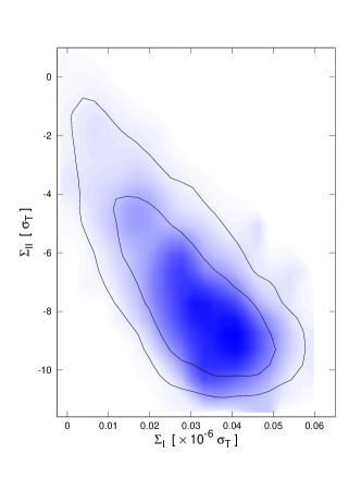
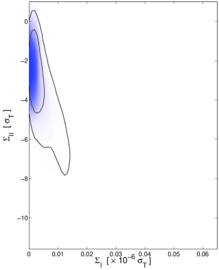
Figure 2: Contour confidence intervals for $\Sigma_{I}$ vs $\Sigma_{II}$ at $68\%$ and $95\%$ c.l. The shading shows the mean likelihood of the samples. Left panel: Considering Set I of observations only. Right panel: Considering Set I and SDSS DR7 LRG observations.

Instead of using the proton mass as the scale in the interactions, we can use an arbitrary associated mass to the dark fluid “particles”, $m_{d}$. We obtain the following constraints at 0.68 c.l. on the ratio $\Sigma/m_{d}$ (we use $c=3\times 10^{10}\rm{cm/s}$):

For the case in which we consider both interactions (Model A)

$$0.21\times 10^{-22}<\frac{\Sigma_{I}}{m_{d}}<1.17\times 10^{-22}\,\,\frac{\rm{cm}^{3}/\rm{s}}{\rm{GeV}/c^{2}}$$ (36)

and

$$-0.96\times 10^{-13}<\frac{\Sigma_{II}}{m_{d}}<-0.35\times 10^{-13}\,\,\frac{\rm{cm}^{3}/\rm{s}}{\rm{GeV}/c^{2}}.$$ (37)

While for Model B,

$$0.10\times 10^{-22}<\frac{\Sigma_{I}}{m_{d}}<0.29\times 10^{-22}\,\,\frac{\rm{cm}^{3}/\rm{s}}{\rm{GeV}/c^{2}}.$$ (38)

Finally, in Figure 3 we show the plots of the angular and matter power spectrums using the best fits values obtained by the MCMC fitting procedure and shown in Table 1.

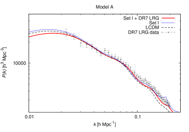
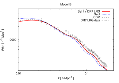
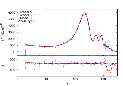
Figure 3: Matter power spectrums for Model A and Model B at redshift $z=0$ and CMB power spectrum for the three models. The parameter values are taken from Table 1.

Note that we have not considered the effect that interactions $I$ and $II$ could have on big bang nucleosynthesis. This is because our phenomenological model only includes the thermalized cross sections $\Sigma_{I}$ and $\Sigma_{II}$ of elastic collisions, whose strengths are at least 9 orders of magnitude weaker than the Thomson scattering at this epoch, and more important, the interactions do not annihilate baryons and, therefore, maintain the baryon-to-photon ratio unaltered. Accordingly, we expect the effect over this process to be quite weak.

3 Non-standard scalar field unification

We now turn to another theoretical scheme that pursues to unify the dark fluids, and it is through a scalar field. There has been works trying to unify dark matter, dark energy, and inflation using scalar fields. In the work in ref. Liddle and Urena-Lopez (2006), where a single scalar field with quadratic potential is used to produce the three phenomena, the inflation phase is driven by the potential as in the usual chaotic inflation scenario. An incomplete reheating phase leaves enough energy in the field for it to oscillate around the minimum of the potential and behave as dark matter Magana and Matos (2012), while a constant term in the potential allows it to reproduce dark energy. However, as mentioned in the Introduction, a fine tuning of the parameters is necessary to accommodate the proper dark matter content.

Other works have used a generalized version of the scalar field Lagrangian in order to accomplish the unification. There the Lagrangian has the form

$$\mathcal{L}=\mathcal{L}(X,\phi),$$ (39)

where the $X=-\frac{1}{2}\phi_{,\mu}\phi^{,\mu}$ is the usual kinetic term, and the Lagrangian is a general function of it and the scalar field $\phi$. This type of scalar fields have been used to model inflation Armendariz-Picon et al. (1999), dark energy Chiba et al. (2000), and also to unify dark energy and dark matter Chimento (2004); Scherrer (2004); Bertacca et al. (2010). Combining one Lagrangian proposed in Chimento (2004) with an appropriate potential term it is possible to obtain a unification of inflation, with dark energy and dark matter as it was made in Bose and Majumdar (2009a, b); De-Santiago and Cervantes-Cota (2011).

3.1 Conditions for Dark Energy and Dark Matter unification

A general Lagrangian of the form of equation (39) has an associated energy density

$$\rho=2X\mathcal{L}_{,X}-\mathcal{L},$$ (40)

and pressure

$$P=\mathcal{L}.$$ (41)

From that one can obtain the equation of state

$$\omega=\frac{\mathcal{L}}{2X\mathcal{L}_{,X}-\mathcal{L}},$$ (42)

and sound speed $c_{s}^{2}=P_{,X}/\rho_{,X}$ given by Garriga and Mukhanov (1999)

$$c_{s}^{2}=\frac{\mathcal{L}_{,X}}{2X\mathcal{L}_{,XX}+\mathcal{L}_{,X}}\,.$$ (43)

If the Lagrangian is the sum of a constant that accounts for the dark energy and a variable part that accounts for the dark matter $\mathcal{L}=\mathcal{L}_{0}+\mathcal{L}_{(dm)}(X,\phi)$, the conditions on the latter are that $\omega_{dm}\ll c^{2}$ and ${c_{(dm)}}_{s}^{2}\ll c^{2}$, as mentioned in the Introduction. The first condition is in order to have a background evolution similar to that of $\Lambda$CDM and the second one in order to allow for structure formation; however this condition can be violated in some models and still have structure formation Magana and Matos (2012). The conditions on the Lagrangian become

$$\frac{\mathcal{L}_{(dm)}}{X\mathcal{L}_{(dm),X}}\ll 1\,,$$ (44)

and

$$\frac{\mathcal{L}_{(dm),X}}{X\mathcal{L}_{(dm),XX}}\ll 1\,.$$ (45)

These conditions are satisfied by a Lagrangian with a minimum at an $X\neq 0$ and the field close to that minimum, so the standard kinetic term $F=X$ does not fulfill them. From the first condition the value of the dark matter part of the Lagrangian in the minimum should be zero.

In the work by Scherrer Scherrer (2004) the Lagrangian

$$\mathcal{L}=F_{0}+F_{m}(X-X_{0})^{2}$$ (46)

is used, where the first term is a constant that accounts for the dark energy and the second term behaves as dark matter as it satisfies equations (44, 45). It is argued in ref. Giannakis and Hu (2005) that this model changes the transfer function, and it is concluded that in order to account for the $\Lambda$CDM power spectrum the deviation from the minimum $\epsilon\equiv(X-X_{0})/X_{0}$ should be smaller than $10^{-16}$ in the present epoch. Fulfilling this condition guarantees this model to be indistinguishable from cold dark matter perturbation growth.

Let us now consider another model. In a previous work De-Santiago and Cervantes-Cota (2011), we employed a Lagrangian proposed in ref. Chimento (2004) with an extra constant term form Bose and Majumdar (2009a):

$$\mathcal{L}=\frac{1}{(2\alpha-1)}\left[(AX)^{\alpha}-2\alpha\alpha_{0}\sqrt{AX}\right]+M.$$ (47)

Here the effective constant term that accounts for dark energy is

$$\mathcal{L}_{0}=M-\alpha_{0}^{2\alpha/(2\alpha-1)}\,,$$ (48)

and the (dark matter) part that satisfies equations (44, 45)

$$\mathcal{L}_{dm}=\frac{1}{(2\alpha-1)}\left[(AX)^{\alpha}-2\alpha\alpha_{0}\sqrt{AX}\right]+\alpha_{0}^{2\alpha/(2\alpha-1)}.$$ (49)

The conditions for this Lagrangian to satisfy the cosmological constraints were studied first in ref. Bose and Majumdar (2009a) for the $\alpha=1$ case and later in ref. De-Santiago and Cervantes-Cota (2011) for the general case with $n=2\alpha/(2\alpha-1)$ a positive integer. The mathematical advantage of this Lagrangian is that the cosmological evolution of the energy density in a flat Friedmann-Robertson-Walker Universe is reduced to the simple equation

$$\rho=\left[\alpha_{0}+\frac{c_{0}}{a^{3}}\right]^{n}-M\,.$$ (50)

This expression can be split into a dark energy term, a dark matter term and extra terms that are functions of larger powers of the scale factor, as follows

$$\rho_{de} = \alpha_{0}^{n}-M,$$ (51)

$$\rho_{dm} = \frac{nc_{0}\alpha_{0}^{n-1}}{a^{3}},$$ (52)

$$\rho_{extra} = \sum_{k=2}^{n}\binom{n}{k}\alpha_{0}^{n-k}\left(\frac{c_{0}}{a^{3}}\right)^{k}.$$ (53)

The conditions (44) and (45) are fulfilled in this model too, since around the minimum the ”dark matter” Lagrangian, equation (49), behaves as Scherrer’s model, with $F_{m}=\frac{1}{4}A^{2}\alpha\,\alpha_{0}^{(2\alpha-4)/(2\alpha-1)}$ and $F_{0}=-\rho_{de}$, see equation (51), where we already added the constant $M$.

In order to have $\rho_{extra}$ negligible during the known evolution of the Universe to avoid spoiling the standard cosmic dynamics at least from nucleosynthesis to today, one is forced to demand the following condition

$$M\gg\rho_{de0}\left[\frac{z_{\rm nuc}^{3n-4}}{(3n)^{n}}\frac{\rho_{de0}}{\rho_{r0}}\right]^{1/(n-1)},$$ (54)

in other words, $M$ has to be more than $10^{10}$ times bigger than the magnitude of the dark energy today but at the same time, from equation (51), it has to cancel almost exactly with $\alpha_{0}^{n}$ to yield the correct value of dark energy. Of course, this is a fine tuning of the model.

In the same way as in the Scherrer’s model the field has to be close to the minimum, in order to have a correct transfer function. The condition given by equation (54) can be used to obtain a bound for the deviation $\epsilon=(X-X_{0})/X_{0}$ as

$$\epsilon\ll(z+1)^{3}2(n-1)(3n)^{1/(n-1)}10^{(-30n+36)/(n-1)}.$$ (55)

which implies, for example, for $n=2$ that the value for $\epsilon$ today is smaller than $10^{-23}$ satisfying the condition obtained from the transfer function in which $\epsilon<10^{-16}$, see figure 4.

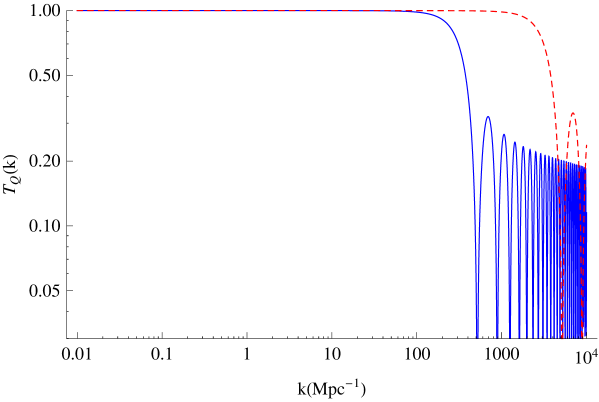
Figure 4: Deviation from the CDM transfer function for the cases $n=2$ (blue, continuos line) and $n=3$ (red, dashed line). The modification becomes significant only for small scales where linear theory is no longer valid.

3.2 Inflation

So far the scalar field with Lagrangian given by equation (47) is able to reproduce the phenomena of dark matter and dark energy in the late Universe, and it only depends on the kinetic term $X$. If we add a potential term to the Lagrangian it can account for the energy density during inflation. For this we chose in De-Santiago and Cervantes-Cota (2011) a quadratic potential

$$V(\phi)=\frac{1}{2}m^{2}\phi^{2}\,.$$ (56)

Due to the large energies during inflation the kinetic term gets reduced to only the first term in the expression (47) with $\alpha>0$, and with this simplification we obtain the effective Lagrangian at high energies

$$\mathcal{L}=\frac{1}{(2\alpha-1)}(AX)^{\alpha}-\frac{1}{2}m^{2}\phi^{2}\,,$$ (57)

which has been well studied as a source for inflation Mukhanov and Vikman (2006); Panotopoulos (2007). The slow roll (sr) parameters for this non-canonical case are given by

$$\epsilon_{\rm sr} = \frac{M_{\rm pl}^{2}}{2F_{X}}\left(\frac{V^{\prime}}{V}\right)^{2},$$ (58)

$$\eta_{\rm sr} = \frac{M_{\rm pl}^{2}}{F_{X}^{2}}\frac{V^{\prime\prime}}{V},$$ (59)

where $F$ is the effective kinetic term in the Lagrangian and $F_{X}$ its derivative with respect to $X$. Supposing that a slow roll regime holds during the inflationary epoch, the end of inflation occurs when it is violated, and $\epsilon_{\rm sr}\sim 1$, which can be simplified to

$$\phi_{f}^{2}=\frac{2M_{\rm pl}^{2}}{F_{X}}.$$ (60)

The beginning of inflation, can be calculated assuming 60 e-folds of inflation. Using the slow roll approximation we find that $\phi_{i}=15.5M_{pl}$. The mass parameter $m$ can be computed in terms of the amplitude of perturbations in the CMB as $m=7\times 10^{-6}M_{pl}(n-1)^{1/4}$. With this data and using the fact that $F_{X}\sim 1$, we can compute the values of the slow roll parameters at the beginning of inflation as $\epsilon_{\rm sr(i)}=8.3\times 10^{-3}$ and $\eta_{\rm sr(i)}=8.3\times 10^{-3}$. And the spectral index and tensor to scalar ratio get the values

$$n_{s} = 1-0.3\sqrt{n-1}\,,$$ (61)

$$r = 0.15\sqrt{n-1}\,.$$ (62)

It yields a much redder power spectrum than Harrison-Zel’dovich’s. The current measurement of the spectral index, from WMAP 9 years plus combined data from e-CMB, BAO, and $H_{0}$, is Hinshaw et al. (2012) $n_{s}=0.961\pm 0.008$. To avoid this inconsistency, as the parameter $m$ and $\phi_{i}$ are constrained, the only possibility is to adjust $F_{X}$ at the beginning of inflation, but we have not made this analysis yet.

When considering all constraints for a successful cosmological model, with exception to the reddish spectral index, the parameters have to comply with, for $\alpha=1$,

$$10^{-48}M_{\rm{Pl}}^{2}< \alpha_{0} <10^{-40}M_{\rm{Pl}}^{2}\,,$$

$$m \sim 10^{-6}M_{\rm{Pl}}\,,$$

$$\alpha_{0}^{2}-M \sim 10^{-120}M_{\rm{Pl}}^{4}\,,$$

$$A \sim 1\,.$$ (63)

This would guarantee a cosmological dynamics that emulates that of the $\Lambda$CDM model over the whole expansion’s history and perturbed kinematics. We notice that the energy scale of $\alpha_{0}^{2}$ and $M$ can be between $(10\,{\rm keV})^{4}$ to $(100\,{\rm MeV})^{4}$, but their difference must be very small to achieve the present cosmological constant value.

3.3 Phase space

One may wonder how a transition from inflation to ”matter” dominated happened and then to a dark energy dominated Universe, and how robust to the different initial conditions the system is. To answer this issue we have performed a phase space analysis of the solutions De-Santiago and Cervantes-Cota (2012) and we present an excerpt pointing out some features of the model. In ref. De-Santiago et al. (2013) a study on the general features of the phase space for models with Lagrangian $\mathcal{L}=F(X)-V(\phi)$ is presented. Here however, we will carry out a similar analysis adapted to the particular choice given by (47,56).

For concreteness, let us consider $\alpha=1$. It is straightforward to show that the system of first order autonomous equations becomes:

$$\dot{z} = -\frac{m^{2}\phi}{\sqrt{A}}+\frac{\sqrt{3}}{2M_{\rm{Pl}}}\left(-\sqrt{2}z+2\alpha_{0}{\rm sign}(z)\right)\sqrt{z^{2}+m^{2}\phi^{2}-2M}\,,$$ (64)

$$\dot{\phi} = \frac{z}{\sqrt{A}}\,.$$ (65)

With the equation of state of the field $p_{\phi}/\rho_{\phi}$ written in terms of these variables as

$$\omega_{\phi}=\frac{2M+z^{2}-\sqrt{8}\alpha_{0}|z|-m^{2}\phi^{2}}{-2M+z^{2}+m^{2}\phi^{2}}\,.$$ (66)

The system doesn’t have any critical points, but the system can be solved numerically to obtain its phase space, shown in Fig. 5. There we have plotted in dotted (red) lines those of constant equation of state, the horizontal lines corresponding to $\omega_{\phi}=-1$ and diagonal lines to $\omega_{\phi}=0$. As can be seen the sector of initial conditions with big negative $\phi$ values and positive $z$ values evolves towards a solution with equation of state near $-1$ which in the phase space corresponds to the left horizontal branch. This in the unification models is interpreted as the initial period of inflation in which the equation of state of the solution gets close to $-1$.

This solution later crosses the lines corresponding to a equation of state equal to 0 (diagonal lines) that in the unification models correspond to the matter domination epoch. The time that the system stays in the regime of $\omega_{\phi}\sim 0$ has to be long in order to mimic dark matter. This time will depend on the value of the parameters (63) in the Lagrangian, and the parameters can be adjusted in accordance to equation (63) in order to obtain this behaviour from a redshift of order $10^{10}$ up until a recent time when the transition to $\omega_{\phi}<0$ has to occur. Finally, the solution evolves towards a second period of $\omega_{\phi}$ close to $-1$, that in the phase space corresponds to the right horizontal branch. The whole behaviour occurs also for solutions beginning with big positive values of $\phi$ and negative values of $z$, in which solutions go from positive to negative values in $\phi$ and live in the $z<0$ part of the phase space, as can be seen in Fig. 5.

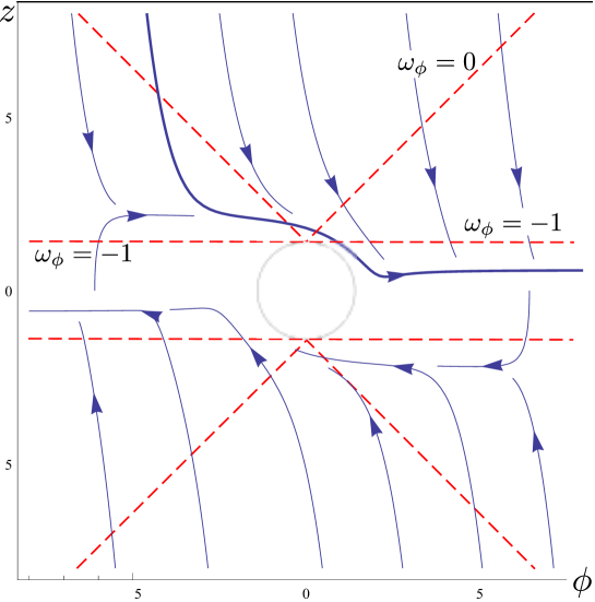
Figure 5: Phase space for the model, the continuous (blue) lines correspond to the evolution of the system. The dotted (red) lines correspond to lines of constant equation of state, both horizontal lines corresponding to $\omega_{\phi}=-1$ and the four $45^{\circ}$ segments correspond to $\omega_{\phi}=0$. A typical solution represented by the thick line approaches first to $\omega_{\phi}\sim-1$ (inflation), then passes through $\omega_{\phi}\sim 0$ emulating dark matter and finally comes back to $\omega_{\phi}\sim-1$ at late times as dark energy.

We conclude that an important sector of the possible initial conditions can yield the expected behavior needed to unify the phenomena of dark matter, dark energy, and inflation with a single, albeit complicated, scalar field.

4 Conclusions

The standard model of cosmology is built with standard particle physics and its interactions, and in addition, one has dark matter and dark energy. On the other hand, an inflationary dynamics is also necessary and it demands a ”dark” component, usually associated to a scalar field that dominated the dynamics and kinematics in the very early Universe. These three dark components are independent from each other since, at least for historical reasons, they were invented to solve different cosmological/astrophysical problems. However, there are many models that aim to unify the dark components of the Universe, all three or in pairs. In the present work, we have updated and tested further two different unification approaches: the dark fluid and an $F(X)$ scalar field.

The dark fluid is constructed to have exactly the same properties as both dark matter and dark energy. Thus, with a single fluid we successfully achieve to reproduce exactly the same dynamics of the $\Lambda$CDM standard model of cosmology. Given the dark degeneracy, there is no way to distinguish, through dynamical or kinematical computations, between the dark fluid and the dark components of the $\Lambda$CDM model. Our proposal implies that dark matter and dark energy do not separately exist, but they constitute a single fluid. We have not analyzed what the possible real candidates for the dark fluid are, but speculating, it could be a cold dark matter particle with an intrinsic (remanent?) small pressure. The dark fluid could also be a collection of barotropic fluids that comply with an effective null sound speed propagation, and again with an associated small pressure. On the other hand, if we add baryonic interactions to the dark fluid, one breaks the degeneracy with $\Lambda$CDM and one can compute the constraints imposed from recent cosmological probes, as we have done in this work.

A triple unification of dark matter, dark energy, and inflation can be carried out by using a particular $F(X)$ Lagrangian and a typical potential term. The first term is necessary to emulate the dark matter behavior in the cosmological evolution. Although we used a very particular model for this aim, we remarked that a cosmological dark matter behavior is achieved with a $F(X)$ scalar field that has a minimum (with $X_{0}\neq 0$) and it stays near to it, and thus it complies with the conditions given by equations (44) and (45), that is, being a ”fluid” with small pressure and speed of sound. The inflationary part is achieved through any standard potential, associated to the scalar field, but some corrections apply stemming from the non-standard kinetic part. In our particular case, this leads to the prediction of a more reddish than measured spectrum of the primordial seeds for perturbations. Ways to change this last conclusion are to be worked out yet. Finally, dark energy is put by hand, but not exactly as in the $\Lambda$CDM model, here a different magnitude for the ”cosmological constant” is needed to be subtracted from a remaining constant of the dark matter part of the Lagrangian. Yet, both constants have to cancel out in a fine tuning way to yield the correct dark energy dynamics.

References

- Cervantes-Cota and Smoot (2011) J. L. Cervantes-Cota, and G. Smoot, AIP Conf.Proc. 1396, 28–52 (2011), 1107.1789.
- Chimento et al. (2003) L. P. Chimento, A. S. Jakubi, D. Pavón, and W. Zimdahl, Phys. Rev. D 67, 083513 (2003), URL http://link.aps.org/doi/10.1103/PhysRevD.67.083513.
- Copeland et al. (2006) E. J. Copeland, M. Sami, and S. Tsujikawa, Int.J.Mod.Phys. D15, 1753–1936 (2006), hep-th/0603057.
- Bertacca et al. (2010) D. Bertacca, N. Bartolo, and S. Matarrese, Adv.Astron. 2010, 904379 (2010), 1008.0614.
- Turner (1983) M. S. Turner, Phys.Rev. D28, 1243 (1983).
- Kofman et al. (1997) L. Kofman, A. D. Linde, and A. A. Starobinsky, Phys. Rev. D56, 3258–3295 (1997), hep-ph/9704452.
- Liddle and Urena-Lopez (2006) A. R. Liddle, and L. A. Urena-Lopez, Phys.Rev.Lett. 97, 161301 (2006), astro-ph/0605205.
- Hinshaw et al. (2012) G. Hinshaw, D. Larson, E. Komatsu, D. Spergel, C. Bennett, et al. (2012), 1212.5226.
- Busca et al. (2012) N. G. Busca, et al. (2012), 1211.2616.
- Aviles and Cervantes-Cota (2011a) A. Aviles, and J. L. Cervantes-Cota, Phys.Rev. D84, 083515 (2011a), 1108.2457.
- Luongo and Quevedo (2011) O. Luongo, and H. Quevedo (2011), 1104.4758.
- Balbi et al. (2007) A. Balbi, M. Bruni, and C. Quercellini, Phys.Rev. D76, 103519 (2007), astro-ph/0702423.
- Xu et al. (2012) L. Xu, Y. Wang, and H. Noh, Phys.Rev. D85, 043003 (2012), 1112.3701.
- Caplar and Stefancic (2013) N. Caplar, and H. Stefancic, Phys.Rev. D87, 023510 (2013), 1208.0449.
- Aviles et al. (2012) A. Aviles, A. Bastarrachea-Almodovar, L. Campuzano, and H. Quevedo, Phys.Rev. D86, 063508 (2012), 1203.4637.
- Kunz (2009) M. Kunz, Phys.Rev. D80, 123001 (2009), astro-ph/0702615.
- Ma and Bertschinger (1995) C.-P. Ma, and E. Bertschinger, Astrophys.J. 455, 7–25 (1995), astro-ph/9506072.
- Bardeen (1980) J. M. Bardeen, Phys.Rev. D22, 1882–1905 (1980).
- Khoury and Weltman (2004a) J. Khoury, and A. Weltman, Phys.Rev.Lett. 93, 171104 (2004a), astro-ph/0309300.
- Khoury and Weltman (2004b) J. Khoury, and A. Weltman, Phys.Rev. D69, 044026 (2004b), astro-ph/0309411.
- Brans and Dicke (1961) C. Brans, and R. Dicke, Phys.Rev. 124, 925–935 (1961).
- Sami and Padmanabhan (2003) M. Sami, and T. Padmanabhan, Phys.Rev. D67, 083509 (2003), hep-th/0212317.
- Aviles and Cervantes-Cota (2011b) A. Aviles, and J. L. Cervantes-Cota, Phys.Rev. D83, 023510 (2011b), 1012.3203.
- Hui and Nicolis (2010) L. Hui, and A. Nicolis, Phys.Rev.Lett. 105, 231101 (2010), 1009.2520.
- Spergel and Steinhardt (2000) D. N. Spergel, and P. J. Steinhardt, Phys.Rev.Lett. 84, 3760–3763 (2000), astro-ph/9909386.
- Wandelt et al. (2000) B. D. Wandelt, R. Dave, G. R. Farrar, P. C. McGuire, D. N. Spergel, et al. pp. 263–274 (2000), astro-ph/0006344.
- Lewis and Bridle (2002) A. Lewis, and S. Bridle, Phys.Rev. D66, 103511 (2002), astro-ph/0205436.
- Larson et al. (2011) D. Larson, J. Dunkley, G. Hinshaw, E. Komatsu, M. Nolta, et al., Astrophys.J.Suppl. 192, 16 (2011), 1001.4635.
- Riess et al. (2009) A. G. Riess, L. Macri, S. Casertano, M. Sosey, H. Lampeitl, et al., Astrophys.J. 699, 539–563 (2009), 0905.0695.
- Amanullah et al. (2010) R. Amanullah, C. Lidman, D. Rubin, G. Aldering, P. Astier, et al., Astrophys.J. 716, 712–738 (2010), 1004.1711.
- Reid et al. (2010) B. A. Reid, W. J. Percival, D. J. Eisenstein, L. Verde, D. N. Spergel, et al., Mon.Not.Roy.Astron.Soc. 404, 60–85 (2010), 0907.1659.
- Magana and Matos (2012) J. Magana, and T. Matos, J.Phys.Conf.Ser. 378, 012012 (2012), 1201.6107.
- Armendariz-Picon et al. (1999) C. Armendariz-Picon, T. Damour, and V. F. Mukhanov, Phys. Lett. B458, 209–218 (1999), hep-th/9904075.
- Chiba et al. (2000) T. Chiba, T. Okabe, and M. Yamaguchi, Phys. Rev. D62, 023511 (2000), astro-ph/9912463.
- Chimento (2004) L. P. Chimento, Phys.Rev. D69, 123517 (2004), astro-ph/0311613.
- Scherrer (2004) R. J. Scherrer, Phys. Rev. Lett. 93, 011301 (2004), astro-ph/0402316.
- Bose and Majumdar (2009a) N. Bose, and A. S. Majumdar, Phys. Rev. D79, 103517 (2009a), 0812.4131.
- Bose and Majumdar (2009b) N. Bose, and A. Majumdar, Phys.Rev. D80, 103508 (2009b), 0907.2330.
- De-Santiago and Cervantes-Cota (2011) J. De-Santiago, and J. L. Cervantes-Cota, Phys.Rev. D83, 063502 (2011), 1102.1777.
- Garriga and Mukhanov (1999) J. Garriga, and V. F. Mukhanov, Phys.Lett. B458, 219–225 (1999), hep-th/9904176.
- Giannakis and Hu (2005) D. Giannakis, and W. Hu, Phys.Rev. D72, 063502 (2005), astro-ph/0501423.
- Mukhanov and Vikman (2006) V. F. Mukhanov, and A. Vikman, JCAP 0602, 004 (2006), astro-ph/0512066.
- Panotopoulos (2007) G. Panotopoulos, Phys.Rev. D76, 127302 (2007), 0712.1713.
- De-Santiago and Cervantes-Cota (2012) J. De-Santiago, and J. L. Cervantes-Cota, AIP Conf.Proc. 1473, 59–67 (2012), 1206.2036.
- De-Santiago et al. (2013) J. De-Santiago, J. L. Cervantes-Cota, and D. Wands, Phys.Rev. D87, 023502 (2013), 1204.3631.