The VIMOS Public Extragalactic Redshift Survey (VIPERS)

We present in this paper the general real- and redshift-space clustering properties of galaxies as measured in the first data release of the VIPERS survey. VIPERS is a large redshift survey designed to probe in detail the distant Universe and its large-scale structure at $0.5<z<1.2$. We describe in this analysis the global properties of the sample and discuss the survey completeness and associated corrections. This sample allows us to measure the galaxy clustering with an unprecedented accuracy at these redshifts. From the redshift-space distortions observed in the galaxy clustering pattern we provide a first measurement of the growth rate of structure at $z=0.8$: $f\sigma_{8}=0.47\pm 0.08$. This is completely consistent with the predictions of standard cosmological models based on Einstein gravity, although this measurement alone does not discriminate between different gravity models.

1 Introduction

Over the past decades galaxy redshift surveys have provided a wealth of information on the inhomogeneous universe, mapping the late-time development of the small metric fluctuations that existed at early times, and whose early properties can be viewed in the cosmic microwave background (CMB). The growth of structure during this intervening period is sensitive both to the type and amount of dark matter, and also to the theory of gravity, so there is a strong motivation to make precise measurements of the rate of growth of cosmological structure (e.g. Jain & Khoury 2010).

Of course, galaxy surveys do not image the mass fluctuations directly, unlike gravitational lensing. But the visible light distribution does have some advantages as a cosmological tool in comparison with lensing. The number density of galaxies is sufficiently high that the density field of luminous matter can be measured with a finer spatial resolution, probing interesting nonlinear features of the clustering pattern with good signal-to-noise. The price to be paid for this is that the complicated biasing relation between visible and dark matter has to be confronted; but this is a positive factor in some ways, since understanding galaxy formation is one of the main questions in cosmology. Redshift surveys provide the key information needed to meet this challenge: global properties of the galaxy population and their variation with environment and with epoch.

The final advantage of redshift surveys is that the radial information depends on cosmological expansion and is corrupted by peculiar velocities. Although the lack of a simple method to recover true distances can be frustrating at times, it has come to be appreciated that this complication is in fact a good thing. The peculiar velocities induce an anisotropy in the apparent clustering, from which the properties of the peculiar velocities can be inferred much more precisely than in any attempt to measure them directly using distance estimators. The reason peculiar velocities are important is that they are related to the underlying linear fractional density perturbation $\delta$ via the continuity equation: $\dot{\delta}=-{\mathbf{\nabla\cdot u}}$, where $\@vec{u}$ is the peculiar velocity field. This can be expressed more conveniently in terms of the dimensionless scale factor, $a(t)$, and the Hubble parameter, $H(t)$, as

$${\@vec{\nabla\cdot u}}=-Hf\delta;\quad f\equiv{d\ln\delta\over d\ln a}.$$ (1)

The growth rate can be approximated in most models by $f(a)\simeq\Omega_{m}(a)^{\gamma}$, where $\gamma\simeq 0.545$ in standard $\Lambda$-dominated models, but where models of non-standard gravity display a growth rate in which the effective value of $\gamma$ can differ by $30\%$ (Linder & Cahn 2007).

The possibility of using the redshift-space distortion signature as a probe of the growth rate of density fluctuations, together with that of using the Baryonic Acoustic Oscillations (BAO) as a standard ruler to measure the expansion history, is one of the main reasons behind the recent burst of activity in galaxy redshift surveys. The first paper to emphasise this application as a test of gravity theories was the analysis of the VVDS survey by Guzzo et al. (2008), and subsequent work especially by the SDSS LRG (Samushia et al. 2012), WiggleZ (Blake et al. 2012; Contreras et al. 2013), 6dFGS (Beutler et al. 2012) and BOSS (Reid et al. 2012) surveys has exploited this method to make measurements of the growth rate at $z<1$.

Surveys such as SDSS LRG, WiggleZ, or BOSS are characterized by a large volume ($0.5-2\,h^{-3}{\rm Gpc}^{3}$), and a relatively sparse galaxy population with number density of about $10^{-4}\,h^{3}{\rm Mpc}^{-3}$. Statistical errors are in this case minimized thanks to the large volume probed, at the expenses of selecting a very specific galaxy population (e.g. blue star forming or very massive galaxies), often with a complex selection function. The goal of the VIMOS Public Extragalactic Redshift Survey (VIPERS, http://vipers.inaf.it), has been that of constructing a survey with broader science goals and properties comparable to local general-purpose surveys such as the 2dFGRS. The adopted strategy has been to optimise the features of the ESO VLT multi-object spectrograph VIMOS in order to measure about $\sim 400$ spectra at $I_{AB}<22.5$ over an area of $\sim 200$ square arcmin, in a single exposure of less than $1$ hour. The survey is being performed as a “Large Programme” within the ESO general user framework and aims at measuring redshifts for about $10^{5}$ galaxies at $0.5<z<1.2$.

The prime goal of VIPERS is an accurate measurement of the growth rate of large-scale structure at redshift around unity. The survey should enable us in particular to use of techniques aimed at improving the precision on the growth rate (McDonald & Seljak 2009) thanks to its high galaxies sampling of about $10^{-2}\,h^{3}{\rm Mpc}^{-3}$. In general, VIPERS is intended to provide robust and precise measurements of the properties of the galaxy population at an epoch when the Universe was about half its current age, representing one of the largest spectroscopic surveys of galaxies ever conducted at these redshifts. Examples can be found in the parallel papers that are part of the first science release (Marulli et al. 2013; Malek et al. 2013; Davidzon et al. 2013).

This paper presents the initial analysis of the real-space galaxy clustering and redshift-space distortions in VIPERS, together with the resulting implications for the growth rate. The data are described in Section 2; Section 3 describes the survey selection effects; Section 4 describes our methods for estimating clustering, which are tested on simulations in Section 5; Section 6 presents the real-space clustering results; Section 7 gives the redshift-space distortions results, and Section 8 summarises our results and concludes.

Throughout this analysis, if not specified otherwise, we assume a fiducial $\Lambda{\rm CDM}$ cosmological model with $(\Omega_{m},\Omega_{k},w,\sigma_{8},n_{s})=(0.25,0,-1,0.8,0.95)$ and a Hubble constant of $H_{0}=100\leavevmode\nobreak\ h\leavevmode\nobreak\ \rm{km\leavevmode\nobreak\ s^{-1}\leavevmode\nobreak\ Mpc^{-1}}$.

2 Data

The VIPERS galaxy target sample is selected from the optical photometric catalogues of the Canada-France-Hawaii Telescope Legacy Survey Wide (CFHTLS-Wide, Goranova et al. 2009). VIPERS covers $24$ deg² on the sky, divided over two areas within the W1 and W4 CFHTLS fields. Galaxies are selected to a limit of $i^{\prime}_{AB}<22.5$, applying a simple and robust $gri$ colour pre-selection to efficiently remove galaxies at $z<0.5$. Coupled with a highly optimized observing strategy (Scodeggio et al. 2009), this allows us to double the galaxy sampling rate in the redshift range of interest, with respect to a pure magnitude-limited sample. At the same time, the area and depth of the survey result in a relatively large volume, $5\times 10^{7}\,h^{-3}\leavevmode\nobreak\ \rm{Mpc^{3}}$, analogous to that of the Two Degree Field Galaxy Redshift Survey (2dFGRS) at $z\simeq 0.1$ (Colless et al. 2001, 2003). Such a combination of sampling rate and depth is unique amongst current redshift surveys at $z>0.5$. VIPERS spectra are collected with the VIMOS multi-object spectrograph (Le Fèvre et al. 2003) at moderate resolution ($R=210$) using the LR Red grism, providing a wavelength coverage of 5500-9500$\rm{\AA}$ and a typical radial velocity error of $\sigma_{v}=175(1+z)$$\,{\rm km\,s^{-1}}$. The full VIPERS area of $24$ deg² will be covered through a mosaic of 288 VIMOS pointings (192 in the W1 area, and 96 in the W4 area). A discussion of the survey data reduction and management infrastructure is presented in Garilli et al. (2012). An early subset of the spectra used here is analysed and classified through a Principal Component Analysis (PCA) in Marchetti et al. (2013). A complete description of the survey construction, from the definition of the target sample to the actual spectra and redshift measurements, is given in the parallel survey description paper (Guzzo et al. 2013).

The data set used in this and the other papers of the early science release, will represent the VIPERS Public Data Release 1 (PDR-1) catalogue. It will be publicly available in the fall of 2013. This catalogue includes $55358$ redshifts ($27935$ in W1 and $27423$ in W4) and corresponds to the reduced data frozen in the VIPERS database at the end of the 2011/2012 observing campaign; this represents $64\%$ of the final survey in terms of covered area. A quality flag has been assigned to each object in the process of determining their redshift from the spectrum, which quantifies the reliability of the measured redshifts. In this analysis, we use only galaxies with flags 2 to 9 inclusive, corresponding to a sample with a redshift confirmation rate of $98\%$. The redshift confirmation rate and redshift accuracy have been estimated using repeated spectroscopic observations in the VIPERS fields (see Guzzo et al. 2013, for details). The catalogue, which we will refer to just as the VIPERS sample in the following, corresponds to a sub-sample of $45871$ galaxies with reliable redshift measurements.

The redshift distribution of the sample is presented in Fig. 1. We can see in this figure that the survey colour selection allows an efficient removal of galaxies below $z=0.5$. It is important to notice that the colour selection does not introduce a sharp cut in redshift but a redshift window function which has a smooth transition from zero to one in the redshift range $0.4<z<0.6$, with respect to the full population of $i^{\prime}<22.5$ galaxies. This effect on the radial selection of the survey, which we refer to as the Colour Sampling Rate (${CSR}$) in the following, is only present below $z=0.6$. Above this redshift, the colour selection has no impact on the redshift selection and the sample becomes purely magnitude-limited at $i^{\prime}<22.5$ (Guzzo et al. 2013). If we weight the raw redshift distribution by the global survey completeness function described in the next sections, one obtains the $N(z)$ represented by the empty histogram in Fig. 1. For convenience, we scaled down the corrected $N(z)$ by $40\%$, the average effective survey sampling rate, to aid the comparison between the shapes of the two distributions. The difference in shape between these two $N(z)$ shows the effect of incompleteness in the survey, which is only significant at about $z>0.9$ (see also Davidzon et al. 2013).

Figure 1: Redshift distribution of the combined W1+W4 galaxy sample when including only reliable redshifts (filled histogram) and that corrected for the full survey completeness (empty histogram) scaled down by 40% (see text). The curve shows the best-fitting template redshift distribution given by Eq. 2 applied to the uncorrected observed distribution.

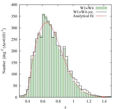
The observed redshift distribution in the sample can be well described by a function of the form

$$N(z)=A\left(\frac{z}{z_{0}}\right)^{\alpha}\exp\left(-\left(\frac{z}{z_{0}}\right)^{\beta}\right){CSR}(z),$$ (2)

in units of $\rm{deg}^{-2}\cdot(\Delta z=0.03)^{-1}$ and where $(A,z_{0},\alpha,\beta)=(3.103,0.191,8.603,1.448)$. The ${CSR}$ is the incompleteness introduced by the VIPERS colour selection. It is primarily a function of redshift and can be estimated from the ratio between the number of galaxies with $i^{\prime}<22.5$ satisfying the VIPERS colour selection and the total number of galaxies with $i^{\prime}<22.5$ as a function of redshift. We calibrated this function using the VLT-VIMOS Deep Survey Wide spectroscopic sample (VVDS-Wide, Garilli et al. 2008) which has a CFHTLS-based photometric coverage and depth that is similar to that of VIPERS, but which is free from any colour selection (see Guzzo et al. 2013, for details). The ${CSR}$ is well described by a function of the form

$${CSR}(z)=\left[\frac{1}{2}-\frac{{\rm erf}\left(b(z_{t}-z)\right)}{2}\right],$$ (3)

with $(b,z_{t})=(17.465,0.424)$.

The fitting of $N(z)$ is important in measuring galaxy clustering: the form of the mean redshift distribution must be followed accurately, but features from large-scale structure must not be allowed to bias the result. We discuss this issue in detail in Section 5.

3 Angular completeness

3.1 Slit assignment and footprint

To obtain a sample of several square degrees with VIMOS, one needs to perform a series of individual observations or pointings. The VIPERS strategy consists in covering the survey area with only one pass. This has been done in order to maximise the volume probed. The survey strategy and the fact that the VIMOS field-of-view is composed of four quadrants delimited by an empty cross, create a particular footprint on the sky which is reproduced in Figs 4 and 5. In each pointing, slits are assigned to a number of potential targets which meet the survey selection criteria. This is shown in Fig. 2, which illustrates how the slits are positioned in the pointing W1P082. Given the surface density of the targeted population, the multiplex capability of VIMOS, and the survey strategy, a fraction of about $45\%$ of the parent photometric sample can be assigned to slits. We define the fraction of target which have a measured spectrum as the Target Sampling Rate (${TSR}$) and the fraction of observed spectra with reliable redshift measurement as the Spectroscopic Sampling Rate (${SSR}$). The number of slits assigned per pointing is maximized by the SSPOC algorithm (Bottini et al. 2005), but the elongated size of the spectra means that the resulting sampling rate is not uniform inside the quadrants. The dispersion direction of the spectra in VIPERS are aligned with the Dec direction and consequently, the density of spectra along this direction is lower with respect to that along the RA direction. This particular sampling introduces an observed anisotropic distribution of pair separation, which has to be accounted for in order to measure galaxy clustering correctly.

Figure 2: Illustration of the slit assignment in pointing W1P082. The slits are shown in red and associated rectangles represent the typical dispersion of the spectra. All objects meeting the survey selection criteria (potential spectroscopic targets) are represented by black circles.

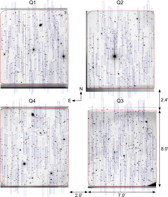
The two empty stripes between the four quadrants in each pointing introduce a particular pattern in the measured correlation functions if not accounted for. We correct for that by applying detailed binary masks of the spectroscopic observations to a random sample of unclustered objects, so that both data and random catalogues contain no objects in these stripes. These masks account for the detailed VIMOS field-of-view geometry as well as for the presence of vignetted areas at the boundaries of the pointings. On top of these spectroscopic masks, we apply a set of photometric masks which discard areas where the parent photometry is affected by defects such as large stellar haloes and where the survey selection is compromised (see Guzzo et al. 2013).

3.2 Small-scale incompleteness

We can characterise the amount of missing small-scale angular pairs induced by the VIPERS spectroscopic strategy, by measuring the angular pair completeness as a function of angular separation. This quantity, defined as the ratio between the number of pairs in the spectroscopic sample and that in the parent photometric sample, can be written in terms of angular two-point correlation functions as (Hawkins et al. 2003)

$$\frac{1}{w^{A}(\theta)}=\frac{1+w_{s}(\theta)}{1+w_{p}(\theta)},$$ (4)

where $w_{s}(\theta)$ and $w_{p}(\theta)$ are respectively the angular correlation function of the spectroscopic and parent samples. This function is shown in Fig. 3. No significant difference is seen between the W1 and W4 fields, as expected. The amount of missing angular pairs is only significant below $\theta=0.03$ deg, which corresponds to a transverse comoving scale of about $1\,h^{-1}\leavevmode\nobreak\ \rm{Mpc}$ at $z=0.8$.

This fraction varies with redshift, although in practice we cannot measure it at different redshifts since we do not have a measured redshift for all galaxies in the parent sample. For this reason we use the global $w^{A}(\theta)$ (averaged over all observed redshifts) to correct for the small-scale angular incompleteness effect. We will show in Section 5 that the level of systematic error introduced by using $w^{A}(\theta)$ instead of $w^{A}(\theta|z)$ is very small, of the order of a few percent. When measuring the angular correlation functions, we include the completeness weights introduced in the following section, in a similar way as for the three-dimensional correlation function estimation.

Figure 3: Completeness fraction of angular galaxy pairs due to the slit-spectroscopy strategy in the W1 and W4 fields for all galaxies at $0.5<z<1.0$. This has been obtained from the parent and spectroscopic sample angular correlation function.

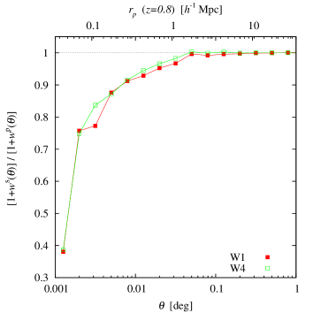
It is important to mention that the small-scale angular incompleteness effect is a general issue for large galaxy redshift surveys, in which one has to deal with the mechanical constraints of multi-object spectrographs and survey strategy. The incompleteness due to slit assignment in VIPERS is to some extent similar to the fibre collision problem in surveys using fibre spectroscopy such as 2dFGRS or SDSS, while the magnitude of the effect is much more severe in our case. Recently, a new method has been developed to accurately correct for fibre collision (Guo et al. 2012). Although this method is quite general, it is not applicable here. The exclusion between spectroscopically observed objects in VIPERS is essentially uni-directional, meaning that not all close pairs are excluded. Therefore calculations such as that shown in Fig. 4 are possible from the set of one-pass observations, whereas the correction scheme of (Guo et al. 2012) can only be used for SDSS where overlapping observations are included. Thus we need to revise the correction methods developed for such surveys to apply them to VIPERS.

3.3 Large-scale incompleteneness

Figure 4: Variations of the target success rate (${TSR}$) with quadrants. The ${TSR}$ quantifies our ability of obtaining spectra from the potential targets meeting the survey selection in the parent photometric sample. The quadrants filled in black correspond to failed observations where no spectroscopy has been taken.

Figure 5: Variations of the spectroscopic success rate (${SSR}$) with quadrants. The ${SSR}$ quantifies our ability of determining galaxy redshifts from observed spectra. The quadrants filled in black correspond to failed observations where no spectroscopy has been taken.

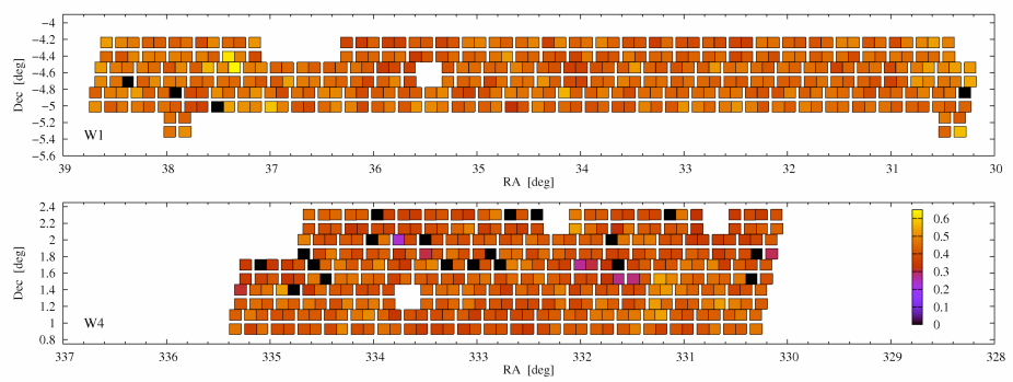
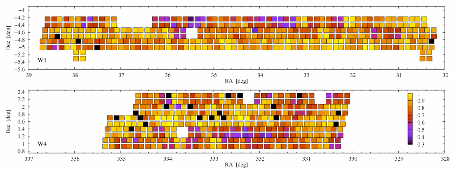
In addition to the non-uniform sampling inside the pointings, the survey has variations of completeness from quadrant to quadrant. This incompleteness is the combined effect of the ${TSR}$ and ${SSR}$. The latter, which characterises our ability of determining a redshift from a galaxy spectrum, is determined empirically as the ratio between the number of reliable redshifts and the total number of observed spectra. The ${TSR}$ and ${SSR}$ in each quadrant are shown in in Figs 4 and 5. From these figures one can see clearly that both ${TSR}$ and ${SSR}$ functions vary according to the position on the sky, although the ${SSR}$ tends to have stronger variations. The variations of ${TSR}$ reflect the changes in angular galaxy density in the parent catalogue. Indeed, because of the finite maximum number of slits that can be assigned and the fact that each quadrant has a different number of potential targets, the less dense quadrants tend to be better sampled than the denser ones. On the other hand, variations in observational conditions from pointing to pointing induce changes in ${SSR}$. These different observational conditions translate into variations of the signal-to-noise of the measured spectra and so in our ability of extracting a redshift measurement from them. These effects are taken into account in the clustering estimation by weighting each galaxy according to the reciprocal of the ${TSR}$ and ${SSR}$.

4 Clustering estimation

We characterise the galaxy clustering in the VIPERS sample by measuring the two-point statistics of the spatial distribution of galaxies in configuration space. We estimate the two-point correlation function $\xi(r)$ using the Landy & Szalay (1993) estimator

$$\xi(r)=\frac{GG(r)-2GR(r)+RR(r)}{RR(r)},$$ (5)

where $GG(r)$, $GR(r)$, and $RR(r)$ are respectively the normalized galaxy-galaxy, galaxy-random, and random-random number of pairs with separation inside $[r-\Delta r/2,r+\Delta r/2]$. Note that here $r$ is a general three-dimensional galaxy separation, not specifically the real-space separation. This estimator minimises the estimation variance and circumvent discreteness and finite volume effects (Landy & Szalay 1993; Hamilton 1993). A random catalogue must be constructed in this estimator, whose aim is to accurately estimate the number density of objects in the sample. It must be an unclustered population of objects with the same radial and angular selection functions as the data. In this analysis, we use random samples with 20 times more objects than in the data to minimise the shot noise contribution in the estimated correlation functions.

VIPERS has a complex angular selection function which has to be taken into account carefully when estimating the correlation function. For this, we weight each galaxy by the survey completeness weight, as well as each pair by the angular pair weights described in the previous section (Eq. 4). The survey completeness weights correspond to the inverse of the effective sampling rate ${ESR}$ in each quadrant $Q$, defined as

$$w(Q)=ESR^{-1}(Q)=(SSR(Q)\times TSR(Q))^{-1}.$$ (6)

By applying these weights we effectively up-weight galaxies in the pair counts. It is important to note that here we keep the spatial distribution of the random objects uniform across the survey volume. We recall that survey completeness weights account for the quadrant-to-quadrant variations of the survey completeness described in Section 3.3 but do not correct for the internal quadrant incompleteness. For that we use the angular pair weights $w^{A}(\theta)$ which are applied to the GG pair counts. In principle the ${ESR}$ is also a function of redshift and galaxy type (see Davidzon et al. 2013). However, given the statistics of the sample it is impossible to measure the additional dependence of this function on redshift and galaxy properties. Therefore, we decided to only account for its quadrant-to-quadrant variations. We discuss the accuracy of this approximation in Section 5.

Additional biases can arise if the radial selection function exhibits strong variations with redshift. The effect is particularly significant for magnitude-limited catalogues covering a large range of redshifts and in which the radial selection function rapidly drops at high redshift. In that case, the pair counts is dominated by nearby, more numerous objects: distant objects, although probing larger volumes, will have less weight. To account for this we use the minimum variance estimator of Davis & Huchra (1982) for which the galaxy counts are essentially weighted by the inverse of the volume probed by each galaxy. This weighting scheme, usually referred as the $J_{3}$ weighting, is defined as (Hamilton 1993)

$$w^{J_{3}}(z,s)=\frac{1}{1+\bar{n}(z)4\pi J_{3}(s)}\,,$$ (7)

where $z$ is the redshift of the object, $s$ is the redshift-space pair separation, $\bar{n}(r)$ the galaxy number density at $z$ and $J_{3}(s)$ is defined as

$$J_{3}(s)=\int_{0}^{s}s^{\prime 2}\xi(s^{\prime})ds^{\prime}.$$ (8)

Each pair is then weighted by,

$$w^{J_{3}}_{ij}=w^{J_{3}}_{i}(z_{i},s_{ij})w^{J_{3}}_{j}(z_{j},s_{ij}).$$ (9)

However, we find that applying $J_{3}$ weighting does not significantly change the amplitude and shape of the correlation function in our sample, and tends to produce noisy correlation functions especially for high-redshift sub-samples. We thus decided not to apply this correction in this analysis.

The final weight assigned to $GG$, $GR$, and $RR$ pairs combine the survey completeness and angular pair weights as

$$GG(r) =\sum_{i=1}^{N_{G}}\sum_{j=i+1}^{N_{G}}w_{i}(Q_{i})w_{j}(Q_{j})w^{A}(\theta_{ij})\Theta_{ij}\left(r\right)$$ (10)

$$GR(r) =\sum_{i=1}^{N_{G}}\sum_{j=1}^{N_{R}}w_{i}(Q_{i})\Theta_{ij}\left(r\right)$$ (11)

$$RR(r) =\sum_{i=1}^{N_{R}}\sum_{j=i+1}^{N_{R}}\Theta_{ij}\left(r\right)\,,$$ (12)

where $\Theta_{ij}(r)$ is equal to unity for $r_{ij}$ in $[r-\Delta r/2,r+\Delta r/2]$ and null otherwise.

We measure correlation functions using both linear and logarithmic binning. We define the separation associated with each bin as the bin centre and as the mean pair separation inside the bin, respectively for the linear and logarithmic binning (Zehavi et al. 2011). The latter definition is more accurate than using the bin centre, in particular at large $r$ when the bin size is large.

The galaxy real-space correlation function $\xi(r)$ is not directly measurable from redshift survey catalogues because of galaxy peculiar velocities that affect redshift measurements. Galaxy peculiar velocities introduce distortions in the galaxy clustering pattern and as a consequence we can only measure redshift-space quantities. We measure the anisotropic redshift-space correlation function $\xi(r_{p},\pi)$ in which the redshift-space galaxy separation vector has been divided in two components, $r_{p}$ and $\pi$, respectively perpendicular and parallel to the line-of-sight (Fisher et al. 1994). This decomposition, which assumes the plane-parallel approximation, allows us to isolate the effect of peculiar velocities as these modify only the component parallel to the line-of-sight. Redshift-space distortions can then be mitigated by integrating $\xi(r_{p},\pi)$ over $\pi$, thus defining the projected correlation function

$$w_{p}(r_{p})=\int^{\pi_{\rm max}}_{-\pi_{\rm max}}\xi(r_{p},\pi)d\pi.$$ (13)

We measure $w_{p}(r_{p})$ using an optimal value of $\pi_{\rm max}=40\,h^{-1}\leavevmode\nobreak\ \rm{Mpc}$, allowing us to reduce the underestimation of the amplitude of $w_{p}(r_{p})$ on large scales and at the same time to avoid including noise from uncorrelated pairs with separations of $\pi>40\,h^{-1}\leavevmode\nobreak\ \rm{Mpc}$. The projected correlation function allows us to measure real-space clustering (but see the later parts of Section 5). To combine the correlation function measurements from the two fields, we measure the mean of one plus the correlation functions in W1 and W4 weighted by the square of the number density, so that the combined correlation function $\xi(r_{p},\pi)$ is obtained from

$$1+\xi(r_{p},\pi)=\frac{n^{2}_{W1}(1+\xi_{W1}(r_{p},\pi))+n^{2}_{W4}(1+\xi_{W4}(r_{p},\pi))}{n^{2}_{W1}+n^{2}_{W4}},$$ (14)

where $n_{W1}$ and $n_{W4}$ are the observed galaxy number densities in the W1 and W4 fields respectively.

5 Tests of the clustering estimation

5.1 Simulation data

To test the robustness of our clustering estimation we make use of a large number of mock galaxy samples, which are designed to be a realistic match to the VIPERS sample. We create two sets of mock samples based on the Halo Occupation Distribution (HOD) technique. These two sets only differ by the input halo catalogue that has been used. In the first set of mocks, we used the haloes extracted from the MultiDark dark matter N-body simulation (Prada et al. 2012). This simulation, which assumes a flat $\Lambda{\rm CDM}$ cosmology with $(\Omega_{m},\leavevmode\nobreak\ \Omega_{\Lambda},\leavevmode\nobreak\ \Omega_{b},\leavevmode\nobreak\ h,\leavevmode\nobreak\ n,\leavevmode\nobreak\ \sigma_{8})=(0.27,\leavevmode\nobreak\ 0.73,\leavevmode\nobreak\ 0.0469,\leavevmode\nobreak\ 0.7,\leavevmode\nobreak\ 0.95,\leavevmode\nobreak\ 0.82)$, covers a volume of $1\,h^{-3}\leavevmode\nobreak\ \rm{Gpc^{3}}$ using $N=2048^{3}$ particles. In the simulation, the haloes have been identified using a friends-of-friends algorithm with a relative linking length of $b=0.17$ times the inter-particle separation (i.e. $0.083\,h^{-1}\leavevmode\nobreak\ \rm{Mpc}$) . The mass limit to which halo catalogues are complete is $10^{11.5}\,h^{-1}\leavevmode\nobreak\ \rm{M_{\odot}}$. Because this limiting mass is too large to host the faintest galaxies observed with VIPERS, we use the method of de la Torre & Peacock (2012) to reconstruct haloes below the resolution limit. This method is based on stochastically resampling the halo number density field using constraints from the conditional halo mass function. For this, one needs to assume the shapes of the halo bias factor and halo mass function at masses below the resolution limit and use the analytical formulae obtained by Tinker et al. (2008, 2010). With this method we are able to populate the simulation with low-mass haloes with a sufficient accuracy to have unbiased galaxy two-point statistics in the simulated catalogues (see de la Torre & Peacock 2012, for details). The minimum reconstructed halo mass we consider for the purpose of creating VIPERS mocks is $10^{10}\,h^{-1}\leavevmode\nobreak\ \rm{M_{\odot}}$.

We then apply to the complete halo catalogues the algorithm presented in Carlson & White (2010) to remap halo positions and velocities in the initial simulation cube onto a cuboid of the same volume but different geometry. This is done to accommodate a maximum number of disjoint VIPERS W1 and W4 fields within the $1\,h^{-3}\leavevmode\nobreak\ \rm{Gpc^{3}}$ volume of the simulation. This process allows us to create 26 and 31 independent lightcones for W1 and W4 respectively over the redshift range $0.4<z<1.3$. The lightcones are built by considering haloes from the different snapshots, disposing them according to their distance from the coordinate origin of the lightcone. The lightcones are then populated with galaxies using the HOD technique. In this process, we populate each halo with galaxies according to its mass, the mean number of galaxies in a halo of a given mass being given by the HOD. It is common usage to differentiate between central and satellite galaxies in haloes. While the former are put at rest at halo centres, the latter are randomly distributed within each halo according to a NFW radial profile. The halo occupation function and its dependence on redshift and luminosity/stellar mass must be precisely chosen in order to obtain mock catalogues with realistic galaxy clustering properties. We calibrated the halo occupation function directly on the VIPERS data. We performed an analytic HOD modelling of the projected correlation function for different samples selected in luminosity and redshift that we will present in Section 6. We obtain from this a series of HOD parameters at different redshifts and for different cuts in $B$-band absolute magnitude, which we then interpolate to obtain a general redshift- and $B$-band absolute magnitude-dependent halo occupation function $\langle N_{\rm gal}(m|z,M_{B})\rangle$. We use the latter function to populate the haloes with galaxies. Finally, we add velocities to the galaxies and measure their redshift-space positions. While the central galaxies are assigned the velocity of their host halo, satellite galaxies have an additional random component for which each Cartesian velocity component is drawn from a Gaussian distribution with a standard deviation that depends on the mass of the host halo. Details about the galaxy mock catalogue construction are given in Appendix A.

The second set of mocks that we built is based on halo catalogues created with the Pinocchio code (Monaco et al. 2002). This code follows the evolution of a set of particles on a regular grid using an ellipsoidal model to compute collapse times and identify dark matter halos, and the Zel’dovich approximation to displace the haloes from their initial position. While the recovery of haloes works well on an object-by-object basis, their positions and velocities on scales below $10\,h^{-1}\leavevmode\nobreak\ \rm{Mpc}$ suffer by the lack of accuracy of the Zel’dovich approximation. The halo positions and velocities obtained with this method are less accurate than those from the N-body simulation, and the halo clustering is generally underestimated on scales below $3\,h^{-1}\leavevmode\nobreak\ \rm{Mpc}$ (e.g. Monaco et al. 2002). However this approach has the advantage of being very fast and can be used to generate a large number of independent halo catalogue realizations. We created $200$ independent halo mock realizations assuming the same cosmology as the MultiDark N-body simulation. The remaining steps in generating galaxy mock samples are similar to those used for the mocks based on the MultiDark simulation. The only difference is that here we do not need to divide each simulation into sub-volumes to generate different lightcones: we can directly create volumes of the size of the lightcones.

The final step in obtaining fully realistic VIPERS mocks is to add the detailed survey selection function. The procedure that we follow is similar to that used in the VVDS and zCOSMOS surveys, which were also based on VIMOS observations (Meneux et al. 2006; Iovino et al. 2010; de la Torre et al. 2011). We start by applying the magnitude cut $i^{\prime}<22.5$ and the effect of the colour selection on the radial distribution of the mocks. The latter is done by depleting the mocks at $z<0.6$ so as to reproduce the ${CSR}$. The mock catalogues that we obtain are then similar to the parent photometric sample in the data. We next apply the slit-positioning algorithm with the same setting as for the data. This allows us to reproduce the VIPERS footprint on the sky, the small-scale angular incompleteness and the variation of ${TSR}$ across the fields. Finally, we deplete each quadrant to reproduce the effect of the ${SSR}$. Thus we are able to produce realistic mock galaxy catalogues that contain the detailed survey completeness function and observational biases of VIPERS.

5.2 Effects of systematics on the correlation function

5.2.1 Effects related to the radial selection function

We first study the impact on our correlation function measurements of using different methods to estimate the radial selection. A key aspect in three-dimensional clustering estimation is to have a smooth and unbiased redshift distribution from which the random sample can be drawn. In particular, when the data sample used to estimate the radial distribution is not very large, one generally has to deal with strong features associated with prominent structures; these must not be allowed to induce spurious clustering in the random sample.

There are several empirical methods for avoiding this problem. One can for instance interpolate the binned observed distribution using cubic splines, filter the observed distribution with a kernel sufficiently large to erase the strong features in the distribution, or fit the observed distribution with a smooth template $N(z)$ and then randomly sample it. In general most of the methods are parametric and have to be calibrated. An alternative non-parametric method is the $V_{\rm max}$ method. This method consists in randomly sampling the maximum volumes $V_{\rm max}$ probed by each galaxy in the survey (e.g. Kovač et al. 2010; Cole 2011). The $V_{\rm max}$ value for each galaxy corresponds to the volume between the minimum and the maximum redshifts $z_{\rm min}$ and $z_{\rm max}$ at which the galaxy is observable in the survey.

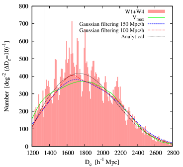
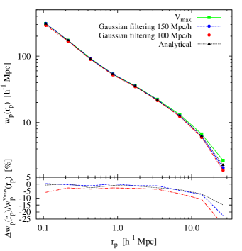
Fig. 6 applies three such approaches to estimate the galaxy radial distribution in the combined W1+W4 sample: the analytical $N(z)$ of Eq. 2; the Gaussian filtering method; and the $V_{\rm max}$ method. This figure shows the recovered $N(D_{c})$ in the random sample with each method, with $D_{c}$ being the radial comoving distance; in practice we work with $N(D_{c})$ instead of $N(z)$. We find that the methods give different estimates of the radial distribution. In the case of the the Gaussian filtering, a kernel size of $150\,h^{-1}\leavevmode\nobreak\ \rm{Mpc}$ is needed to smear out the peaks in the distribution, otherwise the recovered $N(D_{c})$ is still affected by large structures in the field – particularly by that at $D_{c}\simeq 1600\,h^{-1}\leavevmode\nobreak\ \rm{Mpc}$. As expected, the filtering method tends to artificially broaden the $N(D_{c})$ distribution, whereas the analytical and $V_{\rm max}$ methods are much smoother by construction and do not broaden the $N(D_{c})$. We find that the $V_{\rm max}$ estimate shows a slightly flatter distribution at the level of the peak of the distribution, which seems visually to be more consistent with the data. In Fig. 7 we show the effect of using these different estimates of the radial distribution on the shape of the measured correlation function. Gaussian filtering with a kernel size of $150\,h^{-1}\leavevmode\nobreak\ \rm{Mpc}$ and analytical $N(z)$ estimates both yield slightly smaller amplitudes of the projected correlation function on scales of above $10\,h^{-1}\leavevmode\nobreak\ \rm{Mpc}$ than the $V_{\rm max}$ method. Gaussian filtering with a kernel size of $100\,h^{-1}\leavevmode\nobreak\ \rm{Mpc}$ globally underestimates the clustering amplitude on $w_{p}(r_{p})$ as expected, by about $5\%$. The analytical and $V_{\rm max}$ methods give very similar answers, except on scales above $5\,h^{-1}\leavevmode\nobreak\ \rm{Mpc}$ where the former tends to produce a smaller clustering amplitude by $5-15\%$ with respect to the latter. This comparison shows that the $V_{\rm max}$ method is more robust as it uniquely allows us to restore some correlation signal at large separation. For this reason and the fact that it is non-parametric we finally decided to use the $V_{\rm max}$ estimate to measure two-point correlation functions.

Figure 6: Comparison of different estimators of the radial distribution in the combined W1+W4 sample. The filled histogram shows the number of galaxies in fine bins of radial comoving distance. The different curves correspond to random radial distribution realizations normalized to the number of objects in the data, obtained using the $V_{\rm max}$ (solid), Gaussian filtering (dashed and dot-dashed), or analytical (dotted) methods. The vertical line shows the minimum redshift considered in this analysis, i.e. $z=0.5$.

Figure 7: Impact of the use of different estimators of the radial distribution on the shape of the projected correlation function. The projected correlation functions obtained using the $V_{\rm max}$ (solid), Gaussian filtering (dashed and dot-dashed), or analytical (dotted) methods are shown in the top panel, while the relative fractional differences with respect to the $V_{\rm max}$ method are presented in the bottom panel.

5.2.2 Effects related to the angular selection function

The most crucial aspect of the galaxy clustering estimation in VIPERS is to account for the angular selection function. We test our methodology and the different assumptions discussed in Section 4 using the MultiDark mock samples. We measure the accuracy with which we can estimate the two-point correlation function, by confronting the two-point correlation functions measured in the parent catalogues with those measured in the observed mocks when different completeness corrections are included. We measure the average relative difference between the corrected observed mocks and the parent measurement for different statistics. For this test, we consider two galaxy samples encompassing respectively all galaxies in the redshift intervals $0.5<z<0.75$ and $0.75<z<1.0$, using the same redshift distribution in the parent and observed mock samples to construct the radial selection function of the random sample.

Figure 8: Systematic error on the projected correlation function and impact of different corrections. This is calculated considering all VIPERS galaxies in the redshift intervals $0.5<z<0.75$ (top panel) and $0.75<z<1$ (bottom panel).

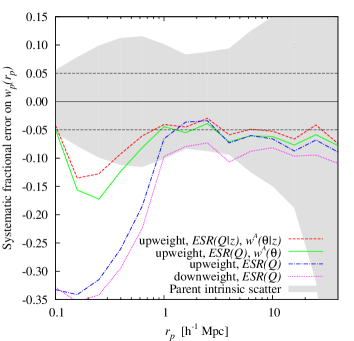
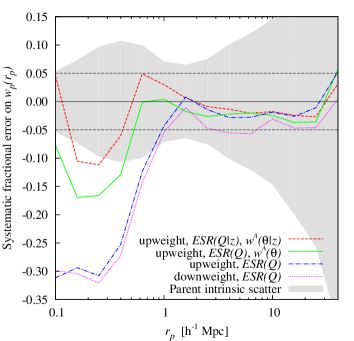
It is common usage in clustering analysis to account for the angular survey completeness by down-weighting the random pair counts. This is usually done by keeping the galaxy counts unweighted and depleting the random sample so as to reproduce the survey angular completeness. The same effect can be achieved by using a uniform angular distribution of random objects but weighting each of them by the inverse of the weight defined in Eq. 6. If we do that and set all the angular pair weights to unity, we obtain the systematic error on $w_{p}(r_{p})$ shown with the dotted curves in Fig. 8. We concentrate first on the results in the interval $0.5<z<0.75$. We can see in this figure that the recovered clustering with this method is underestimated by about $10\%$ at about $1<r_{p}<20\,h^{-1}\leavevmode\nobreak\ \rm{Mpc}$, and then drops rapidly to $35\%$ below. The strong underestimation on small scales is due to the small-scale angular incompleteness effect inside the quadrants. The approach of modulating the random density is dubious in the context of VIPERS, since it treats the sampling variations as a pattern imposed on the large-scale structure. But because of the VIMOS slit allocation, these variations are strongly coupled with the true clustering (i.e. the observed sky distribution of VIPERS galaxies is rather uniform). It is therefore safer if we keep the random sample uniform but upweight the galaxies as described in section 4. In this case, we obtain the dot-dashed lines in Fig. 8: these represent an improved estimation of $w_{p}(r_{p})$, reducing the underestimation by $5-6\%$. As expected, further including the angular pairs weights permits us to remedy in part the underestimation on scales below $1\,h^{-1}\leavevmode\nobreak\ \rm{Mpc}$, where the systematic error reaches $15\%$ (solid lines).

So far, we have used the global survey completeness and angular weights, i.e. neglecting the redshift dependence. As an exercise we use the redshift information from the parent mocks to compute the true redshift-dependent weights and we obtain the dashed lines in the figure. Including the redshift dependence in the weights has the effect of improving the recovery of the projected correlation function by about $2\%$ over all probed scales. However, this improvement is rather modest – indicating that the use of the redshift-independent weights is a good approximation. Our best estimate of $w_{p}(r_{p})$ therefore allows us to recover the true correlation function of the mocks at $0.5<z<0.75$ with about $7\%$ and $16\%$ underestimation respectively above and below $1\,h^{-1}\leavevmode\nobreak\ \rm{Mpc}$. In the redshift interval $0.75<z<1$ (shown in th bottom panel of Fig. 8), we find the same behaviour except that the correlation function is globally better recovered with an underestimation smaller than $2-3\%$ at $r_{p}>0.6\,h^{-1}\leavevmode\nobreak\ \rm{Mpc}$ with the best method.

This test demonstrates that our methodology gives an accurate estimate of the galaxy clustering in VIPERS, even if there remains some residual systematic errors of up to $7\%$ on the scales above 1$\,h^{-1}$ Mpc and $15\%$ on smaller scales. We find that the effect varies with redshift, being more important at the lowest redshifts probed by VIPERS. Overall these systematics remain within the Poisson plus sample variance errors, shown with shaded regions in Fig. 8 and obtained from the standard deviation of $\,w_{p}(r_{p})$ among the parent mock catalogues.

5.3 Impact of possible residual zero-point uncertainties in the photometry

At the time of writing, photometry from the latest CFHTLS release (T0007) has become available (Hudelot et al. 2012). We have compared magnitudes and colours of objects in the VIPERS sample with the new CFHTLS-T0007 photometry. For VIPERS, the most important feature of T0007 compared to previous releases is that each tile in the CFHTLS has now been rescaled to an absolute calibration provided by a new photometric pre-survey taken at CFHT for this purpose. In addition, in order to ensure that seeing variations between tiles and filters are correctly accounted for, this scaling has been done using aperture fluxes that are rescaled based on the seeing on each individual tile; detailed tests at Terapix have shown that mag_auto magnitudes, which are affected by seeing variations, are not sufficiently precise for the percent-level photometric accuracy that is the objective of T0007.

An important consequence of this work for VIPERS is that the effect of seeing variation and photometric calibration errors are now cleanly separated; the stellar-locus fitting technique used to define the VIPERS selection using colours based on mag_auto magnitudes mixes both these effects. To estimate the size of colour and magnitude offsets between T0007 and the actual VIPERS selection (based on T0005) colours of stars on each VIPERS tiles measured from Terapix IQ20 magnitudes (used to calibrate T0007) and from mag_auto magnitudes in both releases have been compared. We find that these offsets shift the colour-colour locus we devised to remove lower-redshift $z<0.5$ galaxies (Guzzo et al. 2013).

We test the effect of these possible variations of the colour selection across the fields in the context of galaxy clustering estimation. For this we use photometric redshifts and quantify the variations in $N(z)$ due to tile-to-tile variations of the colour selection, assuming the T0007 photometry as the reference. When comparing the $N(z_{phot})$ in the different tiles, we find that the redshift distribution varies in shape and amplitude at $z<0.6$ but only in amplitude above. The typical amplitude variations are of the order of about $5\%$ (Guzzo et al. 2013). We then measure the ratio between the $N(z)$ per tile and that averaged over the fields and use it as a redshift-dependent correction factor. To test how these variations of the colour selection affect the measured correlation function, we vary the $N(z)$ in the random sample for each quadrant using the correction factor previously defined on the averaged $N(z)$. The projected correlations obtained with and without this correction are shown in Fig. 9.

Figure 9: Effect of correcting for quadrant-to-quadrant variations of the colour selection in the estimation of the projected correlation function, when using the CFHTLS-T0007 sample as the reference photometric catalogue. The top panel shows the projected correlation functions with and without the correction applied, while the bottom panel presents their relative fractional difference.

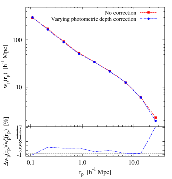
We can see that the correction has the effect of decreasing the amplitude of the projected correlation function by about $2-4\%$ on scales below $10\,h^{-1}\leavevmode\nobreak\ \rm{Mpc}$. We find a similar effect on the redshift-space angle-averaged correlation function $\xi(s)$. The amplitude and direction of the systematic effect follows our expectations, since spurious tile-to-tile fluctuations, if not properly corrected, enhance the amplitude of clustering. This test suggests that indeed such tile-to-tile variations of colour selection are present in the data. It is interesting to note that this systematic effect goes in the opposite direction to the effects of slit-positioning and associated incompleteness. In the end, because this possible effect remains very small, we do not attempt to correct it for the clustering analysis.

6 Real-space clustering

Before studying redshift-space distortions in VIPERS, we begin by looking at the clustering in real space. The projected correlation function for all galaxies in the redshift range $0.5<z<1$ is shown in Fig. 10. It is measured in logarithmic bins of $\Delta\log r_{p}=0.2$ over the scales $0.1<r_{p}<30\,h^{-1}\leavevmode\nobreak\ \rm{Mpc}$. The error bars are estimated from the MultiDark mocks.

Figure 10: Top panel: projected correlation functions of VIPERS galaxies in the redshift interval $0.5<z<1$ for the individual W1 and W4 fields as well as for the combined sample. As a comparison, the $\pm 1\sigma$ dispersion among the mean $\,w_{p}(r_{p})$ in the mocks is shown with the shaded region and the non-linear mass prediction in the assumed cosmology with the dotted curve. Bottom panel: relative difference between the measured $\,w_{p}(r_{p})$ in the W1 and W4 fields and the combined projected correlation function $w^{c}_{p}(r_{p})$.

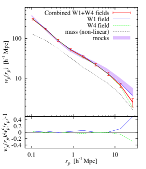
The measured $\,w_{p}(r_{p})$ functions in the W1 and W4 fields are very similar, in particular on scales below 5$\,h^{-1}$ Mpc. The combined projected correlation function in this redshift interval gives an accurate probe of the clustering up to scales of about 30$\,h^{-1}$ Mpc. We can compare the galaxy projected correlation function to predictions for the mass non-linear correlation function and thus estimate the global effective linear bias of these galaxies. We use the HALOFIT (Smith et al. 2003) prescription for the non-linear mass power spectrum to compute the projected correlation function of mass at the mean redshift of the sample. By comparing the amplitudes of the measured galaxy and predicted mass correlations on scales of $r_{p}>1.7\,h^{-1}\leavevmode\nobreak\ \rm{Mpc}$ ($r_{p}>3.4\,h^{-1}\leavevmode\nobreak\ \rm{Mpc}$), and assuming a linear biasing relation of the form $\smash{w_{p}^{\rm gal}=b^{2}_{L}w_{p}^{\rm mass}}$, we obtain a linear bias of $b_{L}=1.35\pm 0.02$ ($b_{L}=1.33\pm 0.02$).

Figure 11: Measured and best-fitting HOD model projected correlation functions $\,w_{p}(r_{p})$, for different luminosity-threshold subsamples of galaxies at $0.7<z<0.9$. The $\,w_{p}(r_{p})$ for the $M_{B}-5\log(h)<-20.5$, $M_{B}-5\log(h)<-21.0$, and $M_{B}-5\log(h)<-21.5$ cases have been multiplied by respectively $2$, $3$, and $4$ to improve the clarity of the figure.

Figure 12: The dependence of $M_{\rm min}$ and $M_{1}$ HOD parameters on redshift and absolute magnitude threshold in $B$-band. The absolute magnitude threshold samples are plot in terms of their implied number density $n_{g}$. The VIPERS results are compared to the pervious measurements performed in the DEEP2 (Zheng et al. 2007), BOSS (White et al. 2011), and CFHTLS (Coupon et al. 2012) surveys.

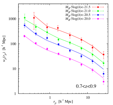
In order to make a detailed interpretation of the observed clustering of galaxies and produce realistic mock samples of the survey, we model our $\,w_{p}(r_{p})$ measurements within the context of the HOD (Seljak 2000; Peacock & Smith 2000; Berlind & Weinberg 2002; Cooray & Sheth 2002). This method defines the mean distribution of galaxies within haloes; under the assumption of the abundance, large-scale bias, and density profile of haloes, one can then completely specify the clustering of galaxies and predict $\,w_{p}(r_{p})$. We define four $B$-band absolute magnitude-threshold samples in the redshift bin $0.7<z<0.9$ in which we measured $\,w_{p}(r_{p})$. We model the projected correlation functions using HOD formalism, within a flat $\Lambda\rm{CDM}$ cosmology with parameters identical to those used in the MultiDark simulation (see Section 5.1). We restrict the fit to scales above $\smash{r_{p}=0.2\,h^{-1}\leavevmode\nobreak\ \rm{Mpc}}$ and below $r_{p}=30\,h^{-1}\leavevmode\nobreak\ \rm{Mpc}$ and correct empirically the measured projected correlation function for the residual underestimation at different scales, using the ratio between the parent and recovered $\,w_{p}(r_{p})$ in the observed mocks for the same galaxy selection. We assume that there is negligible error in taking this small correction to be independent of cosmology. In the fitting procedure we used both the sample number density and $\,w_{p}(r_{p})$ constraints in order to estimate the HOD parameters and their errors by exploring the full parameter space of the model.

In our HOD model the occupation number is parameterized as

$$\left<N_{\rm gal}|m\right>=\left<N_{\rm cen}|m\right>(1+\left<N_{\rm sat}|m\right>)$$ (15)

where $\left<N_{\rm cen}|m\right>$ and $\left<N_{\rm sat}|m\right>$ are the average number of central and satellite galaxies in a halo of mass $m$. This model explicitly assumes that the first galaxy in haloes, when haloes have reached a sufficient mass, has to be central. Central and satellite galaxy occupations are defined as in (Zheng et al. 2005):

$$\left<N_{\rm cen}|m\right> =\frac{1}{2}\left[1+\rm{erf}\left(\frac{\log\leavevmode\nobreak\ m-\log M_{\rm min}}{\sigma_{\log\leavevmode\nobreak\ m}}\right)\right],$$ (16)

$$\left<N_{\rm sat}|m\right> =\left(\frac{m-M_{0}}{M_{1}}\right)^{\alpha}.$$ (17)

where $M_{\rm min}$, $\sigma_{\log\leavevmode\nobreak\ m}$, $M_{0}$, $M_{1}$, and $\alpha$ are the HOD parameters. The parameter $M_{0}$ is generally poorly constrained and we decided in this analysis to fix $M_{0}=M_{\rm min}$ (see also White et al. 2011; de la Torre & Guzzo 2012).

In the halo model formalism, the galaxy power spectrum or two-point correlation function can be written as the sum of two component: the 1-halo term that describes the correlations of galaxies inside haloes and the 2-halo term that characterises the correlations of galaxies sitting in different halos. We follow the formalism of van den Bosch et al. (2013) to define the projected correlation in the context of this model. In particular we use their improved prescriptions for the treatment of the halo-exclusion and residual redshift-space distortions effects on $\,w_{p}(r_{p})$, induced by the finite $\pi_{\rm max}$ values used in the data (van den Bosch et al. 2013). We use the halo bias factor and mass function of Tinker et al. (2008) and Tinker et al. (2010) respectively, and assume that satellite galaxies trace the mass distribution within haloes. We make the assumption of a NFW (Navarro et al. 1996) radial density profile and use the concentration-mass relation obtained by Prada et al. (2012) from the MultiDark simulation. The details of the implementation of the HOD model are given in de la Torre at al. (in preparation).

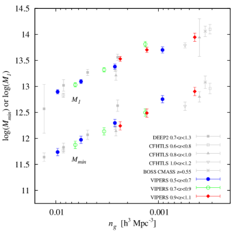
We present in Fig. 11 the measurements and best-fitting HOD models for the four different volume-limited absolute magnitude-threshold samples. We find that the model reproduces the observations well. To have a global characterisation of the clustering properties of galaxies in VIPERS, we extend this modelling to two additional redshift bins at $0.5<z<0.7$ and $0.9<z<1.1$. The best-fitting $M_{\rm min}$ and $M_{1}$ parameters for the different sub-samples are shown in Fig. 12 and compared to previous measurement in the same range of redshift and number density. Because in the different surveys the subsamples are not selected with the same absolute magnitude band of selection, it is convenient to compare the HOD parameters in terms of redshift and the number density probed by each sample. Note that here we compare measurements only from analyses using the same HOD parameterization, although the exact implementation of the models can differ slightly. The VIPERS sample allows us to constraint these parameters with an unprecedented accuracy over the redshift range $0.5<z<1.1$. Our results are consistent with previous measurements, in particular with the DEEP2 (Zheng et al. 2007) and CFHTLS (Coupon et al. 2012) analyses. Our HOD analysis is aimed at modelling the global clustering properties in VIPERS, but we refer the reader to Marulli et al. (2013) and de la Torre et al. (2013, in preparation) for detailed analysis and interpretation of the luminosity and stellar dependence of galaxy clustering and luminosity-dependent halo occupation respectively.

Figure 13: Evolution of the B-band absolute magnitude-dependent HOD. The curves show $\langle N_{\rm gal}(m|z,M_{B})\rangle$ for values of $x=M_{B}-5\log(h)+z$ ranging from $x=-19$ to $x=-22$ with steps of $\Delta x=0.25$, respectively from left to right.

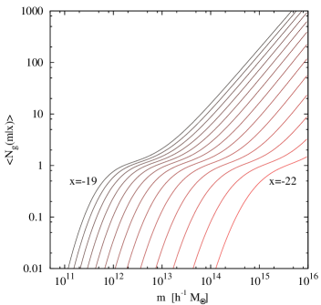
We use the derived HOD parameters to define a global luminosity- and redshift-dependent occupation number which is then used to create accurate HOD mocks of the survey. In order to interpolate between the different redshifts we assume a global luminosity evolution proportional to redshift, so that the magnitude threshold values scale linearly with redshift (Brown et al. 2008; Coupon et al. 2012). We find that one can approximate $\langle N_{\rm gal}(m|z,M_{B})\rangle$ using Eq. 15 with

$$\log M_{\rm min}(x) =10.61\exp(1.49^{-24.66-x})$$ (18)

$$\sigma_{\log m}(x) =0.06\exp(-0.08x+0.34)$$ (19)

$$M_{0}(x) =M_{\rm min}(x)$$ (20)

$$M_{1}(x) =13.5M_{\rm min}(x)$$ (21)

$$\alpha(x) =0.29\exp(-0.05x+0.38)\,,$$ (22)

where $x=M_{B}-5\log(h)+z$. $M_{\rm min}$ and $M_{1}$ are found to be strongly correlated in such a way that $M_{1}$ is approximately equal to $10-20$ times $M_{\rm min}$ depending on the redshift probed and the model implementation (e.g. Beutler et al. 2013). In our analysis we find that $M_{1}(x)$ can be approximated by $13.5$ times $M_{\rm min}(x)$. The function $\langle N_{\rm gal}(m|z,M_{B})\rangle$ is shown in Fig. 13 for the different values of $x$ probed with VIPERS. We checked the consistency of this parameterization and verify that the $\,w_{p}(r_{p})$ predicted by the mocks and the that measured are in good agreement for all probed redshift and luminosity thresholds.

7 Redshift-space distortions

The main goal of VIPERS is to provide with the final sample accurate measurements of the growth rate of structure in two redshift bins between $z=0.5$ and $z=1.2$. The growth rate of structure $f$ can be measured from the anisotropies observed in redshift space in the galaxy correlation function or power spectrum. Although this measurement is degenerate with galaxy bias, the combination $f\sigma_{8}$ is measurable and still allows a fundamental test of modifications of gravity since it is a mixture of the differential and integral growth. In this Section, we present an initial measurement of $f\sigma_{8}$ from the VIPERS first data release.

7.1 Method

With the first epoch VIPERS data we can reliably probe scales below about 35$\,h^{-1}$ Mpc. The use of the smallest non-linear scales, i.e. typically below $10\,h^{-1}\leavevmode\nobreak\ \rm{Mpc}$, is however difficult because of the limitations of current redshift-space distortion models, which cannot describe the non-linear effects that relate the evolution of density and velocity perturbations. However, with the recent developments in perturbation theory and non-linear models for RSD (e.g. Taruya et al. 2010; Reid & White 2011; Seljak & McDonald 2011), we can push our analysis well into mildly non-linear scales and obtain unbiased measurements of $f\sigma_{8}$ while considering minimum scales of $5-10\,h^{-1}\leavevmode\nobreak\ \rm{Mpc}$ (de la Torre & Guzzo 2012).

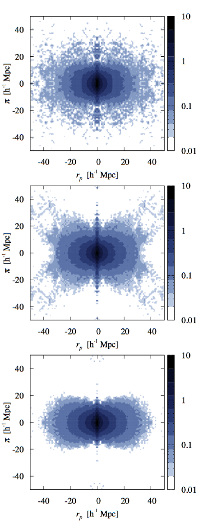
With the VIPERS first data release, we perform an initial redshift-space distortion analysis, considering a single redshift interval of $0.7<z<1.2$ to probe the highest redshifts where the growth rate is little-konwn. We select all galaxies above the magnitude limit of the survey in that interval. The effective pair-weighted mean redshift of the subsample is $z=0.80$. The measured anisotropic correlation function $\,\xi(r_{p},\pi)$ is shown in the top panel of Fig. 14. We have used here a linear binning of $\smash{\Delta r_{p}=\Delta\pi=1\,h^{-1}\leavevmode\nobreak\ \rm{Mpc}}$. One can see in this figure the two main redshift-space distortion effects: the elongation along the line-of-sight, or Finger-of-God effect, which is due to galaxy random motions within virialized objects and the squashing effect on large scales, or Kaiser effect, which represents the coherent large-scale motions of galaxies towards overdensities. The latter effect is the one we are interested in since its amplitude is directly related to the growth rate of perturbations. Compared to the first measurement at such high redshift done with the VVDS survey (Guzzo et al. 2008), this signature is detected with much larger significance, with the flattening being apparent to $r_{p}>30\,h^{-1}\leavevmode\nobreak\ \rm{Mpc}$.

The anisotropic correlation has been extensively used in the literature to measure the growth rate or the distortion parameter $\beta$ (e.g. Hawkins et al. 2003; Guzzo et al. 2008; Cabré & Gaztañaga 2009; Beutler et al. 2012; Contreras et al. 2013). However, with the increasing size and statistical power of redshift surveys, an alternative approach has grown in importance: the use of the multipole moments of the anisotropic correlation function. This approach has the main advantage of reducing the number of observables, compressing the cosmological information contained in the correlation function. In turn, this eases the estimation of the covariance matrices associated with the data. We adopt this methodology in this analysis and fit for the two first non-null moments $\xi_{0}(s)$ and $\xi_{2}(s)$, where most of the relevant information is contained, and ignore the contributions of the more noisy subsequent orders. The multipoles moments are measured from $\xi(s,\mu)$ which is obtained exactly as for $\,\xi(r_{p},\pi)$, except that the redshift-space separation vector $\@vec{s}$ is now decomposed into the polar coordinates $(s,\mu)$ such that $r_{p}=s(1-\mu^{2})^{1/2}$ and $\pi=s\mu$. The multipole moments are related to $\xi(s,\mu)$ as,

$$\xi_{\ell}(s)=\frac{2\ell+1}{2}\int_{-1}^{1}\xi(s,\mu)L_{\ell}(\mu)d\mu,$$ (23)

where $L_{\ell}$ is the Legendre polynomial of order $\ell$. In practice the integration of Eq. 23 is approximated by a Riemann sum over the binned $\xi(s,\mu)$. We use a logarithmic binning in $s$ of $\Delta\log(s)=0.1$ and linear binning in $\mu$ with $\Delta\mu=0.02$.

Figure 14: Anisotropic correlation functions of galaxies at $0.7<z<1.2$. The top panel shows the results for the VIPERS first data release, deduced by the Landy-Szalay estimator counting pairs in cells of side $1\,h^{-1}\leavevmode\nobreak\ \rm{Mpc}$. The lower two panels show the results of two simulations, which span the 68% confidence range on the fitted value of the large-scale flattening (see Section 7.4).

Figure 15: Covariance matrix for the redshift-space distortions analysis. While the lower triangle represents the covariance matrix obtained directly from the MD mocks, the upper triangle corresponds to that obtained after performing shrinkage estimation.

7.2 Covariance matrix, error estimation, and fitting procedure

The different bins in the observed correlation function and associated multipole moments are correlated to some degree, and this must be allowed for in order to fit the measurements with theoretical models. We estimate the covariance matrix of the monopole and quadrupole signal using the MultiDark (MD) and Pinocchio (PN) HOD mocks. The generic elements of the matrix can be evaluated as

$$C_{ij}=\frac{1}{N_{R}-1}\sum_{k=1}^{N_{R}}\left(y^{k}(s_{i})-\bar{y}(s_{i})\right)\left(y^{k}(s_{j})-\bar{y}(s_{j})\right)$$ (24)

where $N_{R}$ is the number of mock realizations, $y(s)$ is the quantity of interest, and the indices $i,j$ run over the data points.

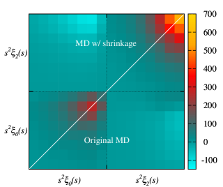
The number of degrees of freedom in the multipole moments varies between $11$ and $15$ depending on the scales considered. Because we have only 26 MD mock realizations, the covariance matrix elements cannot be constrained accurately with the MD mocks only: the covariance matrix is unbiased, but it can have substantial noise. In order to mitigate the noise and obtain an accurate estimate of the covariance matrix, we apply the shrinkage method (Pope & Szapudi 2008), using the covariance matrix obtained with the 200 PN mocks as the target matrix. The PN mocks are more numerous and therefore each element of the associated covariance matrix is very well constrained, although the covariance may be biased to some extent. This bias is related to inaccuracies in the predicted moments, which are mainly driven by the limited accuracy of the Zel’dovich approximation used in the PN mocks to predict the peculiar velocity field. The shrinkage technique allows the optimal combination of an empirical estimate of the covariance with a target covariance, minimising the total mean squared error compared to the true underlying covariance. An optimal covariance matrix $C$ is then obtained with

$$C=\lambda T+(1-\lambda)S,$$ (25)

where $\lambda$ is the shrinkage intensity and the target ${T}$ and empirical ${S}$ covariance matrices correspond respectively to those obtained from the PN and MD mocks. $\lambda$ is calculated from (Pope & Szapudi 2008)

$$\lambda=\frac{\sum_{i,j}{\rm Cov}(S_{ij},S_{ij})-{\rm Cov}(T_{ij},S_{ij})}{\sum_{i,j}({T}_{ij}-{S}_{ij})^{2}},$$ (26)

where ${\rm Cov}(A_{ij},B_{ij})$ stands for the covariance between the elements $(i,j)$ of the matrices $A$ and $B$. We note that, since the empirical and target matrices are independent, the term ${\rm Cov}(T_{ij},S_{ij})$ vanishes in the numerator of Eq. 26. The effect of shrinkage estimation on the MD covariance matrix is shown in Fig. 15.

To measure the growth rate of structure we perform a maximum likelihood analysis of the data given models of redshift-space distortions by adopting the likelihood function $\mathcal{L}$:

$$-2\ln{\mathcal{L}}=\sum_{i=1}^{N_{p}}\sum_{j=1}^{N_{p}}\Delta_{i}C^{-1}_{ij}\Delta_{j},$$ (27)

where $N_{p}$ is the number of points in the fit, $\Delta$ is the data-model difference vector, and $C$ is the covariance matrix. The likelihood is performed on the quantity $y(s)=s^{2}\xi_{\ell}(s)$, rather than simply $y(s)=\xi_{\ell}(s)$ to reduce the range of variations of multipole values at different $s$ in the fit. In the end, the quantity which is matched with model predictions is the concatenation of $s^{2}\xi_{0}$ and $s^{2}\xi_{2}$ for the set of separations considered.

As a final remark, we note that we use the direct inverse of the covariance matrix without applying the correction discussed by Hartlap et al. (2007), as it is not clear how the size of the correction is affected by the shrinkage estimation technique. The resulting errors derived from the likelihood are well matched to the distribution of best-fit values from the mocks, which gives us confidence that only a small correction, if any, would be necessary.

Figure 16: Systematic and statistical errors on $f\sigma_{8}$ obtained from the mock samples, for different models and minimum scales $s_{min}$ in the fit. The horizontal dashed line shows the expectation value while the shaded area marks the $15\%$ region around the fiducial value. Note that the points have been slightly displaced horizontally around $s_{min}$ values of $5\,h^{-1}\leavevmode\nobreak\ \rm{Mpc}$, $6\,h^{-1}\leavevmode\nobreak\ \rm{Mpc}$, and $7\,h^{-1}\leavevmode\nobreak\ \rm{Mpc}$ to improve the clarity of the figure.

7.3 Models

The formalism that describes redshift-space anisotropies in the power spectrum can be derived from writing the mass density conservation in real and redshift space (Kaiser 1987). In particular, in the plane-parallel approximation, which is assumed in this analysis, the anisotropic power spectrum of mass has the general compact form (Scoccimarro et al. 1999)

$$P^{s}(k,\nu) ={}\int\frac{d^{3}\@vec{r}}{(2\pi)^{3}}e^{-i\@vec{k}\cdot\@vec{r}}\left<e^{-ikf\nu\Delta u_{\parallel}}\times\right.$$

$$\left.[\delta(\@vec{x})+\nu^{2}f\theta(\@vec{x})][\delta(\@vec{x}^{\prime})+\nu^{2}f\theta(\@vec{x}^{\prime})]\right>$$ (28)

where $\nu=k_{\parallel}/k$, $u_{\parallel}(\@vec{r})=-v_{\parallel}(\@vec{r})/(faH(a))$, $v_{\parallel}(\@vec{r})$ is the line-of-sight component of the peculiar velocity, $\delta$ is the density field, $\theta$ is the divergence of the velocity field, $\Delta u_{\parallel}=u_{\parallel}(\@vec{x})-u_{\parallel}(\@vec{x}^{\prime})$ and $\@vec{r}=\@vec{x}-\@vec{x}^{\prime}$. Although exact, Eq. 28 is impractical for direct use on redshift survey measurements and several models have been proposed to approximate it. In the assumption that galaxies linearly trace the underlying mass density field with a bias $b$, we can build three empirical models. These take the form,

$$P_{g}^{s}(k,\nu)=D(k\nu\sigma_{v})P_{K}(k,\nu;f,b)$$ (29)

where,

$$D(k\nu\sigma_{v})=\left\{\begin{array}[]{lcl}\exp(-(k\nu\sigma_{v})^{2})\\ \\ 1/(1+(k\nu\sigma_{v})^{2})\end{array}\right.$$ (33)

and,

$$P_{K}(k,\nu;f,b)=\hskip 199.16928pt$$

$$\left\{\begin{array}[]{lcl}\hbox to0.0pt{$b^{2}P_{\rm{\delta\delta}}(k)+2\nu^{2}fbP_{\rm{\delta\delta}}(k)+\nu^{4}f^{2}P_{\rm{\delta\delta}}(k)$\hss}\hskip 156.49014pt{\rm(model\leavevmode\nobreak\ A)}\\ \\ \hbox to0.0pt{$b^{2}P_{\rm{\delta\delta}}(k)+2\nu^{2}fbP_{\rm{\delta\theta}}(k)+\nu^{4}f^{2}P_{\rm{\theta\theta}}(k)$\hss}\hskip 156.49014pt{\rm(model\leavevmode\nobreak\ B)}\\ \\ b^{2}P_{\rm{\delta\delta}}(k)+2\nu^{2}fbP_{\rm{\delta\theta}}(k)+\nu^{4}f^{2}P_{\rm{\theta\theta}}(k)\\ \hbox to0.0pt{$+C_{A}(k,\nu;f,b)+C_{B}(k,\nu;f,b).$\hss}\hskip 156.49014pt{\rm(model\leavevmode\nobreak\ C)}\end{array}\right.$$ (40)

In these equations $P_{\rm{\delta\delta}}$, $P_{\rm{\delta\theta}}$, $P_{\rm{\theta\theta}}$ are respectively the non-linear mass density-density, density-velocity divergence, and velocity divergence-velocity divergence power spectra and $\sigma_{v}$ is an effective pairwise velocity dispersion that we can fit for and then treat as a nuisance parameter. The expressions for $C_{A}(k,\nu;f,b)$ and $C_{B}(k,\nu;f,b)$ are given in appendix A of de la Torre & Guzzo (2012). These empirical models can be seen in configuration space, as a convolution of a damping function $D(k\mu\sigma_{v})$, which we assume to be Gaussian or Lorentzian in Fourier space, and a term involving the density and velocity divergence correlation functions and their spherical Bessel transforms. While the first term essentially (but not only) describes the Finger-of-God effect, the second, $P_{K}(k,\nu,b)$, describes the Kaiser effect. We note that model A is the classical dispersion model (Peacock & Dodds 1994) based on the linear Kaiser (1987) model; model B is the generalisation proposed by Scoccimarro (2004) that accounts for the non-linear coupling between the density and velocity fields, making explicitly appearing the velocity divergence auto-power spectrum and density–velocity divergence cross-power spectrum; model C is an extension of model B that contains the two additional correction terms proposed by Taruya et al. (2010) to correctly account for the coupling between the Kaiser and damping terms. We refer the reader to de la Torre & Guzzo (2012) for a thorough description of these models.

In the end, the model $\xi^{s}_{\ell}(s)$ are obtained from their Fourier counterparts,

$$P^{s}_{\ell}(k)=\frac{2\ell+1}{2}\int_{-1}^{1}d\nu P_{g}^{s}(k,\nu)L_{\ell}(\nu),$$ (41)

as

$$\xi^{s}_{\ell}(s)=i^{\ell}\int\frac{dk}{2\pi^{2}}k^{2}P^{s}_{\ell}(k)j_{\ell}(ks),$$ (42)

where $j_{\ell}$ denotes the spherical Bessel functions.

The redshift-space distortion models involve the knowledge of the underlying mass non-linear power spectra of density and velocity divergence at the effective redshift of the sample. Although the real-space non-linear correlation function of galaxies can be recovered from the deprojection of the observed projected correlation function (e.g. Bianchi et al. 2012) and thus be used to some extent as an input of the model (e.g. Hamilton 1992), it is not feasible for the more advanced models which involve the velocity divergence power spectrum. The non-linear power spectra can however be predicted from perturbation theory or simulations for different cosmological models. In the case of a $\Lambda\rm{CDM}$ cosmology, the shape of the non-linear power spectra depends on the parameters $P=(\Omega_{m},\Omega_{b},h,n_{s},\sigma_{8})$ and can be obtained to a great accuracy from semi-analytical prescriptions such as HALOFIT. In this analysis we use the latest calibration of HALOFIT by Bird et al. (2012) to obtain $P_{\rm{\delta\delta}}$ and use the fitting functions of Jennings (2012) to predict $P_{\rm{\theta\theta}}$ and $P_{\rm{\delta\theta}}$ from $P_{\rm{\delta\delta}}$. The latter fitting functions are accurate at the few percent level up to $k\simeq 0.3$ at $z=1$.

In the models, the bias and growth rate parameters $b$ and $f$ are degenerate with the normalization of the power spectrum parameter $\sigma_{8}$. Thus, in practice only the combination of $b\sigma_{8}$ and $f\sigma_{8}$ can be constrained if no assumption is made on the actual value of $\sigma_{8}$. This can be done by renormalizing the power spectra in the models so that $P_{xx}(k,z)\rightarrow P_{xx}(k,z)/\sigma_{8}^{2}(z)$, thus reparameterizing the models such that the parameters $(b,f)$ are replaced by $(b\sigma_{8},f\sigma_{8})$ in Eq. 29. This parameterization can be used for model A and B, although not for model C in which the correction term $C_{A}$ involves the additional combinations: $b^{2}f\sigma_{8}^{4}$, $bf^{2}\sigma_{8}^{4}$, and $f^{3}\sigma_{8}^{4}$ (see Taruya et al. 2010; de la Torre & Guzzo 2012). The correction term $C_{A}$, which partially describes the effects of the non-linear coupling between the damping and Kaiser terms, mostly affects the monopole and quadrupole moments of the redshift-space power spectrum on scales of $k>0.1$ (Taruya et al. 2010). Therefore, in principle $C_{A}$ could help breaking the degeneracy between $f$ and $\sigma_{8}$ although this has to be verified in detail. In the end, in the case of model C we decided to treat $(f,b,\sigma_{8},\sigma_{v})$ as separate parameters in the fit.

7.4 Detailed tests against mock data

Figure 17: Monopole and quadrupole moments of the redshift-space correlations, as a function of scale. The shallow curves show the results for the 26 individual MultiDark simulation mocks; the points are for the measured VIPERS data at $0.7<z<1.2$, with assigned error bars based on the scatter in the mocks. The solid and dotted lines correspond to the best fitting models to the data for model B with Gaussian or Lorentzian damping function respectively.

Figure 18: Marginalized likelihood distribution of $f\sigma_{8}$ in the data (solid curve) and distribution of fitted values of $f\sigma_{8}$ for the 26 individual MultiDark simulation mocks (histogram). These curves show a preferred value and a dispersion in the data that is consistent at the $1\sigma$ level with the distribution over the mocks.

Figure 19: A plot of $f\sigma_{8}$ versus redshift, showing VIPERS result contrasted with a compilation of recent measurements. The previous results from 2dFGRS (Hawkins et al. 2003), 2SLAQ (Ross et al. 2007), VVDS (Guzzo et al. 2008), SDSS LRG (Cabré & Gaztañaga 2009; Samushia et al. 2012), WiggleZ (Blake et al. 2012), BOSS (Reid et al. 2012), and 6dFGS (Beutler et al. 2012) surveys are shown with the different symbols (see inset). The thick solid (dashed) curve corresponds to the prediction for General Relativity in a $\Lambda\rm{CDM}$ model with WMAP9 (Planck) parameters, while the dotted, dot-dashed, and dot-dot-dashed curves are respectively Dvali-Gabadaze-Porrati (Dvali et al. 2000), coupled dark energy, and $f(R)$ model expectations. For these models, the analytical growth rate predictions given in di Porto et al. (2012) have been used.

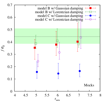
We perform the redshift-space distortion analysis of the VIPERS data in the context of a flat $\Lambda\rm{CDM}$ cosmological model. Before considering the redshift-space distortions in the data, we first test the methodology and expected errors on $f\sigma_{8}$ using the mock samples. We fix the shape of the mass non-linear power spectrum to that of the simulation (since the observed real-space correlations are of high accuracy) and perform a likelihood analysis of each individual MD mock. In the case of model C we also fix the normalisation of the power spectrum as discussed above. The distribution of best-fitting $f\sigma_{8}$ values gives us a direct estimate of the probability distribution function of the parameter for a given fitting method, and serves as a check on the errors from the full likelihood function. We estimate the median and $68\%$ confidence region of the distribution. These are shown in Fig. 16 for the different models presented in the previous section and for various minimum scales $s_{min}$ in the fit.

Model A is known to be the most biased model (e.g. Okumura & Jing 2011; Bianchi et al. 2012; de la Torre & Guzzo 2012) and our results confirm these findings. We thus decided not to describe in the following the detailed behaviour of this model and focus on models B and C. We find that in general model B tends to be less biased than model C, which is surprising at first sight as model C is the most advanced and supposed to be the most accurate (Kwan et al. 2012; de la Torre & Guzzo 2012). This could be due to the quite restricted scales that we consider and the limited validity of its implementation on scales below $s\simeq 10\,h^{-1}\leavevmode\nobreak\ \rm{Mpc}$, as the maximum wavenumber to which we can predict $P_{\rm{\delta\theta}}$ and $P_{\rm{\theta\theta}}$ is about $k=0.3$. We defer the investigation of this issue to the redshift-space distortion analysis of the final sample and concentrate here on model B. The shape of the damping function in the models also affects the recovered $f\sigma_{8}$, as expected given the minimum scales we consider, although in the case of model B the change in $f\sigma_{8}$ is at most $5\%$. Including smaller scales in the fit reduces the statistical error but at the price of slightly larger systematic error. Therefore from this test we decided to use model B and a compromise value for the minimum scale of $s_{min}=6\,h^{-1}\leavevmode\nobreak\ \rm{Mpc}$.

7.5 The VIPERS result for the growth rate

These comprehensive tests of our methodology give us confidence that we can now proceed to the analysis of the real VIPERS data and expect to achieve results for the growth rate that are robust, and which can be used as a trustworthy test of the nature of gravity at high redshifts.

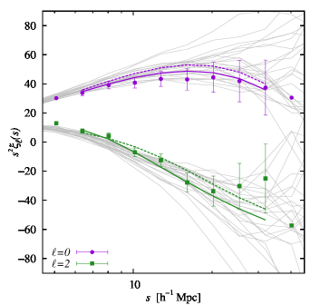
As explained earlier, we assume a fixed shape of the mass power spectrum consistent with the cosmological parameters obtained from WMAP9 (Hinshaw et al. 2012) and perform a maximum likelihood analysis on the data, considering variations in the parameters that are not well determined externally. The best-fitting models are shown in Fig. 17 when considering either a Gaussian or a Lorentzian damping function. Although the mock samples tend to slightly prefer models with Lorentzian damping as seen in Fig. 16, we find that the Gaussian damping provides a much better fit to the real data and we decided to quote the corresponding $f\sigma_{8}$ as our final measurement.

We measure a value of

$$f(z=0.8)\sigma_{8}(z=0.8)=0.47\pm 0.08,$$ (43)

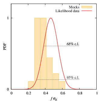
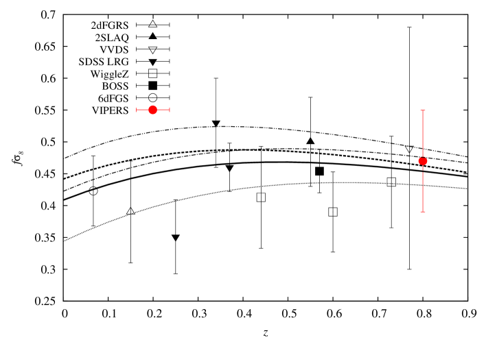
which is consistent with the General Relativity prediction in a flat $\Lambda\rm{CDM}$ Universe with cosmological parameters given by WMAP9, for which the expected value is $f(0.8)\sigma_{8}(0.8)=0.45$. We find that our result is not significantly altered if we adopt a Planck cosmology (Planck Collaboration et al. 2013) for the shape of the mass power spectrum, changing our best-fitting $f\sigma_{8}$ by only $0.2\%$. This shows that given the volume probed by the survey, we are relatively insensitive to the additional Alcock-Paczynski distortions (Alcock & Paczynski 1979) on the correlation function. The marginalised likelihood distribution of $f\sigma_{8}$ is shown superimposed on the mock results in Fig. 18. We see that the preferred values of the growth rate are consistent with the mocks, in terms of the width of the likelihood function being comparable to the scatter in mock fitted values. To illustrate the degree of flattening of the anisotropic correlation function induced by structure growth, we show in the middle and bottom panels of Fig. 14 $\,\xi(r_{p},\pi)$ for two MD mocks for which the measured $f\sigma_{8}$ roughly coincide with the $1\sigma$ limits around the best-fit $f\sigma_{8}$ value obtained in the data. We therefore conclude that the initial VIPERS data prefer a growth rate that is fully consistent with predictions based on standard gravity. Our measurement of $f\sigma_{8}$ is also in good agreement with previous measurements at lower redshifts from 2dFGRS (Hawkins et al. 2003), 2SLAQ (Ross et al. 2007), VVDS (Guzzo et al. 2008), SDSS LRG (Cabré & Gaztañaga 2009; Samushia et al. 2012), WiggleZ (Blake et al. 2012), BOSS (Reid et al. 2012), and 6dFGS (Beutler et al. 2012) surveys as shown in Fig. 19. In particular, it is compatible within $1\sigma$ with the results obtained in the VVDS (Guzzo et al. 2008) and WiggleZ (Blake et al. 2012) surveys at a similar redshift, although WiggleZ measurements tend to suggest lower $f\sigma_{8}$ values, smaller than expected in standard gravity (but see Contreras et al. 2013).

Finally we compare our measurement to the predictions of three of the most plausible modified gravity models studied in di Porto et al. (2012). We consider Dvali-Gabadaze-Porrati (DGP, Dvali et al. 2000), $f(R)$, and coupled dark energy models and show their predictions in Fig. 19 (see di Porto et al. 2012, for the detail of their analytic predictions). We find that our $f\sigma_{8}$ measurement is currently unable to discriminate between these modified gravity models and standard gravity given the size of the uncertainty, although we expect to improve the constraints with the analysis of the VIPERS final dataset.

8 Conclusions

We have analysed in this paper the global real- and redshift-space clustering properties of galaxies in the VIPERS survey first data release. We have presented the selection function of the survey and the corrections that are needed in order to derive estimates of galaxy clustering that are free of observational biases. This has been achieved by using a large set of simulated mock realizations of the survey to quantify in detail the systematics and uncertainties on our clustering measurements.

The first data release of about $54000$ galaxies at $0.5<z<1.2$ in the VIPERS survey allows a measurement of the real-space clustering of galaxies through the measurement of the projected two-point correlation function, to an unprecedented accuracy over $0.5<z<1.2$. This permits detailed modelling of the halo occupation distribution at these redshifts to be carried out. From an initial HOD modelling of $B$-band luminosity selected samples, we have been able to accurately determine the characteristic halo masses for halo occupation in the redshift interval $0.5<z<1.0$. These measurements are invaluable for creating realistic synthetic mock samples.

The main goal of VIPERS is to provide an accurate measurement of the growth rate of structure through the characterisation of the redshift-space distortions in the galaxy clustering pattern. With the first data release we have been able to provide an initial measurement of $f\sigma_{8}$ at $z=0.8$. We find a value of $f\sigma_{8}=0.47\pm 0.08$ which is in agreement with previous measurements at lower redshifts. This allows us to put a new constraint on gravity at the epoch when the Universe was almost half its present age. Our measurement of $f\sigma_{8}$ is statistically consistent with a Universe where the gravitational interactions between structures on $10\,h^{-1}\leavevmode\nobreak\ \rm{Mpc}$ scales can be described by Einstein’s theory of gravity.

The present dataset represents the half-way stage of the VIPERS project, and the final survey will be large enough to subdivide our measurements and follow the evolution of $f\sigma_{8}$ out to redshift one. This will allow us to address some issues such as the suggestion from the WiggleZ measurements that $f\sigma_{8}$ is lower than expected at $z>0.5$. Our measurement at $z=0.8$ already argues against such a trend to some extent, but the larger redshift baseline and tighter errors from the final VIPERS dataset can be expected to deliver a definitive verdict on the the high-redshift evolution of the strength of gravity.

Appendix A Galaxy mock catalogue construction

We provide in this appendix some details about the method that we used to create realistic galaxy catalogues based on the Halo Occupation Distribution (HOD) and Stellar-to-Halo Mass Relation (SHMR) formalisms. From the MultiDark simulation and Pinocchio halo lightcones described in Section 5.1, we created two types of galaxy mock catalogues: one containing $B$-band absolute magnitudes and associated quantities, and a second one containing stellar masses. We note that the stellar mass mock catalogues have not been explicitly used in this analysis, but in the accompanying VIPERS analyses of Marulli et al. (2013) and Davidzon et al. (2013).

For the first set of catalogues we use the HOD formalism and populated dark matter haloes according to their mass by specifying the absolute $B$-band magnitude-dependent halo occupation. We parametrised the latter using Eq. 15 and used the HOD parameters obtained from the data and given in Section 6. We positioned central galaxies at halo centres with probability given by a Bernoulli distribution function with mean taken from Eq. 16 and assigned host halo mean velocities to these galaxies. The number of satellite galaxies per halo is set to follow a Poisson distribution with mean given by Eq. 17. We assumed that satellite galaxies follow the spatial and velocity distribution of mass and randomly distributed their halo-centric radial position so as to reproduce a Navarro et al. (1996) (NFW) radial profile,

$$\rho_{NFW}(r|m)\propto\left(\frac{c_{dm}(m)r}{r_{v}(m)}\right)^{-1}\left(1+\frac{c_{dm}(m)r}{r_{v}(m)}\right)^{-2},$$ (44)

where $c_{dm}$ is the concentration parameter and $r_{v}(m)$ is the virial radius defined as

$$r_{v}(m)=\left(\frac{3m}{4\pi\bar{\rho}(z)\Delta_{NL}}\right)^{1/3}.$$ (45)

In this equation, $\bar{\rho}(z)$ is the mean matter density at redshift $z$ and $\Delta_{NL}=200$ is the critical overdensity for virialisation in our definition. We assumed the mass-concentration relation of Bullock et al. (2001):

$$c_{dm}(m,z)=\frac{c_{0}}{1+z}\left(\frac{m}{m_{*}}\right)^{-0.13},$$ (46)

where $c_{0}=11$ and $m_{*}$ is the non-linear mass scale at $z=0$ defined such as $\sigma(m_{*},0)=\delta_{c}$. Here $\delta_{c}$ and $\sigma(m,0)$ are respectively the critical overdensity (we fixed $\delta_{c}=1.686$) and the standard deviation of mass fluctuations at $z=0$. The latter is defined as

$$\sigma^{2}(m,z)=\int_{0}^{\infty}\frac{dk}{k}\frac{k^{3}P(k,z)}{2\pi^{2}}|W(kR)|^{2}\,\,\,\,,$$ (47)

where $R=\left[3m/\left(4\pi\bar{\rho}(z)\right)\right]^{1/3}$, $P(k,z)$ is the linear mass power spectrum at redshift $z$ in the adopted cosmology, and $W(x)$ is the Fourier transform of a top-hat filter. In order to assign satellite galaxy velocities, we assumed halo isotropy and sphericity, and drew velocities from Gaussian distribution functions along each Cartesian dimension with velocity dispersion given by (van den Bosch et al. 2004):

$$\sigma^{2}_{sat}(r|m) ={}\frac{1}{\rho_{NFW}(r|m)}\int_{r}^{\infty}\rho_{NFW}(r|m)\frac{d\psi}{dr}dr$$ (48)

$$={}\frac{Gm}{r_{v}}\frac{c_{dm}}{f(c_{dm})}\left(\frac{c_{dm}r}{r_{v}}\right)\left(1+\frac{c_{dm}r}{r_{v}}\right)^{2}I(r/rs),$$ (49)

where $\psi(r)$ is the gravitational potential, $G$ is the gravitational constant, $f(x)=\ln(1+x)-x/(1+x)$, and

$$I(x)=\int_{x}^{\infty}\frac{f(t)dt}{t^{3}(1+t)^{2}}.$$ (50)

In these mocks, the absolute $B$-band magnitude for each galaxy was obtained following Skibba et al. (2006). From the mean rest-frame $B-i^{\prime}$ colour and K-corrections observed in the data we then derived absolute and apparent $i^{\prime}$-band magnitudes for each simulated galaxy.

For the mock catalogues with stellar masses, we followed the SHMR approach which is based on the assumption of a monotonic relation between halo/subhalo masses and the stellar masses of the galaxies associated with them. We first populated the haloes in the lightcones with subhaloes. For this we randomly distributed subhaloes around each distinct halo following a NFW profile so that their number density satisfies the subhalo mass function of Giocoli et al. (2010):

$$\frac{dN(m_{\rm{sub}}|m)}{d\ln m_{\rm{sub}}}=N_{0}\xi^{\alpha}\exp(-\beta\xi^{3}),$$ (51)

where $m_{\rm{sub}}$ is the subhalo mass, $\xi=m_{\rm{sub}}/m$, $\alpha=-0.8$, $\beta=12.2715$, and $N_{0}=0.18$. We then assigned a galaxy to each halo and subhalo, with a stellar mass given by the SHMR of Moster et al. (2013). The galaxy velocities were assigned in a similar way as for the HOD catalogues, with galaxies associated with distinct haloes and subhaloes being considered as central and satellite galaxies respectively.

References

- Alcock & Paczynski (1979) Alcock, C. & Paczynski, B. 1979, Nature, 281, 358
- Berlind & Weinberg (2002) Berlind, A. A. & Weinberg, D. H. 2002, ApJ, 575, 587
- Beutler et al. (2013) Beutler, F., Blake, C., Colless, M., et al. 2013, MNRAS, 429, 3604
- Beutler et al. (2012) Beutler, F., Blake, C., Colless, M., et al. 2012, MNRAS, 423, 3430
- Bianchi et al. (2012) Bianchi, D., Guzzo, L., Branchini, E., et al. 2012, MNRAS, 427, 2420
- Bird et al. (2012) Bird, S., Viel, M., & Haehnelt, M. G. 2012, MNRAS, 420, 2551
- Blake et al. (2012) Blake, C., Brough, S., Colless, M., et al. 2012, MNRAS, 425, 405
- Bottini et al. (2005) Bottini, D., Garilli, B., Maccagni, D., et al. 2005, PASP, 117, 996
- Brown et al. (2008) Brown, M. J. I., Zheng, Z., White, M., et al. 2008, ApJ, 682, 937
- Bullock et al. (2001) Bullock, J. S., Kolatt, T. S., Sigad, Y., et al. 2001, MNRAS, 321, 559
- Cabré & Gaztañaga (2009) Cabré, A. & Gaztañaga, E. 2009, MNRAS, 393, 1183
- Carlson & White (2010) Carlson, J. & White, M. 2010, ApJS, 190, 311
- Cole (2011) Cole, S. 2011, MNRAS, 416, 739
- Colless et al. (2001) Colless, M., Dalton, G., Maddox, S., et al. 2001, MNRAS, 328, 1039
- Colless et al. (2003) Colless, M., Peterson, B. A., Jackson, C., et al. 2003, ArXiv Astrophysics e-prints
- Contreras et al. (2013) Contreras, C., Blake, C., Poole, G. B., et al. 2013, MNRAS, 683
- Cooray & Sheth (2002) Cooray, A. & Sheth, R. 2002, Phys. Rep, 372, 1
- Coupon et al. (2012) Coupon, J., Kilbinger, M., McCracken, H. J., et al. 2012, A&A, 542, A5
- Davidzon et al. (2013) Davidzon, I., Bolzonella, M., Coupon, J., et al. 2013, A&A submitted, ArXiv e-print 1303.3808
- Davis & Huchra (1982) Davis, M. & Huchra, J. 1982, ApJ, 254, 437
- de la Torre & Guzzo (2012) de la Torre, S. & Guzzo, L. 2012, MNRAS, 427, 327
- de la Torre et al. (2011) de la Torre, S., Meneux, B., De Lucia, G., et al. 2011, A&A, 525, A125
- de la Torre & Peacock (2012) de la Torre, S. & Peacock, J. A. 2012, MNRAS submitted, ArXiv e-print 1212.3615
- di Porto et al. (2012) di Porto, C., Amendola, L., & Branchini, E. 2012, MNRAS, 419, 985
- Dvali et al. (2000) Dvali, G., Gabadadze, G., & Porrati, M. 2000, Physics Letters B, 485, 208
- Fisher et al. (1994) Fisher, K. B., Davis, M., Strauss, M. A., Yahil, A., & Huchra, J. P. 1994, MNRAS, 267, 927
- Garilli et al. (2008) Garilli, B., Le Fèvre, O., Guzzo, L., et al. 2008, A&A, 486, 683
- Garilli et al. (2012) Garilli, B., Paioro, L., Scodeggio, M., et al. 2012, PASP, 124, 1232
- Giocoli et al. (2010) Giocoli, C., Tormen, G., Sheth, R. K., & van den Bosch, F. C. 2010, MNRAS, 404, 502
- Goranova et al. (2009) Goranova, Y., Hudelot, P., Magnard, F., et al. 2009, The CFHTLS T0006 Release, http://terapix.iap.fr/cplt/table_syn_T0006.html
- Guo et al. (2012) Guo, H., Zehavi, I., & Zheng, Z. 2012, ApJ, 756, 127
- Guzzo et al. (2008) Guzzo, L., Pierleoni, M., Meneux, B., et al. 2008, Nature, 451, 541
- Guzzo et al. (2013) Guzzo, L., Scodeggio, M., Garilli, B., et al. 2013, A&A submitted, ArXiv e-print 1303.2623
- Hamilton (1992) Hamilton, A. J. S. 1992, ApJ, 385, L5
- Hamilton (1993) Hamilton, A. J. S. 1993, ApJ, 417, 19
- Hartlap et al. (2007) Hartlap, J., Simon, P., & Schneider, P. 2007, A&A, 464, 399
- Hawkins et al. (2003) Hawkins, E., Maddox, S., Cole, S., et al. 2003, MNRAS, 346, 78
- Hinshaw et al. (2012) Hinshaw, G., Larson, D., Komatsu, E., et al. 2012, ArXiv e-prints
- Hudelot et al. (2012) Hudelot, P., Goranova, Y., Mellier, Y., et al. 2012, T0007: The Final CFHTLS Release, http://terapix.iap.fr/cplt/T0007/doc/T0007-doc.pdf
- Iovino et al. (2010) Iovino, A., Cucciati, O., Scodeggio, M., et al. 2010, A&A, 509, A40+
- Jain & Khoury (2010) Jain, B. & Khoury, J. 2010, Annals of Physics, 325, 1479
- Jennings (2012) Jennings, E. 2012, MNRAS, 427, L25
- Kaiser (1987) Kaiser, N. 1987, MNRAS, 227, 1
- Kovač et al. (2010) Kovač, K., Lilly, S. J., Cucciati, O., et al. 2010, ApJ, 708, 505
- Kwan et al. (2012) Kwan, J., Lewis, G. F., & Linder, E. V. 2012, ApJ, 748, 78
- Landy & Szalay (1993) Landy, S. D. & Szalay, A. S. 1993, ApJ, 412, 64
- Le Fèvre et al. (2003) Le Fèvre, O., Saisse, M., Mancini, D., et al. 2003, in Proc. SPIE, ed. M. Iye & A. F. M. Moorwood, Vol. 4841, 1670–1681
- Linder & Cahn (2007) Linder, E. V. & Cahn, R. N. 2007, Astroparticle Physics, 28, 481
- Malek et al. (2013) Malek, K., Solarz, A., Pollo, A., et al. 2013, A&A in press, ArXiv e-print 1303.2621
- Marchetti et al. (2013) Marchetti, A., Granett, B. R., Guzzo, L., et al. 2013, MNRAS, 428, 1424
- Marulli et al. (2013) Marulli, F., Bolzonella, M., Branchini, E., et al. 2013, A&A in press, ArXiv e-print 1303.2633
- McDonald & Seljak (2009) McDonald, P. & Seljak, U. 2009, J. Cosmology Astropart. Phys., 10, 7
- Meneux et al. (2006) Meneux, B., Le Fèvre, O., Guzzo, L., et al. 2006, A&A, 452, 387
- Monaco et al. (2013) Monaco, P., Sefusatti, E., Borgani, S., et al. 2013, MNRAS
- Monaco et al. (2002) Monaco, P., Theuns, T., & Taffoni, G. 2002, MNRAS, 331, 587
- Moster et al. (2013) Moster, B. P., Naab, T., & White, S. D. M. 2013, MNRAS, 428, 3121
- Navarro et al. (1996) Navarro, J. F., Frenk, C. S., & White, S. D. M. 1996, ApJ, 462, 563
- Okumura & Jing (2011) Okumura, T. & Jing, Y. P. 2011, ApJ, 726, 5
- Peacock & Dodds (1994) Peacock, J. A. & Dodds, S. J. 1994, MNRAS, 267, 1020
- Peacock & Smith (2000) Peacock, J. A. & Smith, R. E. 2000, MNRAS, 318, 1144
- Planck Collaboration et al. (2013) Planck Collaboration, Ade, P. A. R., Aghanim, N., et al. 2013, ArXiv e-prints
- Pope & Szapudi (2008) Pope, A. C. & Szapudi, I. 2008, MNRAS, 389, 766
- Prada et al. (2012) Prada, F., Klypin, A. A., Cuesta, A. J., Betancort-Rijo, J. E., & Primack, J. 2012, MNRAS, 423, 3018
- Reid et al. (2012) Reid, B. A., Samushia, L., White, M., et al. 2012, MNRAS, 426, 2719
- Reid & White (2011) Reid, B. A. & White, M. 2011, MNRAS, 417, 1913
- Ross et al. (2007) Ross, N. P., da Ângela, J., Shanks, T., et al. 2007, MNRAS, 381, 573
- Samushia et al. (2012) Samushia, L., Percival, W. J., & Raccanelli, A. 2012, MNRAS, 420, 2102
- Scoccimarro (2004) Scoccimarro, R. 2004, Phys. Rev. D, 70, 083007
- Scoccimarro et al. (1999) Scoccimarro, R., Couchman, H. M. P., & Frieman, J. A. 1999, ApJ, 517, 531
- Scodeggio et al. (2009) Scodeggio, M., Franzetti, P., Garilli, B., Le Fèvre, O., & Guzzo, L. 2009, The Messenger, 135, 13
- Seljak (2000) Seljak, U. 2000, MNRAS, 318, 203
- Seljak & McDonald (2011) Seljak, U. & McDonald, P. 2011, J. Cosmology Astropart. Phys., 11, 39
- Skibba et al. (2006) Skibba, R., Sheth, R. K., Connolly, A. J., & Scranton, R. 2006, MNRAS, 369, 68
- Smith et al. (2003) Smith, R. E., Peacock, J. A., Jenkins, A., et al. 2003, MNRAS, 341, 1311
- Taruya et al. (2010) Taruya, A., Nishimichi, T., & Saito, S. 2010, Phys. Rev. D, 82, 063522
- Tinker et al. (2008) Tinker, J., Kravtsov, A. V., Klypin, A., et al. 2008, ApJ, 688, 709
- Tinker et al. (2010) Tinker, J. L., Robertson, B. E., Kravtsov, A. V., et al. 2010, ApJ, 724, 878
- van den Bosch et al. (2013) van den Bosch, F. C., More, S., Cacciato, M., Mo, H., & Yang, X. 2013, MNRAS, 430, 725
- van den Bosch et al. (2004) van den Bosch, F. C., Norberg, P., Mo, H. J., & Yang, X. 2004, MNRAS, 352, 1302
- White et al. (2011) White, M., Blanton, M., Bolton, A., et al. 2011, ApJ, 728, 126
- Zehavi et al. (2011) Zehavi, I., Zheng, Z., Weinberg, D. H., et al. 2011, ApJ, 736, 59
- Zheng et al. (2005) Zheng, Z., Berlind, A. A., Weinberg, D. H., et al. 2005, ApJ, 633, 791
- Zheng et al. (2007) Zheng, Z., Coil, A. L., & Zehavi, I. 2007, ApJ, 667, 760