Modulational instability
and variational structure

Abstract.

We study the modulational instability of periodic traveling waves for a class of Hamiltonian systems in one spatial dimension. We examine how the Jordan block structure of the associated linearized operator bifurcates for small values of the Floquet exponent to derive a criterion governing instability to long wavelengths perturbations in terms of the kinetic and potential energies, the momentum, the mass of the underlying wave, and their derivatives. The dispersion operator of the equation is allowed to be nonlocal, for which Evans function techniques may not be applicable. We illustrate the results by discussing analytically and numerically equations of Korteweg-de Vries type.

1. Introduction

We study the stability and instability of periodic traveling waves for a class of Hamiltonian systems in one spatial dimension, in particular, equations of Korteweg-de Vries (KdV) type

(1.1) $$u_{t}-\mathcal{M}u_{x}+f(u)_{x}=0$$

in the theory of wave motion. Here $t\in\mathbb{R}$ is typically proportional to elapsed time and $x\in\mathbb{R}$ is usually related to the spatial variable in the primary direction of wave propagation; $u=u(x,t)$ is real valued, frequently representing the wave profile or a velocity. Throughout we express partial differentiation either by a subscript or using the symbol $\partial$. Moreover $\mathcal{M}$ is a Fourier multiplier, defined as $\widehat{\mathcal{M}u}(\xi)=m(\xi)\hat{u}(\xi)$ and characterizing dispersion in the linear limit, while $f$ describes the nonlinearity. In many examples of interest, $f$ obeys a power law.

Perhaps the best known among equations of the form (1.1) is the KdV equation

$$u_{t}+u_{xxx}+(u^{2})_{x}=0$$

itself, which was put forward in [Bou77] and [KdV95] to model the unidirectional propagation of surface water waves with small amplitudes and long wavelengths in a channel; it has since found relevances in other situations such as Fermi-Pasta-Ulam lattices (see [FPU55], for instance). Observe, however, that (1.1) is nonlocal unless the dispersion symbol $m$ is a polynomial of $i\xi$; examples include the Benjamin-Ono equation (see [Ben70, Ono75], for instance) and the intermediate long wave equation (see [Jos77], for instance), for which $m(\xi)=|\xi|$ and $\xi\coth\xi-1$, respectively, while $f(u)=u^{2}$. Another example, proposed by Whitham [Whi74] to argue for breaking of water waves, corresponds to $m(\xi)=\sqrt{\tanh\xi\,/\xi}$ and $f(u)=u^{2}$. Incidentally the quadratic power-law nonlinearity is characteristic of many wave phenomena.

A traveling wave solution of (1.1) takes the form $u(x,t)=u(x+ct)$, where $c\in\mathbb{R}$ and $u$ satisfies by quadrature that

(1.2) $$\mathcal{M}u-f(u)-cu-a=0$$

for some $a\in\mathbb{R}$. In other words, it steadily propagates at a constant speed without changing the configuration. For a broad range of dispersion symbols and nonlinearities, a plethora of periodic traveling waves of (1.1) may be attained from variational arguments, e.g., the mountain pass theorem applied to a suitable functional whose critical point satisfies (1.2). The associated spectral problem

$$\mu v=\mathcal{M}v_{x}-(f^{\prime}(u)v)_{x}-cv_{x}$$

is the subject of investigation here.

As Alan Newell explained in [New85], “if dispersion and nonlinearity act against each other, monochromatic wave trains do not wish to remain monochromatic. The sidebands of the carrier wave can draw on its energy via a resonance mechanism, with the result that the envelop becomes modulated.” Benjamin and Feir [BF67] and Whitham [Whi67] formally argued that Stokes’ periodic waves at the surface of deep water would be unstable, leading to sidebands growth, namely the modulational or Benjamin-Feir instability. Corroborating results arrived nearly simultaneously, albeit independently, by Lighthill [Lig65], Ostrovsky [Ost67], Benney and Newell [BN67], Zakharov [Zak68a, Zak68b], among others; see also [Whi74] and references therein. Modulational instability occurs in numerous physical systems, other than water waves, such as optics (see [Ost67, Zak68a, AL84, THT86, HK95], for instance) and plasmas (see [Has72, MB89], for instance). Furthermore it results in various nonlinear processes such as envelop solitons, dispersive shocks and rogue waves.

Recently a great deal of work has aimed at translating formal modulation theories in [Whi74], for instance, into rigorous mathematical results. It would be impossible to do justice to all advances in the direction, but we may single out a few — [OZ03a, OZ03b, Ser05] for conservation laws with viscosity, [DS09] for nonlinear Schrödinger equations, and [BJ10, JZ10] for equations of KdV type; see also [BM95] for the Benjamin-Feir instability of Stokes waves in water of finite depth.

In particular in [BJ10], a rigorous calculation of long wavelengths perturbations was made for (local) KdV equations with general nonlinearities — henceforth called generalized KdV equations — via Evans function techniques as well as a Bloch wave decomposition. Under certain nondegeneracy conditions, in fact, the spectrum of the associated linearized operator in the vicinity of the origin was shown to take a normal form — either the spectrum consists of the imaginary axis with multiplicity three or it contains three lines through the origin, one in the imaginary axis and two in other directions; the latter implies instability. Furthermore the normal form was determined by an index, which was effectively calculated in terms of conserved quantities of the PDE and their derivatives with respect to constants of integration arising in the traveling wave ODE.

Here we take matters further and derive a criterion governing spectral instability near the origin of periodic traveling waves for a general class of Hamiltonian systems in one spatial dimension. We shall make a few assumptions — mainly the existence of a conserved momentum and a Casimir invariant, interpreted as the mass — but do not otherwise restrict the form of the equation, considerably broadening the scope of applications. Of particular interest are nonlocal equations, for which Evans function techniques and other ODE methods (which are instrumental in [BJ10], for instance, in the derivation of index formulae) may not be applicable. Instead we perform a spectral perturbation of the associated linearized operator with respect to the Floquet exponent and replace ODE based arguments by functional analytic ones. Variational properties of the equation will help us to calculate index formulae without recourse to the small amplitude wave limit. Incidentally Lin [Lin08] devised a continuation argument and generalized the stability theory of solitary waves in [GSS87, BSS87, PW92], among others, to a class of nonlinear nonlocal equations.

Our results are most explicit in the case of KdV type equations with fractional dispersion, which we work out in Section 3 and Section 5. In particular we calculate the modulational instability index in terms of the kinetic and potential energies, the momentum and the mass of the underlying wave, together with their derivatives with respect to Lagrange multipliers arising in the traveling wave equation as well as the wave number. In the case of the quadratic power-law nonlinearity we further express the index in terms of the potential energy, the momentum and the mass as functions of Lagrange multipliers associated with conservations of the momentum and the mass. We conduct numerical experiments in Section 4.

2. Abstract framework

We shall derive a sufficient condition of spectral instability to long wavelengths perturbations of periodic traveling waves, for a class of Hamiltonian systems in one spatial dimension, under a few assumptions; they will be stated as they are needed.

2.1. Preliminaries

Consider a Hamiltonian system of the form

(2.1) $$u_{t}=J\delta H(u),$$

where $J$ is a linear skew-symmetric operator, independent of $u$, $H$ is a Hamiltonian and $\delta$ denotes variational differentiation.

Throughout we work in the $L^{2}$-Sobolev spaces setting. We employ the notation $\langle\,,\rangle$ for the $L^{2}$-inner product.

Assumption 2.1 (Conservation laws).

Assume that (2.1) possesses in addition to $H$ two conserved quantities, denoted $P$ and $M$. Assume that $H$, $P$, $M$ are smooth in an appropriate function space and invariant under spatial translations. Moreover assume that

• $J\delta P(u)=u_{x}$,

• $\ker(J)=\operatorname{span}\{\delta M(u)\}$.

We refer to $P$ and $M$ as the momentum and the mass, respectively. Assumption (P) states that $P$ generates spatial translations while assumption (M) implies that $M$ is a Casimir invariant of the flow induced by (2.1). Thanks to Noether’s theorem, conservation of the momentum is expected whenever (2.1) is invariant under spatial translations.

Clearly (1.1) satisfies Assumption 2.1, for which $J=\partial_{x}$,

$$H= \int\Big{(}\frac{1}{2}u{\mathcal{M}}u-F(u)\Big{)}~{}dx,\qquad\text{where }F^{\prime}=f,$$

$$P= \int\frac{1}{2}u^{2}~{}dx,$$

$$M= \int u~{}dx.$$

More generally,

$$Lu_{t}-{\mathcal{M}}u_{x}+f(u)_{x}=0,\qquad\text{where $L$ is a Fourier multiplier,}$$

satisfies Assumption 2.1, for which $J=L^{-1}\partial_{x}$,

$$H=\int\Big{(}\frac{1}{2}u{\mathcal{M}}u-F(u)\Big{)}~{}dx,$$

$$P=\int\frac{1}{2}uLu~{}dx\quad\text{and}\quad M=\int u~{}dx.$$

Examples include the Benjamin-Bona-Mahony equation (see [BBM72], for instance), for which $L=1-\partial_{x}^{2}$, $\mathcal{M}=-\partial_{x}^{2}$ and $f(u)=u^{2}$.

A traveling wave solution of (2.1) takes the form $u(x,t)=u(x+ct+x_{0})$, where $c\in\mathbb{R}$ represents the wave speed, $x_{0}\in\mathbb{R}$ is the spatial translate and $u$ satisfies that

(2.2) $$cu_{x}=J\delta H(u).$$

Equivalently, $u$ arises as a critical point of

(2.3) $$E(u;c,a):=H(u)-cP(u)-aM(u)$$

for some $a\in\mathbb{R}$. That is to say, it satisfies that

(2.4) $$\delta E(u;c,a)=0.$$

Indeed, since

$$\langle\delta M(u),u_{x}\rangle=\int_{\mathbb{R}}M(u)_{x}~{}dx=0$$

it follows from (M) that $u_{x}$ is orthogonal to $\ker(J)$. Applying $J^{-1}$ to (2.2) we then find that (P) implies (2.4).

Assumption 2.2 (Periodic traveling waves).

Assume that (2.1) admits a smooth, four-parameter family of periodic traveling waves, denoted $u(\cdot+x_{0};c,a,T)$, which satisfies (2.2), or equivalently (2.4), and is $T$-periodic for some $T>0$, the period. Assume that $u$ is even.

The existence of periodic traveling waves of (2.1) usually follows from variational arguments. To illustrate, we shall discuss in Proposition 3.2 minimization problems for a family of KdV equations with fractional dispersion. The symmetry assumption is to break that (2.1) is invariant under spatial translations.

Differentiating (2.4) with respect to $x_{0}$ and $c,a$, respectively, we use (P) and (M) to obtain that

(2.5a) $$\delta^{2}Eu_{x_{0}}=0,\qquad\qquad J\delta^{2}Eu_{x_{0}}=0,$$

(2.5b) $$\delta^{2}Eu_{c}=\delta P,\qquad\qquad J\delta^{2}Eu_{c}=u_{x}=u_{x_{0}},$$

(2.5c) $$\delta^{2}Eu_{a}=\delta M,\qquad\qquad J\delta^{2}Eu_{a}=0.$$

Furthermore

(2.6) $$M_{c}=\langle\delta M,u_{c}\rangle=\langle\delta^{2}Eu_{a},u_{c}\rangle=\langle u_{a},\delta^{2}Eu_{c}\rangle=\langle u_{a},\delta P\rangle=P_{a}.$$

Remark 2.3.

Perhaps (2.5a) through (2.5c) are familiar to readers from thermodynamics, where the free energy — $E$ in the present setting — serves as a generating function of various quantities of interest. They are in fact found as derivatives of the free energy with respect to Lagrange multipliers for a suitable variational problem. The equality of mixed partial derivatives then leads to relations among their derivatives, known as Kirchhoff’s equations.

Remark 2.4.

The period $T$ enters calculations in a slightly different manner from other, periodic traveling wave parameters $x_{0}$, $c$, $a$. Although $\delta^{2}Eu_{T}=0$, formally, i.e., with the set of smooth functions as the domain of $\delta^{2}E$, nevertheless, $u_{T}$ is not in general $T$-periodic. Rather $u_{T}$ exhibits a secular growth linear in $x$. Later we shall take a linear combination of $u_{T}$ and $xu_{x}$ to develop a Pohozaev type identity.

Here and in the sequel, we may regard $H$, $P$, $M$, evaluated at a periodic traveling wave $u(\cdot+x_{0};c,a,T)$ of (2.1) and restricted to one period, as functions of $c$ and $a$, the Lagrange multipliers associated with conservations of the momentum and the mass, respectively, as well as $T$, the period. Therefore we are permitted to differentiate $H$, $P$, $M$ with respect to the periodic traveling wave parameters $c$, $a$, $T$. We shall ultimately derive a modulational instability index in terms of $H$, $P$, $M$ and their derivatives with respect to $c$, $a$, $T$. Corresponding to translational invariance, $x_{0}$ plays no significant role in the present development. Hence we may mod it out.

Linearizing (2.1) about a periodic traveling wave $u=u(\cdot\,;c,a,T)$ in the frame of reference moving at the speed $c$, we arrive at that

(2.7) $$v_{t}=J\delta^{2}E(u;c,a)v=:\mathcal{L}(u;c,a)v.$$

Seeking a solution of the form $v(x,t)=e^{\mu t}v(x)$, moreover, we arrive at the spectral problem

(2.8) $$\mu v=\mathcal{L}(u;c,a)v.$$

We then say that $u$ is (spectrally) unstable if the $L^{2}(\mathbb{R})$-spectrum of $\mathcal{L}$ intersects the open, right half plane of $\mathbb{C}$. Note that $v$ needs not have the same period as $u$, namely a sideband perturbation.

In the case of the (local) generalized KdV equation

(2.9) $$u_{t}+u_{xxx}+f(u)_{x}=0,\qquad\text{where $f$ is a nonlinearity},$$

the $L^{2}(\mathbb{R})$-spectrum of the associated linearized operator was related in [BJ10], for instance, to eigenvalues of the monodromy map (or the periodic Evans function), and its characteristic polynomial led to two stability indices. The first index counts modulo two the total number of positive eigenvalues in the periodic functions setting and it extends that in [GSS87, BSS87, PW92], among others, governing stability of solitary waves. The second index, on the other hand, furnishes a sufficient condition of instability to long wavelengths perturbations and it justifies the formal modulation theory in [Whi74], for instance. The present purpose is to extend the second index to a general class of Hamiltonian systems allowing nonlocal dispersion, for which Evans function techniques and other ODE methods may not be applicable. Instead we rely upon a Bloch wave decomposition of the related spectral problem. Lin [Lin08] devised a continuation argument and extended the first index to solitary waves for a class of nonlinear nonlocal equations; see [HJ12], for instance, for an adaptation in the periodic wave setting.

It is standard from Floquet theory (see [Chi06], for instance) that any eigenfunction of (2.8) takes the form

$$v(x)=e^{i\tau x}\phi(x),\qquad\text{where $\phi$ is $T$-periodic and $\tau\in(-\pi/T,\pi/T]$}$$

denotes the Floquet exponent. Accordingly (2.8) leads to the one-parameter family of spectral problems

(2.10) $$\mu\phi=e^{-i\tau x}\mathcal{L}(u;c,a)e^{i\tau x}\phi=:\mathcal{L}_{\tau}(u;c,a)\phi,$$

suggesting us to study $L^{2}_{per}([0,T])$-spectra of $\mathcal{L}_{\tau}$. Notice that the spectrum of $\mathcal{L}_{\tau}$ consists merely of discrete eigenvalues. Furthermore

$${\rm spec}_{L^{2}(\mathbb{R})}(\mathcal{L})=\bigcup_{\tau}{\rm spec}_{L^{2}_{per}([0,T])}(\mathcal{L}_{\tau}).$$

One does not expect to be able to compute the spectrum of $\mathcal{L}_{\tau}$ for an arbitrary $\tau$, however, except in few special cases, e.g., completely integrable systems (see [BD09], for instance). Instead we are going to restrict the attention to the Floquet exponent $\tau$ and the eigenvalue $\mu$ both small. Physically this amounts to long wavelengths perturbations or slow modulations of the underlying wave. We shall first study the spectrum of the unmodulated operator $\mathcal{L}_{0}=\mathcal{L}$ at the origin; zero is an eigenvalue of $\mathcal{L}_{0}$, thanks to the latter equations in (2.5a) and (2.5c). We shall then examine how the spectrum near the origin of the modulated operator $\mathcal{L}_{\tau}$ bifurcates from that of $\mathcal{L}_{0}$ for $|\tau|$ small.

We promptly discuss “nondegeneracy” assumptions for a periodic traveling wave of (2.1), under which the generalized $L^{2}_{per}([0,T])$-null space of $\mathcal{L}_{0}=\mathcal{L}$ supports a Jordan block structure.

Assumption 2.5 (Nondegeneracies).

Assume that

• $u(\cdot\,;c,a,T)$ is not constant;

• $\ker(\delta^{2}E(u;c,a))=\operatorname{span}\{u_{x}\}$;

• $G:={M}_{c}{P}_{a}-{M}_{a}{P}_{c}\neq 0$.

In what follows, we employ the notation

(2.11) $$\{f,g\}_{x,y}=f_{x}g_{y}-f_{y}g_{x}$$

and write $G=\{M,P\}_{c,a}$.

Assumption (N1) states that the underlying, periodic traveling wave is nondegenerate. It is not a serious assumption since if the profile of the underlying wave is constant then its stability proof is easy. In the case of the quadratic power-law nonlinearity, for which the related, time dependent equation obeys Galilean invariance, this amounts to understanding the stability of the zero state.

Assumption (N2) states the nondegeneracy of the linearized operator associated with the traveling wave equation; that is to say, the kernel is spanned merely by spatial translations. It proves a spectral condition, which plays a central role in the stability of traveling waves (see [Wei87, Lin08], among others) and the blowup (see [KMR11], for instance) for the related, time dependent equation, and it necessitates a proof. Actually one may concoct a polynomial nonlinearity, say, $f$, for which the kernel of $-\partial_{x}^{2}-f^{\prime}(u)$ at the underlying, periodic traveling wave is two dimensional at isolated points.

In the case of generalized KdV equations (see (2.9)), the nondegeneracy of the linearization at a periodic traveling wave was characterized in [BJ10], for instance, through the wave amplitude as a function of the period. Furthermore it was verified in [Kwo89], among others, at ground states in all dimensions. By a ground state, incidentally, we mean a traveling wave solution that is positive and radial and which vanishes asymptotically. The proofs rely upon shooting arguments and the Sturm-Liouville theory for ODEs, which may not be applicable to nonlocal equations. Nevertheless, Frank and Lenzmann [FL12] recently obtained (N2) of Assumption 2.5 at ground states for a family of nonlinear nonlocal equations. We shall adapt it in Proposition 3.5 in the periodic wave setting.

Assumption (N3) implies that the mapping $(c,a)\mapsto(P,M)$ is of $C^{1}$ and locally invertible, namely the nondegeneracy of the constraint set for the periodic, traveling wave equation. We shall achieve it in Lemma 3.10 in the case of KdV equations with fractional dispersion near the solitary wave limit. Note in passing that $G$ may vanish along a curve of co-dimension one. We shall in fact indicate that a change in the sign of $G$ signals an eigenvalue of $\delta^{2}E$ crossing from the left half plane of $\mathbb{C}$ to the right through the origin.

Lemma 2.6 (Jordan block structure).

Under Assumption 2.1, Assumption 2.2 and Assumption 2.5, the generalized $L^{2}_{per}([0,T])$-null space of $\mathcal{L}=\mathcal{L}_{0}(u;c,a)$, defined in (2.7), at a periodic traveling wave $u=u(\cdot\,;c,a,T)$ of (2.1), possesses the Jordan block structure:

• $\dim(\ker(\mathcal{L}_{0}))=2$,

• $\dim(\ker(\mathcal{L}_{0}^{2})/\ker(\mathcal{L}_{0}))=1$,

• $\dim(\ker(\mathcal{L}_{0}^{n+1})/\ker({\mathcal{L}_{0}^{n}}))=0$ for $n\geqslant 2$ an integer.

Furthermore

(2.12a) $$v_{1} :=u_{a},\qquad\qquad w_{1} :=M_{c}\delta P-P_{c}\delta M,$$

(2.12b) $$v_{2} :=u_{x},\qquad\qquad w_{2} :=J^{-1}(M_{a}u_{c}-M_{c}u_{a}),$$

(2.12c) $$v_{3} :=u_{c},\qquad\qquad w_{3} :=P_{a}\delta M-M_{a}\delta P$$

form a basis and a dual basis, respectively:

(2.13a) $$\mathcal{L}_{0}v_{1}=0,\qquad\qquad \mathcal{L}_{0}^{\dagger}w_{1}=0,$$

(2.13b) $$\mathcal{L}_{0}v_{2}=0,\qquad\qquad \mathcal{L}_{0}^{\dagger}w_{2}=w_{3},$$

(2.13c) $$\mathcal{L}_{0}v_{3}=v_{2},\qquad\qquad \mathcal{L}_{0}^{\dagger}w_{3}=0.$$

Here and elsewhere, the dagger means adjoint. Moreover

(2.14) $$\langle w_{j},v_{k}\rangle=(M_{c}P_{a}-M_{a}P_{c})\delta_{jk}=G\delta_{jk},$$

where $\delta_{jk}=\begin{cases}1\quad\text{if }j=k,\\ 0\quad\text{if }j\neq k.\end{cases}$

Proof.

Note from the latter equations in (2.5a) and (2.5c) that $v_{1},v_{2}\in\ker(\mathcal{L}_{0})$. Note from Assumption 2.2 that $v_{1},v_{3},w_{1},w_{3}$ are even functions and $v_{2},w_{2}$ are odd. Since $v_{2}\not\equiv 0$ by (N1) of Assumption 2.5, we infer from the former equations in (2.5a) and (2.5c) that $v_{1}$ and $v_{2}$ are linearly independent. Since $\ker(\mathcal{L}_{0})$ is at most two dimensional by (N2) of Assumption 2.5, furthermore, $\ker(\mathcal{L}_{0})=\operatorname{span}\{v_{1},v_{2}\}$. A duality argument then leads to that $\ker(\mathcal{L}_{0}^{\dagger})=\operatorname{span}\{\delta M,\delta P\}$ and, therefore, we deduce from (N3) of Assumption 2.5 that $w_{1}$ and $w_{3}$ form a basis of $\ker(\mathcal{L}_{0}^{\dagger})$.

To proceed, notice that $v_{3}\in\ker(\mathcal{L}_{0}^{2})$ by the latter equation in (2.5b), but $v_{3}\notin\ker(\mathcal{L}_{0})$ by (N1) of Assumption 2.5. If $v\in\ker(\mathcal{L}_{0}^{2})/\ker(\mathcal{L}_{0})$ then $\mathcal{L}_{0}v=v_{1}$, which in light of (N3) of Assumption 2.5 admits no solutions other than $v_{3}$ by the Fredholm alternative. A dual statement follows mutatis mutandis, noting that $M_{a}u_{c}-M_{c}u_{a}$ is orthogonal to $\delta M$ and thereby is in ${\rm range}(J)$. Similarly $\ker(\mathcal{L}_{0}^{3})/\ker({\mathcal{L}_{0}^{2}})$ must be empty since $\mathcal{L}_{0}v=v_{3}$ admits no solutions by the Fredholm alternative. ∎

In case $G=0$, the Jordan block structure for the periodic, generalized null space of $\mathcal{L}_{0}$ is necessarily larger than (J1)-(J3). Since $\langle w_{j},v_{k}\rangle=0$ if $j\neq k$, indeed, either there must be an element in $\ker(\mathcal{L}_{0}^{\dagger})$ linearly independent of $v_{1}$ and $v_{2}$, or since $v_{j}$’s would then lie in $\ker(\mathcal{L}_{0}^{\dagger})^{\perp}=\operatorname{range}(\mathcal{L}_{0})$, there must be elements in $\ker(\mathcal{L}_{0}^{2})$ and $\ker(\mathcal{L}_{0}^{3})$ linearly independent of $v_{3}$. Here and elsewhere, the superscript $\perp$ means the orthogonal complement.

In the case of the generalized KdV equation (see (2.9)), whose traveling wave equation reduces by quadrature to that

(2.15) $$\frac{1}{2}u_{x}^{2}+F(u)+\frac{1}{2}cu^{2}+au=b,\qquad\text{where }F^{\prime}=f,$$

for some $b\in\mathbb{R}$, stability indices were effectively calculated in [BJ10], for instance, in terms of $P$, $M$, $T$ as functions of $c$, $a$, $b$ (although the results may be restated in terms of $H$, $P$, $M$). When dealing with abstract Hamiltonian systems, however, the second constant of integration $b$ may not be available and we opt to choose $T$ as a periodic traveling wave parameter instead. Accordingly we shall express the modulational instability index in terms of $H$, $P$, $M$ as functions of $c$, $a$, $T$. The present approach seems to lead to advantages that $u_{a}$, $u_{x}$, $u_{c}$ are $T$-periodic, as opposed to in [BJ10], and they form a basis of the periodic, generalized null space of $\mathcal{L}_{0}$, in connection to variational properties of the equation. Formulae do become cumbersome. But in the absence of extra features, this seems the only way forward.

2.2. Jordan block perturbation and modulational instability

Let $u(\cdot;c,a,T)$ be a periodic traveling wave of (2.1). Under Assumption 2.1, Assumption 2.2 and Assumption 2.5 we shall examine the $L^{2}_{per}([0,T])$-spectrum of $\mathcal{L}_{\tau}(u;c,a)$, defined in (2.10), in the vicinity of the origin for $|\tau|$ small, where a Baker-Campbell-Hausdorff expansion reveals that

(2.16) $$\mathcal{L}_{\tau}(u;c,a)=L_{0}(u;c,a)+i\tau L_{1}(u;c,a)-\frac{1}{2}\tau^{2}L_{2}(u;c,a)+\cdots,$$

(2.17) $$L_{0}(u;c,a)=\mathcal{L}_{0}(u;c,a),\quad L_{1}(u;c,a)=[L_{0},x],\quad L_{2}(u;c,a)=[L_{1},x],\dots.$$

Notice that $L_{0}$, $L_{1}$, $L_{2},\dots$ are well-defined in $L^{2}_{per}([0,T])$ even though $x$ is not. In the case of the generalized KdV equation (see (2.9)),

$$L_{0}=\partial_{x}(-\partial_{x}^{2}-f(u)-c),\quad L_{1}=-3\partial_{x}^{2}-f(u)-c,\quad L_{2}=-6\partial_{x},\dots.$$

Recall from Lemma 2.6 that zero is a generalized $L^{2}_{per}([0,T])$-eigenvalue of $\mathcal{L}_{0}$, with algebraic multiplicity three and geometric multiplicity two (with a basis $\{v_{j}\}$ and a dual basis $\{w_{j}\}$, $j=1,2,3$, of the generalized $L^{2}_{per}([0,T])$-null space). For $|\tau|$ small, therefore, three eigenvalues of $\mathcal{L}_{\tau}$ will branch off from the origin. We make an effort to understand when an eigenvalue of $\mathcal{L}_{\tau}$ leaves the imaginary axis.

Varying $\tau$ in (2.10) for $|\tau|$ small, we substitute (2.16) to arrive at the perturbation problem

(2.18) $$\Big{(}L_{0}+\epsilon L_{1}+\frac{1}{2}\epsilon^{2}L_{2}+O(\epsilon^{3})\Big{)}\phi(\epsilon)=\mu(\epsilon)\phi(\epsilon),$$

where $\epsilon,\mu\in\mathbb{C}$ are near $\epsilon=0$, $\mu=0$ and $\phi\in L^{2}_{per}([0,T])$. Note that $\epsilon$ is related to the Floquet exponent via $\epsilon=i\tau$.

Eigenvalues of (2.18) in the neighborhood of the origin in general bifurcate merely continuously in the perturbation parameter $\epsilon$, but not in the $C^{1}$ manner. Rather they admit Puiseaux series in fractional powers of $\epsilon$. Requiring that

(2.19) $$\langle w_{1},L_{1}v_{2}\rangle=0\quad\text{and}\quad\langle w_{3},L_{1}v_{2}\rangle=0,$$

however, eigenvalues do depend upon the perturbation parameter in the $C^{1}$ manner; a proof based upon the Fredholm alternative may be found in [BJ10, Theorem 4]. In applications in Section 3 and Section 5 we shall in fact demonstrate that

(2.20) $$\langle w_{j},L_{\ell}v_{k}\rangle=0\qquad\text{whenever $j+k+\ell$ is even,}$$

where $j,k=1,2,3$ and $\ell=0,1,2$. Hence we may posit that

(2.21) $$\mu(\epsilon)=\epsilon\mu_{1}+\epsilon^{2}\mu_{2}+\cdots\quad\text{and}\quad\phi(\epsilon)=\phi_{0}+\epsilon\phi_{1}+\epsilon^{2}\phi_{2}+\cdots.$$

In the case of generalized KdV equations (see (2.9)), incidentally, eigenvalue bifurcation is analytic.

Note from the Fredholm alternative that $L_{0}\phi=b$ is solvable if $b\in{\rm range}(L_{0})=\ker(L_{0}^{\dagger})^{\perp}$ and the solution is defined up to an element in $\ker(L_{0})$. Below we write the solution as $\phi=L_{0}^{-1}b$, with the understanding that ${\rm range}(L_{0}^{-1})\perp\operatorname{span}\{w_{1},w_{2}\}$. As a reminder,

(2.22) $$\ker(L_{0})=\operatorname{span}\{v_{1},v_{2}\}\quad\text{and}\quad{\rm range}(L_{0})=\operatorname{span}\{w_{1},w_{3}\}^{\perp}.$$

Substituting into (2.18) the eigenvalue and eigenfunction representations in (2.21), at the order of $\epsilon^{0}=1$, we find that

$$L_{0}\phi_{0}=0,$$

whence $\phi_{0}=c_{1}v_{1}+c_{2}v_{2}$ for some $c_{1},c_{2}\in\mathbb{C}$.

At the order of $\epsilon$, correspondingly, we find that

$$L_{0}\phi_{1}+L_{1}\phi_{0}=\mu_{1}\phi_{0},$$

which by virtue of the Fredholm alternative is solvable if

$$0= \langle w_{1},(\mu_{1}-L_{1})\phi_{0}\rangle=c_{1}(\mu_{1}\langle w_{1},v_{1}\rangle-\langle w_{1},L_{1}v_{1}\rangle)+c_{2}(\mu_{2}\langle w_{1},v_{2}\rangle-\langle w_{1},L_{1}v_{2}\rangle),$$

$$0= \langle w_{3},(\mu_{1}-L_{1})\phi_{0}\rangle=c_{1}(\mu_{1}\langle w_{3},v_{1}\rangle-\langle w_{3},L_{1}v_{1}\rangle)+c_{2}(\mu_{2}\langle w_{3},v_{2}\rangle-\langle w_{3},L_{1}v_{2}\rangle).$$

Since the last terms on the right sides vanish by (2.19), these reduce, with the help of (2.14), to that

$$c_{1}(\langle w_{1},L_{1}v_{1}\rangle-\mu_{1}G)=0\quad\text{and}\quad c_{1}\langle w_{3},L_{1}v_{1}\rangle=0.$$

Therefore, $c_{1}=0$ and

(2.23) $$\phi_{0}=c_{2}v_{2},\qquad\phi_{1}=c_{2}L_{0}^{-1}(\mu-L_{1})v_{2}+c_{3}v_{1}.$$

Since $\phi_{1}$ is determined merely up to an element in $\ker(L_{0})$ one must add $c_{3}v_{1}+c_{4}v_{2}$ to it. Any component in the $v_{2}$ direction, however, may be absorbed to $\phi_{0}$. Hence, without loss of generality, we set $c_{4}=0$. This amounts to fixing normalization in the perturbation theory for symmetric operators.

Continuing, at the order of $\epsilon^{2}$, we find that

$$L_{0}\phi_{2}+L_{1}\phi_{1}+\frac{1}{2}L_{2}\phi_{0}=\mu_{1}\phi_{1}+\mu_{2}\phi_{0},$$

which by the Fredholm alternative is solvable if $\langle w_{1},L_{0}\phi_{2}\rangle=0$ and $\langle w_{3},L_{0}\phi_{2}\rangle=0$. Substituting (2.23) we arrive at that

$$c_{2}\langle w_{1},L_{0}^{-1}(\mu_{1}-L_{1})v_{2}\rangle+c_{3}\langle w_{1},L_{1}\phi_{1}\rangle+\frac{1}{2}c_{2}\langle w_{1},L_{2}v_{2}\rangle\\ =c_{2}\mu_{1}\langle w_{1},L_{0}^{-1}(\mu_{1}-L_{1})v_{2}\rangle+c_{3}\langle w_{1},v_{1}\rangle+c_{2}\mu_{2}\langle w_{1},v_{2}\rangle$$

and

$$c_{2}\langle w_{3},L_{0}^{-1}(\mu_{1}-L_{1})v_{2}\rangle+c_{3}\langle w_{3},L_{1}\phi_{1}\rangle+\frac{1}{2}c_{2}\langle w_{3},L_{2}v_{2}\rangle\\ =c_{2}\mu_{1}\langle w_{3},L_{0}^{-1}(\mu_{1}-L_{1})v_{2}\rangle+c_{3}\langle w_{3},v_{1}\rangle+c_{2}\mu_{2}\langle w_{3},v_{2}\rangle.$$

Equivalently

(2.24) $$\left(\begin{matrix}a_{22}\mu_{1}^{2}+b_{22}\mu_{1}+c_{22}&a_{23}\mu_{1}+b_{23}\\ a_{32}\mu_{1}^{2}+b_{32}\mu_{1}+c_{32}&a_{33}\mu_{1}+b_{33}\end{matrix}\right)\left(\begin{matrix}c_{2}\\ c_{3}\end{matrix}\right)=0,$$

where, after simplifying various inner products with the help of (2.14) and (2.19) and noting from the former equation in (2.13c) and the latter equation in (2.22) that $L_{0}^{-1}v_{2}=w_{3}$,

(2.25a) $$a_{22} =-\langle w_{1},L_{0}^{-1}v_{2}\rangle=-\langle w_{1},w_{3}\rangle=0,$$

(2.25b) $$b_{22} =\langle w_{1},L_{1}L_{0}^{-1}v_{2}\rangle+\langle w_{1},L_{0}^{-1}L_{1}v_{2}\rangle=\langle w_{1},L_{1}v_{3}\rangle,$$

(2.25c) $$c_{22} =-\langle w_{1},L_{1}L_{0}^{-1}L_{1}v_{2}\rangle+\frac{1}{2}\langle w_{1},L_{2}v_{2}\rangle,$$

(2.25d) $$a_{23} =-\langle w_{1},v_{1}\rangle=-G,$$

(2.25e) $$b_{23} =\langle w_{1},L_{1}v_{1}\rangle,$$

and

(2.25f) $$a_{32} =-\langle w_{3},L_{0}^{-1}v_{2}\rangle=-\langle w_{3},w_{3}\rangle=-G,$$

(2.25g) $$b_{32} =\langle w_{3},L_{1}L_{0}^{-1}v_{2}\rangle+\langle w_{3},L_{0}^{-1}L_{1}v_{2}\rangle=\langle w_{3},L_{1}v_{3}\rangle+\langle w_{2},L_{1}v_{2}\rangle,$$

(2.25h) $$c_{32} =-\langle w_{3},L_{1}L_{0}^{-1}L_{1}v_{2}\rangle+\frac{1}{2}\langle w_{3},L_{2}v_{2}\rangle,$$

(2.25i) $$a_{33} =-\langle w_{3},v_{1}\rangle=0,$$

(2.25j) $$b_{33} =\langle w_{3},L_{1}v_{1}\rangle.$$

Observe that (2.24) is a quadratic eigenvalue problem, which may be transformed into a linear matrix pencil of the form $({\bf B}-\mu_{1}G{\bf A})\vec{c}=0$, after the change of variables $c_{2}\mapsto-G^{-1}c_{2}$ and $c_{1}=(a_{32}\mu_{1}+b_{32})c_{2}$, so long as $G\neq 0$. Consequently (2.24) is equivalent to that

(2.26) $$({\bf B}-\mu_{1}G{\bf A})\vec{c}:=\left(\left(\begin{matrix}0&-Gc_{32}&b_{33}\\ 1&-b_{32}&0\\ 0&-Gc_{22}&b_{23}\end{matrix}\right)-\mu_{1}G\left(\begin{matrix}1&0&0\\ 0&-1&0\\ 0&b_{22}&1\end{matrix}\right)\right)\left(\begin{matrix}c_{1}\\ c_{2}\\ c_{3}\end{matrix}\right)=0.$$

Since ${\bf A}$ is invertible, (2.24), or (2.26), is further equivalent to that

$$({\bf D}-\mu_{1}G{\bf I})\vec{c}=0,$$

where

(2.27) $${\bf D}:={{\bf A}^{-1}}{\bf B}=\left(\begin{matrix}0&-Gc_{32}&b_{33}\\ -1&b_{32}&0\\ b_{22}&-Gc_{22}-b_{22}b_{32}&b_{23}\end{matrix}\right)$$

is the effective dispersion matrix.

In view of (2.18) and (2.21), noting that $\epsilon=i\tau$ and $\mu_{1}$ is an eigenvalue of (2.24), or equivalently (2.26), we ultimately obtain spectral curves of (2.10) near the origin for $|\tau|$ small.

Theorem 2.7 (Normal form).

Under Assumption 2.1, Assumption 2.2, Assumption 2.5 and (2.19), three $L^{2}_{per}([0,T])$-eigenvalues of (2.10) of the form

(2.28) $$\mu_{j}(\tau)=iG^{-1}\mu_{j}^{0}\tau+O(\tau^{2}),\qquad j=1,2,3,$$

bifurcate from zero for $|\tau|$ small, where $G$ is defined in (N3) of Assumption 2.5 and $\mu_{j}^{0}$’s are eigenvalues of ${\bf D}$ in (2.27).

Furthermore a complex eigenvalue of ${\bf D}$ implies modulational instability, and the discriminant of its characteristic polynomial, or equivalently $\det({\bf D}-\mu G{\bf I})$, leads to a modulational instability index. A straightforward calculation reveals that

(2.29) $$\det({\bf D}-\mu G{\bf I}):=-G^{3}\mu^{3}+D_{2}\mu^{2}+D_{1}\mu+D_{0},$$

where

(2.30a) $$D_{2} =G^{2}(b_{23}+b_{32})=G^{2}(\langle w_{1},L_{1}v_{1}\rangle+\langle w_{2},L_{1}v_{2}\rangle+\langle w_{3},L_{1}v_{3}\rangle),$$

(2.30b) $$D_{1} =G(b_{22}b_{33}-b_{23}b_{32}+Gc_{32}),$$

(2.30c) $$D_{0} =G(c_{22}b_{33}-c_{32}b_{23}).$$

We summarize the conclusion.

Corollary 2.8 (Modulational instability index).

Under Assumption 2.1, Assumption 2.2, Assumption 2.5 and (2.19) a periodic traveling wave $u(\cdot\,;c,a,T)$ of (2.1) is unstable to long wavelengths perturbations if $\det({\bf D}-\mu G{\bf I})$ admits a complex root, or equivalently, if its discriminant

(2.31) $$\Delta:=D_{2}^{2}D_{1}^{2}+4G^{3}D_{1}^{3}-4D_{2}^{3}D_{0}-27G^{6}D_{0}^{2}-18G^{3}D_{2}D_{1}D_{0}$$

is negative, where $G$ is defined in (N3) of Assumption 2.5 and $D_{2}$, $D_{1}$, $D_{0}$ are in (2.30a)-(2.30c) and (2.25a)-(2.25e), (2.25f)-(2.25j).

We therefore obtain the modulational instability index $\Delta$ in terms of various inner products between basis and dual basis elements of the generalized null space of $L_{0}$, together with $L_{0}^{-1}$, $L_{1}$, $L_{2}$. We may further express the index in terms of $H$, $P$, $M$ and their derivatives with respect to $c$, $a$, $T$ with the help of variational properties of the equation.

We remark that while ${\bf D}$ is made up of terms up to second order in various inner products, its characteristic polynomial is homogeneous. In fact, $\operatorname{tr}({\bf D})$ is linear in inner products, $\operatorname{tr}({\bf D}^{2})$ is quadratic and $\det({\bf D})$ is cubic.

2.3. Pohozaev identity techniques

One may calculate various inner products in (2.25a)-(2.25e) and (2.25f)-(2.25j) using definitions in (2.12a)-(2.12c) and (2.17), except $\langle w_{1},L_{1}L_{0}^{-1}L_{1}v_{2}\rangle$ and $\langle w_{3},L_{1}L_{0}^{-1}L_{1}v_{2}\rangle$ in (2.25c) and (2.25h), respectively. The goal of this subsection is to develop Pohozaev type identities, which assist us in calculating them without recourse to inversion of $L_{0}$.

Lemma 2.9 (Periodic Pohozaev-type identity).

If $u$ is $T$-periodic and satisfies (2.2), or equivalently (2.4), then $xu_{x}+Tu_{T}$ is $T$-periodic and satisfies

(2.32) $$L_{0}(xu_{x}+Tu_{T})=L_{1}u_{x},$$

where $L_{0}$ and $L_{1}$ are in (2.17). If in addition $u$ is even and satisfies Assumption 2.5 then

(2.33) $$L_{0}^{-1}L_{1}u_{x}=xu_{x}+Tu_{T}-G^{-1}\langle w_{1},xu_{x}+Tu_{T}\rangle v_{1},$$

where $v_{1}$, $w_{1}$ and $G$ are, respectively, in (2.12a) and (N3) of Assumption 2.5.

Proof.

Since $L_{0}u_{x}=\mathcal{L}_{0}u_{x}=0$ (see (2.12b) and (2.13b)), one may write that

$$L_{1}u_{x}:=[L_{0},x]u_{x}=L_{0}(xu_{x})-xL_{0}u_{x}=L_{0}(xu_{x})$$

formally in the non-periodic functions setting. Unfortunately we must modify it in the periodic functions setting. For one thing, although $L_{0}x-xL_{0}$ is well-defined in the periodic setting, $L_{0}x$ and $xL_{0}$ individually are not. Another, related, is that $xu_{x}$ is not $T$-periodic, but it develops a jump in the derivative over one period:

$$[xu_{x}]_{0}^{T}=0\quad\text{and}\quad[(xu_{x})_{x}]_{0}^{T}=Tu_{xx}(T;c,a,T).$$

On the other hand, this is what causes $u_{T}$ to fail to lie in the periodic kernel of $\delta^{2}E$; see Remark 2.4. Indeed $\delta^{2}Eu_{T}=0$, acting on smooth functions, although $u_{T}$ is not $T$-periodic. Rather

$$[u_{T}]_{0}^{T}=0\quad\text{and}\quad[(u_{T})_{x}]_{0}^{T}=-u_{xx}(T;a,c,T).$$

We then observe that the jump in the derivative of $Tu_{T}$ offsets that in $xu_{x}$, so that $xu_{x}+Tu_{T}$ makes a $T$-periodic function. Therefore (2.32) follows. Note in passing that the vector field $x\partial_{x}+T\partial_{T}$ corresponds to simultaneous rescaling of the spatial variable and the period, maintaining periodicity.

Furthermore, since $L_{0}^{-1}$ is defined up to an element in $\ker(L_{0})=\text{span}\{v_{1},v_{2}\}$ (see (2.22)), one may write that

$$L_{0}^{-1}L_{1}v_{2}=xu_{x}+Tu_{T}+c_{1}v_{1}+c_{2}v_{2}$$

for some $c_{1},c_{2}$ constants. Since $u$ is even, a parity argument dictates that $c_{2}=0$. Since $\operatorname{range}(L_{0}^{-1})\perp\{w_{1},w_{2}\}$ (see (2.22)), moreover, (2.33) follows after taking the inner product against $w_{1}$ and noting (2.14). ∎

Here we tacitly assume the continuity of $xu_{x}+Tu_{T}$ and $(xu_{x}+Tu_{T})_{x}$ across the period so that $xu_{x}+Tu_{T}$ lies in the domain of the Hamiltonian. We shall establish in Proposition 3.2 that a periodic traveling wave of a KdV equation with fractional dispersion is in fact smooth if it arises as a local constrained minimizer.

The apparent lack of an identity like (2.32) is the main obstruction in extending the present development to higher dimensions.

Concluding the subsection we discuss another Pohozaev identity, relating inner products involving $xu_{x}+Tu_{T}$ to derivatives with respect to the wave number.

Lemma 2.10.

If $f$ is smooth and $F^{\prime}=f$ then

(2.34) $$\langle f(u),xu_{x}+Tu_{T}\rangle= -\int^{T}_{0}F(u)~{}dx+T\Big{(}\int^{T}_{0}F(u)~{}dx\Big{)}_{T}$$

(2.35) $$= -\Big{(}\Omega\int^{T}_{0}F(u)~{}dx\Big{)}_{\Omega},$$

where $\Omega=1/T$ denotes the wave number.

Proof.

After integration by parts,

$$\langle f(u),xu_{x}+Tu_{T}\rangle =\int_{0}^{T}(xu_{x}f(u(x))+Tu_{T}f(u(x)))~{}dx$$

$$=TF(u(T))-\int_{0}^{T}F(u(x))~{}dx+T\int_{0}^{T}u_{T}f(u(x))~{}dx.$$

Since

$$\Big{(}\int_{0}^{T}F(u(x))~{}dx\Big{)}_{T}=F(u(T))+\int_{0}^{T}u_{T}f(u(x))~{}dx,$$

it follows that

$$\langle f(u),xu_{x}+Tu_{T}\rangle =T\Big{(}\int_{0}^{T}F(u)~{}dx\Big{)}_{T}-\int_{0}^{T}F(u)~{}dx$$

$$=T^{2}\Big{(}\frac{1}{T}\int_{0}^{T}F(u)~{}dx\Big{)}_{T}=-\Big{(}\Omega\int_{0}^{T}F(u)~{}dx\Big{)}_{\Omega}.$$

∎

3. Application: KdV equations with fractional dispersion

We shall illustrate the results in Section 2 by discussing the KdV equation with fractional dispersion and the quadratic power-law nonlinearity

(3.1) $$u_{t}-\Lambda^{\alpha}u_{x}+(u^{2})_{x}=0,$$

where $0<\alpha\leqslant 2$ and $\Lambda=\sqrt{-\partial_{x}^{2}}$ is defined via the Fourier transform as $\widehat{\Lambda u}(\xi)=|\xi|\hat{u}(\xi)$. In the range $0<\alpha<1$, alternatively,

$$\Lambda^{\alpha}u(x)=C(\alpha)\,PV\int_{-\infty}^{\infty}\frac{u(x)-u(y)}{|x-y|^{1+\alpha}}~{}dy,$$

where $PV$ stands for the Cauchy principal value and $C(\alpha)$ is a normalization constant.

In the case of $\alpha=2$, notably, (3.1) recovers the KdV equation while in the case of $\alpha=1$ it corresponds to the Benjamin-Ono equation. In the case of $\alpha=-1/2$, furthermore, it was argued in [Hur12] to approximate up to “quadratic” order the water wave problem in two spatial dimensions in the infinite depth case. Notice that (3.1) is nonlocal for $0<\alpha<2$. Incidentally fractional powers of the Laplacian occur in numerous applications, such as dislocation dynamics in crystals (see [CDLFM07], for instance) and financial mathematics (see [CT04], for instance).

The present treatment may be adapted mutatis mutandis to general power-law nonlinearities; see Remark 3.3. We focus on the quadratic nonlinearity, however, to simplify the exposition. Incidentally it is characteristic of many wave phenomena; see [Whi74], for instance.

Throughout the section and the followings we’ll work in the periodic, $L^{2}$-Sobolev spaces setting over the interval $[0,T]$, where $T>0$ is fixed although at times it is treated as a free parameter. We define a periodic Sobolev space of fractional order via the norm

$$\|u\|_{H^{\alpha/2}_{per}([0,T])}^{2}=\int^{T}_{0}(u^{2}+u\Lambda^{\alpha}u)~{}dx,\qquad 0<\alpha<2.$$

We use $\langle\,,\rangle$ for the $L^{2}_{per}([0,T])$-inner product.

3.1. Periodic traveling waves

Notice that (3.1) may be written in the Hamiltonian form (2.1), for which $J=\partial_{x}$ and

(3.2) $$H(u)=K(u)+U(u),$$

where

(3.3) $$K(u)=\int^{T}_{0}\frac{1}{2}u\Lambda^{\alpha}u~{}dx\quad\text{and}\quad U(u)=\int^{T}_{0}-\frac{1}{3}u^{3}~{}dx$$

correspond, respectively, to the kinetic and potential energies. Notice that (3.1) possesses, in addition to $H$, two conserved quantities

(3.4) $$P(u)=\int^{T}_{0}\frac{1}{2}u^{2}~{}dx$$

and

(3.5) $$M(u)=\int^{T}_{0}u~{}dx,$$

which correspond, respectively, to the momentum and the mass. Clearly $H$, $P$, $M$ are smooth in $H^{\alpha}_{per}([0,T])\cap L^{3}_{per}([0,T])$. Since

(3.6) $$\delta P(u)=u\quad\text{and}\quad\delta M(u)=1,$$

moreover, $H$, $P$, $M$ satisfy Assumption 2.1. Incidentally (3.1) is invariant under

(3.7) $$u(t,x)\mapsto\lambda^{\alpha}u(\lambda(x+x_{0}),\lambda^{\alpha+1}t)$$

for any $\lambda>0$ for any $x_{0}\in\mathbb{R}$.

A periodic traveling wave of (3.1) takes the form $u(x,t)=u(x+x_{0}+ct)$, where $c\in\mathbb{R}$, $x_{0}\in\mathbb{R}$ and $u$ is $T$-periodic, satisfying by quadrature that

(3.8) $$\Lambda^{\alpha}u-u^{2}-cu-a=0$$

for some $a\in\mathbb{R}$ (in the sense of distributions), or equivalently,

(3.9) $$\delta E(u;c,a):=\delta(H(u)-cP(u)-aM(u))=0.$$

Henceforth we shall write a periodic traveling wave of (3.1) as $u=u(\cdot\,;c,a)$, unless specified otherwise. In a more comprehensive description, it depends upon four parameters $c$, $a$ and $T$, $x_{0}$. Note, however, that $T>0$ is arbitary. Corresponding to translational invariance (see (3.7)), moreover, $x_{0}$ plays no significant role. Hence we may mod it out.

A solitary wave, whose profile vanishes asymptotically, corresponds to $a=0$ and $T=+\infty$.

Clearly a periodic traveling wave of (3.1) satisfies (2.5a)-(2.5c) and (2.6). Below we develop integral identities that a periodic solution of (3.8), or equivalently (3.9), a priori satisfies and which will be useful in various proofs.

Lemma 3.1 (Integral identities).

If $u\in H^{\alpha/2}_{per}([0,T])\cap L^{3}_{per}([0,T])$ satisfies (3.8) then

(3.10) $$2P+cM+ aT=0,$$

(3.11) $$2K+3U-2cP -aM=0,$$

(3.12) $$(\alpha+1)K\,+2U- cP+TE_{T}=0.$$

Proof.

Integrating (3.8) over the periodic interval $[0,T]$ manifests (3.10).

Multiplying (3.8) by $u$ and integrating over $[0,T]$ lead to (3.11). Multiplying it by $xu_{x}+Tu_{T}$ and integrating over $[0,T]$ moreover lead, with the help of (2.34), to that

(3.13) $$(\alpha-1)K-U+cP+aM+TE_{T}=0.$$

Indeed, since $[\partial_{x}\Lambda^{\alpha},x]=(\alpha+1)\Lambda^{\alpha}$ by brutal force, an integration by parts reveals that

$$\int^{T}_{0}xu_{x}\Lambda^{\alpha}u~{}dx=\frac{\alpha-1}{2}\int^{T}_{0}u\Lambda^{\alpha}u~{}dx.$$

Adding (3.11) and (3.13) then proves (3.12). Incidentally one may write in light of Lemma 2.10 that

(3.14) $$\langle\Lambda^{\alpha}u,xu_{x}+Tu_{T}\rangle=\alpha K-(\Omega K)_{\Omega},$$

where $\Omega=1/T$. ∎

If $u\in H^{\alpha/2}(\mathbb{R})\cap L^{3}(\mathbb{R})$ is a solitary wave of (3.1) then (3.10)-(3.12) reduce to

(3.15) $$2P+cM=0,\quad 2K+3U-2cP=0,\quad(\alpha+1)K+2U-cP=0,$$

respectively.

In the case of $\alpha=2$, periodic traveling waves of (3.1), namely the KdV equation, are known in closed form and they go by the name of cnoidal waves (see [KdV95], for instance). In the case of $\alpha=1$, Benjamin [Ben70] exploited the Poisson summation formula and derived an explicit form of periodic traveling waves of (3.1):

(3.16) $$u(x;c,a,T)=\frac{2\pi}{T}\frac{{\displaystyle\frac{\frac{2\pi}{T}}{\sqrt{c^{2}-4a-(\frac{2\pi}{T})^{2}}}}}{{\displaystyle\sqrt{\frac{c^{2}-4a}{c^{2}-4a-(\frac{2\pi}{T})^{2}}}}-\cos\Big{(}{\displaystyle\frac{2\pi x}{T}}\Big{)}}-\frac{1}{2}(\sqrt{c^{2}-4a}+c),$$

where $c<0$, $c^{2}-4a-(\frac{2\pi}{T})^{2}>0$ and $T>0$ is arbitrary. In general, the existence of periodic traveling waves of (3.1) may follow from variational arguments, although one may lose an explicit form of the solution. In the energy subcritical case, i.e., $\alpha>1/3$, in particular, a family of periodic traveling waves of (3.1) locally minimizes the Hamiltonian subject to conservations of the momentum and the mass, analogously to ground states in the solitary wave setting.

Proposition 3.2 (Existence, symmetry and regularity).

Let $1/3<\alpha\leqslant 2$. A local minimizer $u\in H^{\alpha/2}_{per}([0,T])$ for $H$ subject to that $P$ and $M$ are conserved exists for each $0<T<\infty$. It satisfies (3.8) for some $c\neq 0$ and $a\in\mathbb{R}$, and it depends upon $c$ and $a$ in the $C^{1}$ manner.

Moreover $u$ is even and strictly decreases over the interval $[0,T/2]$, $u\in H^{\infty}_{per}([0,T])$.

To interpret, a local energy minimizer for (3.8) subject to conservations of the momentum and the mass satisfies Assumption 2.2.

Proof.

It suffices to take $c=-1$ and $a=0$. Suppose $a\neq 0$; we may then assume that $c$ and $M$ are of opposite sign and $a>0$. For, in case $c$ and $M$ are of the same sign, noting that (3.1) is time reversible, $t\mapsto-t$ in (3.1) reverses the sign of $c$ in (3.8) while leaving other components of the equation invariant. Once $c$ and $M$ are of opposite sign, $a\geqslant 0$ follows from (3.10) since $P\geqslant 0$ and $T>0$. We then devise the change of variables $u\mapsto u+\frac{1}{2}(\sqrt{c^{2}+4a}-c)$ and (3.8) becomes

(3.17) $$\Lambda^{\alpha}u-u^{2}+\gamma u=0,\qquad\text{where $\gamma=\sqrt{c^{2}+4a}>0$.}$$

Incidentally it is reminiscent of that (3.1) obeys Galilean invariance under $u(x,t)\mapsto u(x,t)+u_{0}$ for any $u_{0}\in\mathbb{R}$. Thanks to scaling invariance (see (3.7)) we further devise the change of variables $u(x)\mapsto 1/\gamma\,u(x/\gamma^{\alpha})$ and (3.17) becomes

(3.18) $$\Lambda^{\alpha}u-u^{2}+u=0.$$

To recapitulate, we may take $c=-1$, $a=0$ and seek a (local) minimizer for $H+P$.

Since $H^{\alpha/2}_{per}([0,T])$ in the range $\alpha>1/3$ is compactly embedded in $L^{3}_{per}([0,T])$ by a Sobolev inequality, it is standard from calculus of variations that the constrained minimization problem with parameter (abusing notation) $U<0$

$$K+P=\inf\big{\{}K(\phi)+P(\phi):\phi\in H^{\alpha/2}_{per}([0,T]),\,U(\phi)=U\big{\}}$$

is attained, say, at $u\in H^{\alpha/2}_{per}([0,T])$. Furthermore it satisfies

$$\Lambda^{\alpha}u+u=\theta u^{2}$$

for some $\theta\neq 0$ in the sense of distributions. We choose $U$ so that $\theta=1$, whence $u$ satisfies (3.18). Note from (3.11) that $2K(u)+3U(u)+2P(u)=0$.

Moreover, the constrained minimization problem

$$E=\inf\{H(\phi)+P(\phi):\phi\in H^{\alpha/2}_{per}([0,T]),\,\phi\not\equiv 0,\,2K(\phi)+3U(\phi)+2P(\phi)=0\}$$

is attained at $u\in H^{\alpha/2}_{per}([0,T])$. Details are found in [HJ12, Proposition 2.1], but we merely pause to remark that

$$H(\phi)+P(\phi)=K(\phi)+U(\phi)+P(\phi)=\frac{1}{3}(K(\phi)+P(\phi))$$

whenever $2K(\phi)+3U(\phi)+2P(\phi)=0$. Since

$$\left\langle\delta H(\phi)+\delta P(\phi),\phi\right\rangle=2K(\phi)+3U(\phi)+2P(\phi)$$

for any $\phi\in H^{\alpha/2}_{per}([0,T])$, furthermore, $u$ minimizes $H+P$ among its critical points. The existence assertion therefore follows.

To proceed, since the symmetric decreasing rearrangement of $u$ strictly decreases $\int^{T}_{0}u\Lambda^{\alpha}u~{}dx$, $0<\alpha\leqslant 2$ while leaving $\int^{T}_{0}u^{3}~{}dx$ invariant, it follows from rearrangement arguments that a local minimizer for $H$ subject to conservations of $P$ and $M$ symmetrically decreases away from the principal elevation. The symmetry and monotonicity assertion therefore follows. (Notice that unlike in the solitary wave setting, for which $a=0$ and $T=+\infty$, a periodic, local constrained minimizer needs not be positive everywhere.)

Lastly we address the smoothness of a periodic solution of (3.8), or equivalently,

(3.19) $$u=(\Lambda^{\alpha}+1)^{-1}u^{2}$$

after reduction to $a=0$, $c=-1$ after inversion. We claim that if $u\in H^{\alpha/2}_{per}([0,T])$ satisfies (3.19) then $u\in L^{\infty}_{per}([0,T])$. In the case of $\alpha>1$ it follows from a Sobolev inequality, while in the case of $1/3<\alpha\leqslant 1$ a proof based upon bounds for the resolvent $(\Lambda^{\alpha}+1)^{-1}$ is found, for instance, in [FL12, Lemma A.3], albeit in the solitary wave setting. We then promote $u\in H^{\alpha/2}_{per}([0,T])\cap L^{\infty}_{per}([0,T])$ to $H^{\alpha}_{per}([0,T])$ since

$$\|\Lambda^{\alpha}u\|_{L^{2}}=\Big{\|}\frac{\Lambda^{\alpha}}{\Lambda^{\alpha}+1}u^{2}\Big{\|}_{L^{2}}\leqslant\|u^{2}\|_{L^{2}}\leqslant\|u\|_{L^{\infty}}\|u\|_{L^{2}}<\infty.$$

Furthermore a fractional product rule leads to that

$$\|\Lambda^{2\alpha}u\|_{L^{2}}=\Big{\|}\frac{\Lambda^{2\alpha}}{\Lambda^{\alpha}+1}u^{2}\Big{\|}_{L^{2}}\leqslant\|\Lambda^{\alpha}u^{2}\|_{L^{2}}\leqslant C\|u\|_{L^{\infty}}\|\Lambda^{\alpha}u\|_{L^{2}}<\infty$$

for $C>0$ a constant. After iterating (3.19), therefore, $u\in H^{\infty}_{per}([0,T])$. ∎

Remark 3.3 (Power-law nonlinearities).

One may rerun the argument in the proof of Proposition 3.2 in the case of the general power-law nonlinearity

(3.20) $$u_{t}-\Lambda^{\alpha}u_{x}+(u^{p+1})_{x}=0$$

and obtain a periodic traveling wave, where $0<\alpha\leqslant 2$ and $0<p<p_{max}$ is an integer such that

(3.21) $$p_{max}:=\begin{cases}\frac{2\alpha}{1-\alpha}&\text{if $\alpha<1$,}\\ +\infty&\text{if $\alpha\geqslant 1$.}\end{cases}$$

In fact, it locally minimizes in $H^{\alpha/2}_{per}([0,T])$ the Hamiltonian

$$\int^{T}_{0}\Big{(}\frac{1}{2}u\Lambda^{\alpha}u-\frac{1}{p+2}u^{p+2}\Big{)}~{}dx$$

subject to that $P$ and $M$, defined in (3.4) and (3.5), respectively, are conserved. Notice that $0<p<p_{max}$ ensures that $H^{\alpha/2}_{per}([0,T])\subset L^{p+2}_{per}([0,T])$ compactly. In case $p=1$, it is equivalent to that $\alpha>1/3$.

Remark 3.4 (Periodic vs. solitary waves).

In the non-periodic functions setting, Weinstein [Wei87] (see also [FL12]) proved that (3.8) in the range $\alpha>1/3$ admits a solitary wave, for which $a=0$ and $T=+\infty$. In case $\alpha>1/2$ so that (3.8) is $L^{2}$-subcritical, in addition, the solitary wave further arises as a minimizer for the Hamiltonian subject to constant momentum. Periodic, local constrained minimizers, whose existence follows from Proposition 3.2, are then expected to tend to the solitary wave as their period increases to infinity. In case $1/3<\alpha<1/2$, on the other hand, local constrained minimizers for (3.8) exist in the periodic wave setting, but they are unlikely to achieve a limiting state with bounded energy (the $H^{\alpha/2}$-norm) at the solitary wave limit.

One is able to obtain periodic traveling waves of (3.1) for $\alpha\geqslant-1$, with small amplitudes, via perturbative arguments, e.g., local bifurcation theory. In the solitary wave setting, in contrast, Pohozaev identities techniques dictate that (3.8) ($a=0$) in the range $\alpha\leqslant 1/3$ does not admit any nontrivial solutions in $H^{\alpha/2}(\mathbb{R})\cap L^{3}(\mathbb{R})$.

3.2. Nondegeneracy

Throughout the subsection let $u=u(\cdot\,;c,a,T)$ be a periodic traveling wave of (3.1), whose existence follows from Proposition 3.2. We shall discuss Assumption 2.5.

Clearly $u$ satisfies (N1) of Assumption 2.5.

Proposition 3.5 (Nondegeneracy of the linearization).

If $u=u(\cdot\,;c,a)\in H^{\alpha/2}_{per}([0,T])$, $0<\alpha\leqslant 2$, locally minimizes $H$ subject to that $P$ and $M$ are conserved for some $c\neq 0$, $a\in\mathbb{R}$ and $T>0$ then the associated linearized operator

(3.22) $$\delta^{2}E(u;c,a)=\Lambda^{\alpha}-2u-c$$

acting on $L^{2}_{per}([0,T])$ is nondegenerate; that is to say,

$$\ker(\delta^{2}E(u;c,a))={\rm span}\{u_{x}\}.$$

The nondegeneracy of the linearization is of fundamental importance in the stability of traveling waves and the blowup for the related, time dependent equation; see [Wei87, Lin08, KMR11] among others. But to establish the property is far from being trivial, though. Indeed one may cook up a polynomial nonlinearity, say, $f$ so that the kernel of $-\partial_{x}^{2}-f^{\prime}(u)$ at the underlying wave is two dimensional at isolated points.

In the case of generalized KdV equations (see (2.9)), the nondegeneracy of the linearization at a periodic traveling wave was shown in [BJ10], for instance, to be equivalent to that the wave amplitude not be a critical point of the period, using the Sturm-Liouville theory for ODEs, and it was likewise verified in [Kwo89], among others, at ground states. Amick and Toland [AT91] demonstrated the property for the Benjamin-Ono equation, both in the periodic and solitary wave settings, relating the nonlocal, traveling wave equation to a fully nonlinear ODE via complex analysis techniques; unfortunately, their arguments are extremely specific to the Benjamin-Ono equation. Angulo Pava and Natali [APN08] made an alternative proof based upon the theory of totally positive operators, which however necessitates an explicit form of the solution. A satisfactory understanding of the nondegeneracy therefore seems largely missing in the case of nonlocal equations. The main obstruction is that shooting arguments and other ODE methods may not be applicable to nonlocal operators.

Nevertheless, Frank and Lenzmann [FL12] recently demonstrated the property at ground states for a class of nonlinear nonlocal equations with fractional Laplaicans. Their idea lies in to find a suitable substitute for the Sturm-Liouville theory to count the number of sign changes in eigenfunctions of the associated linearized operator. Our proof of Proposition 3.5 follows along the same line as the arguments in [FL12, Section 3], but with appropriate modifications to accommodate the periodic nature of the problem.

Lemma 3.6 (Oscillation of eigenfunctions).

Under the hypothesis of Proposition 3.5 an eigenfunction in $H^{\alpha/2}_{per}([0,T])\cap C^{0}_{per}([0,T])$ corresponding to the $j$-th eigenvalue of $\delta^{2}E$ changes its sign at most $2(j-1)$ times over the periodic interval $[0,T]$.

A thorough proof of Lemma 3.6 may be found in [FL12], albeit in the solitary wave setting. Here we merely hit the main points.

Notice that $\Lambda^{\alpha}$, $0<\alpha<2$, may be viewed as the Dirichlet-to-Neumann operator for an appropriate (local) elliptic, boundary value problem set in the periodic half strip $[0,T]_{per}\times[0,\infty)$. Specifically

$$C(\alpha)\Lambda^{\alpha}u:=\lim_{y\to 0+}y^{1-\alpha}\phi_{y}(\cdot,y),$$

where $\phi$ solves

$$\Delta\phi+\frac{1-\alpha}{y}\phi_{y}=0\quad\text{in $[0,T]_{per}\times(0,\infty)$},\qquad\phi=u\quad\text{on $[0,T]_{per}\times\{0\}$}$$

and $C(\alpha)$ is a normalization constant. Accordingly one may characterize (eigenvalues and) eigenfunctions of (3.22) through the Dirichlet type functional

$$\iint_{[0,T]_{per}\times(0,\infty)}|\nabla\phi(x,y)|^{2}y^{1-\alpha}~{}dxdy+\int_{0}^{T}(-2u(x)-c)|\phi(x,0)|^{2}~{}dx$$

in a suitable function class. Lemma 3.6 then follows from nodal domain bounds a la Courant.

Below we gather some, mostly elementary, facts about $\delta^{2}E$.

Lemma 3.7 (Properties of $\delta^{2}E$).

Under the hypothesis of Proposition 3.5 the followings hold:

• $u_{x}\in\ker(\delta^{2}E)$ and it corresponds to the lowest eigenvalue of $\delta^{2}E$ restricted to the sector of odd functions in $L^{2}_{per}([0,T])$;

• $n_{-}(\delta^{2}E)\leqslant 2$, where $n_{-}(\delta^{2}E)$ denotes the number of negative eigenvalues of $\delta^{2}E$ acting on $L^{2}_{per}([0,T])$, namely the Morse index;

• $1,u,u^{2}\in{\rm range}(\delta^{2}E)$.

Proof.

Differentiating (3.8) implies that $\delta^{2}Eu_{x}=0$. Proposition 3.2 implies that $u$ may be chosen so that $u_{x}(x)<0$ for $0<x<T/2$. The lowest eigenvalue of $\delta^{2}E$ acting on $L^{2}_{per,odd}([0,T])$, on the other hand, must be simple and a corresponding eigenfunction is strictly positive (or negative) over the half interval $[0,T/2]$. Therefore zero is the lowest eigenvalue of $\delta^{2}E$ in $L^{2}_{per,odd}([0,T])$ and $u_{x}$ is a corresponding eigenfunction.

To proceed, since $u$ locally minimizes $H$, and in turn $E$, subject to conservations of $P$ and $M$, necessarily,

(3.23) $$\delta^{2}E|_{\{\delta P(u),\delta M(u)\}^{\perp}}\geqslant 0.$$

This implies by Courant’s mini-max principle that $\delta^{2}E$ admits at most two negative eigenvalues, implying (L2). (Unlike in the solitary wave setting, where $n_{-}(\delta^{2}E)=1$ at a ground state, $\delta^{2}E$ may have up to two negative directions in the periodic wave setting. We shall discuss this in Remark 3.8 below.)

Lastly, (2.5c), (2.5b) and (3.6) imply that $1,u\in{\rm range}(\delta^{2}E)$. Since

$$\delta^{2}Eu=\Lambda^{2}u-2u^{2}-cu=-u^{2}+a$$

by (3.8), moreover, $u^{2}\in{\rm range}(\delta^{2}E)$. ∎

Proof of Proposition 3.5.

Considering

$$L^{2}_{per}([0,T])=L^{2}_{per,odd}([0,T])\oplus L^{2}_{per,even}([0,T]),$$

since $u$ may be chosen to be even by Proposition 3.2, we find that $L^{2}_{per,odd}([0,T])$ and $L^{2}_{per,even}([0,T])$ are invariant subspaces of $\delta^{2}E$. Since

$$\ker(\delta^{2}E|_{L^{2}_{per,odd}([0,T])})=\text{span}\{u_{x}\}$$

by (L1) of Lemma 3.7, it remains to show that $\ker(\delta^{2}E|_{L^{2}_{per,even}([0,T])})=\{0\}$.

Suppose on the contrary that there were $\phi\in L^{2}_{per,even}([0,T])$, $\phi\not\equiv 0$, such that $\delta^{2}E\phi=0$. Since $\delta^{2}E$ has at most two negative eigenvalues by (L2) of Lemma 3.7, $\phi$ changes its sign at most twice over the half interval $[0,T/2]$ by Lemma 3.6. Consequently, unless $\phi$ is positive (or negative) throughout $[0,T]$, either there exists $T_{1}\in(0,T/2)$ such that $\phi$ is positive (or negative) for $0<|x|<T_{1}$ and negative (or positive, respectively) for $x\in(-T/2,T_{1})\cup(T_{1},T/2)$, or there exist $T_{1}<T_{2}$ in $[0,T/2)$ such that $\phi$ is positive (or negative) for $|x|<T_{1}$ and $T_{2}<|x|<T/2$ and $\phi$ is negative (or positive, respectively) for $x\in(-T_{2},-T_{1})\cup(T_{1},T_{2})$.

Since $\phi$ lies in the kernel of $\delta^{2}E$, on the other hand, it is orthogonal to $\text{range}(\delta^{2}E)$ and, in turn, to $\text{span}\{1,u,u^{2}\}$ by (L3) of Lemma 3.7. In particular $\langle\phi,1\rangle=0$. Hence $\phi$ cannot be, say, positive throughout $[0,T]$. In case $\phi$ is positive for $0<|x|<T_{1}$ and negative for $x\in(-T/2,T_{1})\cup(T_{1},T/2)$, since $u$ symmetrically decreases away from the origin over the interval $(-T/2,T/2)$,

$$u(x)-u(T_{1})>0\quad\text{for $|x|<T_{1}$}\quad\text{and}\quad u(x)-u(T_{1})<0\quad\text{for $T_{1}<|x|<T/2$}.$$

Hence $\phi$ cannot be orthogonal to $\{1,u\}$. In case $\phi$ changes signs at $x=\pm T_{1},\pm T_{2}$, $T_{1}<T_{2}$, similarly, $(u-u(T_{1}))(u-u(T_{2}))$ is positive for $|x|<T_{1}$ and $T_{2}<|x|<T/2$ and negative in $(-T_{2},-T_{1})\cup(T_{1},T_{2})$, whence $\phi$ cannot be orthogonal to $\{1,u,u^{2}\}$. A contradiction therefore leads to that the kernel of $\delta^{2}E$ consist merely of $u_{x}$. ∎

One may rerun the argument in the proof of Proposition 3.5 mutatis mutandis to obtain the nondegeneracy of the linearization associated with (3.20) at a periodic, local constrained minimizer in the range $0<\alpha\leqslant 2$ and $0<p<p_{max}$, where $p_{max}$ is defined in (3.21).

Furthermore, one may verify (N2) of Assumption 2.5 at a periodic traveling wave of (3.1) for $\alpha\geqslant-1$, at least with small amplitudes, whose existence follows from, e.g., a local bifurcation theorem from a simple eigenvalue, by explicitly calculating solution asymptotics.

Remark 3.8 (The Morse index).

We make a digression and characterize $n_{-}(\delta^{2}E)$ at a periodic, local constrained minimizer for (3.8). We begin by recalling an index formula.

Lemma 3.9 (An index formula).

Let $\mathbf{M}$ be a self-adjoint operator, bounded below and invertible with compact resolvent. Let $S$ be a finite-dimensional subspace of the domain of $\mathbf{M}$ and let $\mathbf{M}|_{S}$ denote the symmetric restriction of $\mathbf{M}$ to $S$. That is to say, $\mathbf{M}|_{S}=\Pi_{S}\mathbf{M}\Pi_{S}$, where $\Pi_{S}$ is the orthogonal projection onto $S$. Then

(3.24) $$n_{-}(\mathbf{M})=n_{-}(\mathbf{M}|_{S})+n_{-}(\mathbf{M}^{-1}|_{S^{\perp}}).$$

Various forms of (3.24) are known in the nonlinear waves community; see [KP12, CPV05, GSS87], among others. An earliest form, albeit in finite dimensions, is due to Haynsworth[Hay68]. We include a proof in Appendix A for completeness.

We are going to restrict the attention to the orthogonal complement of $u_{x}$, which contains $1$ and $u$. Since $u_{x}$ lies in the kernel of $\delta^{2}E$, such restriction does not change $n_{-}(\delta^{2}E)$. Moreover $\delta^{2}E$ is invertible on $\{u_{x}\}^{\perp}$. Taking $S=\{1,u\}^{\perp}$ we apply (3.24) and write that

$$n_{-}(\delta^{2}E)=n_{-}(\delta^{2}E|_{\{1,u\}^{\perp}})+n_{-}((\delta^{2}E)^{-1}|_{\{1,u\}}).$$

Note from (3.23) that $n_{-}(\delta^{2}E|_{\{1,u\}^{\perp}})=0$. Note moreover from (2.5c) and (2.5b) that $(\delta^{2}E)^{-1}1=u_{a}$ and $(\delta^{2}E)^{-1}u=u_{c}$, where $1$ and $u$ are not in general orthogonal but, instead,

$$n_{-}\left((\delta^{2}E)^{-1}|_{\{1,u\}}\right)=n_{-}\left(\left(\begin{matrix}\langle 1,u_{a}\rangle&\langle 1,u_{c}\rangle\\ \langle u,u_{a}\rangle&\langle u,u_{c}\rangle\end{matrix}\right)\right)=n_{-}\left(\left(\begin{matrix}M_{a}&M_{c}\\ P_{a}&P_{c}\end{matrix}\right)\right)$$

by Sylvester’s law of inertia. Therefore

$$n_{-}(\delta^{2}E)=n_{-}\left(\left(\begin{matrix}M_{a}&M_{c}\\ P_{a}&P_{c}\end{matrix}\right)\right).$$

The Jacobi-Sturm sequence argument furthermore leads to that

(3.25) $$n_{-}(\delta^{2}E)=\#~{}~{}\text{sign~{}~{}changes~{}~{}in }1,M_{a},M_{a}P_{c}-M_{c}P_{a},$$

furnishing an alternative characterization of $n_{-}(\delta^{2}E)$. This is particularly useful in practice since the signs of $M_{a}$ and $G=M_{c}P_{a}-M_{a}P_{c}$ may be explicitly determined near the solitary wave limit (see Lemma 3.10 below), near the small amplitude wave limit and for ODEs.

Since $u$ may be chosen to satisfy that $u_{x}(0)=0$ and $u_{x}(0)<0$ for $0<x<T/2$ thanks to Proposition 3.2, incidentally, $\delta^{2}E$ admits at least one negative eigenvalue in $L^{2}_{per,even}([0,T])$. Accordingly $\left(\begin{matrix}M_{a}&M_{c}\\ P_{a}&P_{c}\end{matrix}\right)$ cannot be positive definite.

We turn the attention to (N3) of Assumption 2.5.

Lemma 3.10 (Nondegeneracy of the constraint set).

Let $1/2<\alpha\leqslant 2$. If $u(\cdot\,;c,a,T)$ locally minimizes $H$ in $H^{\alpha/2}_{per}([0,T])$ subject to that $P$ and $M$ are conserved for some $c\neq 0$, $a\in\mathbb{R}$ and $T>0$ then $M_{a}<0$ and $G>0$ for $|a|$ sufficiently small and $T$ sufficiently large.

Proof.

Note from Proposition 3.2 that $T>0$ is arbitrary. Note moreover from Galilean invariance that $a\in\mathbb{R}$ is arbitrary. Thanks to scaling invariance (see (3.7)) we may assume without loss of generality that $c=1$. Indeed (3.8) remains invariant under

$$u(\cdot\,;c,a,T)\mapsto c^{-1}u(\cdot\,;1,c^{-2}a,c^{-1/\alpha}T)$$

for any $c>0$.

Remark 3.4 indicates that $u(c,a,T)$ in the range $\alpha>1/2$ tends to a solitary wave of (3.1) as $a\to 0$ and $T\to\infty$ satisfying that $aT\to 0$, namely the solitary wave limit, which minimizes the Hamiltonian subject to constant momentum. Consequently $P(1,a,T),P_{c}(1,a,T)=O(1)$ for $|a|$ sufficiently small and $T>0$ sufficiently large. The first identity in (3.15) moreover implies that $M(1,a,T),M_{c}(1,a,T)=O(1)$ for $|a|$ sufficiently small, $T>0$ sufficiently large and $|aT|$ sufficiently small.

Differentiating (3.10) with respect to $a$ and evaluating at the solitary wave limit, we therefore use (2.6) to obtain that

$$M_{a}=-T-2M_{c}=-T+O(1)<0$$

for $T>0$ sufficiently large. Since an explicit calculation reveals that $P_{c}(c,a,T)>0$, moreover,

$$G=M_{c}^{2}-M_{a}P_{c}=P_{c}T+O(1)>0$$

near the solitary wave limit. ∎

In the range $\alpha<1/2$, local constrained minimizers for (3.8) in the periodic wave setting are not expected to achieve a limiting state in $H^{\alpha/2}$ as $a\to 0$ and $T\to+\infty$. Nevertheless, one is able to work out (N3) of Assumption 2.5 at least at small amplitude waves, obtained via a perturbative argument, by explicitly calculating solution asymptotics.

3.3. Calculation of the modulational instability index

Let $u(\cdot+x_{0};c,a,T)$ be a periodic traveling wave of (3.1), satisfying (3.8), whose existence follows from, e.g., Proposition 3.2. Under Assumption 2.2 and Assumption 2.5 we shall take the approach in Section 2 and determine its spectral instability near the origin to long wavelengths perturbations. In particular we shall calculate the modulational instability index $\Delta$, defined in (2.31), in terms of $U$, $P$, $M$ as functions of $c$ and $a$. (Note that $x_{0}\in\mathbb{R}$ and $T>0$ are arbitrary.) Incidentally $U$, $P$, $M$ correspond, respectively, to the third, the second, the first momenta. We may express the result in terms of $H$, $P$, $M$, instead, noting from (3.2) and (3.11) that

$$K=3H-2cP-aM\quad\text{and}\quad U=-2H+2cP+aM.$$

Later in Section 5 we shall calculate the index, in the case of general nonlinearities, in terms of $K$ and $U$, $P$, $M$ together with their derivatives with respect to $c$, $a$ and $T^{-1}$.

Recall that (see (3.22))

$$L_{0}(u;c,a)= J\delta^{2}E(u;c,a)=\partial_{x}(\Lambda^{\alpha}-2u-c),$$

and we make an explicit calculation to find that

(3.26) $$L_{1}(u;c,a)= [L_{0},x]=(\alpha+1)\Lambda^{\alpha}-2u-c,$$

(3.27) $$L_{2}(u;c,a)= [L_{1},x]=\alpha(\alpha+1)\Lambda^{\alpha-2}\partial_{x}.$$

Recall moreover that (see Lemma 2.6)

(3.28a) $$v_{1} =u_{a},\qquad w_{1}=M_{c}u-P_{c},$$

(3.28b) $$v_{2} =u_{x},\qquad w_{2}=\partial_{x}^{-1}(M_{a}u_{c}-M_{c}u_{a}),$$

(3.28c) $$v_{3} =u_{c},\qquad w_{3}=P_{a}-M_{a}u$$

satisfy (2.13a)-(2.13c) and

$$\langle v_{j},w_{k}\rangle=\{M,P\}_{c,a}\delta_{jk}=G\delta_{jk},\qquad j,k=1,2,3,$$

where

$$\{f,g\}_{x,y}=f_{x}g_{y}-f_{y}g_{x},$$

$\delta_{jk}=1$ if $j=k$ and $\delta_{jk}=0$ otherwise. Furthermore they satisfy (2.20).

We begin by rewriting $\langle w_{j},L_{1}v_{k}\rangle$, $j,k=1,2,3$, in terms of $U,\,P,\,M$ as functions of $c$ and $a$. We may use (3.8) to write (see (3.26)) that

$$L_{1}u=(\alpha+1)\Lambda^{\alpha}u-2u^{2}-cu= (\alpha+1)\delta K+2\delta U-c\delta P$$

(3.29) $$= (1-\alpha)\delta U+\alpha c\delta P+(\alpha+1)a\delta M.$$

Moreover

(3.30) $$L_{1}1=(\alpha+1)\Lambda^{\alpha}1-2u-c=-(2\delta P+c\delta M).$$

Since $L_{1}$ is self-adjoint, we use (3.28a) and (3.29), (3.30) to calculate that

$$\langle w_{1},L_{1}v_{1}\rangle= \langle L_{1}w_{1},v_{1}\rangle$$

(3.31a) $$= M_{c}\big{(}(1-\alpha)U_{a}+\alpha cP_{a}+(\alpha+1)aM_{a}\big{)}+P_{c}\big{(}2P_{a}+cM_{a}\big{)}.$$

Similarly

(3.31b) $$\langle w_{1},L_{1}v_{3}\rangle= \,\quad M_{c}\big{(}(1-\alpha)U_{c}+\alpha cP_{c}+(\alpha+1)aM_{c}\big{)}\,+\,P_{c}\big{(}2P_{c}+cM_{c}\big{)},$$

(3.31c) $$\langle w_{3},L_{1}v_{1}\rangle= -M_{a}\big{(}(1-\alpha)U_{a}+\alpha cP_{a}+(\alpha+1)aM_{a}\big{)}-P_{a}\big{(}2P_{a}+cM_{a}\big{)},$$

(3.31d) $$\langle w_{3},L_{1}v_{3}\rangle= -M_{a}\big{(}(1-\alpha)U_{c}+\alpha cP_{c}+(\alpha+1)aM_{c}\big{)}\,-\,P_{a}\big{(}2P_{c}+cM_{c}\big{)}.$$

Adding (3.31a) and (3.31d),

(3.32) $$\langle w_{1},L_{1}v_{1}\rangle+\langle w_{3},L_{1}v_{3}\rangle=(1-\alpha)\big{(}\{M,U\}_{c,a}-cG\big{)}.$$

Moreover we use (3.28b) and make an explicit calculation to obtain that

$$\langle w_{2},L_{1}v_{2}\rangle= \langle\partial_{x}^{-1}(M_{a}u_{c}-M_{c}u_{a}),L_{1}u_{x}\rangle$$

$$= \langle\partial_{x}^{-1}(M_{a}u_{c}-M_{c}u_{a}),\partial_{x}((\alpha+1)\Lambda^{\alpha}-u-c)u\rangle$$

$$= -\langle M_{a}u_{c}-M_{c}u_{a},-\alpha\delta U+\alpha c\delta P+(\alpha+1)a\delta M\rangle$$

(3.33) $$= -\alpha\big{(}\{M,U\}_{c,a}-cG\big{)}.$$

Adding (3.32) and (3.3), therefore (see (2.30a))

(3.34) $$D_{2}=\boxed{G^{2}(1-2\alpha)\big{(}\{M,U\}_{c,a}-cG\big{)}}.$$

Calculations of $c_{22}$ and $c_{32}$ in (2.25c) and (2.25h) are involved. Below we combine a Pohozaev type identity in Lemma 2.9 and scaling invariance to rewrite $L_{0}^{-1}L_{1}v_{2}$ in a convenient form.

Lemma 3.11.

Under Assumption 2.5,

(3.35a) $$L_{0}^{-1}L_{1}v_{2}= -\alpha u+G^{-1}\langle w_{2},L_{1}v_{2}\rangle v_{3}+\alpha G^{-1}\big{(}\langle w_{1},u\rangle v_{1}+\langle w_{3},u\rangle v_{3}\big{)}$$

(3.35b) $$= -\alpha u+\alpha G^{-1}(2M_{c}P-P_{c}M)v_{1}-\alpha cv_{3}.$$

Proof.

Thanks to scaling invariance (see (3.7)), if $u(x;c,a,T)$ satisfies (3.8) then so does $\lambda^{\alpha}u(\lambda x;\lambda^{\alpha}c,\lambda^{2\alpha}a,\lambda T)$ for any $\lambda>0$. Differentiating

$$\delta E(\lambda^{\alpha}u(\lambda x;\lambda^{\alpha}c,\lambda^{2\alpha}a,\lambda T))=0$$

with respect to $\lambda$ and evaluating at $\lambda=1$, therefore, we find that

$$\delta^{2}E(\alpha u+xu_{x}+\alpha cu_{c}+2\alpha au_{a}+Tu_{T})=0.$$

In other words, $\alpha u+2\alpha au_{a}+\alpha cu_{c}+xu_{x}+Tu_{T}$ lies in the kernel of $\delta^{2}E$. On the other hand, (N2) of Assumption 2.5 dictates that $\ker(\delta^{2}E)$ is one-dimensional and spanned by $u_{x}$, which is odd. Since $\alpha u+2\alpha au_{a}+\alpha cu_{c}+xu_{x}+Tu_{T}$ is even, though, it must be zero. Consequently $xu_{x}+Tu_{T}=-\alpha(u+2au_{a}+cu_{c})$.

To proceed, we infer from (2.32) that

$$L_{1}v_{2}=L_{0}\big{(}-\alpha(u+2av_{1}+cv_{3})\big{)},$$

whence

$$L_{0}^{-1}L_{1}v_{2}=-\alpha u+c_{1}v_{1}+c_{3}v_{3}$$

for some $c_{1}\in\mathbb{C}$ a constant and $c_{3}=-\alpha c$. Indeed, $\ker(L_{0})=\operatorname{span}\{v_{1},v_{2}\}$ while $v_{2}$ is odd. Taking inner products against $w_{1}$ and $w_{3}$ then leads to that

(3.36) $$0=-\alpha\langle w_{1},u\rangle+c_{1}G\quad\text{and}\quad\langle w_{2},L_{1}v_{2}\rangle=-\alpha\langle w_{3},u\rangle+c_{3}G.$$

Therefore (3.35a) follows. Moreover (3.35b) follows, since

(3.37) $$\langle w_{1},u\rangle=2M_{c}P-P_{c}M\quad\text{and}\quad\langle w_{3},u\rangle=P_{a}M-2M_{a}P.$$

∎

Introducing (see (3.26) and (3.27))

$$\delta W:= \alpha L_{1}u+\frac{1}{2}L_{2}u_{x}=\alpha\Big{(}\frac{1}{2}(\alpha+1)\Lambda^{\alpha}u-2u^{2}-cu\Big{)}$$

(3.38) $$= \frac{1}{2}\alpha\big{(}(3-\alpha)\delta U+(\alpha-1)c\delta P+(\alpha+1)a\delta M\big{)}$$

we use (3.35a) to revamp $c_{22}$, in (2.25c), as

$$c_{22}= \langle w_{1},\alpha L_{1}u\rangle-G^{-1}\langle w_{1},L_{1}\langle w_{2},L_{1}v_{2}\rangle v_{3}\rangle$$

$$-\alpha G^{-1}\langle w_{1},L_{1}(\langle w_{1},u\rangle v_{1}+\langle w_{3},u\rangle v_{3})\rangle+\frac{1}{2}\langle w_{1},L_{2}v_{2}\rangle$$

(3.39) $$=: -G^{-1}\langle w_{2},L_{1}v_{2}\rangle\langle w_{1},L_{1}v_{3}\rangle+d_{22},$$

where, substituting (3.3), (3.37), (3.31a), (3.31b) and (3.10),

(3.40) $$d_{22}= \langle w_{1},\delta W\rangle-\alpha G^{-1}\big{(}\langle w_{1},u\rangle\langle w_{1},L_{1}v_{1}\rangle+\langle w_{3},u\rangle\langle w_{1},L_{1}v_{3}\rangle\big{)}$$

$$= \frac{1}{2}\alpha\big{(}M_{c}(3(3-\alpha)U+2(\alpha-1)cP+(\alpha+1)aM)+2P_{c}(4P+cM)\big{)}$$

$$-\alpha(1-\alpha)G^{-1}\big{(}2M_{c}P\{M,U\}_{c,a}-M_{c}M\{P,U\}_{c,a}\big{)}$$

$$-\alpha\big{(}2\alpha cM_{c}P+4P_{c}P+(\alpha+1)\alpha aM_{c}M+cP_{c}M\big{)}.$$

Similarly (see (2.25h))

(3.41) $$c_{32}=: -G^{-1}\langle w_{2},L_{1}v_{2}\rangle\langle w_{3},L_{1}v_{3}\rangle+d_{32},$$

where, substituting (3.3), (3.37), (3.31c), (3.31d) and (3.10),

(3.42) $$d_{32}= \langle w_{3},\delta W\rangle-\alpha G^{-1}\big{(}\langle w_{1},u\rangle\langle w_{3},L_{1}v_{1}\rangle+\langle w_{3},u\rangle\langle w_{3},L_{1}v_{3}\rangle\big{)}$$

$$= \frac{1}{2}\alpha\big{(}-2P_{a}(4P+cM)-M_{a}(3(3-\alpha)U+2(\alpha-1)cP+(\alpha+1)aM)\big{)}$$

$$+\alpha(1-\alpha)G^{-1}\big{(}2M_{a}P\{M,U\}_{c,a}-M_{a}M\{P,U\}_{c,a}\big{)}$$

$$+\alpha\big{(}2\alpha cM_{a}P+4P_{a}P+(\alpha+1)\alpha aM_{a}M+cP_{a}M\big{)}.$$

Since (3.31a) through (3.31d) imply that

$$\langle w_{1},L_{1}v_{3}\rangle \langle w_{3},L_{1}v_{1}\rangle-\langle w_{1},L_{1}v_{1}\rangle\langle w_{3},L_{1}v_{3}\rangle$$

(3.43) $$=(1- \alpha)G\big{(}2\{P,U\}_{c,a}+c\{M,U\}_{c,a}\big{)}-G^{2}\big{(}2(\alpha+1)a-\alpha c^{2}\big{)}=:\Gamma,$$

we deduce from (2.30b), (2.30c) and (3.3), (3.41) that

$$D_{1}= G\big{(}\langle w_{1},L_{1}v_{3}\rangle\langle w_{3},L_{1}v_{1}\rangle-\langle w_{1},L_{1}v_{1}\rangle\langle w_{3},L_{1}v_{3}\rangle$$

$$\quad-\langle w_{2},L_{1}v_{2}\rangle\left(\langle w_{1},L_{1}v_{1}\rangle+\langle w_{3},L_{1}v_{3}\rangle\right)-Gd_{32}\big{)}$$

(3.44) $$= \boxed{G\big{(}\Gamma+\alpha(1-\alpha)(\{M,U\}_{c,a}-cG)^{2}-Gd_{32}\big{)}}$$

and

$$D_{0}= \langle w_{2},L_{1}v_{2}\rangle\big{(}\langle w_{1},L_{1}v_{1}\rangle\langle w_{3},L_{1}v_{3}\rangle-\langle w_{1},L_{1}v_{3}\rangle\langle w_{3},L_{1}v_{1}\rangle\big{)}$$

$$+G\big{(}\langle w_{3},L_{1}v_{1}\rangle d_{22}-\langle w_{1},L_{1}v_{1}\rangle d_{32}\big{)}$$

(3.45) $$= \boxed{\alpha\Gamma(\{M,U\}_{c,a}-cG)+G\big{(}\langle w_{3},L_{1}v_{1}\rangle d_{22}-\langle w_{1},L_{1}v_{1}\rangle d_{32}\big{)}},$$

where $\langle w_{1},L_{1}v_{1}\rangle$, $\langle w_{3},L_{1}v_{1}\rangle$ and $d_{22}$, $d_{32}$ are specified, respectively, by calculating the right sides of (3.31a), (3.31c) and (3.40), (3.42), in terms of $U$, $P$, $M$ as functions of $c$ and $a$.

To summarize, the modulational instability index, defined in (2.31), at a periodic traveling wave of (3.1) is obtained as the discriminant of the cubic polynomial

$$\det({\bf D}-\mu G{\bf I})=-G^{3}\mu^{3}+D_{2}\mu^{2}+D_{1}\mu+D_{0},$$

where $D_{2}$, $D_{1}$, $D_{0}$ are specified in (3.34), (3.3), (3.3), respectively, in terms of $U$, $P$, $M$ as functions of $c$ and $a$.

Incidentally the effective dispersion matrix $\mathbf{D}$, defined in (2.27), may be expressed with the help of (3.3) and (3.41) as

(3.46) $$\mathbf{D}=\left(\begin{matrix}\langle w_{3},L_{1}v_{3}\rangle&Gd_{32}&\langle w_{3},L_{1}v_{1}\rangle\\ 1&\langle w_{2},L_{1}v_{2}\rangle&0\\ \langle w_{1},L_{1}v_{3}\rangle&Gd_{22}&\langle w_{1},L_{1}v_{1}\rangle\end{matrix}\right).$$

3.4. Evaluation at Benjamin-Ono, periodic traveling waves

The formulae in the previous subsection may simplify with the help of analytical solutions, which we shall illustrate by discussing in the case of $\alpha=1$, namely the Benjamin-Ono equation. In particular we shall evaluate the effective dispersion matrix $\mathbf{D}$, defined in (3.46), as a function of $c$ and $a$, at a periodic traveling wave (see (3.16) or [Ben70], for instance)

(3.47) $$u(x;c,a,T)=\frac{\displaystyle\frac{\kappa^{2}}{\sqrt{c^{2}-4a-\kappa^{2}}}}{\sqrt{\displaystyle\frac{c^{2}-4a}{c^{2}-4a-\kappa^{2}}}-\cos(\kappa x)}-\frac{1}{2}(\sqrt{c^{2}-4a}+c).$$

Here $\kappa=2\pi/T$, where $T>0$ is arbitrary but fixed, and

(3.48) $$c<0\quad\text{and}\quad c^{2}-4a-\kappa^{2}>0.$$

Since the Benjamin-Ono equation obeys Galilean invariance under

$$u(x;c-2s,a-cs+s^{2})=u(x;c,a)+s,$$

upon an appropriate choice of $s\in\mathbb{R}$, one may assume that $a=0$ and $c<0$.

Since

$$\int^{2\pi}_{0}\frac{dx}{b-\cos(x)}\quad= \frac{2\pi}{\sqrt{b^{2}-1}},$$

$$\int^{2\pi}_{0}\frac{dx}{(b-\cos(x))^{2}}= \frac{2\pi b}{(b^{2}-1)^{3/2}},$$

$$\int^{2\pi}_{0}\frac{dx}{(b-\cos(x))^{3}}= \frac{\pi(2b^{2}+1)}{(b^{2}-1)^{5/2}}$$

for $b>1$ a constant, we calculate that

$$M(c,a,T):= \int^{T}_{0}u(x;c,a)~{}dx =2\pi-\frac{T}{2}(\sqrt{c^{2}-4a}+c),$$

$$P(c,a,T):= \int^{T}_{0}\frac{1}{2}u^{2}(x;c,a)~{}dx =-\pi c+\frac{T}{8}(\sqrt{c^{2}-4a}+c)^{2},$$

$$U(c,a,T):= \int^{T}_{0}-\frac{1}{3}u^{3}(x;c,a)~{}dx =\frac{\pi\kappa^{2}}{3}-\pi(c^{2}-2a)+\frac{T}{24}(\sqrt{c^{2}-4a}+c)^{3}.$$

They reduce at $a=0$ to

(3.49) $$M(c,0,T)=2\pi,\qquad P(c,0,T)=-\pi c,\qquad U(c,0,T)=\frac{\pi\kappa^{2}}{3}-\pi c^{2}.$$

Differentiating $M(c,a,T)$ and $P(c,a,T)$ with respect to $c$ and $a$, moreover,

$$M_{c}(c,a,T) =-\frac{T}{2}\frac{\sqrt{c^{2}-4a}+c}{\sqrt{c^{2}-4a}},\qquad M_{a}(c,a,T) =\frac{T}{\sqrt{c^{2}-4a}},$$

$$P_{c}(c,a,T) =-\pi+\frac{T}{4}\frac{(\sqrt{c^{2}-4a}+c)^{2}}{\sqrt{c^{2}-4a}},\quad P_{a}(c,a,T) =-\frac{T}{2}\frac{\sqrt{c^{2}-4a}+c}{\sqrt{c^{2}-4a}},$$

which reduce at $a=0$ to

(3.50) $$M_{c}(c,0,T)=P_{a}(c,0,T)=0,\qquad M_{a}(c,0,T)=-\frac{T}{c},\qquad P_{c}(c,0,T)=-\pi.$$

Differentiating $U(c,a,T)$ with respect to $c$ and $a$, similarly,

$$U_{c}(c,a,T)=-2\pi c+\frac{T}{8}\frac{(\sqrt{c^{2}-4a}+c)^{3}}{\sqrt{c^{2}-4a}}\quad\text{and}\quad U_{a}(c,a,T)=2\pi-\frac{T}{4}\frac{(\sqrt{c^{2}-4a}+c)^{2}}{\sqrt{c^{2}-4a}},$$

which reduce at $a=0$ to

(3.51) $$U_{c}(c,0,T)=-2\pi c\quad\text{and}\quad U_{a}(c,0,T)=2\pi.$$

Consequently

(3.52) $$G(c,a,T)=(M_{c}P_{a}-M_{a}P_{c})(c,a)=\frac{\pi T}{\sqrt{c^{2}-4a}}>0,$$

$G(c,0,T)=-\pi T/c$ and $\{M,U\}_{c,a}(c,0,T):=(M_{c}U_{a}-M_{a}U_{c})(c,0,T)=-2\pi T$.

To proceed, we substitute (3.50), (3.51), (3.52) and $\alpha=1$ into (3.31a)-(3.31d), (3.3), respectively, to calculate that

$$\langle w_{1},L_{1}v_{1}\rangle(c,0,T) =\pi T,\qquad \langle w_{1},L_{1}v_{3}\rangle(c,0,T) =2\pi^{2},$$

$$\langle w_{3},L_{1}v_{1}\rangle(c,0,T) =0,\qquad \langle w_{3},L_{1}v_{3}\rangle(c,0,T) =-\pi T,$$

$$\langle w_{2},L_{1}v_{2}\rangle(c,0,T) =\pi T.$$

Moreover we substitute (3.49), (3.50), (3.51), (3.52) and $\alpha=1$ into (3.40) and (3.42), respectively, to calculate that

$$d_{22}(c,0,T)=0\quad\text{and}\quad d_{32}(c,0,T)=\frac{\pi T}{c}(\kappa^{2}-c^{2}).$$

To summarize, the effective dispersion matrix (see (3.46)) at the Benjamin-Ono, periodic traveling wave $u(\cdot\,;c,0,T)$, in (3.47), is explicitly calculated as

$$\mathbf{D}(u;c,0,T)=\left(\begin{matrix}-\pi T&(\pi T)^{2}(1-(\frac{\kappa}{c})^{2})&0\\ 1&\pi T&0\\ 2\pi^{2}&0&\pi T\end{matrix}\right),$$

whose eigenvalues are $\pi T$ and $\pm\pi T\sqrt{2-(\frac{\kappa}{c})^{2}}$. Since the underlying wave exists in the range $c^{2}>\kappa^{2}$ (see (3.48)), moreover, the expression under the radical is positive. In light of Corollary 2.8, therefore, a periodic traveling wave of the Benjamin-Ono equation is modulationally stable.

4. Numerical Experiments

In many examples of interest, analytical expressions for periodic traveling waves of Hamiltonian systems are not available in closed form. Hence one does not expect to simplify formulae in Section 2.2 and Section 3.3. The present development is well-suited to numerical calculations, nevertheless, since formulae may be expressed in terms of conserved quantities of the underlying, periodic traveling wave and their derivatives with respect to Lagrange multipliers, which are easily approximated by computational methods. Here we conduct preliminary numerical experiments of modulational instability in the family (3.1).

The Petviashvili iteration (see [Pet76], for instance) is a commonly used, numerical method of generating solitary waves of nonlinear dispersive equations. We shall modify the method to numerically generate periodic solutions of (3.8). An obvious strategy is to iterate

(4.1) $$\Lambda^{\alpha}u_{n+1}=u_{n}^{2}+cu_{n}+a,\qquad n=0,1,2,\dots,$$

i.e., the standard Petviashvili iteration. Unfortunately it is complicated by that the kernel of $\Lambda^{\alpha}$ is non-trivial. For one thing, we must impose a solvability condition for $u_{n+1}$. Another, related, is that $u_{n+1}$ is defined merely up to an element in the kernel. In order to address these issues, we choose the projection onto $\ker(\Lambda^{\alpha})$ of the $n$-th iterate $u_{n}$ so that $u_{n}^{2}+cu_{n}+a$ is orthogonal to the kernel and therefore we may solve (4.1) for $u_{n+1}$. Specifically, if $v_{n+1}$ is the $\ker(\Lambda^{\alpha})$-orthogonal component of $\Lambda^{-\alpha}(u_{n}^{2}+cu_{n}+a)$ and if $\phi$ is a unit vector in the kernel then

(4.2) $$u_{n+1}=v_{n+1}+\theta_{n+1}\phi,\quad\text{where }\theta_{n+1}=\frac{1}{2}\big{(}-c\pm\sqrt{c^{2}-4(a+\|v_{n+1}\|_{L^{2}}^{2})}\big{)},$$

guarantees that $u_{n+1}^{2}+cu_{n+1}+a$ is orthogonal to $\ker(\Lambda^{\alpha}).$ Note that (4.2) yields two solutions, different in the direction spanned by the kernel. But the iteration converges for at most one solution, though.

We implemented (4.2) in Mathematica spectrally using the discrete cosine Fourier transform (of type I). Specifically we solved

$$u_{n+1}=(\Lambda^{\alpha})_{MP}^{-1}(u_{n}^{2}+cu_{n}+a)+\theta_{n+1},$$

where $(\Lambda^{\alpha})_{MP}^{-1}$ denotes the Moore-Penrose psuedo-inverse, defined via the Fourier series as

$$(\Lambda^{\alpha})_{MP}^{-1}\cos(kx)=k^{-\alpha}\cos(kx),\quad k\neq 0\quad\text{and}\quad(\Lambda^{\alpha})_{MP}^{-1}(1)=0.$$

Note that the cosine Fourier transform enforces evenness and thus breaks invariance under spatial translations. We set $v_{0}(x)=\cos(2\pi x/T)$, where $T>0$ is the period, and we continued the iteration until $\|u_{n+1}-u_{n}\|_{L^{2}}=O(10^{-14})$. In practice the algorithm appeared to converge, although convergence was slow at times, a well-known drawback of the Petviashvili iteration; see [LY07, YL08], for instance, for a discussion of the convergence rate of the method.

In the first set of numerical experiments we benchmark the method by attempting to reproduce known solutions of the KdV equation, namely cnoidal waves, satisfying that

(4.3) $$-u_{xx}=u^{2}+cu+a,\qquad u(x+T)=u(x).$$

We record two solutions in terms of Jacobi elliptic function:

• Experiment 1ab: $c=-2$, $a=-2$, $T=2K(\sqrt{2}/2)\approx 3.708$, for which an exact solution is $u(x)=1+3{\rm cn}^{2}(x+K(\sqrt{2}/2),\sqrt{2}/2)$;

• Experiment 2ab: $c=\frac{8}{3}$, $a=-5/3$, $T=2K(\sqrt{6}/6)\approx 3.296$, for which an exact solution is $u(x)={\rm cn}^{2}(x+K(\sqrt{6}/6),\sqrt{6}/6)$.

Here $K$ represents the complete elliptic integral of the first kind. Note that solutions of the boundary value problem (4.3) are not unique. Elliptic functions are specified in terms of the elliptic modulus $k$. Note however that Mathematica works with the parameter $k^{2}$.

The results from numerical experiments are in Figure 1. The graphs on the left represent profiles of numerically generated, traveling waves while those on the right represent the difference between the numerically generated solution and the analytical solution, computed using Mathematica’s built-in elliptic function routines. The agreement is excellent, and the method appears to converge to the appropriate analytical solutions, with pointwise errors of the order of $10^{-14}$ or less.

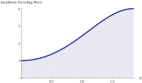
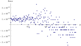
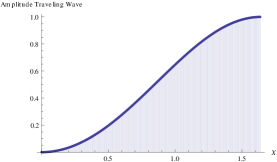
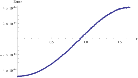
Figure 1. The graphs on the left represent numerically generated, periodic traveling waves of the KdV equation. The graphs on the right represent the difference between the numerical and analytical solutions. The solutions are depicted over half the period.

In the second experiment we attempt to reproduce periodic traveling waves of the Benjamin-Ono equation. We choose $c=-5$, $a=0$, $T=\pi/2$ and we recall from (3.16) or [Ben70], for instance, that

$$u(x;5,0,\pi/2)=\frac{16}{5+3\cos(4x)}$$

solves

$$Hu_{x}=u^{2}+5u,\qquad u(x+\pi/2)=u(x).$$

The results from the numerical experiment are in Figure 2. The agreement between the numerical and analytical solutions is excellent.

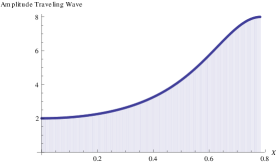
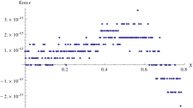
Figure 2. The graph on the left represents the numerically generated, periodic traveling wave of the Benjamin-Ono equation. The graph on the right represents the difference between the numerical and analytical solutions.

We promptly use the numerical routines to explore spectral instability for (3.1) near the origin to long wavelengths perturbations. Specifically we shall numerically implement formulae in Section 3.3. We compute $M$, $P$, $U$ from numerically generated solutions of (3.8) using a trapezoidal rule and numerically differentiate them using a two point symmetric stencil.

In the case of the KdV equation

$$u_{xx}=u^{2}-2u-2,\qquad u(x+2K(\sqrt{2}/2))=u(x),$$

for instance, the effective dispersion matrix in (3.46) is numerically found to be

$${\bf D}=\left(\begin{array}[]{ccc}-17.0603&-70.4702&-4.82493\\ 1&24.4707&0\\ 33.8253&-446.679&29.2956\end{array}\right),$$

whose eigenvalues are $\mu\approx 31.64$, $\mu\approx 14.08$, $\mu\approx-9.016$. Therefore the underlying, periodic traveling wave is modulationally stable, reproducing the known result.

In the case of the Benjamin-Ono equation

$$Hu_{x}=u^{2}-5u,\qquad u(x+\pi/2)=u(x),$$

for instance, the effective dispersion matrix is approximately

$${\bf D}=\left(\begin{array}[]{ccc}-4.9348&8.76682&\text{2.7902947983404674$\grave{}$*${}^{\wedge}$-11}\\ 1&4.9348&0\\ 19.7392&\text{7.435829729729448$\grave{}$*${}^{\wedge}$-10}&4.9348\end{array}\right),$$

whose eigenvalues are $\mu\approx 5.755$, $\mu\approx-5.755$, $\mu\approx 4.935$. Therefore the underlying, periodic traveling wave is modulationally stable. This is in excellent agreement with the results of Section 3.4, where $\mu_{1}=\frac{\pi^{2}\sqrt{34}}{10}\approx 5.755$, $\mu_{2}=-\frac{\pi^{2}\sqrt{34}}{10}\approx-5.755$, $\mu_{3}=\frac{\pi^{2}}{2}\approx 4.935$.

We examined parameter values in the range $1<\alpha<2$ and found, interestingly, a modulationally unstable wave. We chose $c=-5$, $a=0$, $T=\pi/2$ and allowed $\alpha$ to vary between $\alpha\approx.95$ and $\alpha\approx 1.17$. Following the solution branch, below $\alpha\approx.95$ the numerical scheme failed to converge whereas above $\alpha\approx 1.17$ it converged to the constant solution $u=5$. We found that the eigenvalues depended rather sensitively upon the parameter $\alpha$, and the underlying, periodic traveling wave became unstable at $\alpha\approx 1.025$.

The results from the numerical experiment are in Figure 3. The graph on the left side of the figure represents the imaginary part of the eigenvalue as a function of $\alpha$. It is zero for $\alpha\lessapprox 1.025$, implying stability, and increases beyond the exponent. The graph on the right represents the profile of the periodic traveling wave at the onset of instability, $\alpha\approx 1.025$. It seems shallower than the corresponding, periodic traveling wave of the Benjamin-Ono equation. But it seems to arise, though.

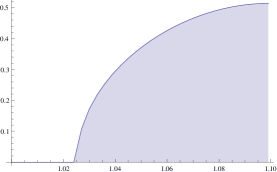
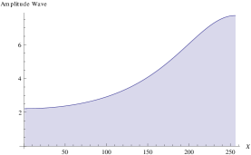
Figure 3. The graph on the left depicts the imaginary part of the eigenvalue as a function of $\alpha$. The graph on the right represents the wave profile at the onset of instability.

The Petviashvili method works reasonably well in general but has a number of drawbacks. For many parameter values, it either fails to converge or converges to the no-wave solution. Furthermore, the convergence of the method is governed by eigenvalues of the associated linearized operator and it is unclear if this somehow biases solutions one sees. It would be interesting to study stability and its transitions for (3.1) (or (1.1)) using a more sophisticated numerical method.

5. Application: general nonlinearities

We shall discuss how the developments in Section 2 and Section 3 may be adapted to the KdV equation with fractional dispersion and the general nonlinearity

(5.1) $$u_{t}-\Lambda^{\alpha}u_{x}+f(u)_{x}=0,$$

where $0<\alpha\leqslant 2$ and $f$ is of $C^{2}$.

Notice that (5.1) possesses three conserved quantities (abusing notation)

(5.2) $$H(u)= \int^{T}_{0}\Big{(}\frac{1}{2}u\Lambda^{\alpha}u-F(u)\Big{)}~{}dx=:K(u)+U(u),$$

where $$F^{\prime}=f$$, and

(5.3) $$P(u)= \int^{T}_{0}\frac{1}{2}u^{2}~{}dx,$$

(5.4) $$M(u)= \int^{T}_{0}u~{}dx.$$

They correspond, respectively, to the Hamiltonian and the momentum, the mass; $K$ and $U$ correspond, respectively, to the kinetic and potential energies. Throughout the section we use $H$, $K$, $U$ and $P$, $M$ for those in (5.2) and (5.3), (5.4).

Clearly (5.1) is in the Hamiltonian form (2.1), for which $J=\partial_{x}$. Notice that $H$, $P$, $M$ are smooth in an appropriate subspace of $H^{\alpha}_{per}([0,T])$ and invariant under spatial translations. Clearly they satisfy (3.6).

Assume that (5.1) admits a smooth, four-parameter family of periodic traveling waves, denoted $u(\cdot+x_{0};c,a,T)$, where $c$ and $a$ form an open set in $\mathbb{R}^{2}$, $x_{0}\in\mathbb{R}$ and $T>0$ are arbitrary, and $u$ is even and $T$-periodic, satisfying by quadrature that

(5.5) $$\Lambda^{\alpha}u-f(u)-cu-a=0$$

(in the sense of distributions), or equivalently (abusing notation)

(5.6) $$\delta E(u;c,a):=\delta(H(u)-cP(u)-aM(u))=0.$$

For a broad range of $\alpha$ and nonlinearities, the existence of periodic traveling waves of (5.1) may follow from variational arguments, e.g., the mountain pass theorem applied to a suitable variational problem whose critical point satisfies (5.5). Assume that a periodic traveling wave $u=u(\cdot+x_{0};c,a,T)$ of (5.1) satisfies Assumption 2.5. We shall address its spectral instability near the origin to long wavelengths perturbations.

In particular we follow the approach in Section 2 and Section 3.3 and we calculate the modulational instability index $\Delta$, defined in (2.31), in terms of inner products between

(5.7a) $$v_{1} =u_{a},\qquad w_{1}=M_{c}u-P_{c},$$

(5.7b) $$v_{2} =u_{x},\qquad w_{2}=\partial_{x}^{-1}(M_{a}u_{c}-M_{c}u_{a}),$$

(5.7c) $$v_{3} =u_{c},\qquad w_{3}=P_{a}-M_{a}u,$$

together with $L_{0}^{-1}$, where

(5.8a) $$L_{0}:= \partial_{x}(\Lambda^{\alpha}-f^{\prime}(u)-c)$$

and

(5.8b) $$L_{1}:= [L_{0},x]=(\alpha+1)\Lambda^{\alpha}-f^{\prime}(u)-c,$$

(5.8c) $$L_{2}:= [L_{1},x]=\alpha(\alpha+1)\Lambda^{\alpha-2}\partial_{x}.$$

We shall ultimately express the index in terms of $K$ and $U$, $P$, $M$, together with their derivatives with respect to $c$, $a$ as well as $\Omega=1/T$. Notice that $v_{j}$’s and $w_{j}$’s satisfy (2.13a)-(2.13c), (2.14) and (2.20).

Below we extend Lemma 3.1 and develop integral identities that a periodic solution of (5.5), or equivalently (5.6), a priori satisfies.

Lemma 5.1.

If $u$ is $T$-periodic and satisfies (5.5) (in the sense of distributions) then

(5.9) $$\int^{T}_{0}f(u)~{}dx\,+\,cM+aT=0,$$

(5.10) $$2K- \int^{T}_{0}uf(u)~{}dx-2cP-aM=0,$$

(5.11) $$(\alpha-1)K- \int^{T}_{0}F(u)~{}dx\,+\,cP+aM+TE_{T}=0.$$

Multiplying (5.5) by $1,u,xu_{x}+Tu_{T}$, respectively, and integrating over the periodic interval $[0,T]$, the proof is similar to that of Lemma 3.1. Hence we omit the detail.

In the case of power-law nonlinearities, $uf(u)$ and $F(u)$ are proportional. Therefore one may relate, e.g., the kinetic energy to the potential energy, the momentum, the mass; see Lemma 3.1. In the case of general nonlinearities, for which scaling invariance is lost, on the other hand, the kinetic and potential energies, the momentum, the mass are no longer linearly dependent. Hence the modulational instability index will depend upon all $K,U,P,M$. Furthermore their derivatives with respect to $c,a,T$ are not linearly dependent. Hence the index will depend upon $K,U,P,M$, together with their derivatives with respect to $c,a,T$.

We promptly rewrite $\langle w_{j},L_{1}v_{k}\rangle$, $j,k=1,2,3$, in terms of $K,U,P,M$ as functions of $c,a,T$. Differentiating (5.10) and (5.9) with respect to $a$ we obtain that

$$2K_{a}+U_{a}-\int^{T}_{0}uf^{\prime}(u)u_{a}~{}dx-2cP_{a}-(aM)_{a}=0\text{ and }\int^{T}_{0}f^{\prime}(u)u_{a}~{}dx+cM_{a}+T=0,$$

respectively. Since $L_{1}$ is self-adjoint and since

$$L_{1}u=(\alpha+1)\Lambda^{\alpha}u-f^{\prime}(u)-cu\quad\text{and}\quad L_{1}1=-f^{\prime}(u)-c,$$

we substitute (5.7a) and calculate that

$$\langle w_{1},L_{1}v_{1}\rangle= \langle L_{1}w_{1},v_{1}\rangle=M_{c}\langle L_{1}u,u_{a}\rangle-P_{c}\langle L_{1}1,u_{a}\rangle$$

$$= M_{c}\Big{(}(\alpha+1)K_{a}-\int^{T}_{0}uf^{\prime}(u)u_{a}~{}dx-cP_{a}\Big{)}-P_{c}\Big{(}-\int^{T}_{0}f^{\prime}(u)u_{a}~{}dx-cM_{a}\Big{)}$$

$$= M_{c}((\alpha-1)K_{a}-U_{a}+cP_{a}+(aM)_{a})-P_{c}T$$

(5.12a) $$= M_{c}(\alpha K_{a}-E_{a})-P_{c}T.$$

The last equality utilizes $$E=K+U-cP-aM$$. Similarly

(5.12b) $$\langle w_{1},L_{1}v_{3}\rangle= \quad\,M_{c}(\alpha K_{c}-E_{c}+P)-P_{c}M,$$

(5.12c) $$\langle w_{3},L_{1}v_{1}\rangle= -M_{a}(\alpha K_{a}-E_{a})+P_{a}T,$$

(5.12d) $$\langle w_{3},L_{1}v_{3}\rangle= -M_{a}(\alpha K_{c}-E_{c}+P)+P_{c}M.$$

Moreover we substitute (5.7b) and make an explicit calculation to obtain that

$$\langle w_{2},L_{1}v_{2}\rangle= \langle\partial_{x}^{-1}(M_{a}u_{c}-M_{c}u_{a}),((\alpha+1)\Lambda^{\alpha}-f^{\prime}(u)-c)u_{x}\rangle$$

$$= \langle\partial_{x}^{-1}(M_{a}u_{c}-M_{c}u_{a}),\partial_{x}((\alpha+1)\Lambda^{\alpha}u-f(u)-cu)\rangle$$

$$= -\langle M_{a}u_{c}-M_{c}u_{a},\,\alpha f(u)+\alpha cu+(\alpha+1)a\rangle$$

(5.13) $$= -\alpha(\{M,U\}_{c,a}-cG).$$

To proceed, differentiating (5.10) and (5.9) with respect to $x\partial_{x}+T\partial_{T}$ leads, with help of (3.14) and (2.35), to that

$$2\alpha K-2(\Omega K)_{\Omega}-(\Omega U)_{\Omega}-\int^{T}_{0}uf^{\prime}(u)(xu_{x}+Tu_{T})~{}dx+2c(\Omega P)_{\Omega}+a(\Omega M)_{\Omega}=0$$

and

$$\int^{T}_{0}f^{\prime}(u)(xu_{x}+Tu_{T})~{}dx-c(\Omega M)_{\Omega}=0,$$

respectively. We then use (2.33) and (3.14), (2.35) to calculate that

$$\langle w_{1}L_{1}L_{0}^{-1}L_{1}v_{2}\rangle= \langle L_{1}w_{1},xu_{x}+Tu_{T}\rangle-G^{-1}\langle w_{1},xu_{x}+Tu_{T}\rangle\langle L_{1}w_{1},v_{1}\rangle$$

$$= M_{c}\langle L_{1}u,xu_{x}+Tu_{T}\rangle-P_{c}\langle L_{1}1,xu_{x}+Tu_{T}\rangle$$

$$-G^{-1}(M_{c}\langle u,xu_{x}+Tu_{T}\rangle-P_{c}\langle 1,xu_{x}+Tu_{T}\rangle)\langle L_{1}w_{1},v_{1}\rangle$$

(5.14a) $$= M_{c}(\alpha(\alpha-1)K-(\Omega(\alpha K-E))_{\Omega})$$

$$-G^{-1}(M_{c}(\Omega P)_{\Omega}-P_{c}(\Omega M)_{\Omega})(M_{c}(\alpha K_{a}-E_{a})-P_{c}T).$$

Similarly

$$\langle w_{3},L_{1}L_{0}^{-1}L_{1}v_{2}\rangle= \langle L_{1}w_{3},xu_{x}+Tu_{T}\rangle-G^{-1}\langle w_{1},xu_{x}+Tu_{T}\rangle\langle L_{1}w_{3},v_{1}\rangle$$

(5.14b) $$= -M_{a}(\alpha(\alpha-1)K-(\Omega(\alpha K-E))_{\Omega})$$

$$+G^{-1}(M_{c}(\Omega P)_{\Omega}-P_{c}(\Omega M)_{\Omega})(M_{a}(\alpha K_{a}-E_{a})-P_{a}T).$$

Note from (5.8c) that

(5.15) $$\langle w_{1},L_{2}v_{2}\rangle=-2\alpha(\alpha+1)M_{c}K\quad\text{and}\quad\langle w_{3},L_{2}v_{2}\rangle=2\alpha(\alpha+1)M_{a}K.$$

To summarize, the effective dispersion matrix, defined in (2.27), is

$${\bf D}=\left(\begin{matrix}0&D_{12}&D_{13}\\ 1&D_{22}&0\\ D_{31}&D_{32}&D_{33}\end{matrix}\right),$$

where, substituting (5.12a)-(5.12d), (5.13) and (5.14a), (5.14b), (5.15) into (2.25b), (2.25c), (2.25e) and (2.25g), (2.25h), (2.25j), we make an explicit calculation to obtain that

$$D_{12}= -2\alpha^{2}GM_{a}K-G(\Omega(\alpha K-E))_{\Omega}$$

$$+M_{c}((\Omega P)_{\Omega}-P_{c}(\Omega M)_{\Omega})(M_{a}(\alpha K_{a}-E_{a})-P_{a}T),$$

$$D_{13}= -M_{a}(\alpha K_{a}-E_{a})+P_{a}T,$$

$$D_{22}= -\alpha(\{M,U\}_{c,a}-cG)-M_{a}(\alpha K_{c}-E_{c}+P)+P_{a}M,$$

$$D_{31}= M_{c}(\alpha K_{c}-E_{c}+P)-P_{c}M,$$

$$D_{32}= 2\alpha^{2}GM_{c}K-G(\Omega(\alpha K-E))_{\Omega}$$

$$-M_{c}(\Omega P)_{\Omega}-P_{c}(\Omega M)_{\Omega})(M_{c}(\alpha K_{a}-E_{a})-P_{c}T)$$

$$+(M_{c}(\alpha K_{c}-E_{c}+P)-P_{c}M)$$

$$\qquad\cdot(\alpha\{M,U\}_{c,a}-cG+M_{a}(\alpha K_{c}-E_{c}+P)+P_{c}M),$$

$$D_{33}= M_{c}(\alpha K_{a}-E_{a})-P_{c}T.$$

Furthermore a complex eigenvalue of ${\bf D}$ implies modulational instability.

Appendix A Proof of Lemma 3.9

We first prove (3.24) in finite dimensions. Suppose that $\vec{e}_{1},\vec{e}_{2},\ldots,\vec{e}_{n}$ form a basis of ${\mathbb{R}}^{n}$ and $\vec{e}_{1},\vec{e}_{2},\ldots,\vec{e}_{k}$ form a basis of $S\subset\mathbb{R}^{n}$. Recall from the Jacobi-Sturm sequence argument that the number of negative eigenvalues of an $n\times n$ matrix ${\bf M}=(m_{ij})_{i,j=1}^{n}$ is equal to the number of sign changes in

$$1,m_{1},m_{2},\ldots,m_{n},$$

where $m_{k}$ is $k$-th principal minor, defined as

$$m_{k}=\det(m_{ij})_{i,j=1}^{k}.$$

The number of negative eigenvalues of ${\bf M}|_{S}$ is, similarly, equal to the number of sign changes in

$$1,m_{1},m_{2},\ldots,m_{k}.$$

Moreover recall from a duality formula for minor determinants that the number of negative eigenvalues of $({\bf M}^{-1})|_{S^{\perp}}$ is

$$1,\frac{m_{n-1}}{m_{n}},\frac{m_{n-2}}{m_{n}},\ldots,\frac{m_{k}}{m_{n}}.$$

Therefore (3.24) follows. (Let $I$ and $J$ be subsets of $\{1,2,\ldots,n\}$ of size $k$, i.e., $|I|=|J|=k$ and let $\det_{I,J}({\bf M})=\det(m_{i,j})_{i\in I,j\in J}$. If $I^{\prime},J^{\prime}$ denote the complementary sets to $I,J$ then

$$\det_{I,J}({\bf M}^{-1})=(-1)^{(\sum_{i\in I}i+\sum_{j\in J}j)}\frac{\det_{J^{\prime},I^{\prime}}({\bf M})}{\det({\bf M})}.$$

To interpret, inverse matrices take $k$-minor determinants to complementary $(n-k)$-minor determinants, like the Hodge-* operator acts on $k$-forms. A proof based upon the Schur complement formula may be found in [Ser10, pp. 41].)

To proceed, let ${\bf M}$ be invertible and bounded below with compact resolvent. Let $\mu_{1}\leqslant\mu_{2}\leqslant\mu_{3}\ldots$ denote eigenvalues of ${\bf M}$, and $v_{1},v_{2},v_{3},\ldots$ be the corresponding eigenvectors. Let $S_{n}$ denote the subspace spanned by $v_{1},v_{2},\ldots,v_{n}$ and let ${\bf M}_{n}=\Pi_{S_{n}}{\bf M}\Pi_{S_{n}}$ denote the symmetric projection of $M$ onto $S_{n}$. Then,

• ${\bf M}_{n}\to{\bf M}$ as $n\to\infty$ in the strong operator topology and $n_{-}({\bf M}_{n})=n_{-}({\bf M})$ for $n$ sufficiently large;

• if ${\bf M}$ is invertible then ${\bf M}_{n}:S_{n}\to S_{n}$ is invertible for $n$ sufficiently large;

• $({\bf M}_{n})^{-1}\to{\bf M}^{-1}$ in the uniform operator topology and $n_{-}(({\bf M}_{n})^{-1}|_{S\perp})=n_{-}({\bf M}^{-1}|_{S^{\perp}})$ for $n$ sufficiently large;

• ${\bf M}|_{S}={\bf M}_{n}|_{S}$.

Therefore (3.24) follows from a limiting argument.

Acknowledgements

JCB is supported by the National Science Foundation under grant No. DMS–1211364 and by a Simons Foundation fellowship. He would like to thank the Department of Mathematics at MIT for its hospitality during the writing of the paper. VMH is supported by the National Science Foundation under grant No. DMS–1008885, the University of Illinois at Urbana-Champaign under the Campus Research Board grant No. 11162 and by an Alfred P. Sloan research fellowship.

References

• [AL84] D Anderson and M Lisak, Modulational instability of coherent optical-fiber transmission signals, Opt. Lett. 9 (1984), no. 10, 468–470.
• [APN08] Jaime Angulo Pava and Fábio M. A. Natali, Positivity properties of the Fourier transform and the stability of periodic travelling-wave solutions, SIAM J. Math. Anal. 40 (2008), no. 3, 1123–1151. MR 2452883 (2009i:35262)
• [AT91] C. J. Amick and J. F. Toland, Uniqueness and related analytic properties for the Benjamin-Ono equation—a nonlinear Neumann problem in the plane, Acta Math. 167 (1991), no. 1-2, 107–126. MR 1111746 (92i:35099)
• [BBM72] T. B. Benjamin, J. L. Bona, and J. J. Mahony, Model equations for long waves in nonlinear dispersive systems, Philos. Trans. Roy. Soc. London Ser. A 272 (1972), no. 1220, 47–78. MR 0427868 (55 #898)
• [BD09] Nate Bottman and Bernard Deconinck, KdV cnoidal waves are spectrally stable, Discrete Contin. Dyn. Syst. 25 (2009), no. 4, 1163–1180. MR 2552133 (2011h:35239)
• [Ben70] T. Brooke Benjamin, Internal waves of permanent form in fluids of great depth, Journal of Fluid Mechanics 29 (1970), no. 3, 559–592.
• [BF67] T. Brooke Benjamin and J. E. Feir, The disintegration of wave trains on deep water. Part 1. Theory, J. Fluid Mech. 27 (1967), no. 3, 417–437.
• [BJ10] Jared C. Bronski and Mathew A. Johnson, The modulational instability for a generalized Korteweg-de Vries equation, Arch. Ration. Mech. Anal. 197 (2010), no. 2, 357–400. MR 2660515 (2012f:35456)
• [BM95] Thomas J. Bridges and Alexander Mielke, A proof of the Benjamin-Feir instability, Arch. Rational Mech. Anal. 133 (1995), no. 2, 145–198. MR 1367360 (97c:76028)
• [BN67] D. J. Benney and A. C. Newell, The propagation of nonlinear wave envelopes, J. Math. and Phys. 46 (1967), 133–139. MR 0241052 (39 #2397)
• [Bou77] M. J Boussinesq, Essai sur la théorie des eaux courants, Mémoirs présentés par divers savants á l’Acad. des Sciences Inst. France (série 2) 23 (1877), 1–680.
• [BSS87] J. L. Bona, P. E. Souganidis, and W. A. Strauss, Stability and instability of solitary waves of Korteweg-de Vries type, Proc. Roy. Soc. London Ser. A 411 (1987), no. 1841, 395–412. MR 897729 (88m:35128)
• [CDLFM07] P. Cardaliaguet, F. Da Lio, N. Forcadel, and R. Monneau, Dislocation dynamics: a non-local moving boundary, Free boundary problems, Internat. Ser. Numer. Math., vol. 154, Birkhäuser, Basel, 2007, pp. 125–135. MR 2305351 (2007m:74025)
• [Chi06] Carmen Chicone, Ordinary differential equations with applications, second ed., Texts in Applied Mathematics, vol. 34, Springer, New York, 2006. MR 2224508 (2006m:34001)
• [CPV05] Scipio Cuccagna, Dmitry Pelinovsky, and Vitali Vougalter, Spectra of positive and negative energies in the linearized NLS problem, Comm. Pure Appl. Math. 58 (2005), no. 1, 1–29. MR 2094265 (2005k:35374)
• [CT04] Rama Cont and Peter Tankov, Financial modelling with jump processes, Chapman & Hall/CRC Financial Mathematics Series, Chapman & Hall/CRC, Boca Raton, FL, 2004. MR 2042661 (2004m:91004)
• [DS09] Wolf-Patrick Düll and Guido Schneider, Validity of Whitham’s equations for the modulation of periodic traveling waves in the NLS equation, J. Nonlinear Sci. 19 (2009), no. 5, 453–466. MR 2540165 (2011c:35532)
• [FL12] Rupert Frank and Enno Lenzmann, Uniqueness and nondegeneracy of ground states for $(-{\Delta})^{2}{Q}+{Q}-{Q}^{\alpha+1}=0$ in $\mathbb{R}$, Acta Math. (2012), to appear.
• [FPU55] Enrico Fermi, J. Pasta, and S. Ulam, Studies of nonlinear problems, Los Alamos Scientific Laboratory (1955), no. LA-1940.
• [GLM07] Fritz Gesztesy, Yuri Latushkin, and Konstantin A. Makarov, Evans functions, Jost functions, and Fredholm determinants, Arch. Ration. Mech. Anal. 186 (2007), no. 3, 361–421. MR 2350362 (2008k:34209)
• [GLZ08] Fritz Gesztesy, Yuri Latushkin, and Kevin Zumbrun, Derivatives of (modified) Fredholm determinants and stability of standing and traveling waves, J. Math. Pures Appl. (9) 90 (2008), no. 2, 160–200. MR 2437809 (2012b:47035)
• [GSS87] Manoussos Grillakis, Jalal Shatah, and Walter Strauss, Stability theory of solitary waves in the presence of symmetry. I, J. Funct. Anal. 74 (1987), no. 1, 160–197. MR 901236 (88g:35169)
• [Has72] Akira Hasegawa, Theory and computer experiment on self-trapping instability of plasma cyclotron waves, Physics of Fluids 15 (1972), no. 5, 870–881.
• [Hay68] Emilie V. Haynsworth, Determination of the inertia of a partitioned Hermitian matrix, Linear Algebra and Appl. 1 (1968), no. 1, 73–81. MR 0223392 (36 #6440)
• [HJ12] Vera Mikyoung Hur and Mathew A. Johnson, Stability of periodic traveling waves for nonlinear dispersive equations, SIAM J. Math. Anal. (2012), preprint.
• [HK95] Akira Hasegawa and Yuji Kodama, Solitons in optical communications, Clarendon Press, Oxford, 1995.
• [Hur12] Vera Mikyoung Hur, On the formation of singularities for surface water waves, Commun. Pure Appl. Anal. 11 (2012), no. 4, 1465–1474. MR 2900797
• [Jos77] R. I. Joseph, Solitary waves in a finite depth fluid, J. Phys. A 10 (1977), no. 12, 225–227. MR 0455822 (56 #14056)
• [JZ10] M. A. Johnson and K. Zumbrun, Rigorous justification of the Whitham modulation equations for the generalized Korteweg-de Vries equation, Stud. Appl. Math. 125 (2010), no. 1, 69–89. MR 2676781 (2011h:35249)
• [KdV95] D Korteweg and G. de Vries, On the change of form of long waves advancing in a rectangular canal, and on a new type of long stationary waves, Phil. Mag. 39 (1895), 422–443.
• [KMR11] C. E. Kenig, Y. Martel, and L. Robbiano, Local well-posedness and blow-up in the energy space for a class of $L^{2}$ critical dispersion generalized Benjamin-Ono equations, Ann. Inst. H. Poincaré Anal. Non Linéaire 28 (2011), no. 6, 853–887. MR 2859931
• [KP12] Todd Kapitula and Keith Promislow, Stability indices for constrained self-adjoint operators, Proc. Amer. Math. Soc. 140 (2012), no. 3, 865–880. MR 2869071
• [Kwo89] Man Kam Kwong, Uniqueness of positive solutions of $\Delta u-u+u^{p}=0$ in ${\bf R}^{n}$, Arch. Rational Mech. Anal. 105 (1989), no. 3, 243–266. MR 969899 (90d:35015)
• [Lig65] M. J. Lighthill, Contributions to the theory of waves in non-linear dispersive systems, IMA J. Appl. Math. 1 (1965), no. 3, 269–306.
• [Lin08] Zhiwu Lin, Instability of nonlinear dispersive solitary waves, J. Funct. Anal. 255 (2008), no. 5, 1191–1224. MR 2455496 (2010m:35456)
• [LY07] T. I. Lakoba and J. Yang, A mode elimination technique to improve convergence of iteration methods for finding solitary waves, J. Comput. Phys. 226 (2007), no. 2, 1693–1709. MR 2356391 (2008j:35055)
• [MB89] C. J. McKinstrie and R. Bingham, The modulational instability of coupled waves, Physics of Fluids B 1 (1989), 230–237.
• [New85] Alan C. Newell, Solitons in mathematics and physics, CBMS-NSF Regional Conference Series in Applied Mathematics, vol. 48, Society for Industrial and Applied Mathematics (SIAM), Philadelphia, PA, 1985. MR 847245 (87h:35314)
• [Ono75] Hiroaki Ono, Algebraic solitary waves in stratified fluids, J. Phys. Soc. Japan 39 (1975), no. 4, 1082–1091. MR 0398275 (53 #2129)
• [Ost67] L. A. Ostrovsky, Propagation of wave packets in nonlinear dispersive medium, Sov. J. Exp. Theor. Phys. 24 (1967), 797–800.
• [OZ03a] M. Oh and K. Zumbrun, Stability of periodic solutions of conservation laws with viscosity: analysis of the Evans function, Arch. Ration. Mech. Anal. 166 (2003), no. 2, 99–166. MR 1957127 (2004c:35270a)
• [OZ03b] by same author, Stability of periodic solutions of conservation laws with viscosity: pointwise bounds on the Green function, Arch. Ration. Mech. Anal. 166 (2003), no. 2, 167–196. MR 1957128 (2004c:35270b)
• [Pet76] V.I. Petviashvili, Equation for an extraordinary soliton, Sov. J. Plasma Phys. 2 (1976), 469–472.
• [PW92] Robert L. Pego and Michael I. Weinstein, Eigenvalues, and instabilities of solitary waves, Philos. Trans. Roy. Soc. London Ser. A 340 (1992), no. 1656, 47–94. MR 1177566 (93g:35115)
• [Ser05] Denis Serre, Spectral stability of periodic solutions of viscous conservation laws: large wavelength analysis, Comm. Partial Differential Equations 30 (2005), no. 1-3, 259–282. MR 2131054 (2006f:35178)
• [Ser10] by same author, Matrices, second ed., Graduate Texts in Mathematics, vol. 216, Springer, New York, 2010, Theory and applications. MR 2744852 (2011i:15001)
• [THT86] K. Tai, A. Hasegawa, and A. Tomita, Observation of modulational instability in optical fibers, Phys. Rev. Lett. 56 (1986), no. 2, 135–138.
• [Wei87] Michael I. Weinstein, Existence and dynamic stability of solitary wave solutions of equations arising in long wave propagation, Comm. Partial Differential Equations 12 (1987), no. 10, 1133–1173. MR 886343 (88h:35107)
• [Whi67] G. B. Whitham, Non-linear dispersion of water waves, J. Fluid Mech. 27 (1967), 399–412. MR 0208903 (34 #8711)
• [Whi74] by same author, Linear and nonlinear waves, Pure and Applied Mathematics (New York), Wiley-Interscience [John Wiley & Sons], New York, 1974. MR 0483954 (58 #3905)
• [YL08] Jianke Yang and Taras I. Lakoba, Accelerated imaginary-time evolution methods for the computation of solitary waves, Stud. Appl. Math. 120 (2008), no. 3, 265–292. MR 2406821 (2009c:35447)
• [Zak68a] V. E. Zakharov, Instability of self-focusing of light, Sov. J. Exp. Theor. Phys. 26 (1968), 994.
• [Zak68b] by same author, Stability of periodic waves of finite amplitude on the surface of a deep fluid, J. Appl. Mech. Tech. Phys. 9 (1968), no. 2, 190–194.