RUNHETC-2013-06

ODE/IM correspondence for the Fateev model

Sergei L. Lukyanov^1,2

¹NHETC, Department of Physics and Astronomy

Rutgers University

Piscataway, NJ 08855-0849, USA

and

²L.D. Landau Institute for Theoretical Physics

Chernogolovka, 142432, Russia

Dedicated to my PhD advisor V.A. Fateev on the occasion of his 65th anniversary

Abstract

The Fateev model is somewhat special among two-dimensional quantum field theories. For different values of the parameters, it can be reduced to a variety of integrable systems. An incomplete list of the reductions includes $O(3)$ and $O(4)$ non-linear sigma models and their continuous deformations (2D and 3D sausages, anisotropic principal chiral field), the Bukhvostov-Lipatov model, the $N=2$ supersymmetric sine-Gordon model, as well as the integrable perturbed $SU_{2}(n)\otimes SU_{2}(p-2)/SU_{2}(n+p-2)$ coset CFT. The model possesses a mysterious symmetry structure of the exceptional quantum superalgebras $U_{q}{\widehat{\big{(}D(2|1;\alpha)}}\big{)}$.

In this work, we propose the ODE/IM correspondence between the Fateev model and a certain generalization of the classical problem of constant mean curvature embedding of a thrice-punctured sphere in $AdS_{3}$.

 

March 2013

1 Introduction

Broadly speaking the ODE/IM correspondence is a link between the theory of Integrable Models in two dimensions and the spectral analysis of Ordinary Differential Equations. The approach was originated by Dorey and Tateo in Ref.[1] from the observation that the thermodynamic Bethe ansatz equations for certain 2D CFT minimal models proposed in [2] coincide with an exact version of the Bohr-Sommerfeld quantization condition for 1D anharmonic oscillator – a remarkable result due to Voros [3, 4, 5]. Very shortly the initial observation was generalized and proved in Ref.[6]. Later the ODE/IM correspondence was established for a large variety of models (for review see [7]). However, during the next decade, all attempts to incorporate massive integrable QFT in the ODE/IM correspondence have failed. Since the work of Gaiotto, Moore and Neitzke [8], thermodynamic Bethe ansatz equations have emerged in different contexts of SUSY gauge theories, algebraic and differential geometry [9, 10, 11, 12]. Inspired by this progress Zamolodchikov and the author have established the ODE/IM correspondence for the quantum sine/sinh-Gordon model – the model which always served as a basis for the development of the 2D integrable QFT [13]. Recently the result of Ref.[13] was extended to the Toda type QFT model [14]. It has become clear that the ODE/IM correspondence is one of the most important aspects of integrability in 2D QFT. Among open problems within the approach is how to incorporate the class of integrable non linear sigma models into the ODE/IM correspondence. In this work, we propose an example which aims to step in this direction.

We begin with the following well known fact (see e.g. Ref.[15]); Let $\Sigma_{g,n}$ be a compact Riemann surface with $n$ marked points (“punctures”) and $a_{1},\,a_{2},\ldots a_{n}$ be positive numbers such that $2\,\chi(\Sigma_{g})+\sum_{i=1}^{n}(a_{i}-2)=0$. Then there exists a flat metric on $\Sigma_{g,n}$ with conical singularities of angle $\pi a_{i}$ at the ${i}^{{\rm th}}$ puncture. The metric is unique up to homothety.

In the case of a two-sphere with three punctures the theorem’s condition reads as

$$a_{1}+a_{2}+a_{3}=2\ ,$$ (1.1)

whereas its statement is somewhat trivial. Indeed introduce a complex coordinate $z$ and define a holomorphic differential $p(z)\,(\mbox{d}z)^{2}$ on the universal cover of $\Sigma_{0,3}$ by means of the following assignment for $p(z)$:

$$p(z)=\rho^{2}\ \frac{(z_{3}-z_{2})^{a_{1}}\,(z_{1}-z_{3})^{a_{2}}\,(z_{2}-z_{1})^{a_{3}}}{(z-z_{1})^{2-a_{1}}(z-z_{2})^{2-a_{2}}(z-z_{3})^{2-a_{3}}}\ .$$ (1.2)

Then the flat metric reads explicitly

$$(\mbox{d}s)^{2}_{0}=\sqrt{p(z){\bar{p}}({\bar{z}})}\ {\mbox{d}z}{\mbox{d}{\bar{z}}}\ .$$ (1.3)

Here $\rho$ stands for the homothety parameter and $z_{i}$ labels the punctures.

Consider now the problem of constant mean curvature embedding of $\Sigma_{0,3}$ into $AdS_{3}$. In this case, the Gauss-Peterson-Codazzi equation can be brought to the form of the modified Sinh-Gordon (MShG) equation

$$\partial_{z}\partial_{\bar{z}}{\eta}-\mbox{e}^{2{\eta}}+p(z){\bar{p}}({\bar{z}})\,\mbox{e}^{-2{\eta}}=0\ ,$$ (1.4)

where the field $\eta$ defines the induced metric [16, 17, 18, 10]

$$(\mbox{d}s)^{2}_{\rm cmc}=\frac{4}{1+H^{2}}\ \frac{\mbox{e}^{2\eta}}{\sqrt{p(z){\bar{p}}({\bar{z}})}}\ (\mbox{d}s)^{2}_{0}\ ,$$ (1.5)

and $H=const$ stands for the mean curvature. A suitable solution should be real and smooth as $z\not=z_{i}$, and, if we want to preserve the amount of the Gaussian curvature localized at the punctures, it should satisfy the conditions

$$\eta-{\textstyle\frac{1}{4}}\ \log\big{(}\,p(z){\bar{p}}({\bar{z}})\,)=O(1)\ \ \ \ \ \ {\rm at}\ \ \ z\to z_{i}\ \ (i=1,2,3)\ \ {\rm and}\ \infty\ .$$ (1.6)

It turns out that the problem (1.4), (1.6) admits an important generalization. One can consider the MShG equation in the flat background of the punctured sphere $\Sigma_{0,3}$ subject of more general asymptotic conditions

$$\eta = -2\,\log|z|+O(1)\ \ \ \ \ \ \ \ \ \ \ \ \ \ \ {\rm at}\ \ \ \ \ \ z\to\infty$$

$$\eta = 2m_{i}\,\log|z-z_{i}|+O(1)\ \ \ \ \ \ \ \ {\rm at}\ \ \ \ \ \ z\to z_{i}\ .$$ (1.7)

If

$$0<a_{i}<2$$ (1.8)

and

$$-\frac{1}{2}<m_{i}\leq-\frac{1}{4}\ (2-a_{i})\ ,$$ (1.9)

then the solution of the generalized problem exists and is unique. We are not going to prove this statement here. Instead, we will accept it and argue that the solution of (1.4), (1) is related to a certain 2D integrable QFT model, where all the parameters $a_{i}$, $\rho$ and $m_{i}$, as well as the restrictions (1.8) and (1.9), admit simple physical interpretations.

To describe the relation between classical and quantum systems we shall need an important property of the problem (1.4), (1). The essential point in the formal theory of the equation (1.4) is an existence of an infinite hierarchy of one-forms, which are closed by virtue of the MShG equation only,

$$\{\omega_{2n}\}_{n=1}^{\infty}\ :\ \ \ \ \ \ \ \ \ \ \ \ \ \mbox{d}\omega_{2n}=0\ .$$ (1.10)

They are usually normalized by the condition

$$\omega_{2n}=\Big{(}\,\big{(}\sqrt{p(z)}\,\big{)}^{1-2n}\,(\partial_{z}\eta)^{2n}+\ldots\,\Big{)}\,\mbox{d}z+\big{(}\,\ldots\,\big{)}\ \mbox{d}{\bar{z}}\ ,$$ (1.11)

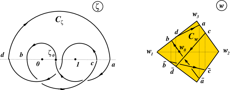
where dots in the first bracket involves terms with higher derivatives of $\partial_{z}\eta$ and/or $p(z)$. The one-forms are not single-valued on the punctured sphere and should be considered on the universal cover of $\Sigma_{0,3}$ caused by the presence of the multivalued function $\sqrt{p(z)}$. However, the contour $C$ depicted in Fig.1, loops around each puncture and $\sqrt{p(z)}$ acquires the same value after the analytic continuation along $C$.

Figure 1: The integration contour $C$ for the conserved charges ${\mathfrak{q}}_{2n-1}$.

Therefore the restriction of $\omega_{2n}$ to $C$ are single-valued and the integrals

$${\mathfrak{q}}_{2n-1}=\oint_{C}\omega_{2n}$$ (1.12)

are not sensitive to continuous deformations of the contour. A branch of multivalued function $\sqrt{p(z)}$ can be chosen in such a way that the conserved charges are real numbers,

$${\mathfrak{q}}_{2n-1}={\mathfrak{q}}^{*}_{2n-1}\ .$$ (1.13)

We now turn to the QFT model of our interest. It was introduced by Fateev in Ref.[19] and governed by the following Lagrangian in the $1+1$ Minkowski space

$${\cal L} = \frac{1}{16\pi}\ \sum_{i=1}^{3}\big{(}\,(\partial_{t}\varphi_{i})^{2}-(\partial_{x}\varphi_{i})^{2}\,\big{)}$$

$$+ 2\mu\ \big{(}\,\mbox{e}^{{\rm i}\,\alpha_{3}\varphi_{3}}\ \cos(\alpha_{1}\varphi_{1}+\alpha_{2}\varphi_{2})+\mbox{e}^{-{\rm i}\alpha_{3}\varphi_{3}}\ \cos(\alpha_{1}\varphi_{1}-\alpha_{2}\varphi_{2})\,\big{)}\,.$$

Here $\alpha_{i}$ are coupling constants subject to a single constraint

$$\alpha_{1}^{2}+\alpha_{2}^{2}+\alpha_{3}^{2}=\frac{1}{2}\ .$$ (1.15)

In this paper, we shall focus on the case where

$$\alpha_{1}^{2}>0\,,\ \ \ \ \ \ \ \alpha_{2}^{2}>0\,,\ \ \ \ \ \ \ \alpha_{3}^{2}>0\,\ .$$ (1.16)

The parameter $\mu$ in the Lagrangian sets the mass scale, $\mu\sim[\,{\rm mass}\,]$. We shall consider the theory in finite-size geometry, with the spatial coordinate $x$ in $\varphi_{i}=\varphi_{i}(x,t)$ compactified on a circle of circumference $R$, with the periodic boundary conditions

$$\varphi_{i}(x+R,t)=\varphi_{i}(x,t)\ .$$ (1.17)

Due to the periodicity of the potential term in (1) in $\varphi_{i}$, the space of states ${\cal H}$ splits on the orthogonal subspaces ${\cal H}_{k_{1},k_{2},k_{3}}$ characterized by the three “quasimomentums” $k_{i}$:

$$\varphi_{i}\to\varphi_{i}+2\pi/\alpha_{i}\ :\ \ \ |\,\Psi_{k_{1},k_{2},k_{3}}\,\rangle\to\mbox{e}^{2\pi{\rm i}k_{i}}\ |\,\Psi_{k_{1},k_{2},k_{3}}\,\rangle\ .$$ (1.18)

The QFT (1) is integrable, in particular it has infinite set of commuting local integrals of motion $\mathbb{I}^{(+)}_{2n-1}$, $\mathbb{I}^{(-)}_{2n-1}$, $2n=2,\,4,\,6,\,\ldots$ being the Lorentz spins of the associated local densities [19]:

$$\mathbb{I}^{(\pm)}_{2n-1}=\int_{0}^{R}\frac{\mbox{d}x}{2\pi}\ \ \Big{[}\,\sum_{i+j+k=n}C^{(n)}_{ijk}\ (\partial_{\pm}\varphi_{1})^{2i}\,(\partial_{\pm}\varphi_{2})^{2j}\,(\partial_{\pm}\varphi_{3})^{2k}+\ldots\,\Big{]}\ ,$$ (1.19)

where $\partial_{\pm}=\frac{1}{2}(\partial_{x}\mp\partial_{t})$ and $\ldots$ stand for the terms involving higher derivatives of $\varphi_{i}$, as well as the terms proportional to powers of $\mu$. The constant $C^{(n)}_{ijk}$ was found in Ref.[20]

$$C^{(n)}_{ijk}=\frac{n!}{i!\ j!\ k!}\ \ \frac{\big{(}2\alpha_{1}^{2}(1-2n)\big{)}_{n-i}\big{(}2\alpha_{2}^{2}\,(1-2n)\big{)}_{n-j}\,\big{(}2\alpha_{3}^{2}\,(1-2n)\big{)}_{n-k}}{(2n-1)^{3}\ (4\alpha^{2}_{1})^{1-i}\ (4\alpha^{2}_{2})^{1-j}\ (4\alpha^{2}_{3})^{1-k}}\ ,$$ (1.20)

where $(x)_{n}$ stands for the Pochhammer symbol. Notice that the displayed terms in (1.19) with the given $C^{(n)}_{ijk}$ set the normalization of $\mathbb{I}^{(\pm)}_{2n-1}$ unambiguously.

Of primary interest are the $k$-vacuum eigenvalues

$$I_{2n-1}=I^{(+)}_{2n-1}(\{k_{i}\}\,|\,R)={I}^{(-)}_{2n-1}(\{k_{i}\}\,|\,R)\ ,$$ (1.21)

especially the $k$-vacuum energy

$$E=2\ I_{1}\ .$$ (1.22)

In the large-$R$ limit all vacuum eigenvalues $I_{2n-1}$ vanish except $I_{1}$. The vacuum energy is composed of an extensive part proportional to the length of the system,

$$E=R\,{\cal E}_{0}+o(1)\ \ \ \ \ \ \ \ \ {\rm at}\ \ \ R\to\infty\ .$$ (1.23)

One of Fateev’s impressive results concerning theory (1) is an elegant analytical expression for the specific bulk energy

$${\cal E}_{0}=-\pi\mu^{2}\ \prod_{i=1}^{3}\frac{\Gamma(2\alpha_{i}^{2})}{\Gamma(1-2\alpha_{i}^{2})}\ .$$ (1.24)

The main observation of this work is that the vacuum eigenvalues can be expressed in terms of the classical conserved charges (1.12):

$$\mu^{-1}\ \big{(}\,I_{1}-{\textstyle\frac{1}{2}}\,R\,{\cal E}_{0}\,\big{)} = d_{1}\ {\mathfrak{q}}_{1}$$ (1.25)

$$\mu^{1-2n}\ I_{2n-1} = d_{n}\ {\mathfrak{q}}_{2n-1}\ \ \ \ \ \ \ \ \ \ \ \ \ \ (n=2,\,3,\,\ldots)\ .$$

Here $d_{n}$ are constants, independent of $k_{i}$ and $R$. With the normalization conditions for ${\mathfrak{q}}_{2n-1}$ and ${\mathbb{I}}^{(\pm)}_{2n-1}$ described above, $d_{n}$ reads explicitly as

$$d_{n}=(2\pi)^{2n-1}\ \ \frac{(-1)^{n-1}}{16\,\pi^{2}}\ \ \prod_{i=1}^{3}\Gamma\big{(}\,2\,(2n-1)\,\alpha^{2}_{i}\,\big{)}\ .$$ (1.26)

The parameters of the quantum and classical problems are identified as follows:

$$\alpha_{i}^{2} = {\frac{a_{i}}{4}}\ \ \ \ \ \ \ \ \ (i=1,2,3)$$

$$|k_{i}| = \frac{1}{a_{i}}\ (2m_{i}+1)\ ,$$ (1.27)

whereas the relation between dimensionless parameter $\mu R$ and $\rho$ is given by

$$\mu R=2\rho\ .$$ (1.28)

Notice that the quantum integrals of motion $\mathbb{I}^{(\pm)}_{2n-1}$ are periodic functions of the quasimomentums, and one can assume that $k_{i}$ takes values within the first Brillouin zone

$$-\frac{1}{2}<k_{i}\leq\frac{1}{2}\ .$$ (1.29)

Since $\mathbb{I}^{(\pm)}_{2n-1}$ commute with the “charge conjugations” – the obvious symmetries $\varphi_{i}\to-\varphi_{i}\ (i=1,2,3)$ of the Lagrangian, the eigenvalues (1.21) are even functions of $k_{i}$. In a view of the identification (1), the inequality (1.29) suggests a natural domain (1.9) for the parameters $m_{i}$. Although both the classical conserved charges and the eigenvalues $I_{2n-1}$ are nonsingular at $k_{i}=0\ (m_{i}=-\frac{1}{2}$), the small-$|z-z_{i}|$ asymptotic (1) contains a subleading $\log\log$-term in this case (the so-called “parabolic point”). For this reason, the value $m_{i}=-\frac{1}{2}$ is excluded from the domain (1.9).

Let us recall now that the MShG equation constitutes a flatness condition for a certain $sl(2)$-valued connection ${\boldsymbol{A}}={\boldsymbol{A}}_{z}\mbox{d}z+{\boldsymbol{A}}_{\bar{z}}\mbox{d}{\bar{z}}$. The associated linear problem

$$(\partial_{z}-{\boldsymbol{A}}_{z})\,{\boldsymbol{\Psi}}=0\ ,\ \ \ \ \ \ \ \ \ \ \ (\partial_{\bar{z}}-{\boldsymbol{A}}_{\bar{z}})\,{\boldsymbol{\Psi}}=0$$ (1.30)

is of prime importance for solving (1.4), (1). In particular, certain monodromy coefficients for the linear system (1.30) can be regarded as generating functions for the set of conserved charges $\{{\mathfrak{q}}_{2n-1}\}_{n=1}^{\infty}$. Thus Eqs.(1.25) relate spectral characteristics of the linear problem (1.30) with a vacuum spectrum of the local integral of motions from the Fateev model. This is an example of the ODE/IM correspondence.

Al.B. Zamolodchikov was probably the first who realized the main advantages of ODE/IM correspondence compare to the traditional approaches [21]; The ODE counterpart makes explicit the analytic properties of relevant physical quantities considered as functions of the parameters. Within the ODE/IM approach, the integrable model can be studied uniformly in different parameter regimes. In the case of massive QFT, this was explicitly demonstrated in Ref.[13] for the quantum sine- and sinh-Gordon models. In spite of formal similarity of the Lagrangians, the physical content of these models is very different from one another. However, the models can be treated uniformly within the ODE/IM approach. With only a few minor modifications one can jump from the trigonometric to the hyperbolic model. The story is repeating itself – only little modifications $\grave{\rm a}$ la sin/sinh-Gordon one are required to extend the above ODE/IM correspondence to the most interesting regime of QFT (1) with

$$\alpha_{1}^{2}>0\,,\ \ \ \ \ \ \ \alpha_{2}^{2}>0\,,\ \ \ \ \ \ \ \alpha_{3}^{2}<0\,.$$ (1.31)

In this regime, the Fateev model provides a dual description of the “3D-sausage” – the integrable non-linear sigma model with three dimensional target space [19]. The sigma-model regime will be the subject of a separate publication. The main purpose of this work is to present evidences in support of the relations (1.25)-(1.28) in the regime (1.16).

The paper is organized as follows. In Section 2 we give an accurate definition of the conserved charges ${\mathfrak{q}}_{2n-1}$ and recall their relation to the flat connection. In the next section we focus on the first conserved charge ${\mathfrak{q}}_{1}$. Our analysis is based on the observation that as $\rho\to 0$ the problem (1.4), (1) is reduced to the problem of constructing a metric of constant intrinsic curvature on the punctured sphere. Using the results from the classical Liouville theory we derive the small-$\rho$ expansion of ${\mathfrak{q}}_{1}$. Section 4 deals with the $\rho\to 0$ limit of the conserved charges ${\mathfrak{q}}_{2n-1}$ with $n>1$. Finally, in Section 5 we extract the relations (1.25)-(1.28) from the comparison of the small-$\rho$ expansions for ${\mathfrak{q}}_{2n-1}$ against predictions of the Conformal Perturbation Theory for the QFT (1). We conclude with a few remarks on a rigorous proof of the proposed ODE/IM correspondence.

In the theory of integrable models, an important r${\hat{\rm o}}$le belongs to the concept of the Yang-Yang function(al) [22]. It is of prime interest to the ODE/IM correspondence [23]. In this work, we use the Yang-Yang function as an auxiliary tool only to derive the small $\rho$-expansion of the conserved charge ${\mathfrak{q}}_{1}$. Because of its own significance, we present some facts concerning the Yang-Yang function for the Fateev model in the appendix.

2 Conserved charges for MShG on the punctured sphere

In this section we give detailed description of the conserved charges $\{{\mathfrak{q}}_{2n-1}\}_{n=1}^{\infty}$.

2.1 From MShG to ShG

The flat metric defines a complex structure on a punctured sphere $\Sigma_{0,3}$. Since the MShG equation (1.4) is covariant under coordinate diffeomorphisms, its form can be simplified by taking advantage of conformal transformations. First of all, we can use the Möbius transformation

$$\zeta=\frac{(z_{2}-z_{3})(z-z_{1})}{(z_{2}-z_{1})(z-z_{3})}$$ (2.1)

to convert the puncture’s coordinates $(z_{1},z_{2},z_{3})$ to their standard values $(0,1,\infty)$. This brings Eq.(1.4) to the form

$$\partial_{\zeta}\partial_{\bar{\zeta}}{\tilde{\eta}}-\mbox{e}^{2{\tilde{\eta}}}+{P}(\zeta){\bar{P}}({\bar{\zeta}})\,\mbox{e}^{-2{\tilde{\eta}}}=0\ ,$$ (2.2)

where

$${\tilde{\eta}}={\eta}+\frac{1}{2}\ \log\Big{(}\frac{\mbox{d}z}{\mbox{d}\zeta}\,\frac{\mbox{d}{\bar{z}}}{\mbox{d}{\bar{\zeta}}}\Big{)}\ ,\ \ \ \ \ \ {P}(\zeta)=\rho^{2}\ \zeta^{a_{1}-2}\ (1-\zeta)^{a_{2}-2}\ .$$ (2.3)

Then we consider the Schwarz-Christoffel mapping

$$w(\zeta)=\int\mbox{d}\zeta\ \sqrt{P(\zeta)}\ ,$$ (2.4)

which transforms the upper half plane $\Im m(\zeta)\geq 0$ to the triangle $(w_{1},\,w_{2},\,w_{3})$ in the complex $w$-plane (see Fig. 2).

Figure 2: Triangle $(w_{1},w_{2},w_{3})$ is a $w$-image of the upper half plane $\Im m(\zeta)>0$ under the Schwarz-Christoffel mapping (2.4). The point ${\bar{w}}_{3}$ is a reflection of $w_{3}$ w.r.t. the straight line $(w_{1},w_{2})$. The domain ${\mathbb{D}}$ is obtained from the 4-polygon $(w_{1},w_{3},w_{2},{\bar{w}}_{3})$ by the identification of the sides $[w_{1},w_{3}]$, $[w_{2},w_{3}]$ and $[w_{1},{\bar{w}}_{3}]$, $[w_{2},{\bar{w}}_{3}]$, respectively.

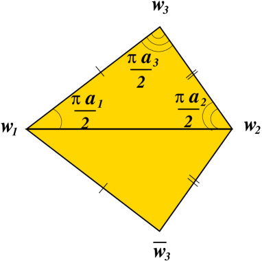
The lower half plane $\Im m(\zeta)\leq 0$ can be mapped into the triangle reflected w.r.t. the straight line $(w_{1},w_{2})$. If there exists a unique solution, it should respect all symmetries of the problem under consideration. In particular it should be invariant under the reflection $\zeta\leftrightarrow{\bar{\zeta}}$:

$${\tilde{\eta}}(\zeta,{\bar{\zeta}})={\tilde{\eta}}({\bar{\zeta}},\zeta)\ .$$ (2.5)

Let ${\mathbb{D}}$ be a four-sided polygon with the vertexes located at $w_{i}=\{w_{1},\,w_{2},\,w_{3},\,{\bar{w}}_{3}\}$ whose adjacent sides are glued together as it is shown in Fig. 2 to form a topological two-sphere. The overall scale of the polygon is governed by the homothety parameter $\rho$ in Eq.(1.2). Without loss of generality we shall assume that $\rho>0$, then

$$|w_{i}-w_{j}|=\rho\ \ \frac{\Gamma(\frac{a_{i}}{2})\Gamma(\frac{a_{j}}{2})}{\Gamma(\frac{a_{i}+a_{j}}{2})}\ \ \ \ \ \ \ \ \ \ \ \ (i\not=j)\ .$$ (2.6)

In this way we reformulate the original problem as a problem of solving of the ShG equation

$$\partial_{w}\partial_{\bar{w}}{\hat{\eta}}-\mbox{e}^{2{\hat{\eta}}}+\mbox{e}^{-2{\hat{\eta}}}=0$$ (2.7)

in the open domain ${\mathbb{D}}$ with the boundary

$$\partial{\mathbb{D}}=\cup_{i=1}^{3}\{w_{i}\equiv{\bar{w}}_{i}\}\ .$$ (2.8)

The function

$${\hat{\eta}}={\tilde{\eta}}-{\textstyle\frac{1}{4}}\ \log(P{\bar{P}})={\eta}-{\textstyle\frac{1}{4}}\ \log(p{\bar{p}})$$ (2.9)

should be real and smooth for all $z$ inside ${\mathbb{D}}$ and possesses the following asymptotic behavior near the boundary,

$${\hat{\eta}}=2\,l_{i}\ \log|w-w_{i}|+O(1)\ \ \ \ \ \ \ \ {\rm at}\ \ \ \ \ w\to w_{i}\ ,$$ (2.10)

with

$$l_{i}=\frac{2m_{i}+1}{a_{i}}-\frac{1}{2}\ \ \ \ \ \ \ \ (i=1,\,2,\,3)\ .$$ (2.11)

2.2 Definition of the conserved charges

The ShG equation (2.7) possesses an infinite set of continuity equations in the form

$$\partial_{\bar{w}}{\hat{F}}_{2n}=\partial_{w}{\hat{G}}_{2n-2}\ .$$ (2.12)

The functions $({\hat{F}}_{2n},\,{\hat{G}}_{2n-2})$ are conventional tensor densities. They can be described as follows. Let

$${\hat{u}}=(\partial_{w}{\hat{\eta}})^{2}-\partial^{2}_{w}{\hat{\eta}}\,,\ \ \ \ \ \ \ \ \ {\hat{v}}=(\partial_{w}{\hat{\eta}})^{2}+\partial^{2}_{w}{\hat{\eta}}\ .$$ (2.13)

Then

$${\hat{F}}_{2n}=U_{n}[\,{\hat{u}}\,]\ ,\ \ \ \ \ \ \ \ {\hat{G}}_{2n-2}=\mbox{e}^{-2{\hat{\eta}}}\ U_{n-1}[\,{\hat{v}}\,]-2\,\delta_{n,1}\ ,$$ (2.14)

where $U_{n}[\,{\hat{u}}\,]$ are homogeneous $({\rm grade}({\hat{u}})=2,\ {\rm grade}(\partial)=1,\ {\rm grade}(U_{n})=2n)$ differential polynomials in ${\hat{u}}$ of degree $n$ (known as the Gel’fand-Dikii polynomials [25]),

$$U_{n}[\,{\hat{u}}\,]=\frac{2^{n}\,n!}{(2n-1)!!}\ \ {\hat{\Lambda}}^{n}\cdot 1\ .$$ (2.15)

Here

$${\hat{\Lambda}}=-{\textstyle\frac{1}{4}}\ \partial^{2}+{\hat{u}}-{\textstyle\frac{1}{2}}\ {\partial}^{-1}\ {\hat{u}}^{\prime}\,,$$ (2.16)

and prime stands for the derivative. Thus,

$$U_{0}[\,{\hat{u}}\,] = 1\ ,$$

$$U_{1}[\,{\hat{u}}\,] = {\hat{u}}\ ,$$ (2.17)

$$U_{2}[\,{\hat{u}}\,] = {\hat{u}}^{2}-{\textstyle\frac{1}{3}}\,{\hat{u}}^{\prime\prime}\ ,$$

$$U_{3}[\,{\hat{u}}\,] = {\hat{u}}^{3}-{\textstyle\frac{1}{2}}\,({\hat{u}}^{\prime})^{2}-{\hat{u}}\,^{\prime\prime}+{\textstyle\frac{1}{5}}\ {\hat{u}}^{\prime\prime\prime\prime}\ ,$$

$$U_{n}[\,{\hat{u}}\,] = {\hat{u}}^{n}+\ldots\ ,$$

where the last line shows overall normalization of the polynomials. The continuity equations imply that

$$\omega_{2n}=\mbox{e}^{{\rm i}\pi(n-\frac{1}{2})(a_{1}+a_{2})}\,\big{(}\,\mbox{d}w\ {\hat{F}}_{2n}+\mbox{d}{\bar{w}}\ {\hat{G}}_{2n-2}\,\big{)}\$$ (2.18)

are closed one-forms.

Let us consider the integral

$${\mathfrak{q}}_{2n-1}=\int_{C_{w}}\omega_{2n}\ ,$$ (2.19)

where $C_{w}$ stands for some contour in the open set ${\mathbb{D}}$. Generally speaking, the integral depends essentially on the choice of integration contour. However, for a non-contractible loop such that the local densities come to themself when they are translated along $C_{w}$, the integral is not sensitive to continuous deformations of $C_{w}$. In this case ${\mathfrak{q}}_{2n-1}$ can be treated as a conserved charge associated with the closed one form $\omega_{2n}$.

In order to choose a suitable integration contour in (2.19), it is useful to make the change of variables and return to the original coordinates $z$ and ${\bar{z}}$. Using the relation

$$\mbox{d}w=\mbox{e}^{\frac{{\rm i}\pi}{2}(a_{1}+a_{2})}\ \sqrt{p(z)}\ \mbox{d}z\ ,$$ (2.20)

the integrand in (2.19) can be rewritten in terms of

$$u=(\partial_{z}\eta)^{2}-\partial_{z}^{2}\eta\ ,$$ (2.21)

which is a single-valued field on $\Sigma_{0,3}$. For example,

$${\hat{u}}=p^{-1}\ \left(u+\frac{4pp^{\prime\prime}-5p^{\prime 2}}{16p^{2}}\right)\ ,$$ (2.22)

and therefore, for $n=1$ the integral (2.19) can written as

$${\mathfrak{q}}_{1}=\int_{C}\bigg{[}\,\mbox{d}z\ \Big{(}\,\frac{u}{\sqrt{p}}+\frac{1}{16}\ p^{-\frac{5}{2}}\,(4pp^{\prime\prime}-5p^{\prime 2})\,\Big{)}+\mbox{d}{\bar{z}}\ {\sqrt{\bar{p}}}\ \ 2\,\big{(}\sqrt{p{\bar{p}}}\ \mbox{e}^{-2\eta}-1\big{)}\,\bigg{]}\ .$$ (2.23)

Here $C$ is an image of $C_{w}$ under the inverse conformal transformation $w=w(z)$. Of course, it is straightforward to perform the change of variables for any given $n$. We do not present explicit formulas for $n>1$, just notice that

$${\hat{F}}_{2n}[{\hat{u}}]=p^{-n}\ {F}_{2n}[u]+\ldots\ ,$$ (2.24)

where the omitted terms contain derivatives of $u(z)$.

We now note that $\sqrt{p(z)}$ acquires the same value after the analytic continuation along the contour depicted in Fig.1. Therefore the integral (2.23) does not depends on a base point (an initial point of the integration path), as well as the precise shape of the contour. The image of this contour under the Möbius transformation (2.1) is the Pochhammer loop $C_{\zeta}$ shown in Fig. 3. Recall that the Pochhammer loop, considered as an element of the fundamental group $\pi_{1}(\Sigma_{0,3})$, is given by the commutator of the loops $\gamma_{0}$ and $\gamma_{1}$ which wind anticlockwise around the points $\zeta=0$ and $\zeta=1$, respectively:

$$C_{\zeta}=\gamma_{0}\circ\gamma_{1}\circ\gamma^{-1}_{0}\circ\gamma^{-1}_{1}\ .$$ (2.25)

Also, the complex conjugated contour ${\bar{C}}_{\zeta}$ is homotopically equivalent to the $C_{\zeta}$,

$${\bar{C}}_{\zeta}=\gamma_{10}^{-1}\circ C_{\zeta}\circ\gamma_{10}\ \ \ \ \ \ {\rm with}\ \ \ \ \ \ \gamma_{10}=\gamma_{1}\circ\gamma_{0}\ .$$ (2.26)

Figure 3: The Pochhammer loop $C_{\zeta}$ with the base point $\zeta_{0}$. Its $w$-image is homotopically equivalent to a union of the oriented line segments $C_{w}=\overrightarrow{w_{0}b}\cup\overrightarrow{{\bar{b}}{\bar{c}}}\cup\overrightarrow{c{\bar{d}}}\cup\overrightarrow{da}\cup\overrightarrow{{\bar{a}}w_{0}}$. The points $\{a,\,b,\,c,d\}$ in the $\zeta$-plane and their images are denoted by the same symbols.

This way we can define the conserved charges by Eq.(2.19) where $C_{w}$ stands for the $w$-image (up to homotopy) of $C_{\zeta}$ (see Fig. 3). One can introduce another set of conserved charges

$${\bar{\mathfrak{q}}}_{2n-1}=\int_{{\bar{C}}_{w}}{\bar{\omega}}_{2n}\ ,$$ (2.27)

where

$${\bar{\omega}}_{2n}=\mbox{e}^{{\rm i}\pi(n-\frac{1}{2})(a_{1}+a_{2})}\ \Big{[}\,\mbox{d}{\bar{w}}\ {\hat{\bar{F}}}_{2n}+\mbox{d}{w}\ {\hat{\bar{G}}}_{2n-2}\,\Big{]}\ ,$$ (2.28)

and the local densities $({\hat{\bar{F}}}_{2n},{\hat{\bar{G}}}_{2n-2})$ are differential polynomials in ${\hat{\eta}}$ of the degree $2n$ which are obtained from $({\hat{F}}_{2n},{\hat{G}}_{2n-2})$ (2.14) by a formal substitution $\partial_{w}\to\partial_{\bar{w}}$. The integral is taken over the contour ${\bar{C}}_{w}$ which is complex conjugate to $C_{w}$.

Some explanation is in order here. Our definitions of the conserved charges suffers from an intrinsic phase ambiguity of the form $\mbox{e}^{{\rm i}\pi n(Na_{1}+Ma_{2})}\ (N,\,M\in{\mathbb{Z}})$ inherited from the phase ambiguity of $\sqrt{p(z)}$. In what follows we assume the condition

$$\mbox{e}^{\frac{{\rm i}\pi}{2}(a_{1}+a_{2})}\ \sqrt{p(z)}>0\ \ \ \ \ {\rm as}\ \ \ \ \ x_{1}<z<x_{2}<x_{3}\ ,$$ (2.29)

and define $\sqrt{p(z)}$ outside of this real domain by means of the analytic continuation. In terms of the coordinate $\zeta$ this convention implies that the principal branch of $\sqrt{P(\zeta)}$ in Eq.(2.4) is chosen to satisfy the condition

$$\sqrt{P(\zeta)}>0\ \ \ \ \ {\rm as}\ \ \ \ \ 0<\zeta<1\ .$$ (2.30)

For practical calculations, it is convenient to rewrite the defining relations (2.19), (2.28) in terms of the $(\zeta,{\bar{\zeta}})$-coordinates. Then the integrals should be taken along the Pochhammer loops $C_{\zeta}$ and ${\bar{C}}_{\zeta}$. Bearing in mind condition (2.30), it makes sense to chose the base point $\zeta_{0}\in C_{\zeta}$ within the segment $[0,1]$ as shown in Fig. 3. The values of the integrands are determined unambiguously through the analytic continuation along the integration path. This convention resolves the issue of phase ambiguity in the definitions of ${{\mathfrak{q}}}_{2n-1}$ and ${\bar{\mathfrak{q}}}_{2n-1}$. It also implies that the local densities $({\hat{\bar{F}}}_{2n},{\hat{\bar{G}}}_{2n-2})$ are complex conjugates of $({\hat{F}}_{2n},{\hat{G}}_{2n-2})$

$${\hat{\bar{F}}}_{2n}={\hat{F}}_{2n}^{*}\ ,\ \ \ \ \ {\hat{\bar{G}}}_{2n-2}={\hat{G}}_{2n-2}^{*}\ .$$ (2.31)

Now one can understand the r${\hat{\rm o}}$le of the phase factor $\mbox{e}^{{\rm i}\pi(n-\frac{1}{2})(a_{1}+a_{2})}$ in the definitions of the conserved charges. Indeed, one easily verifies that Eqs.(2.26) and (2.31) yield the complex conjugation condition

$${\bar{\mathfrak{q}}}_{2n-1}={{\mathfrak{q}}}^{*}_{2n-1}\ .$$ (2.32)

In the case under consideration the reflection symmetry $w\leftrightarrow{\bar{w}}$ of the ShG equation is not broken (i.e. ${\hat{\eta}}(w,{\bar{w}})={\hat{\eta}}({\bar{w}},w)$), and therefore

$${\bar{\mathfrak{q}}}_{2n-1}={\mathfrak{q}}_{2n-1}\ .$$ (2.33)

For this reason, we can focus on the integrals ${\mathfrak{q}}_{2n-1}$ only.

2.3 A generating function for the conserved charges

The MShG equation constitutes a flatness condition for the $sl(2)$ connection

$${\boldsymbol{A}}_{z} = -{\textstyle\frac{1}{2}}\ \partial_{z}\eta\ \sigma^{3}+\mbox{e}^{\theta}\ \ \big{[}\,\sigma^{+}\ \mbox{e}^{\eta}+\sigma^{-}\ p(z)\,\mbox{e}^{-\eta}\,\big{]}$$ (2.34)

$${{\boldsymbol{A}}}_{\bar{z}} = \ \ {\textstyle\frac{1}{2}}\ {\partial}_{{\bar{z}}}\eta\ \sigma^{3}+\mbox{e}^{-\theta}\,\big{[}\,\sigma^{-}\ \mbox{e}^{\eta}+\sigma^{+}\ p({\bar{z}})\,\mbox{e}^{-\eta}\,\big{]}\ ,$$

with the spectral parameter $\theta$. The connection ${\boldsymbol{A}}={\boldsymbol{A}}_{z}\mbox{d}z+{\boldsymbol{A}}_{\bar{z}}\mbox{d}{\bar{z}}$ is not single-valued on the punctured sphere. However, it does return to the original branch after the continuation along the non-contractible loop $C$ depicted in Fig. 1. Therefore the Wilson loop

$$W(\theta)={\rm Tr}\bigg{[}{\cal P}\exp\Big{(}\oint_{C}{\boldsymbol{A}}\,\Big{)}\,\bigg{]}$$ (2.35)

does not depend on the precise shape of the cycle used.

Apparently, $W(\theta)$ is an entire function of $\theta$. Since the shift of the argument $\theta\to\theta+{\rm i}\pi$ can be compensated by the similarity transformation ${\boldsymbol{A}}\to\sigma^{3}{\boldsymbol{A}}\sigma^{3}$, the Wilson loop is a periodic function of period ${\rm i}\pi$

$$W(\theta+{\rm i}\pi)=W(\theta)\ .$$ (2.36)

It is easy to see that

$$W(\theta)\to 2\cosh\big{(}{\mathfrak{q}}_{0}\,\mbox{e}^{\theta}+o(1)\,\big{)}\ \ \ \ {\rm as}\ \ \ \ \Re e(\theta)\to+\infty\,,\ \ |\Im m(\theta)|<\frac{\pi}{2}\ ,$$ (2.37)

where

$${\mathfrak{q}}_{0}=\oint_{C}\mbox{d}z\sqrt{p(z)}\ .$$ (2.38)

The integral does not depend $z_{i}$ and we can set them to the standard values $(0,1,\infty)$. Then the integral over the Pochhammer loop $C_{\zeta}$ is performed using well known relation

$$\oint_{C_{\zeta}}\mbox{d}\zeta\ \zeta^{\alpha-1}(1-\zeta)^{\beta-1}=\big{(}1-\mbox{e}^{2\pi{\rm i}\alpha}\big{)}\,\big{(}1-\mbox{e}^{2\pi{\rm i}\beta}\big{)}\ \frac{\Gamma(\alpha)\Gamma(\beta)}{\Gamma(\alpha+\beta)}\ ,$$ (2.39)

yielding the result

$${\mathfrak{q}}_{0}=-\frac{4\pi^{2}\rho\,\mbox{e}^{\theta}}{\prod_{i=1}^{3}\Gamma(1-\frac{a_{i}}{2})}\ .$$ (2.40)

The subleading terms in the asymptotic expansion defined by the conserved charges. The textbook calculation yields the following asymptotic expansions [26]:

$$\log W(\theta)\sim\begin{cases}&-{\mathfrak{q}}_{0}\,\mbox{e}^{\theta}+\sum_{n=1}^{\infty}c_{n}\ {\mathfrak{q}}_{2n-1}\ \mbox{e}^{-(2n-1)\theta}\ \ \ {\rm as}\ \ \ \Re e(\theta)\to+\infty,\ \ |\Im m(\theta)|<\frac{\pi}{2}\\ &-{{\mathfrak{q}}}_{0}\,\mbox{e}^{-\theta}+\sum_{n=1}^{\infty}c_{n}\ {\bar{\mathfrak{q}}}_{2n-1}\ \mbox{e}^{(2n-1)\theta}\ \ \ {\rm as}\ \ \ \Re e(\theta)\to-\infty,\ \ |\Im m(\theta)|<\frac{\pi}{2}\end{cases},$$ (2.41)

here $c_{n}=\frac{(-1)^{n}}{2n!}\,\frac{\Gamma(n-\frac{1}{2})}{\sqrt{\pi}}$. Thus $W(\theta)$ can be regarded as the generating function for the the conserved charges.

Notice that in the case of unbroken reflection symmetry the Wilson loop is an even function of the spectral parameter

$$W(\theta)=W(-\theta)\ .$$ (2.42)

3 Small $\rho$-expansion of the first conserved charge

Among the conserved charges, ${\mathfrak{q}}_{1}$ and ${\bar{\mathfrak{q}}_{1}}$ are of special interest. Their linear combinations

$${\mathfrak{h}}={\mathfrak{q}}_{1}+{\bar{\mathfrak{q}}}_{1}\ ,\ \ \ \ \ \ \ \ \ \ \ {\mathfrak{p}}={\mathfrak{q}}_{1}-{\bar{\mathfrak{q}}}_{1}\ .$$ (3.1)

can be understood as the energy and momentum of the Pochhammer string. In the case under consideration, the momentum is zero. Here we aim to explore the small-$\rho$ expansion of ${\mathfrak{q}}_{1}$.

3.1 On-shell value of the action functional

The ShG equation (2.7) as well as the asymptotic conditions (2.10) follow from the action

$${\cal A}[{\hat{\eta}}]=\lim_{\epsilon\to 0}\,\bigg{[}\,\frac{1}{\pi}\ \int_{{\mathbb{D}}^{\rm(reg)}}\mbox{d}^{2}w\ \big{(}\,\partial_{w}{\hat{\eta}}\partial_{\bar{w}}{\hat{\eta}}+4\,\sin^{2}({\hat{\eta}})\,\big{)}+\sum_{i=1}^{3}\frac{l_{i}}{\pi\epsilon}\ \oint_{C_{i}}{\mbox{d}\ell}\,{\hat{\eta}}-\log(\epsilon)\ \sum_{i=1}^{3}a_{i}\,l_{i}^{2}\,\bigg{]}\ .$$ (3.2)

The first term here contains a two-fold integral over the domain

$${\mathbb{D}}^{\rm(reg)}={\mathbb{D}}\backslash\cup_{i=1}^{3}{\mathbb{D}}^{(i)}_{\epsilon}\,,\ \ \ {\mathbb{D}}^{(i)}_{\epsilon}=\{w\in{\mathbb{D}}\ :\ |w-w_{i}|<\epsilon\}$$ (3.3)

depicted in Fig. 4. It is the “cutoff” version of the naive action functional.

\psfrag{a}{ ${\mathbb{D}}^{\rm(reg)}$}\includegraphics[width=170.71652pt]{triangle2.eps}

Figure 4: The integration domain ${\mathbb{D}}^{(\rm reg)}$ for the regularized action (3.2).

The additional terms involve the integrals over the boundary $\partial{\mathbb{D}}^{\rm(reg)}$ (a union of the three closed contours $C_{1}$, $C_{2}$ and $C_{3}\cup{\bar{C}}_{3}$) and field-independent “counterterms” which provide an existence of the limit. We define the on-shell action ${\cal A}^{*}$ as a value of the functional ${\cal A}[{\hat{\eta}}]$ calculated on a solution of the problem (2.7), (2.10).

It was already mentioned that the overall size of the polygon is defined by the homothety parameter $\rho$. As $\rho\to+\infty$ the dominating contributions to the on-shell action come from the boundary $\partial{\mathbb{D}}$. Near the vertexes, ${\hat{\eta}}$ can be expressed in terms of certain Painlev${\acute{\rm e}}$ III transcendents. This observation allows one to determine (see, e.g., Appendix B from Ref.[23]) the limiting value of the on-shell action

$${\cal A}^{*}_{\infty}=\lim_{\rho\to+\infty}{\cal A}^{*}\ .$$ (3.4)

The result reads as follows

$${\cal A}^{*}_{\infty}=-\sum_{i=1}^{3}a_{i}\ \Big{(}\,l^{2}_{i}\ \log(2)+F\big{(}l_{i}+{\textstyle\frac{1}{2}}\big{)}\,\Big{)}\ ,$$ (3.5)

where we use the notations

$$F(x)=\int_{\frac{1}{2}}^{x}\mbox{d}t\,\log\gamma(x)\ ,\ \ \ \ \ \ \gamma(x)=\frac{\Gamma(x)}{\Gamma(1-x)}\ .$$ (3.6)

It makes sense to subtract the constant (3.4) from the action (3.2) and define

$${\mathfrak{Y}}={\cal A}^{*}-{\cal A}^{*}_{\infty}\ .$$ (3.7)

This function is the on-shell action normalized by the condition

$$\lim_{\rho\to+\infty}{\mathfrak{Y}}=0\ .$$ (3.8)

We shall refer to ${\mathfrak{Y}}={\mathfrak{Y}}(\rho|\{l_{i},\,\alpha_{i}\})$ as to the “Yang-Yang function” (for general explanation of this term, see Ref.[22]. In this work we closely follow the notations from Ref.[23]).

3.2 Small-$\rho$ expansion of the Yang-Yang function

To explore the small $\rho$-limit it is useful to return to the original complex coordinates $(z,{\bar{z}})$ and the field $\eta$. The action (3.2) can be rewritten in the form (see Appendix A for details):

$${\cal A}[\eta] = {\cal A}_{0}+\lim_{\epsilon_{i}\to 0\atop R\to\infty}\,\bigg{[}\,\frac{1}{\pi}\ \int_{|z-z_{i}|>\epsilon\atop|z|<R}\mbox{d}^{2}z\ \big{(}\,\partial_{z}{\eta}\partial_{\bar{z}}{\eta}+\mbox{e}^{2\eta}+p(z){\bar{p}}(z)\,\mbox{e}^{-2\eta}\,\big{)}$$

$$+ 2\ \sum_{i=1}^{3}\big{(}\,m_{i}\,\eta_{i}-m_{i}^{2}\,\log(\epsilon_{i})\,\big{)}+2\,\eta_{\infty}+2\,\log R\,\bigg{]}\ .$$

Here

$$\eta_{i}=\frac{1}{2\pi\epsilon_{i}}\ \oint_{|z-z_{i}|=\epsilon_{i}}\mbox{d}\ell\,\eta\ ,\ \ \ \ \ \ \eta_{\infty}=\frac{1}{2\pi R}\ \oint_{|z|=R}\mbox{d}\ell\,\eta\ ,$$ (3.10)

whereas an explicit form of the field-independent constant ${\cal A}_{0}$ is given by the equation (A) from Appendix A.

In the vicinity of punctures one has

$$\mbox{e}^{2\eta}\propto|z-z_{i}|^{4m_{i}}\ ,\ \ \ \ \ \ \ \ p(z){\bar{p}}({\bar{z}})\ \mbox{e}^{-2\eta}\propto\rho^{4}\ |z-z_{i}|^{2(a_{i}-2m_{i}-2)}\ .$$ (3.11)

Therefore, assuming that

$$-{\textstyle\frac{1}{2}}<m_{i}<-{\textstyle\frac{1}{2}}+{\textstyle\frac{1}{4}}\ a_{i}\ ,$$ (3.12)

we may ignore the term $p(z){\bar{p}}({\bar{z}})\,\mbox{e}^{-2\eta}$ in the functional (3.2) as $\rho\to 0$. In other words, the small-$\rho$ limit is controlled by the classical Liouville theory on the sphere with three punctures, and the following limit does exist for any $z\not=z_{i}$:

$$\lim_{\rho\to 0}\eta(z,{\bar{z}})={\textstyle\frac{1}{2}}\ \varphi(z,{\bar{z}})\ .$$ (3.13)

Here the field $\varphi$ is a solution of the Liouville equation

$$\partial_{z}\partial_{\bar{z}}\varphi=2\ \mbox{e}^{\varphi}\ ,$$ (3.14)

subject of the boundary conditions

$$\varphi(z,{\bar{z}}) = 4\,m_{i}\,\log|z-z_{i}|+O(1)\ \ \ \ \ \ {\rm at}\ \ \ z\to z_{i}$$

$$\varphi(z,{\bar{z}}) = -4\,\log|z|+O(1)\ \ \ \ \ \ \ \ \ \ \ \ \ \ {\rm at}\ \ \ z\to\infty\ .$$ (3.15)

This is exactly the problem of constructing a metric of constant intrinsic curvature

$${\mbox{d}s}^{2}_{\rm cic}=\mbox{e}^{\varphi}\ \mbox{d}z\mbox{d}{\bar{z}}$$ (3.16)

on the sphere with three punctures. The total intrinsic curvature is given by

$$\int_{\Sigma_{0,3}}{\tt K}[\varphi]=4\pi\ \Big{(}1+\sum_{i=1}^{3}m_{i}\Big{)}\ .$$ (3.17)

Since $m_{i}$ obey inequality (3.12), then $-2\pi<\int_{\Sigma_{0,3}}{\tt K}<0$. Therefore the solution exists and defines a metric of constant negative Gaussian curvature on $\Sigma_{0,3}$. The corresponding on-shell value of the Liouville regularized action was calculated in Ref.[24]. Using this result it is straightforward to derive the small-$\rho$ behavior of the Yang-Yang function (3.7) (see also the end of Appendix A for some technical details):

$${\mathfrak{Y}}=\log(\rho)\ \sum_{i=1}^{3}\Big{(}\frac{1}{6}-\frac{4}{a_{i}}\ p_{i}^{2}\,\Big{)}+{\mathfrak{Y}}_{0}-2\,\rho^{2}\,\prod_{i=1}^{3}\gamma\Big{(}{\frac{a_{i}}{2}}\Big{)}+o(\rho^{2})\ .$$ (3.18)

Here

$$p_{i}=m_{i}+{\textstyle\frac{1}{2}}$$ (3.19)

and the $\rho$-independent constant is expressed in terms of the function $F$ (3.6),

$${\mathfrak{Y}}_{0}=F\big{(}{\textstyle\frac{1}{2}}-p_{1}-p_{2}-p_{3}\big{)}+F\big{(}{\textstyle\frac{1}{2}}-p_{1}-p_{2}+p_{3}\big{)}+F\big{(}{\textstyle\frac{1}{2}}-p_{2}-p_{3}+p_{1})$$ (3.20)

$$+F\big{(}{\textstyle\frac{1}{2}}-p_{3}-p_{1}+p_{2}\big{)}-F(0)+\sum_{i=1}^{3}\Big{(}\,a_{i}\,F\big{(}{\textstyle\frac{2p_{i}}{a_{i}}}\big{)}-F(1-2p_{i})+a_{i}\,\big{(}{\textstyle\frac{2p_{i}}{a_{i}}}-{\textstyle\frac{1}{2}}\big{)}^{2}\ \log(2)\,\Big{)}\ .$$

Eq.(3.18) shows the nature of singular behavior at $\rho\to 0$. Notice that the term $p(z){\bar{p}}({\bar{z}})\,\mbox{e}^{-2\eta}$ in the action (3.2) can be treated as a uniformly bounded perturbation $\propto\rho^{4}$, as far as the condition (3.12) is fulfilled. Thus, the Yang-Yang function (3.7) admits the small-$\rho$ expansion of the form

$${\mathfrak{Y}}=\log(\rho)\ \sum_{i=1}^{3}\Big{(}\frac{1}{6}-\frac{4}{a_{i}}\ p_{i}^{2}\,\Big{)}+{\mathfrak{Y}}_{0}-2\,\rho^{2}\,\prod_{i=1}^{3}\gamma\Big{(}{\frac{a_{i}}{2}}\Big{)}+\sum_{n=1}^{\infty}y_{n}\ \rho^{4n}\ .$$ (3.21)

3.3 Infinitesimal homothety of the flat metric of punctured sphere

The variation of the action under infinitesimal perturbations of the moduli of the flat metric on $\Sigma_{0,3}$ do not vanish on-shell. They can be expressed in terms of the stress-energy tensor. Here we focus on the infinitesimal homothety.

For an infinitesimal dilation $\frac{\delta\rho}{\rho}=\frac{\delta\epsilon}{\epsilon}=\lambda\ll 1$, one has

$$\delta_{\rho}{\mathfrak{Y}}=\frac{\delta\rho}{\rho}\,\bigg{[}\,\lim_{\epsilon\to 0}\,\frac{2}{\pi}\int_{D^{\rm(reg)}}\mbox{d}^{2}w\ \Theta-\sum_{i=1}^{3}a_{i}\,l_{i}^{2}\,\bigg{]}\ ,$$ (3.22)

where $\Theta$ stands for the trace of the stress-energy tensor of the ShG equation,

$$\Theta=4\,\sinh^{2}({\hat{\eta}})\ .$$ (3.23)

The calculation outlined in Appendix B yields the formula which expresses the difference in the bracket in Eq.(3.22) in terms of the conserved charge ${\mathfrak{q}}_{1}={\bar{\mathfrak{q}}}_{1}$ and the circumdiameter $d$ of the triangle $(w_{1},w_{2},w_{3})$ in Fig. 2:

$$\rho\ \frac{\partial{\mathfrak{Y}}}{\partial\rho}=-{\mathfrak{F}}\ ,$$ (3.24)

with

$${\mathfrak{F}}=\frac{d}{4\pi}\ ({\mathfrak{q}}_{1}+{\bar{\mathfrak{q}}_{1}})\ ,\ \ \ \ d=\frac{\rho}{\pi}\ \prod_{i=1}^{3}\Gamma\Big{(}\frac{a_{i}}{2}\Big{)}\ .$$ (3.25)

Eq.(3.8) implies that ${\mathfrak{F}}$ is normalized by the condition

$$\lim_{\rho\to+\infty}{\mathfrak{F}}=0\ .$$ (3.26)

It is easy to see that ${\mathfrak{F}}$ can be represented in a form

$${\mathfrak{F}}=-\frac{1}{6}\,\sum_{i=1}^{3}\Big{(}1-\frac{24}{a_{i}}\ p_{i}^{2}\,\Big{)}+4\,\rho^{2}\,\prod_{i=1}^{3}\gamma\Big{(}{\frac{a_{i}}{2}}\Big{)}-\frac{4}{\pi}\ \int_{\Sigma_{0,3}}\mbox{d}^{2}z\ p(z){\bar{p}}({\bar{z}})\,\mbox{e}^{-2\eta}\ ,$$ (3.27)

and the small-$\rho$ expansion (3.21) yields

$$\frac{1}{\pi}\ \int_{\Sigma_{0,3}}\mbox{d}^{2}z\ p(z){\bar{p}}({\bar{z}})\,\mbox{e}^{-2\eta}=\sum_{n=1}^{\infty}n\,y_{n}\ \rho^{4n}\ .$$ (3.28)

The first coefficient in this series is simply expressed in terms of the Liouville field $\varphi$ (3.13),

$$y_{1}=\frac{1}{\pi\rho^{4}}\ \int\mbox{d}^{2}z\ p(z)\,{\bar{p}}({\bar{z}})\ \mbox{e}^{-\varphi(z,{\bar{z}})}\ .$$ (3.29)

An explicit analytical expression for $\varphi$ can be found in Ref.[24] (see Eqs.(4.1)-(4.5) therein).

4 Small-$\rho$ limit of ${\mathfrak{q}}_{2n-1}$ for $n>1$

Eqs.(3.25)-(3.28) imply that

$$\lim_{\rho\to 0}\,(\rho\,{\mathfrak{q}}_{1})=\frac{8\pi^{2}}{\prod_{i=1}^{3}\Gamma(\frac{a_{i}}{2})}\ \bigg{(}\,\sum_{i=1}^{3}\frac{p_{i}^{2}}{a_{i}}-\frac{1}{8}\,\bigg{)}\ .$$ (4.1)

It is instructive to verify this result using the original definition (2.23).

The limiting value of the field $\eta$ is expressed in terms of the solution of the Liouville equation. Therefore as $\rho\to 0$ the field $u(z,{\bar{z}})$ turns to be a holomorphic component of the Liouville stress-energy tensor:

$$\lim_{\rho\to 0}u(z,{\bar{z}})=T_{L}(z)\ \ \ \ \ {\rm with}\ \ \ \ \ T_{L}(z)=\frac{1}{4}\ (\partial_{z}\varphi)^{2}-\frac{1}{2}\ \partial^{2}_{z}\varphi\ .$$ (4.2)

In the case of the sphere with three punctures (3.2) the holomorphic fields $T_{L}(z)$ has the form

$$T_{L}(z)=-\sum_{i=1}^{3}\bigg{(}\,\frac{\delta_{i}}{(z-z_{i})^{2}}+\frac{c_{i}}{z-z_{i}}\,\bigg{)}\ ,\ \ \ \ \ \ {\rm where}\ \ \ \delta_{i}=\frac{1}{4}-p_{i}^{2}\ .$$ (4.3)

Since $z=\infty$ is a regular point, $T_{L}(z)\propto\frac{1}{z^{4}}$ as $z\to\infty$. This imposes three linear relations on $c_{i}$ which determine them uniquely,

$$c_{i}=\frac{\delta_{i}+\delta_{j}-\delta_{k}}{z_{j}-z_{i}}+\frac{\delta_{i}+\delta_{k}-\delta_{j}}{z_{k}-z_{i}}\ ,\ \ \ \ \ (i,j,k)={\tt perm}(1,2,3)\ .$$ (4.4)

Combining Eqs.(2.23) and (4.2), one gets

$${\mathfrak{q}}_{1}=\oint_{C}\frac{\mbox{d}z}{\sqrt{p(z)}}\left[\ T_{L}(z)+\frac{1}{4}\ \frac{\partial_{z}^{2}p(z)}{p(z)}-\frac{5}{16}\ \left(\frac{\partial_{z}p(z)}{p(z)}\right)^{2}\ \right]+O(1)\ \ \ \ \ \ \ {\rm as}\ \ \ \rho\to 0\ ,$$ (4.5)

where the contour is shown in Fig. 1. Let $z_{1}<z_{2}<z_{3}$, then the base point of $C$ should be taken inside the interval $[z_{1},z_{2}]$, whereas the branch of the multivalued function $\sqrt{p(z)}$ is determined by the condition (2.29). With this convention, the integral does not depend on $z_{i}$ and we can set them to be $(0,1,\infty)$. Then using relation (2.39), one easily reproduces Eq.(4.1).

For $n>1$, the leading small-$\rho$ behavior of ${\mathfrak{q}}_{2n-1}$ can be obtained similarly. The calculations are elementary but rather cumbersome. For example, for $n=2$, the result can be written in the form

$$\lim_{\rho\to 0}(\,\rho^{3}\,{\mathfrak{q}}_{3}\,) = -\frac{2\pi^{2}}{3\,\prod_{i=1}^{3}\Gamma(\frac{3a_{i}}{2})}\ \bigg{[}\,\sum_{i=1}^{3}E_{i}\,\Big{(}\frac{x_{i}^{2}}{16}-\frac{x_{i}}{16}+\frac{1}{192}\Big{)}$$

$$+ \sum_{i\not=j}E_{ij}\,\Big{(}\frac{x_{i}}{4}-\frac{1}{24}\Big{)}\Big{(}\frac{x_{j}}{4}-\frac{1}{24}\Big{)}+\frac{1}{240}\ \sum_{i=1}^{3}H_{i}\ \,\bigg{]}\ \ \ \ \ \ \ \Big{(}\,x_{i}=\frac{4p^{2}_{i}}{a_{i}}\,\Big{)}\ ,$$

where the numerical coefficients $E_{i},\ E_{ij}$ and $H_{i}$ are given by

$$E_{i}=a_{i}\,(3a_{j}-2)\,(3a_{k}-2)$$

$$E_{ij}=3\,a_{i}\,a_{j}\,(3a_{k}-2)$$ (4.7)

$$H_{i}=8-a_{i}^{2}-9\ (a_{1}a_{2}+a_{2}a_{3}+a_{3}a_{1})+15\ a_{1}a_{2}a_{3}\ .$$

In these equations $(i,\,j,\,k)$ represents any permutation of the numbers $(1,2,3)$. It is much easy to establish the following general structure,

$$\lim_{\rho\to 0}(\,\rho^{2n-1}\,{\mathfrak{q}}_{2n-1}\,)=R_{n}\bigg{(}\,\frac{4p^{2}_{1}}{a_{1}},\,\frac{4p^{2}_{2}}{a_{2}},\,\frac{4p^{2}_{3}}{a_{3}}\,\bigg{)}\ ,$$ (4.8)

where $R_{n}$ stand for polynomials in the variables $x_{i}=\frac{4p_{i}^{2}}{a_{i}}$ of degree $n$,

$$R_{n}(x_{1},x_{2},x_{3})=\sum_{i+j+k=n}R^{(n)}_{ijk}\ \ x^{i}\,x^{j}\,x^{k}+\ldots\ .$$ (4.9)

The dots here represent the sum of monomials of degree lower than $n$. It is not difficult to calculate the highest coefficients for any $n$,

$$R^{(n)}_{ijk}=\frac{(-1)^{n-1}\ 2^{5-2n}\pi^{2}}{\prod_{i=1}^{3}\Gamma((n-\frac{1}{2})\,a_{i})}\ \ \frac{n!\,\big{(}a_{1}(\frac{1}{2}-n)\big{)}_{n-i}\big{(}a_{2}\,(\frac{1}{2}-n)\big{)}_{n-j}\,\big{(}a_{3}\,(\frac{1}{2}-n)\big{)}_{n-k}}{i!\,j!\,k!\ \,(2n-1)^{3}\ a^{1-i}_{1}a^{1-j}_{2}a^{1-k}_{3}}\ .$$ (4.10)

5 Identification of the parameters

We are now in position to relate the parameters of the problem (1.4), (1) and the couplings of the Lagrangian (1). As it was mentioned, the Fateev model has infinitely many local integrals of motion. The displayed terms in Eq.(1.19) fix the normalization of these operators. Let $I_{2n-1}=I^{(+)}_{2n-1}=I^{(-)}_{2n-1}$ be the vacuum eigenvalues of ${\mathbb{I}}^{(+)}_{2n-1}$ and ${\mathbb{I}}^{(-)}_{2n-1}$. In the CFT limit, i.e. at $\mu=0$ in the Lagrangian (1), these functions become polynomials in $k_{i}$ of the degree $n$, and the normalization in (1.19) is such that at $\mu=0$ we have

$$I_{2n-1}|_{\mu=0}=\Big{(}\frac{2\pi}{R}\Big{)}^{2n-1}\ \bigg{[}\sum_{i+j+k=n}C^{(n)}_{ijk}\ \big{(}2\alpha_{1}k_{1}\big{)}^{2i}\ \big{(}2\alpha_{2}k_{2}\big{)}^{2j}\,\big{(}2\alpha_{3}k_{3}\big{)}^{2k}+\ldots\,\bigg{]}\,.$$ (5.1)

The polynomials are known explicitly for $n=1,\,2$, whereas the constant $C^{(n)}_{ijk}$ is known for any $n$ and given by Eq.(1.20). All these results were obtained in Ref.[20]. In a view of Eqs.(4.1), (4)-(4.10), they are all in agreement with the proposal (1.25), provided that the identification (1) and the relation involving the normalization constant $d_{n}$,

$$d_{n}\ \ \ \frac{(-1)^{n-1}\ 16\pi^{2}}{\prod_{i=1}^{3}\Gamma(\,2\,(2n-1)\,\alpha^{2}_{i}\,)}\ \ \lim_{\mu R\to 0}\Big{(}\frac{\mu R}{4\pi\rho}\Big{)}^{2n-1}=1\ ,$$ (5.2)

are imposed.

To find the relation between $\rho$ and the dimensionless parameter $\mu R$, let us consider the small-$R$ expansion of the finite-volume energy (1.22). A brief inspection of the Lagrangian (1) reveals that

$$\frac{RE}{\pi}=-\frac{c_{\rm eff}}{6}-\sum_{n=1}^{\infty}e_{n}\ (\mu R)^{4n}\ .$$ (5.3)

Here the first term is dictated by the simple Gaussian model underlining the CFT limit with the effective central charge

$$c_{\rm eff}=\sum_{i=1}^{3}\big{(}1-24\,\alpha^{2}_{i}\,k_{i}^{2}\,\big{)}\ .$$ (5.4)

The general structure of the short distance expansion follows from the fact that the potential term in the Lagrangian (1) is a uniformly bounded perturbation for any finite value of the dimensionless parameter $\mu R$. Therefore the Conformal Perturbation Theory can be applied literally and yields an expansion of the form (5.3) with coefficients $e_{n}$ are expressed in terms of certain $2D$ Coulomb-type integrals. The large-$R$ behavior of (5.3) is defined by the specific bulk energy (1.23), (1.24). Eqs.(3.26)-(3.28) strongly suggest the following identification

$${\mathfrak{F}}=\frac{R}{\pi}\ \big{(}\,E-R\,{\cal E}_{0}\,\big{)}\ .$$ (5.5)

This is, in fact, the first line in (1.25), provided that $\frac{1}{2}\ \mu R$ coincides with $\rho$ and the coefficients $e_{n}$ in expansion (5.3) are simply related to the coefficients $y_{n}$ from the small-$\rho$ expansion of the Yang-Yang function (3.18),

$$e_{n}=2^{2-4n}\ n\,y_{n}\ .$$ (5.6)

Finally, Eq.(5.2) yields the formula (1.26) for the coefficient $d_{n}$.

The $\mu-\rho$ relation (1.28) implies that the bulk specific energy is simply expressed in terms of the area $A$ of the punctured sphere $\Sigma_{0,3}$ calculated w.r.t. the flat metric (1.3) (see Eq.(A.6) in Appendix A):

$$R^{2}\,{\cal E}_{0}=-4\,A\ .$$ (5.7)

In order to explain the meaning of the lengths of the sides $|w_{i}-w_{j}|$ (2.6) in the Fateev model, let us recall some facts concerning the factorizable scattering theory associated with this QFT. All the details can be found in Appendix F in Ref.[27].

The spectrum consists of three quadruplets of fundamental particles

$$Z_{\epsilon\epsilon^{\prime}}^{(i)}\ ,\ \ \ \ \ \ \ \ \ \epsilon,\,\epsilon^{\prime}=\pm\,,\ \ \ \ i=1,\,2,\,3\ ,$$ (5.8)

with the masses

$$M_{i}=M_{0}\ \sin\Big{(}\frac{\pi a_{i}}{2}\Big{)}\ ,\ \ \ \ M_{0}=\frac{2\mu}{\pi}\ \prod_{i=1}^{3}\Gamma\Big{(}\frac{a_{i}}{2}\Big{)}\$$ (5.9)

and their bound states. (Here the relation $a_{i}=4\alpha_{i}^{2}$ is assumed to hold.) The Zamolodchikov-Faddeev commutation relations for the fundamental particles read

$$Z_{\epsilon_{1}\epsilon^{\prime}_{1}}^{(i)}(\theta_{1})Z_{\epsilon_{2}\epsilon^{\prime}_{2}}^{(i)}(\theta_{2})=-\sum_{\epsilon_{3}\,\epsilon^{\prime}_{3}\atop\epsilon_{4}\,\epsilon^{\prime}_{4}}\big{[}\,S_{a_{j}}(\theta_{1}-\theta_{2})\,\big{]}^{\epsilon_{3}\epsilon_{4}}_{\epsilon_{1}\epsilon_{2}}\ \big{[}\,S_{a_{k}}(\theta_{1}-\theta_{2})\,\big{]}^{\epsilon^{\prime}_{3}\epsilon^{\prime}_{4}}_{\epsilon^{\prime}_{1}\epsilon^{\prime}_{2}}\ Z_{\epsilon_{4}\epsilon^{\prime}_{4}}^{(i)}(\theta_{2})Z_{\epsilon_{3}\epsilon^{\prime}_{3}}^{(i)}(\theta_{1})$$

$$Z_{\epsilon\epsilon^{\prime}_{1}}^{(i)}(\theta_{1})Z_{\epsilon^{\prime}_{2}\epsilon^{\prime\prime}}^{(j)}(\theta_{2})=\epsilon\,\epsilon^{\prime\prime}\sum_{\epsilon_{3}\,\epsilon^{\prime}_{4}}\big{[}\,{\hat{S}}_{a_{k}}(\theta_{1}-\theta_{2})\,\big{]}^{\epsilon^{\prime}_{3}\epsilon^{\prime}_{4}}_{\epsilon^{\prime}_{1}\epsilon^{\prime}_{2}}\ Z_{\epsilon_{4}\epsilon^{\prime\prime}}^{(j)}(\theta_{2})Z_{\epsilon\epsilon^{\prime}_{3}}^{(i)}(\theta_{1})\ ,$$ (5.10)

where $(i,j,k)={\tt perm}(1,2,3)$ and

$${\hat{S}}_{a}(\theta)={\rm i}\ \tanh\big{(}{\textstyle\frac{\theta}{2}}+{\rm i}\,{\textstyle\frac{\pi a}{2}}\,\big{)}\ S_{a}\big{(}{\textstyle\frac{\theta}{2}}+{\rm i}\,{\textstyle\frac{\pi a}{2}}\,\big{)}\ .$$ (5.11)

Also $S_{a}(\theta)$ stands for the conventional $S$-matrix in the quantum sine-Gordon theory [28] with the renormalized coupling constant $a$, related to the Coleman coupling $\beta^{2}_{C}$ [29] as follows

$$a=\frac{\beta^{2}_{C}}{8\pi-\beta_{C}^{2}}\ .$$ (5.12)

It is easy to see that the $\mu-\rho$ relation implies that the dimensionless parameter $\frac{1}{4}\ RM_{0}$ is the circumdiameter of the triangle $w_{1}w_{2}w_{3}$ from Fig. 2, whereas $\frac{1}{4}\,R\,M_{i}$ are given by the lengths of the corresponding sides:

$$RM_{i}=4\ |w_{j}-w_{k}|\ ,\ \ \ \ \ {\rm where}\ \ \ \ \ \ (i,j,k)={\tt perm}(1,2,3)\ .$$ (5.13)

6 Concluding remarks

This work did not aim to achieve rigorous derivation of the ODE/IM correspondence. The goal was to propose a meaningful relation between a certain problem for the MShG equation on the one hand, and the Fateev model on the other. Forwarding can be performed along the following line.

Having at hand Eqs.(5), it is not hard to guess the Non Linear Integral Equations (NLIE) [30, 31] associated with this factorizable scattering theory. In fact, the system of NLIE was already proposed by Fateev in his unpublished work [32]. Unfortunately, it still lacks the first principle derivation, say, from the lattice. Nevertheless it would be important to confirm Fateev’s NLIE from the ODE side. The part of the work was already done by Bazhanov.

In order to explain the main result of the unpublished paper [34], let us consider the auxiliary problem (1.30), (2.34). As is well known, this matrix system can be reduced to second order linear differential equations. One can write general solution of (1.30) as

$${\boldsymbol{\Psi}}=\begin{pmatrix}\mbox{e}^{\frac{\theta}{2}}\ \mbox{e}^{\frac{\eta}{2}}\ \psi\\ \mbox{e}^{-\frac{\eta}{2}}\ \mbox{e}^{-\frac{\theta}{2}}\,(\partial_{z}+\partial_{z}\eta)\,\psi\end{pmatrix}=\begin{pmatrix}\mbox{e}^{-\frac{\eta}{2}}\ \mbox{e}^{\frac{\theta}{2}}\,(\partial_{{\bar{z}}}+\partial_{{\bar{z}}}\eta)\,{\bar{\psi}}\\ \mbox{e}^{\frac{\eta}{2}}\ \mbox{e}^{-\frac{\theta}{2}}\ {\bar{\psi}}\end{pmatrix}\ ,$$ (6.1)

where $\psi$ and ${\bar{\psi}}$ solve the equations

$$\big{[}\,\partial_{z}^{2}-u(z,{\bar{z}})-\mbox{e}^{2\theta}\ \ p(z)\,\big{]}\ \psi=0$$ (6.2)

$$\big{[}\,\partial^{2}_{{\bar{z}}}-{\bar{u}}(z,{\bar{z}})-\mbox{e}^{-2\theta}\,{p}({\bar{z}})\,\big{]}\ {\bar{\psi}}=0\ .$$

Let us focus on the first equation in (6.2). This form is convenient for taking the limit $\rho\to 0$, when the field $u(z,{\bar{z}})$ turns to be the holomorphic component of the Liouville stress-energy tensor $T_{L}(z)$ (4.3). The function $p(z)$ (1.2) contains the small parameter $\rho^{2}$ as an overall factor, which can be absorbed by a suitable shift of the spectral parameter. Thus we define the new parameter

$$\kappa=\rho\ \mbox{e}^{\theta}$$ (6.3)

and will keep it fixed as $\rho\to 0$. This yields the ODE

$$\big{[}\,-\partial_{z}^{2}+V_{0}(z)+V_{1}(z)\,\big{]}\ \psi=0\ ,\$$ (6.4)

with

$$V_{0}(z) = -\sum_{i=1}^{3}\bigg{(}\,\frac{\delta_{i}}{(z-z_{i})^{2}}+\frac{c_{i}}{z-z_{i}}\,\bigg{)}$$

$$V_{1}(z) = \kappa^{2}\ \frac{(z_{3}-z_{2})^{a_{1}}\,(z_{1}-z_{3})^{a_{2}}\,(z_{2}-z_{1})^{a_{3}}}{(z-z_{1})^{2-a_{1}}(z-z_{2})^{2-a_{2}}(z-z_{3})^{2-a_{3}}}\ ,$$ (6.5)

subject to the following constraints imposed on the parameters

$$a_{1}+a_{2}+a_{3}=2\ ,\ \ \ c_{i}=\frac{\delta_{i}+\delta_{j}-\delta_{k}}{z_{j}-z_{i}}+\frac{\delta_{i}+\delta_{k}-\delta_{j}}{z_{k}-z_{i}}\ ,\ \ \ \ \ (i,j,k)={\tt perm}(1,2,3)\ .$$

In the case $\kappa=0$ the equation turns out to be Riemann’s differential equation. By the simple change of variables and parameters, the ODE (6.4) can be reduced to the form used in Ref.[20]. Some particular cases of this equation were studied in a series of works on integrable models of boundary interaction [35, 36, 37].

Eq.(6.4) was the starting point of the work [34]. Bazhanov derived a system of integral equations for certain connection coefficients of the ODE (6.4). It occurs to be identical to Fateev’s NLIE taken at the CFT limit. Needless to say that the limiting form of the NLIE differs from the general one by the source terms only. In all likelihood the original Bazhanov derivation can be adapted to the massive case.

Appendix A Derivation of Eq.(3.18)

The purpose of this appendix is to rewrite the action functional (3.2) in terms of the field $\eta$ and coordinates $(z,{\bar{z}})$. We also outline the derivation of Eq.(3.18).

Under the conformal map $w\to z$ the image of the arc $C_{i}$ enclosing the vertex $w_{i}$ is an infinitesimal circle of radius $\epsilon_{i}$, related to the cut-off parameter $\epsilon$ (3.3) as

$$\epsilon=\frac{2\rho}{a_{i}}\ \bigg{|}\frac{z_{jk}}{z_{ij}z_{ik}}\bigg{|}^{\frac{a_{i}}{2}}\ \epsilon^{\frac{a_{i}}{2}}_{i}\ .$$ (A.1)

Here $(i,j,k)$ stands for any permutation of $(1,2,3)$ and $|z_{ij}|=\sqrt{(z_{i}-z_{j})({\bar{z}}_{i}-{\bar{z}}_{j})}$. One easily verifies the relation

$$\frac{1}{\pi\epsilon}\ \int_{C_{i}}{\mbox{d}\ell}\,{\hat{\eta}}=a_{i}\,\eta_{i}-\frac{a^{2}_{i}}{2}\ \log\bigg{|}\frac{z_{jk}}{z_{ij}z_{ik}}\bigg{|}+\frac{a_{i}(2-a_{i})}{2}\ \log(\epsilon_{i})-a_{i}\ \log(\rho)$$ (A.2)

with

$$\eta_{i}=\frac{1}{2\pi\epsilon_{i}}\ \oint_{|z-z_{i}|=\epsilon_{i}}\mbox{d}\ell\,\eta\ ,$$

and then

$$\frac{l_{i}}{\pi\epsilon}\ \int_{C_{i}}{\mbox{d}\ell}\,{\hat{\eta}}-a_{i}\,l_{i}^{2}\,\log(\epsilon)=2\,\big{(}\,m_{i}\,\eta_{i}-m_{i}^{2}\ \log(\epsilon_{i})\,\big{)}+\frac{2-a_{i}}{2}\,\eta_{i}+\frac{(2-a_{i})^{2}}{8}\ \log(\epsilon_{i})$$

$$+\Big{(}\frac{a_{i}^{2}-4}{8}-2m_{i}(m_{i}+1)\Big{)}\ \log\bigg{|}\frac{z_{jk}}{z_{ij}z_{ik}}\bigg{|}-a_{i}l_{i}(l_{i}+1)\ \log(\rho)+a_{i}\,l_{i}^{2}\,\log\Big{(}\frac{a_{i}}{2}\Big{)}\,.$$ (A.3)

The remaining necessary ingredient is

$$\lim_{\epsilon_{i}\to 0}\,\frac{1}{\pi}\int_{|z-z_{i}|>\epsilon_{i}}{\mbox{d}^{2}z}\ \partial_{z}{\hat{\eta}}\partial_{\bar{z}}{\hat{\eta}}=-\frac{1}{8}\,\sum_{i=1}^{3}(a^{2}_{i}-4)\,\log\bigg{|}\frac{z_{jk}}{z_{ij}z_{ik}}\bigg{|}+$$ (A.4)

$$\lim_{\epsilon_{e}\to 0\atop R\to\infty}\bigg{[}\,\,\frac{1}{\pi}\int_{|z-z_{i}|>\epsilon_{i}\atop|z|<R}{\mbox{d}^{2}z}\ \partial_{z}{\eta}\partial_{\bar{z}}{\eta}-\sum_{i=1}^{3}\Big{(}\,\frac{2-a_{i}}{2}\ \eta_{i}+\frac{(2-a_{i})^{2}}{8}\ \log(\epsilon_{i})\,\Big{)}+2\ \eta_{\infty}+2\,\log R\,\bigg{]}\ ,$$

where

$$\eta_{\infty}=\frac{1}{2\pi R}\ \oint_{|z|=R}\mbox{d}\ell\,\eta\ .$$

Combining it with (A), one arrives to Eq.(3.2), where the constant ${\cal A}_{0}$ is given by

$${\cal A}_{0} = -\sum_{i=1}^{3}2\,m_{i}(m_{i}+1)\,\log\bigg{|}\frac{z_{jk}}{z_{ij}z_{ik}}\bigg{|}$$

$$+ \sum_{i=1}^{3}\Big{(}\frac{1}{6}-\frac{(2m_{i}+1)^{2}}{a_{i}}\,\Big{)}\ \log(\rho)+\sum_{i=1}^{3}a_{i}\,l_{i}^{2}\,\log\Big{(}\frac{a_{i}}{2}\Big{)}-\frac{2}{\pi}\ A\ ,$$

and $A$ is the area of $\Sigma_{0,3}$ w.r.t. the flat metric (1.3),

$$A=\int\mbox{d}^{2}z\ \sqrt{p(z){\bar{p}}({\bar{z}})}=\pi\rho^{2}\ \prod_{i=1}^{3}\gamma\Big{(}{\frac{a_{i}}{2}}\Big{)}\ .$$ (A.6)

The on-shell value, ${\cal A}_{\rm Liouv}^{*}$, of the Liouville regularized action

$${\cal A}_{\rm Liouv}[\varphi] = \lim_{\epsilon\to 0\atop R\to\infty}\,\bigg{[}\,\frac{1}{4\pi}\ \int_{|z-x_{i}|>\epsilon\atop|z|<R}\mbox{d}^{2}z\ \big{(}\,\partial_{z}{\varphi}\partial_{\bar{z}}{\varphi}+\mbox{e}^{\varphi}\,\big{)}+\sum_{i=1}^{3}\big{(}\,m_{i}\,\varphi_{i}-2\,m_{i}^{2}\,\log(\epsilon)\,\big{)}$$ (A.7)

$$+ 2\,\log R+\varphi_{\infty}\,\bigg{]}\ ,$$

where

$$\varphi_{i}=\frac{1}{2\pi\epsilon}\ \oint_{|z-z_{i}|=\epsilon}\mbox{d}\ell\,\varphi\,,\ \ \ \ \varphi_{\infty}=\frac{1}{2\pi R}\ \oint_{|z|=R}\mbox{d}\ell\,\varphi\ ,$$

was calculated in Ref.[24]. The authors found that the quantity

$$S^{{\rm(cl)}}={\cal A}_{\rm Liouv}^{*}+\sum_{i=1}^{3}\delta_{i}\,\log\bigg{|}\frac{z_{jk}}{z_{ij}z_{ik}}\bigg{|}^{2}\ \ \ \ \ \ \ \ \ \big{(}\ \delta_{i}=-m_{i}(m_{i}+1)\ \big{)}$$ (A.8)

can be expressed in terms of the function $F$ (3.6) as

$$S^{{\rm(cl)}}=F(-m_{1}-m_{2}-m_{3}-1)+F(-m_{1}-m_{2}+m_{3})+F(-m_{2}-m_{3}+m_{1})$$

$$+F(-m_{3}-m_{1}+m_{2})-F(0)-F(-2m_{1})-F(-2m_{2})-F(-2m_{3})\ .$$ (A.9)

Combining this result with (A), one founds

$${\cal A}^{*}=S^{{\rm(cl)}}+\sum_{i=1}^{3}a_{i}\,l_{i}^{2}\,\log\Big{(}\frac{a_{i}}{2}\Big{)}+\sum_{i=1}^{3}\Big{(}\frac{1}{6}-\frac{(2m_{i}+1)^{2}}{a_{i}}\Big{)}\,\log(\rho)-\frac{2}{\pi}\ A+o(\rho)$$ (A.10)

as $\rho\to 0$. Finally, using the formula (3.5) for the constant ${\cal A}^{*}_{\infty}$, one obtains Eq.(3.18).

Appendix B Scalar potential for the stress-energy tensor

Here we aim to obtain some useful identities involving ${\mathfrak{q}}_{1}$ and ${\bar{\mathfrak{q}}}_{1}$.

The conserved charges ${\mathfrak{q}}_{1}$ and ${\bar{\mathfrak{q}}}_{1}$ can be expressed in terms of the conventional stress-energy tensor associated with the ShG equation

$${\mathfrak{q}}_{1}=\mbox{e}^{\frac{{\rm i}\pi}{2}(a_{1}+a_{2})}\ \oint_{C_{w}}\big{(}\,\mbox{d}w\ T+\mbox{d}{\bar{w}}\ \Theta\,\big{)}\ ,\ \ \ \ {\bar{\mathfrak{q}}}_{1}=\mbox{e}^{\frac{{\rm i}\pi}{2}(a_{1}+a_{2})}\ \oint_{{\bar{C}}_{w}}\big{(}\,\mbox{d}{\bar{w}}\ {\bar{T}}+\mbox{d}{\bar{w}}\ \Theta\,\big{)}\ .$$ (B.1)

Here $T$, ${\bar{T}}$ and $\Theta$ stand for the non-vanishing components of the stress-energy tensor

$$T=(\partial_{w}{\hat{\eta}})^{2}\,,\ \ \ \ \ \ \ T=(\partial_{\bar{w}}{\hat{\eta}})^{2}\ ,\ \ \ \ \ \Theta=4\,\sinh^{2}({\hat{\eta}})\ .$$ (B.2)

The continuity equations

$$\partial_{\bar{w}}T=\partial_{w}\Theta\ ,\ \ \ \ \ \partial_{w}T=\partial_{\bar{w}}\Theta$$ (B.3)

imply that the fields (B.2) can be expressed in terms of a local potential function,

$$T=\partial^{2}_{w}\Phi\ ,\ \ \ \ \ {\bar{T}}={\partial}^{2}_{\bar{w}}\Phi\ ,\ \ \ \ \ \ \Theta=\partial_{w}\partial_{\bar{w}}\Phi\ ,$$ (B.4)

and therefore,

$${\mathfrak{q}}_{1}=\mbox{e}^{\frac{{\rm i}\pi}{2}(a_{1}+a_{2})}\ \oint_{C_{w}}(\mbox{d}w\,\partial_{w}+\mbox{d}{\bar{w}}\,\partial_{\bar{w}})\,\partial_{w}\Phi\ .$$ (B.5)

The integration contour here can be chosen to be a union of oriented segments as shown in Fig.3. It is straightforward to express the integral as a sum of the discontinuities

$$\Delta_{1} = 2{\rm i}\ \Big{[}\,\mbox{e}^{\frac{{\rm i}\pi a_{1}}{2}}\partial_{w}\Phi|_{b}-\mbox{e}^{-\frac{{\rm i}\pi a_{1}}{2}}\partial_{w}\Phi|_{\bar{b}}\,\Big{]}\ \ \ \ \ {\rm as}\ \ \ b\in[w_{1},w_{3}]$$

$$\Delta_{2} = 2{\rm i}\ \Big{[}\mbox{e}^{-\frac{{\rm i}\pi a_{2}}{2}}\partial_{w}\Phi|_{a}-\mbox{e}^{\frac{{\rm i}\pi a_{2}}{2}}\partial_{w}\Phi|_{\bar{a}}\,\Big{]}\ \ \ \ \ {\rm as}\ \ \ a\in[w_{2},w_{3}]\ .$$ (B.6)

Since ${\mathfrak{q}}_{1}$ does not actually depend on the location of the points $a,c\in[w_{2},w_{3}]$ and $b,d\in[w_{1},w_{3}]$, $\Delta_{1}$ and $\Delta_{2}$ remain constant along the sides $[w_{2},w_{3}]$ and $[w_{1},w_{3}]$, respectively. This yields the relation

$${\mathfrak{q}}_{1}=\sin\big{(}{\textstyle\frac{\pi a_{2}}{2}}\big{)}\,\Delta_{1}+\sin\big{(}{\textstyle\frac{\pi a_{1}}{2}}\big{)}\,\Delta_{2}\,.$$ (B.7)

Similarly one finds

$${\bar{\mathfrak{q}}}_{1}=\sin\big{(}{\textstyle\frac{\pi a_{2}}{2}}\big{)}\,{\Delta}^{*}_{1}+\sin\big{(}{\textstyle\frac{\pi a_{1}}{2}}\big{)}\,{\Delta}^{*}_{2}\ .$$ (B.8)

Of course, in the case under consideration $\Delta_{1}$ and $\Delta_{2}$ are real constants.

The formula (B.7) allows one to simplify the w.h.s. of Eq.(3.22) from the main body of the paper. Indeed, the on-shell value of the trace of the stress-energy tensor is given by the Laplacian of the scalar potential $\Phi$ (B.4). Hence,

$$\rho\ \frac{\partial{\mathfrak{Y}}}{\partial\rho}=\lim_{\epsilon\to 0}\,\frac{2}{\pi}\int_{D^{\rm(reg)}}\mbox{d}^{2}w\ \partial_{w}\partial_{\bar{w}}\Phi-\sum_{i=1}^{3}a_{i}\,l^{2}_{i}\ .$$ (B.9)

As it follows from the boundary conditions (2.10),

$$\Phi(w,{\bar{w}})=-2l_{i}^{2}\ \log|w-w_{i}|+O(1)\ \ \ \ \ {\rm at}\ \ \ \ w\to w_{i}\ .$$ (B.10)

Combine this relation with the above observation that the discontinuities $\Delta_{1}$ and $\Delta_{2}$ (B) remain constant along the corresponding sides of the polygon $(w_{1},w_{3},w_{2},{\bar{w}}_{3})$, one finds

$$\rho\ \frac{\partial{\mathfrak{Y}}}{\partial\rho}=-\frac{1}{2\pi}\ (\,\Delta_{1}\,|w_{3}-w_{1}|+\Delta_{2}\,|w_{3}-w_{1}|\,)\ .$$ (B.11)

Using (B.7), the w.h.s. of (B.11) can be rewritten in terms of the conserved charge ${\mathfrak{q}}_{1}={\bar{\mathfrak{q}}}_{1}$ and the circumdiameter $d$ of the triangle $(w_{1},w_{2},w_{3})$ (see Fig. 2 and Eq.(2.6)). This yields Eq.(3.25).

Appendix C Reflection amplitude

Here we discuss the variations of the Yang-Yang function with respect to the parameters $l_{i}$.

Varying the action (3.2) with the use of the on-shell condition $\delta{\cal A}|_{l_{i},\rho,a_{i}-{\rm fixed}}=0$, one easily derive the relation

$$\delta_{l}{\cal A}^{*}=a_{i}\,{\hat{\eta}}_{i}\ \delta l_{i}\ ,$$ (C.1)

where the constants ${\hat{\eta}}_{i}$ can be regarded as regularized values of the solution ${\hat{\eta}}$ at the boundary $\partial{\mathbb{D}}$:

$${\hat{\eta}}_{i}=\lim_{|w-w_{i}|\to 0}\big{(}{\hat{\eta}}(w,{\bar{w}})-2\,l_{i}\ \log|w-w_{i}|\,\big{)}\ .$$ (C.2)

It should be stressed that unlike $l_{i}$, which are “input” parameters applied with the problem, the values of the constants ${\hat{\eta}}_{i}$ are not prescribed in advance but determined through the solution, i.e. it is rather part of the “output”.

Let us define

$${\mathfrak{S}}_{i}=2^{\frac{8p_{i}}{a_{i}}-2}\ \gamma\Big{(}{\frac{2p_{i}}{a_{i}}}\Big{)}\ \mbox{e}^{2{\hat{\eta}}_{i}}\ ,$$ (C.3)

where we use the notation

$$p_{i}=m_{i}+\frac{1}{2}=\frac{a_{i}}{2}\ \Big{(}l_{i}+\frac{1}{2}\Big{)}\ .$$ (C.4)

Bearing in mind the definition of the Yang-Yang function, (C.1) can be rewritten in the form

$$\frac{\partial{\mathfrak{Y}}}{\partial p_{i}}=\log{\mathfrak{S}}_{i}\ .$$ (C.5)

As it follows from the small-$\rho$ expansion (3.21),

$${\mathfrak{S}}_{i}=S(p_{i}|p_{j}+p_{k})S(p_{i}|p_{j}-p_{k})\ \exp\Big{(}\sum_{n=1}^{\infty}\frac{\partial y_{n}}{\partial p_{i}}\ \rho^{4n}\,\Big{)}\ .$$ (C.6)

Here $(i,j,k)$ stands for any permutation of $(1,2,3)$ and

$$S(p_{i}|q)=\bigg{(}\frac{\rho}{a_{i}}\bigg{)}^{-\frac{2p_{i}}{a_{i}}}\ \frac{\Gamma(\frac{1}{2}+p_{i}+q)\Gamma(\frac{1}{2}+p_{i}-q)}{\Gamma(\frac{1}{2}-p_{i}+q)\Gamma(\frac{1}{2}-p_{i}-q)}\ \frac{\Gamma(1-2p_{i})}{\Gamma(1+2p_{i})}\ \frac{\Gamma(1+\frac{2p_{i}}{a_{i}})}{\Gamma(1-\frac{2p_{i}}{a_{i}})}\ .$$ (C.7)

Notice that, with the parameter identifications (1), (1.28),

$$\Big{(}\frac{2\pi}{R}\Big{)}^{{\frac{2p_{i}}{a_{i}}}}\,S(p_{i}|q)$$ (C.8)

coincides with the so-called “reflection amplitude”– an important characteristic of the Fateev model (see Ref.[38] for details).

References

- [1] P. Dorey and R. Tateo, J. Phys. A 32, L419 (1999) [arXiv:hep-th/9812211].
- [2] V. V. Bazhanov, S. L. Lukyanov and A. B. Zamolodchikov, Commun. Math. Phys. 177, 381 (1996) [arXiv:hep-th/9412229].
- [3] A. Voros, Adv. Stud. Pure Math. 21, 327 (1992).
- [4] A. Voros, J. Phys. A 27, 4653 (1994).
- [5] A. Voros, J. Phys. A 32, 5993 (1999) [arXiv:math-ph/9902016].
- [6] V. V. Bazhanov, S. L. Lukyanov and A. B. Zamolodchikov, J. Statist. Phys. 102, 567 (2001) [arXiv:hep-th/9812247].
- [7] P. Dorey, C. Dunning and R. Tateo, J. Phys. A 40, R205 (2007) [hep-th/0703066].
- [8] D. Gaiotto, G. W. Moore and A. Neitzke, Commun. Math. Phys. 299, 163 (2010) [arXiv:hep-th/0807.4723].
- [9] D. Gaiotto, G. W. Moore and A. Neitzke, “Wall-crossing, Hitchin Systems, and the WKB Approximation” [arXiv:hep-th/0907.3987].
- [10] L. F. Alday and J. Maldacena, JHEP 0911, 082 (2009) [arXiv:hep-th/0904.0663].
- [11] L. F. Alday, D. Gaiotto and J. Maldacena, “Thermodynamic Bubble Ansatz” [arXiv:hep-th/0911.4708].
- [12] L. F. Alday, J. Maldacena, A. Sever and P. Vieira, J. Phys. A 43, 485401 (2010) [arXiv:hep-th/1002.2459].
- [13] S. L. Lukyanov and A. B. Zamolodchikov, JHEP 1007, 008 (2010) [arXiv:math-ph/1003.5333].
- [14] P. Dorey, S. Faldella, S. Negro and R. Tateo, “The Bethe Ansatz and the Tzitzéica-Bullough-Dodd equation” [arXiv:math-ph/1209.5517].
- [15] M. Troyanov, “Prescribing curvature on compact surfaces with conical singularities,” Transactions of the American Mathematical Society, 324, 2 (1991).
- [16] K. Pohlmeyer, Commun. Math. Phys. 46, 207 (1976).
- [17] A. I. Bobenko, Math.Ann. 290, 209 (1991).
- [18] H. J. De Vega and N. G. Sanchez, Phys. Rev. D 47, 3394 (1993).
- [19] V. A. Fateev, Nucl. Phys. B 473, 509 (1996).
- [20] S. L. Lukyanov and A. B. Zamolodchikov, “Integrable boundary interaction in 3D target space: the ’pillow-brane’ model” [arXiv:hep-th/1208.5259].
- [21] Al. B. Zamolodchikov, “Generalized Mathie Equation and Liouville TBA,” in “Quantum Field Theories in Two Dimensions: Collected works of Alexei Zamolodchikov,” vol.2, by A. Belavin, Ya. Pugai and A. Zamolodchikov (eds), World Scientific (2012).
- [22] N. A. Nekrasov and S. L. Shatashvili, “Quantization of Integrable Systems and Four Dimensional Gauge Theories” [arXiv:hep-th/0908.4052].
- [23] S. L. Lukyanov, Nucl. Phys. B 853, 475 (2011) [arXiv:hep-th/1105.2836].
- [24] A. B. Zamolodchikov and A. B. Zamolodchikov, Nucl. Phys. B 477, 577 (1996) [arXiv:hep-th/9506136].
- [25] I. M. Gel’fand and L. A. Dikii, Russ. Math. Surveys 30, 77-113 (1975).
- [26] L. D. Faddeev and L. A. Takhtajan, “Hamiltonian Methods in the Theory of Solitons,” Berlin, Germany: Springer (1987) 592 pp. (Springer Series in Soviet Mathematics).
- [27] V. A. Fateev and M. Lashkevich, Nucl. Phys. B 696, 301 (2004) [arXiv:hep-th/0402082].
- [28] A. B. Zamolodchikov and A. B. Zamolodchikov, Annals Phys. 120, 253 (1979).
- [29] S. R. Coleman, Phys. Rev. D 11, 2088 (1975).
- [30] A. Klmper, M. Bathcelor and P. A. Pearce, J. Phys. A 24, 3111 (1991).
- [31] C. Destri and H. J. de Vega, Phys. Rev. Lett. 69, 2313 (1992).
- [32] V.A. Fateev, unpublished.
- [33] H. Saleur, “The Long delayed solution of the Bukhvostov Lipatov model” [arXiv:hep-th/9811023].
- [34] V.V. Bazhanov, unpublished (2003).
- [35] S. L. Lukyanov and A. B. Zamolodchikov, J. Stat. Mech. 0405, P05003 (2004) [arXiv:hep-th/0306188].
- [36] S. L. Lukyanov, E. S. Vitchev and A. B. Zamolodchikov, Nucl. Phys. B 683, 423 (2004) [arXiv:hep-th/0312168].
- [37] S. L. Lukyanov, Nucl. Phys. B 784, 151 (2007) [arXiv:hep-th/0606155].
- [38] P. Baseilhac and V. A. Fateev, Nucl. Phys. B 532, 567 (1998) [arXiv:hep-th/9906010].