Estimation of Persistence Lengths of Semiflexible Polymers: Insight from Simulations
Abstract
The persistence length of macromolecules is one of their basic characteristics, describing their intrinsic local stiffness. However, it is difficult to extract this length from physical properties of the polymers, different recipes may give answers that disagree with each other. Monte Carlo simulations are used to elucidate this problem, giving a comparative discussion of two lattice models, the self-avoiding walk model extended by a bond bending energy, and bottle-brush polymers described by the bond fluctuation model. The conditions are discussed under which a description of such macromolecules by Kratky-Porod worm-like chains holds, and the question to what extent the persistence length depends on external conditions (such as solvent quality) is considered. The scattering function of semiflexible polymers is discussed in detail, a comparison to various analytic treatments is given, and an outlook to experimental work is presented.
I Introduction
Flexibility of chain molecules (or lack of flexibility, respectively) is one of their most basic general properties 1 ; 2 ; 3 ; 4 ; 5 . It affects the use of macromolecules as building entities of soft materials, and controls some aspects of the functions of biopolymers in a biological context. Thus, it is important to understand its origin in terms of the macromolecular chemical architecture, and the extent to which it depends on external conditions (temperature, solvent quality if the polymer is in solution, as well as polymer concentration), and one therefore needs to be able to characterize macromolecular flexibility or stiffness precisely. The quantity that is supposed to describe the local intrinsic stiffness of a polymer is termed “persistence length” and often it is introduced (e.g. 4 ; 5 ) as a length describing the exponential decay of orientational correlations of segments with the length of the piece of the chain separating them. Thus, let us consider a linear macromolecule composed of segments vectors {, }, all having the same bond length , if we wish to allow for thermal fluctuations of the length of these segments). Then it is assumed that the correlation of two segments , , that are steps along the chain apart, varies as
| (1) |
where is the persistence length.
In fact, Eq. (1) holds for models of linear polymer chains that strictly follow Gaussian statistics (for large distances between monomeric units), however, Eq. (1) is not true for real polymers, irrespective of the considered conditions: for dilute solutions and good solvent conditions one rather finds a power law behavior 6
| (2) |
Here is the well-know Flory exponent, describing the scaling of the end-to-end distance with the number of segments, , with (more precisely 7 , ) in dimensions 1 ; 2 ; 3 ; 4 ; 5 . Polymer chains in dense melts do show a scaling of the end-to-end distance as predicted by Gaussian statistics, (i.e., takes the mean-field value , and hence it was widely believed, that Eq. (1) is useful for polymer chains under melt conditions. However, recent analytical and numerical work 8 ; 9 has shown that this assertion is completely wrong, and there also holds a power law decay, though with a different exponent,
| (3) |
More recently, it was also found by approximate analytical arguments 10 , and verified in extensive simulations 11 that Eq. (3) also holds for chains in dilute solutions at the Theta point. In practice, since asymptotic power laws such as Eqs. (2), (3) hold only in the intermediate regime and hence one must consider the limit , one easily could be misled if data for are considered for insufficiently long chains. As an example Fig. 1 presents simulation results for the simple self-avoiding walk (SAW) model on the simple cubic (sc) lattice, where an attractive energy between neighboring occupied sites (representing the effective monomers of the chain) occurs and the temperature is chosen as which is known to reproduce Theta point conditions for this model 12 . One can see clearly that the data for and do approach Eq. (3), but for finite systematic deviations from Eq. (3) clearly are visible already for . On the semi-log plot, for rather short chains one might be tempted to apply a fit of an exponential decay proportional to to the data for rather large , but resulting estimates for are not meaningful at all: for the considered model, the chain is fully flexible, any reasonable estimate for that describes the local intrinsic stiffness of the chain should be (i) of order unity (see Fig. 1a, ), and (ii) independent of . Both conditions are dramatically violated, of course, if estimates for were extracted from fits to an exponential decay in this way.
(a)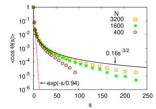 (b)
(b)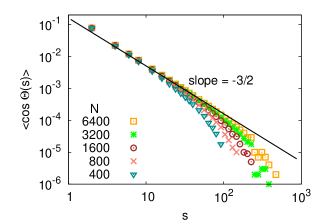
(a)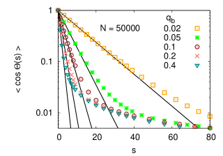 (b)
(b)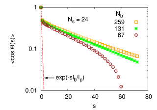
Since the intrinsic stiffness of a chain is a local property of a macromolecule, one might alternatively try the recipe to either fit Eq. (1) in the regime of small to the data, or assume that Eq. (1) holds for already and hence
| (4) |
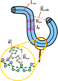
This recipe works in simple cases, such as the SAW model where an energy associated with bond bending is added (every kink of the walk by 90o on the sc lattice costs ), see Fig. 2, but it fails for molecules with more complex chemical architecture, such as bottle-brush molecules 13 ; 14 ; 15 ; 16 . The dramatic failure of Eq. (4) for bottle-brush polymers is understood in terms of their multiscale structure (Fig. 3): The side chains lead to a stiffness of the backbone on a mesoscopic scale, even if on the local scale of nearest-neighbor bonds the backbone is still rather flexible. The question of understanding this stiffening of bottle-brush polymers because of their grafted linear side chains 11 ; 13 ; 14 ; 15 ; 16 ; 17 ; 18 ; 19 ; 20 ; 21 ; 22 ; 23 ; 24 ; 25 ; 26 ; 27 ; 28 ; 29 ; 30 ; 31 ; 32 ; 33 ; 34 ; 35 ; 36 ; 37 ; 38 or grafted branched objects 39 ; 40 ; 41 ; 42 is an issue of longstanding debate in the literature.
Complex polymer architecture is only one out of many reasons which make the analysis of bond orientational correlations based on Eqs. (1) or (4) problematic. In dilute solutions we expect that a nontrivial crossover occurs when the solvent quality is marginal, i.e. close to the Theta point a large size of “thermal blobs” 43 exists, such that for values of along the backbone of the chain corresponding to distances one expects that excluded volume effects are visible and hence Eq. (2) should hold. For semidilute solutions 43 , on the other hand, in the good solvent regime the inverse effect occurs: there exists a screening length depending on the polymer concentration (also called size of “concentration blobs” 43 ), such that excluded volume effects are pronounced for but are absent for . Then Eq. (3) holds for the latter case and Eq. (2) for the former, for rather flexible chains. If the chains are semiflexible, in favorable cases (e.g., for simple chemical architecture of the polymers) we might observe Eq. (1) for where depends on the local intrinsic stiffness of the chain, which we wish to characterize by . Then the question arises whether is smaller than any of the other crossover chemical distances (due to marginal solvent quality, described by a Flory-Huggins parameter with 43 ; 44 , or due to nonzero c) or not. The conclusion of this discussion is that the behavior of bond orientational correlations is subtle, and not always suitable to obtain straightforwardly information on the intrinsic stiffness of macromolecules; as a further caveat we mention that in general it is also not true that this correlation depends on the relative distance only: it matters also, if one of the sites is close to a chain end.
Another popular definition is the local persistence length defined as 1 ; 2
| (5) |
However, it has been shown by renormalization group methods that in good solvents one has, for , , , so the behavior of in the chain interior clearly is unsuitable to conclude anything about the local stiffness of a chain under good solvent conditions, and this conclusion has been corroborated by simulations 11 ; 17 . Sometimes it has been argued that a better choice is to take the correlation between the first bond vector and the end-to-end distance, 46 . However, since in a macromolecule the chemical nature of the end monomer always differs from inner monomers, one can never expect that precisely characterizes the local stiffness of a linear macromolecule in the inner parts of a chain. Moreover, since reflects all the crossovers (due to “thermal blobs” etc.), 43 , as discussed above, it is premature to expect that stays unaffected from them. We also note that for dimensions under good solvent conditions it has been shown 46a that as , so in this case clearly is not a useful measure of the intrinsic stiffness of a chain at all. Since Eq. (5) is difficult to extract from any experiments, and inconvenient for simulation studies due to high sampling effort, we shall not discuss Eq. (5) further in the present paper.
Experimental studies try to extract the persistence length either from scattering analyses of the single chain structure factor (e.g. 28 ; 32 ; 34 ; 35 ; 36 ; 37 ; 38 ; 46b ) or from analyses of extension versus force measurements of stretched chains (e.g. 47 ; 48 ; 49 ; 50 ; 51 ; 52 ; 53 ; 54 ; 55 ). However, the interpretation of the latter experiments must rely on a theoretical model of the extension versus force curve. While this task is simple for ideal random walk models of polymers 4 ; 5 ; 56 and also for semiflexible polymers when excluded volume is neglected 57 , so that the Kratky-Porod (K-P) model 58 of worm-like chains can be used, it is very difficult (due to multiple crossovers 59 ; 60 ) if excluded volume effects are included. These excluded volume effects cause an intermediate nonlinear variation of the extension versus force curve (the chain is then a string of “Pincus blobs” 61 ), making the estimation of the persistence length difficult 60 , and this behavior has also been verified in recent experiments 54 ; 55 . Since we have given a recent extensive discussion of this problem elsewhere 60 , we shall not dwell on this problem here further, and focus on the problem how the persistence length shows up in the single chain structure factor . Here the key idea is that the scattering intensity at scattering wavenumber yields information on the structure of the macromolecule at a length scale . This problem also is subtle, even in the framework of simple models (see Fig. 4a,b,c,d) used for simulations. If is of the scale of the cross sectional radius for the models (a,b,d) or the lattice spacing in (c), local structure on the scale of effective subunits is revealed: soft (a) versus hard (b) effective cylinders, hard spheres in (d), but one could also conceive a chain where soft spheres are jointed, etc. When one considers semiflexible chains with no excluded volume, the persistence length would be just one half of the step length in cases (b), (d), where one then requires a strong bond angle potential to make these chains semiflexible rather than flexible; however, as emphasized above, such models neglecting excluded volume completely will inevitably imply Eq. (1), which is inappropriate for real polymers under all physically possible conditions. So the information on chain stiffness, as described by the persistence length, is hidden in some intermediate range of wavenumbers. E.g., for the model (c), which will be used extensively in the rest of the paper (but in dimensions, since the case of is rather special 60 as will be discussed below), we need wavenumbers in the range , where is the lattice spacing. The aim of the present paper is to present a discussion of how one can obtain detailed information on intrinsic chain stiffness from the gyration radius of the macromolecules and from the structure factor in the suitable intermediate range of wavenumbers .
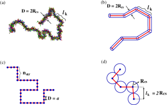
The outline of our paper is as follows: in the next section, we summarize some pertinent theoretical results on . In the third section, our Monte Carlo simulation methods are briefly described. In the fourth section, a comparative discussion of simulation results for two models is given, the bond fluctuation model of bottle-brushes (c.f. Fig. 4a), and the self-avoiding walk model on the simple cubic lattice with variable bending energy (cf. Fig. 4c). The final section contains our conclusions.
II SOME THEORETICAL RESULTS ON THE STRUCTURE FACTOR OF ISOLATED MACROMOLECULES IN SOLUTION
We consider here a single macromolecule with linear chain architecture, assuming a sequence of (effective) monomeric units at positions , , with effective bond vectors , . We have in mind application to standard polymers like polystyrene (disregarding here the scattering from the side groups that are attached to the backbone of the chain, see e.g. Rawiso et al. 46b for a discussion of this problem in an experimental context). We also have in mind application to the scattering from the backbone of bottle-brush polymers (this is experimentally directly accessible from neutron scattering 28 if selective deuteration only of the backbone is used, while in the case of deuteration of the whole macromolecules 32 ; 34 this information can be inferred only indirectly). Due to the restriction to “effective monomeric units” rather than talking about the scattering from individual atoms with the appropriate scattering lengths, we clearly disregard information on the scale of the length of an effective bond, but we then need not discuss experimental problems such as contrast factors between the scattering from the macromolecule and the solvent 46b . The effect of the cross-sectional structure of the chain (finite chain thickness ) is not explicitly considered as well (experimentally this problem often is approximated in terms of the Guinier 71 approximation, writing the observed scattering intensity , with some “effective” cross-sectional radius of the chain 46b . Thus only wavenumbers are physically meaningful: in the case of the lattice model, Fig. 4c, , of course. The structure factor then is defined as
| (6) |
and does not depend on the direction of the scattering wavevector . In dimensions, it has the small expansion
| (7) |
where the mean square gyration radius enters
| (8) |
Other characteristic lengths of the chain molecule are the mean square end-to-end distance
| (9) |
and the contour length
| (10) |
but neither of these lengths can be inferred directly from the scattering. For chains in dense melts or in dilute solutions under Theta conditions one typically uses an ideal chain approximation (disregarding, e.g., logarithmic corrections at the Theta point 3 ; 43 ; 62 )
| (11) |
with a characteristic constant 1 ; 2 ; 3 ; 4 ; 5 . In this case one introduces an equivalent freely jointed Kuhn chain with the same contour length, , where is the number of equivalent Kuhn segments and their length,
| (12) |
For a semiflexible worm-like chain with Eq. (1) holds. However, since under Theta conditions (and melts) Eq. (12) is approximately true, one finds
| (13) |
if the relation then simply is taken as an alternative definition of a persistence length. For the simple SAW model of Fig. 1 this gives lattice spacings: but as expected, using this value in the simple exponential one does not obtain a description of the actual data in Fig. 1 on the basis of this description, because the actual behavior of bond orientational correlations is a power law decay, Eq. (3). Note, however, that the relation makes only sense for semiflexible chains for which at the Theta point, which is not the case for the model of Fig. 1.
In the case of good solvent conditions excluded volume interactions invalidate Eq. (11) and one finds instead 3 ; 7 ; 43 ; 62
| (14) |
with 7 instead of the mean field value that appears in Eq. (13). Note that we have defined the prefactors of the relations , in Eq. (14) in complete analogy with Eq. (13) 11 , but we shall see shortly that the lengths , do not play the role of a persistence length that describes the local intrinsic stiffness of the chains.
For a better understanding of this problem, in particular when is very large, it is of interest to consider the crossover from the rod limit (that occurs for , i.e. ) to the Gaussian coil limit. This problem can be worked out easily for various models of discrete chains 1 ; 2 ; 3 ; 4 ; 5 as well as for the Kratky-Porod model. Describing the chain by a continuous curve , being the curvilinear coordinate along the chain contour, the potential energy of a particular conformation of the chain is given by
| (15) |
In Eq. (15) it is clearly assumed that is a constant, independent of the contour length (or chain length , respectively), and the same holds for . The physical interpretation of is in terms of the local bending stiffness of the chain. Formula (15) can be used for arbitrary values of the ratio , and one can show 58 ; 63
| (16) |
and
| (17) |
One immediately recognizes that for one recovers Eq. (13), while in the opposite limit the results for rigid rods of length are obtained,
| (18) |
However, the generalization of these results to the good solvent case, where excluded volume matters, is not straightforward. Of course, for excluded volume is irrelevant, Eq. (18) remains valid. It turns out, however, that in Eqs. (16), (17) are not valid at all, one has no regime of Gaussian chain behavior as described in Eq. (13), and rather near a crossover from rigid rod behavior to the behavior of two-dimensional self-avoiding walks occurs 60 ; 64 ()
| (19) |
For , however, Eqs. (16), (17) for semiflexible chains remain valid for where . This crossover contour length has first been estimated by a Flory argument as 60 ; 65 ; 66
| (20) |
Note, however, that Flory arguments imply in (rather than the precise value 7 ) and cannot predict any prefactors in Eq. (20); they are based on a crude balancing of the elastic energy of chain stretching (taken as Gaussian) and a mean field estimate of binary interactions: having in mind a model description as in Fig. 4b, one takes the second virial coefficient proportional to the rod volume on the scale of the persistence length, , and in this way the effective chain diameter enters the estimated Eq. (20) 60 ; 65 ; 66 . Numerical results, however, seem to suggest that rather 60 with an exponent
In any case, the conclusion of this discussion is that for semiflexible chains in the mean square radii as a function of the reduced contour length exhibit two successive crossovers, from rods to Gaussian coils near and from Gaussian coils to swollen chains (described by Eq. (14)) near . These two crossovers have in fact been seen nicely in both experiment 67 and computer simulation of the model of Fig. 4c 60 ; 68 ; 69 .
We now turn to a discussion how these behaviors show up in the scattering function at larger wavenumbers, when Eq. (7) does not hold. In the regime , when the chain behaves like a rigid rod, one can work out the scattering function in the continuum limit as 70
| (21) |
while for a discrete chain of scatterers along a rod of length one has
| (22) | |||||
It is noteworthy to recall that the large -limit of Eq. (21) contains information on the contour length and shows a decay,
| (23) |
In the Gaussian regime, that applies for chain lengths that correspond to in , the structure factor is described by the well-known Debye function,
| (24) |
For small , Eq. (24) reduces to Eq. (7), as it must be, while for large Eq. (24) yields . While for flexible chains at the Theta point Eq. (24) is expected to hold for large , up to of order unity where effects due to the local structure of monomeric units comes into play, the validity of Eq. (24) for semiflexible chains is much more restricted, since then the rod to coil crossover matters also with respect to the intrinsic structure of these polymers, as it is probed by . In oder to discuss this problem, it is useful to cast in the representation of the so-called Kratky plot 71 , is plotted as a function of . For rigid rods, one simply would have a linear increase of with for small , which smoothly crosses over near to a flat plateau (which has the value , cf. Eq. (23)). For chains where intermonomer distances follow Gaussian distributions, at all scales, the Kratky plot exhibits a maximum at , and then a crossover to a decay proportional to occurs. To locate this maximum, it is convenient to write as as a function of , noting that the maximum occurs at , i.e. the Kratky plot has its maximum at , and the height of this maximum also is of order . Using now Eq. (13) in the form , we recognize that the maximum of the Kratky plot occurs at
| (25) |
and also the height of this maximum scales proportional to . However, while for flexible chains under Theta conditions (for which and are of the same order), one observes on the Kratky plot for a decay , for semiflexible chains a crossover from this decay to the plateau value (given by Eq. (23)) is expected. This is also true for semiflexible chains under good solvent conditions, if the persistence length is large enough so that , and hence excluded volume effects still can be ignored. The description of this decay of the structure factor from its peak towards this so-called “Holtzer plateau” 72 has been a longstanding problem in the literature 73 ; 74 ; 75 ; 76 ; 77 ; 78 ; 79 ; 80 ; 81 ; 82 ; 83 ; 84 ; 85 ; 86 ; 87 ; 88 ; 89 ; 90 ; 91 ; 92 ; 93 ; 94 . Only in the limit a simple explicit result derived from Eq. (15) is available 78 ,
| (26) |
but we should keep in mind that the limit is well-defined for a simple mathematical continuum model such as Eq. (15), while for real chains (and for simulations) the regime is not at all meaningful. Although the decay , that Eq. (26) predicts for , is compatible with the power law decay of the Debye function, Eq. (24), for large ,
| (27) |
the prefactor in Eq. (27) is by a factor of larger than the prefactor of the term in Eq. (26), so both Eqs. (24) and (26) are inconsistent with each other. This inconsistency is due to the fact that Eq. (26) is only accurate for , it should not be used for small . After many less successful attempts, Kholodenko 84 ; 85 ; 86 ; 87 achieved a description which interpolates between the limiting cases of rigid rods and of Gaussian coils, capturing the scattering law of both limits exactly, but deviating from the exact result (“exact” refers to the Hamiltonian Eq. (15), so no excluded volume effects are being accounted for) in the intermediate regime; this exact behavior is known from systematic expansions 92 ; 93 ; 94 whose use requires heavy numerical work, and will not be considered here. Recently we have shown 95 that the exact method of Stepanow 93 ; 94 deviates only very little from the approximation of Kholodenko 87 , which can be cast in the form
| (28) |
where
| (29) |
with
| (30) |
We stress that all these analytical results Eqs. (11)-(13), (16), (17), (24)-(30) are only applicable if excluded volume effects are negligible. When we consider very long semiflexible chains, such that , we expect that the Gaussian results and hold roughly up to , and there a smooth crossover to the excluded volume power laws, Eq. (14), occurs. We first note that hence corresponds to a crossover radius of the chains as well, . Omitting factors of order unity, we conclude
| (31) |
where in the last step Eq. (20) was used. For we hence expect, invoking the fact that the crossover in the linear dimensions for should be smooth,
| (32) | |||||
where in the last step the Flory estimate was used (recall that in Eq. (31) the exponent defined above has also been put to its Flory value, . In terms of and , Eq. (32) becomes . In terms of the constant defined in Eq. (14), we would have .
The consequences for the scattering function are now clear, since the gyration radius shows the same scaling behavior as , apart from prefactors of order unity. Hence we have
| (33) |
and only for we can expect to see the nontrivial power law
| (34) |
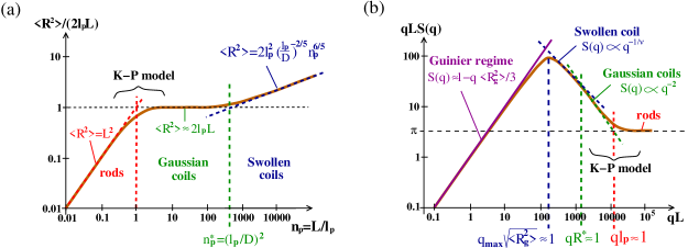
while at defined from we have a smooth crossover to the standard Debye law, . Near then a smooth crossover to the rod-like scattering law occurs. So the three power laws for the radii as a function of chain length in the rod regime, in the regime of Gaussian coils, and in the regime of swollen coils) find their counterpart in the scattering function, if is large enough. The schematic Fig. 5 illustrates these crossover behaviors. The three regimes of the versus (or , respectively) curve, namely rods, Gaussian coils, and swollen coils (Fig. 5a) appear in the vs. curve (or vs. -curve, in the Kratky representation) in inverse order: the rods occur for large , then occurs a first crossover to Gaussian coils, and a second crossover to swollen coils. Of course, if the chains are very stiff but not extremely long, it may be that the regime is not reached: then in part (a) the swollen coil regime is absent, and in part (b) as well: then the K-P model can describe fully, including the regime of the maximum of the Kratky plot. Since the crossovers are smooth, it may be difficult to identify the different power laws in Fig. 5b in practice, however.
We also note that the different regimes are also only well separated if both is very large (in comparison to ) and also needs to be very large. If is very large, but also (as in the case of bottle-brush polymers 11 ; 17 ; 68 ; 69 ) then the regime of Gaussian coils disappears from both Fig. 5a and 5b, and the K-P model loses its applicability.
III MONTE CARLO SIMULATION METHODS AND MODELS
In the present work, we focus on lattice models exclusively, because for them particularly efficient simulation methods exist; pertinent work on coarse-grained off lattice models of bottle-brush polymers studied in Molecular Dynamics methods for variable solvent quality 96 will be mentioned in the conclusions section.
The archetypical lattice model of a polymer is the self-avoiding walk on the simple cubic lattice 97 . Each effective monomer takes a single lattice site, the length of an effective bond is the lattice spacing, so adjacent monomers along the chain are nearest neighbors on the lattice. Double occupancy of lattice sites being forbidden, excluded volume interactions under very good solvent conditions are modelled.
The properties of this basic model are very well established 98 . Solvent quality can be included as a variable into this model implicitly, by allowing for an (attractive) energy that is won if two monomers (that are not nearest neighbors along the chemical sequence of the chain) are nearest neighbors on the lattice. One then finds that the Theta point, at which (apart from logarithmic corrections 3 ; 62 ) the mean square radius scales like a Gaussian chain, , occurs for 12 . On the other hand, if one introduces an energy cost whenever the walk makes a turn by (of course, reversals by 180o are forbidden, because of the excluded volume constraint), one can vary the local intrinsic stiffness of the chain (cf. Fig. 4c, which illustrates this model for dimensions). For one recovers the standard SAW, while the limit corresponds to rigid straight rods. Following up on our previous work 11 ; 60 ; 68 ; 69 ; 95 , we shall focus on this model in the present paper, applying the pruned-enriched Rosenbluth method (PERM) 12 ; 99 . PERM is a biased chain growth algorithm with resampling and allows to get accurate data up to for this model 68 ; 69 . PERM yields a direct estimate of the partition function of a self-avoiding walk with steps and -bends
| (35) |
where is the number of configurations of SAW’s with bonds and a number of turns. It would be interesting to extend the approach from athermal semiflexible chains to semiflexible chains in solvents of variable quality , which would mean an estimation of
| (36) |
with the number of nonbonded nearest neighbor pairs of monomers in the considered configuration. However, we are not aware of any study of the full problem, Eq. (36), yet.
Sampling suitable data on the monomer coordinates of the configurations that contribute to the partition function Eq. (35), one can obtain reasonably accurate estimates of the radii and of , as defined in Sec. 2.
The second model that is studied here is the bond fluctuation model of bottle-brush polymers. In the bond fluctuation model 100 ; 101 ; 102 , each effective monomer blocks all eight corners of the elementary cube of the simple cubic lattice from further occupancy. Two successive monomers along a chain are connected by a bond vector , chosen from the set , , , , , , including also all permutations. Originally configurations were relaxed by an algorithm where a monomer of the chain is chosen at random, and one also randomly chooses one of the six directions (, , or ), respectively, and attempts to move the monomers by one lattice unit in the chosen direction. Of course, the move is accepted only if it does not violate excluded volume or bond length constraints. This move is called the “L6” move. Recently Wittmer et al. 9 provided evidence that a much faster algorithm results if one allows monomers to move to one of the 26 nearest and next nearest neighbor sites surrounding a monomer. With this “L26” move bonds can cross one another, and while such moves do not correspond to a real dynamics of macromolecules, it leads to a much faster exploration of phase space and hence a faster equilibration 103 .
This model for linear polymers is generalized to the bottle-brush architecture by adding side chains at regular spacings (which must be integer, e.g. for a side chain is attached to every second monomer of the backbone; the densest packing that is studied here is . The side chains have chain length , and are described by the bond fluctuation model as well. Furthermore, one more monomer is added to each chain end, to clearly identify the latter. The number of monomers that constitute the backbone then is related to the number of side chains via and the total number of monomers of the bottle-brush polymer is . For the sake of computational efficiency, the L26 move is combined with Pivot moves 98 . We refer to 17 ; 103 for implementation details.
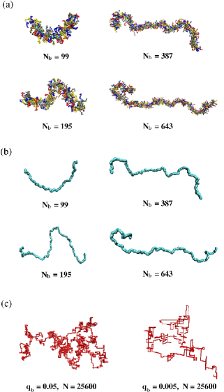
As an example for well-equilibrated bottle-brush polymers as studied in 11 ; 17 ; 68 ; 69 and in the present paper, Fig. 6a shows selected snapshot pictures for side chain length and various backbone chain lengths . According to the visual impression, it seems rather natural to describe these bottle-brush polymers by the worm-like chain model, but as we shall see below, this conclusion would be totally misleading. Experimentalists often are led to a similar conclusion from microscope images of semiflexible polymers (e.g. DNA) adsorbed at a substrate (see e.g. 104 ; 105 ; 106 ). However, such a conclusion is misleading for several reasons: (i) depending on the speed of adsorption of the polymer on the substrate, the conformation of the adsorbed polymer may be a frozen “projection” of the three-dimensional coil, which did not have enough time to relax to the two-dimensional equilibrium. (ii) In dimensions, excluded volume forces render the Kratky-Porod (K-P) model of worm-like chains inapplicable 60 ; 64 , one encounters a direct crossover from the rod regime to two-dimensional self-avoiding walk behavior (cf. Eq. (19)) when the contour length exceeds the persistence length . One also should note that the persistence length of a polymer in dimensions is not at all identical to the persistence length of the same polymer in dimensions 60 ; 64 . The experimental work (see, e.g., 104 ; 105 ; 106 ) seems to be unaware of these problems and the resulting conclusions from this work need to be considered with care. It is also interesting to note that the snapshot pictures of the semiflexible SAW model (Fig. 6c) do not yield an immediate visual impression that the chains can be described by the K-P model, because of the 90o kinks; however, as we shall see, despite this difference of the local structure the statistical properties on the mesoscopic length scales are well described by the K-P model, for and less than . Thus, we argue that on the basis of the inspection of AFM images of semiflexible polymers one should be very careful on drawing conclusions which model is appropriate to describe these polymers.
(a)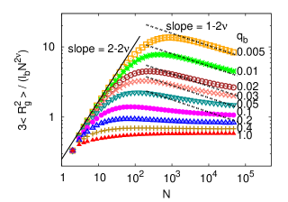 (b)
(b)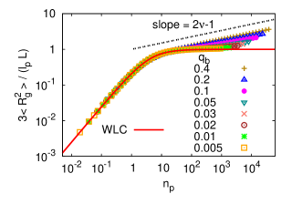
(c)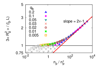
IV SIMULATION RESULTS
IV.1 Mean square gyration radii and their analysis
We start with a description of our results for the mean square gyration radius of the semiflexible SAW model (similar data for the mean square end-to-end distance of this model have already been presented elsewhere 68 ; 69 ), Fig. 7. We clearly see that there are three regimes (Fig. 7a): in the chosen normalization where we divide out the asymptotic power law , we first have a regime where increases with . For small this is interpreted as a rod-like regime; for the chains are still too flexible, however, so a strictly rod-like behavior cannot yet be seen. Then a maximum occurs, and the ratio decreases, before it settles down, after a second smooth crossover at a horizontal plateau (which according to Eq. (14) defines the value ). While this plateau for is (presumably) actually reached for , the data also indicate that for even chains of length =50000 are at least an order of magnitude too short to allow a direct convincing estimation of the amplitude value . On the other hand, even for (where we estimate from Eq. (4) that the persistence length is as large as 60 ) the slope of the data in the intermediate regime has not fully reached the theoretical value , the slope of the data in Fig. 7a is still affected by crossover effects: the gradual crossover away from the Gaussian plateau towards the excluded volume-dominated behavior already starts when the gradual crossover from the rod-like regime to the Gaussian regime ends. Thus, even stiffer chains would be required to have a fully developed Gaussian behavior of the gyration radius. Fig. 7b now attempts a scaling plot, where the persistence length estimates extracted from Eq. (4) were used to rescale in the K-P model representation (cf. Eq. (17)). It is evident that the rod-like regime and the onset of the crossover towards the K-P plateau are very well described by Eq. (17). For , of course, there is basically a direct crossover from the rod-like regime to the excluded volume dominated regime, but even then it is evident that the curves do not superimpose on a master curve, as they do in dimensions 60 ; 64 , but rather splay out systematically, and the smaller becomes (and hence the larger becomes) the more the data still are slightly above the K-P plateau.
Using the estimates for extracted from the analysis of for this model in our previous work 68 ; 69 , the data for do collapse on a simple straight line on the log-log plot, however (Fig. 7c). For near the curves splay out, the master curve describing this second crossover from the K-P plateau to the excluded volume power law emerges as an envelope of the curves for individual values of (which fall increasingly below the master curve in the crossover region the larger is). Of course, cannot produce a scaling of the crossover towards the rod-behavior, there the curves must splay out, irrespective of how small is, but the deviation of the data from the horizontal K-P plateau moves more and more to the left of the plot the smaller becomes.
(a)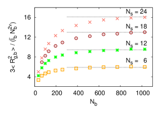 (b)
(b)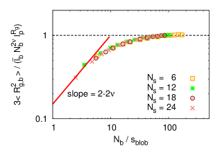
(a)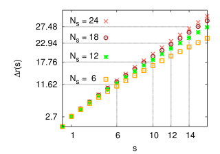 (b)
(b)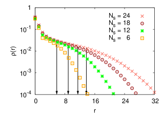
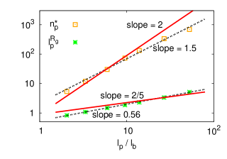
Recalling that for the semiflexible SAW model the effective chain thickness simply is , the Flory theory, Eq. (20), simply predicts ; , while the rod to Gaussian coil behavior occurs around , of course. Qualitatively, our data are in good agreement with these predictions, but not quantitatively: This is illustrated in Fig. 8, where and are plotted in log-log form versus . It is seen that instead of the theoretical value an exponent is observed. Now it is clear that Flory arguments imply also instead of 7 , but this small difference cannot account for the large discrepancy encountered here. It would be desirable to study much larger values of to confirm whether this discrepancy is a real effect (or our estimation of the crossover master curves in Fig. 7c for (and for in 69 ) are systematically off). Thus, more work is still needed to fully clarify the situation.
It turns out that the behavior of our model for the bottle-brush polymers (which can describe actual scattering data for bottle-brush polymers very well, as demonstrated by Hsu et al. 17 ) is much simpler: a plot of the mean square gyration radius of the backbone versus backbone chain length , for different side chain lengths , Fig. 9a, normalized by reveals a monotonic increase towards a plateau, there is not the slightest indication of a regime where the ratio decreases, unlike the behavior of the semiflexible SAW (Fig. 7a). Thus, there is no evidence whatsoever for a Gaussian K-P plateau for this model. But the increase of the plateau value with increasing side chain length does indicate that the chain considerably stiffens, as increases. However, this stiffening goes along with an increase in the effective chain thickness . The latter can be estimated from the radial density profile (Fig. 10) by identifying the diameter of the bottle-brush as . Hsu et al. 68 ; 69 suggested to coarse-grain the bottle-brush along the backbone, dividing it into “blobs” along the chemical sequence of the backbone. The chemical distance along the backbone between its exit and entry points into a blob is found from a simple construction which assumes that the blobs are essentially spherical, so the geometrical distance between exit and entry points of the backbone should be equal to . Recording for arbitrary , Fig. 10a, using the equation allows us to simply read off the numbers for the choices of , as illustrated in Fig. 10. The success of the rescaling shown in Fig. 9b shows that the persistence length of bottle-brushes simply is proportional to . We also recognize that the asymptotic SAW-like behavior (where the horizontal plateau in Fig. 9 is reached) only occurs for about Comparing this behavior to Fig. 7b, we see that there the power law (for ) or K-P plateau (for small ) is reached for . Roughly, these successive blobs then are equivalent to one persistence length. This comparison suggests that for the bottle-brushes we should identify with , i.e. the number of monomers along the backbone corresponding to one persistence length is , , and for , , and , respectively. Noting that the average bond length in the bond fluctuation model is , we would obtain persistence lengths , , and for , , and , respectively. The result that is of the same order as irrespective of the side chain length agrees with early theoretical predictions 18 ; 19 but is at variance with the result of Fredrickson 20 who predicted a much faster increase of with . However, Feuz et al. 30 pointed out that the result of Fredrickson 20 can only be expected to hold for extremely long side chains, such as . Such long side chains are neither relevant for simulations nor for experiment, however. We stress that the range of accessible to simulations (Figs. 9, 10) nicely corresponds to the range of studied experimentally 28 ; 32 ; 33 ; 34 ; 35 ; 36 ; 37 ; 38 .
The mapping performed in Fig. 9 means that we have coarse-grained the bottle-brush polymers (Fig. 4a) into an effective bead-spring model (Fig. 4d). If this mapping is taken literally, it can also be used to obtain the resulting coarse-grained contour length (Fig. 3) as
| (37) |
Instead of the “chemical” contour length a reduced length is found, namely , , and , for , , and , respectively. This means that the coarse-grained contour length is about smaller than the “chemical” contour length in this model.
(a)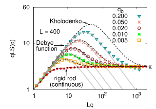 (b)
(b)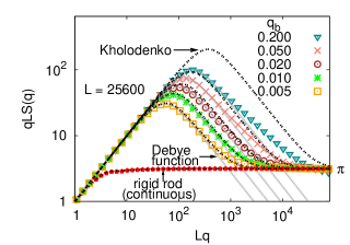
(c)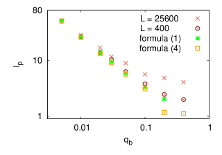
IV.2 Analysis of the structure factor
We now turn to the structure factor of the semiflexible SAW model presenting Kratky plots for two contour lengths, and , in Fig. 11. As expected, cf. Fig. 5, one first has a linear increase with , then a round maximum followed by a decrease which then gradually settles down at a horizontal plateau, that again is compatible with the theoretical prediction, .
While for the short chain length () the agreement with the theoretical prediction (due to Kholodenko 87 , Eqs. (28)-(30), which were found 95 to be numerically almost indistinguishable from the exact result provided by Stepanow 93 ; 94 ) is almost perfect, for the very long chains we note systematic deviations between Kholodenko’s prediction 87 and the data for relatively large near the maximum of the Kratky plot. This must be expected, since the input in the Kholodenko formula is just the persistence length {which we have extracted from Eq. (4)} and implicit in the theory is the Gaussian prediction for , namely {Eq. (13)}. As seen in Fig. 7, for already rather clear deviations from this result occur for , while for small such as such deviations still are rather small. In contrast, in the Debye formula the correct (as observed) value of was used as an input: then deviations from the Debye function are only seen near the region where the crossover to starts to set in at large (the Debye function does not describe this crossover at all). Since the shape of the Kholodenko function always is rather similar to the actual function, it is obvious that one always can fit the data to the Kholodenko function, if is not known: however, the resulting fitted persistence length will be systematically too large, if excluded volume effects are present as shown in Fig. 11c.
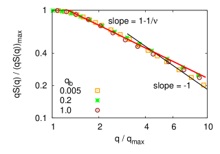
To elucidate the significance of excluded volume on the structure factor further, we show a magnification of the region near the maximum for , , and in Fig. 12. It is seen that the identification of the two power laws suggested for the decay of in the region beyond the maximum of the Kratky plot is rather subtle. In particular, for rather stiff chains the crossover to the rod-like scattering sets in rather early, so for the clear identification of power laws the available range of simply is not large enough. This very gradual crossover between the three different regimes (rods to Gaussian coils to coils swollen by the excluded volume interaction) complicates the data analysis, if only a restricted range of parameters (such as the chain length and the wavenumber ) can be investigated.
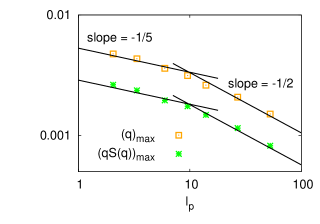
The smoothness of the crossover also becomes evident when one studies the dependence of the position of the peak in the Kratky-plot (and its height) on the persistence length (Fig. 13). Typically, the data fall neither in the regime where strict Gaussian behavior occurs, nor in the regime where excluded volume scaling is fully developed.
Despite all these difficulties due to the gradual crossovers, the semiflexible SAW nevertheless is a relatively simple case, since one knows that here , and can be varied over a wide range by variation of , keeping all other parameters constant, and moreover can be estimated precisely from the initial decay of the bond vector autocorrelation function (or, equivalently, from Eq. (4)). For the second model studied here, bottle-brush polymers under good solvent conditions, we have seen that varying the side chain length we change and together, and also the coarse-grained contour length is significantly smaller than the chemical contour length , and it is nontrivial to estimate accurately.
(a)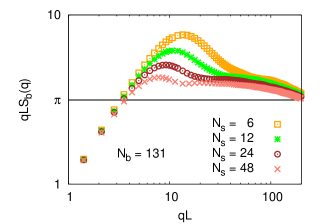 (b)
(b)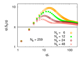
In previous work 11 ; 17 we have already considered the decomposition of the total scattering function of bottle-brush polymers into the scattering from the backbone and from the side chains. This analysis which has the advantage that it provides a direct link to corresponding experiments 32 ; 33 will not be addressed here, but we rather focus on the scattering function of the backbone only. Fig. 14 shows Kratky plots for relatively short backbone chain lengths ( and 259, respectively). One recognizes that for short side chain lengths ( does not settle down to a well-defined “Holtzer Plateau”, at least not within the available window of wavenumbers. Clearly, also the range over which decays from the maximum to the horizontal part that appears for and is rather small, and does not warrant any analysis in terms of the power laws suggested in Fig. 5b. This mismatch between the actual plateau values (for and ), which are close to , and the theoretical value can be attributed to reduction of in comparison to since the actual orientations of the backbone vectors are not strictly aligned with the coarse-grained backbone (Fig. 4), as is also evident from the fact that (Fig. 2b) is already reduced to about , but the further decrease of is rather slow, due to the side chain induced stiffening of the backbone on mesoscopic scales. The ratio at about is compatible with the reduction of by about relative to noted previously, so gratifyingly our analysis is internally consistent.

Fig. 15 shows plots of vs. for fixed side chain length =24 but different backbone chain lengths. In this plot, an attempt is made to locate an onset wavenumber for the Holtzer plateau, in terms of a fit of two intersection straight lines. Of course, the data are smooth and the onset of the Holtzer plateau does not occur sharply but rather gradual; thus can be estimated only with considerable error (for large we estimate , while for the estimate rather is 11 ). Now the question is, how can one relate explicitly to the persistence length? Should one take , or ? Lecommandoux et al. 28 who were the first to try such a method suggested the relation , but we see little theoretical support for this choice either.
It would be advantageous if one could rely on the des Cloizeaux relation, Eq. (26), which suggests to plot vs. for : one should find a straight line, the intercept at the ordinate should yield , the slope of the straight line should yield .
However, when one tests this method for the semiflexible SAW, one finds that the data that can be fitted to a straight line are at rather than at , and the slope of the straight line disagrees with the prediction (Fig. 16a). Thus, it is not really a big surprise that this does not work well for our bottle-brush model either (Fig. 16b).
(a)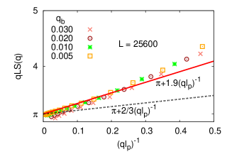 (b)
(b)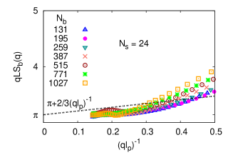
(a)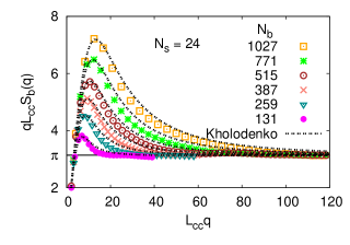 (b)
(b)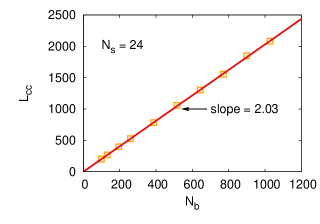
(c)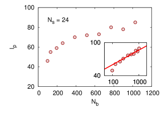
An interesting alternative of data analysis is, however, a fit of the Kholodenko formulas {Eqs. (28)-(30)} to the structure factor, using both and as individual adjustable parameters for each value of (Fig. 17). First of all, one sees that the Kholodenko structure factor provides a good fit in all cases, and the result for the coarse-grained contour length, , even is physically very reasonable: we have obtained that there is a 30% reduction of the in comparison to the “chemical” contour length in the previous subsection.
However, the problem of this fit is the unphysical behavior of the persistence length : since we know that the Kholodenko 87 approach involves necessarily the Gaussian result but we know that for our model and , the only way to reconcile these results is a persistence length scaling as , and this is what we see in Fig. 17c. Thus, despite the seemingly good fit (Fig. 17a) and good results for (Fig. 17b), the results for the persistence lengths are completely unreliable!
In order to apply this approach, one must make sure that one works with data in the Gaussian regime, and this is not at all the case for bottle-brush polymers under good solvent conditions.
V Conclusions
In this paper, we have focused on the behavior of single semiflexible polymers under very good solvent conditions, considering how the chain stiffness affects polymer properties such as the mean square gyration radius, the structure factor, etc. Our analysis focused on the question how the variation of chain stiffness affects these properties, and hence one can infer from these properties a characterization of the “intrinsic stiffness” of the polymer chain in terms of the so-called “persistence length”.
We have contrasted two models, the self-avoiding walk on the simple cubic lattice where a bending energy causes pronounced stiffening of the polymer when , and a lattice model for bottle-brush polymers, where backbone stiffening is caused by increasing the length of side chains. These two models constitute two quite distinct limiting cases: in the SAW model, increase of causes stiffening without any effect on the local thickness of the chain, which strictly remains the lattice spacing. For the bond fluctuation model of polymer brushes, however, we have found that backbone stiffening is caused by the thickness of the (coarse-grained) worm-like chain, the persistence length increases proportional to the cross-sectional diameter of the bottle-brush.
Since snapshot pictures (Fig. 6) suggest that the bottle-brush polymers (or their backbones, respectively) resemble worm-like chains (and the same conclusion is often drawn from AFM pictures or electron micrographs of actual polymers), the use of the Kratky-Porod worm-like chain model has become very popular. However, we demonstrate here that for bottle-brush polymers this model yields very misleading results: since the mean square gyration radii of bottle-brushes are found to scale with their contour length as , the Kratky-Porod (K-P) result invariably causes a spurious contour length dependence of the persistence length when fit to the data, namely as . Although the fits of the K-P model look almost perfect (Fig, 17a) and numbers for resulting for the contour length from the fit are rather reasonable, the result for “the” persistence length simply is meaningless!
Already in our earlier papers we have shown that similar ambiguous results for the persistence length are gotten when orientational correlations along the chain backbone are analyzed, or the projection of bond vectors on the end-to-end distance are studied (although the resulting numbers for seem to be somewhat smaller than those shown in Fig. 17c). The large -behavior of the structure factor yields a qualitatively more reasonable behavior, but a unique choice for a well-defined persistence length as a measure for intrinsic chain stiffness does not emerge. All these difficulties in understanding the stiffness of bottle-brush polymers in good solvents are intimately linked to the fact that one can coarse-grain into some effective self-avoiding walk model (Figs. 9, 10), and no regime exists where the polymers resemble Gaussian chains. Of course, this fact is different if we would consider bottle-brush polymers in Theta-solvents (as done by Theodorakis et al. 96 ), since then and the use of the K-P model is qualitatively reasonable. Another interesting possibility to extract a persistence length of bottle brushes would be an attempt to estimate an effective bending modulues. One would have to estimate the coarse-grained free energy of bent versus non-bent configurations of suitable pieces of bottle-brush polymers, which in principle can be deduced from sampling suitable angular distribution functions for such sub-chains. However, the implementation of such an approach is not straightforward and has not been attempted.
We have found that the situation in some respects is simpler if one considers polymers where the stiffness can be enhanced while keeping their thickness constant, as modeled by a semiflexible extension of the standard SAW model. Then an intermediate Gaussian-like behavior of the mean square radii and the structure factor emerges, and this can be understood theoretically (Fig. 5), at least in qualitative terms. While still the asymptotic decay of bond vector autocorrelation functions is unsuitable to infer anything about the intrinsic stiffness (due to the fact that the asymptotic decay is not exponential but rather described by a power law), in favorable cases the initial decay of these autocorrelation functions provided useful estimates of the persistence length, which then can be used as input in the K-P model. While still some problems occur to understand for very long chain the crossover between the K-P model and the ultimate SAW behavior, quantitatively, in qualitative terms the situation is understood. We emphasize, however, that all these comments only address the three-dimensional case: in dimensions, the K-P model does not work at all, and one has a direct crossover from rod-like polymers to SAW’s.
It is hoped that our analysis will help experimentalists with a proper interpretation of their data on semiflexible polymers.
Acknowledgements.
We are grateful to the Deutsche Forschungsgemeinschaft (DFG) for support under grant No SFB 625/A3, and to the John von Neumann Institute for Computing (NIC Jülich) for a generous grant of computer time. We are particularly indebted to S. Stepanow for his help with the explicit calculation of his exact formula for the structure factor of the Kratky-Porod model. We are also indebted to Hyuk Yu for pointing out Ref. 67 to us. H.-P. Hsu thanks K. Ch. Daoulas for stimulating discussions.References
- (1) P. J. Flory, Statistical Mechanics of Chain Molecules (Interscience, New York, 1969).
- (2) H. Yamakawa, Modern Theory of Polymer Solutions (Harper and Row, New York, 1971).
- (3) J. Des Cloizeaux and G. Jannink, Polymers in Solution: Their Modelling and Structure (Clarendon Press, Oxford, 1990).
- (4) A. Yu. Grosberg and A.R. Khokhlov, Statistical Physics of Macromolecules (AIP Press, New York, 1994).
- (5) M. Rubinstein and R. H. Colby, Polymers Physics (Oxford, 2003).
- (6) L. Schäfer, A. Ostendorf and J. Hager, J. Phys. A: Math. Gen. 32, 7875 (1999).
- (7) J. C. Le Guillou and J. Zinn-Justin, Phys. Rev. B 21, 3976 (1980).
- (8) J. P. Wittmer, H. Meyer, J. Baschnagel, A. Johner, S. Obukhov, L. Mattioni, M. Müller, and A. N. Semenov, Phys. Rev. Lett. 93, 147801 (2004).
- (9) J. P. Wittmer, P. Beckrich, H. Meyer, A. Cavallo, A. Johner, and J. Baschnagel, Phys. Rev. E 76, 011803 (2007).
- (10) D. Shirvanyants, S. Panyukov, Q. Liao, and M. Rubinstein, Macromolecules 41, 1475 (2008).
- (11) H.-P. Hsu, W. Paul, and K. Binder, Macromolecules 43, 3094 (2010).
- (12) P. Grassberger, Phys. Rev. E 56, 3682 (1997).
- (13) M. Zhang and A. H. E. Müller, J. Polym. Sci, Part A: Polym. Chem.: 43, 3461 (2005).
- (14) A. V. Subbotin and A. N. Semenov, Polym. Sci. Ser. A 49, 1328 (2007).
- (15) S. S. Sheiko, B. Sumerlin, and K. Matyjaszewski, Progr. Polym. Sci. 33, 759 (2008).
- (16) I. I. Potemkin and V. V. Palyulin, Polym. Sci. Ser. A 51, 123 (2009).
- (17) H.-P. Hsu, W. Paul, S. Rathgeber, and K. Binder, Macromolecules, 43, 1592 (2010).
- (18) T. M. Birshtein, O. V. Borisov, E. B. Zhulina, A. R. Khokhlov, and T. A. Yurasova, Polym. Sci. USSR 29, 1293 (1987).
- (19) O. V. Borisov, T. M. Birshtein, and E. B. Zhulina, Polym. Sci. USSR 29, 1552 (1987).
- (20) G. H. Fredrickson, Macromolecules 26, 2825 (1993).
- (21) Y. Rouault and O. V. Borisov, Macromolecules 29, 2605 (1996).
- (22) M. Saariaho, O. Ikkala, I. Szleifer, I. Erukhimovich, and G. ten Brinke, J. Chem. Phys. 107, 3267 (1997).
- (23) M. Saariaho, I. Szleifer, O. Ikkala, and G. ten Brinke, Macromol. Theory Simul. 7, 211 (1998).
- (24) Y. Rouault, Macromol. Theory Simul. 7, 359 (1998).
- (25) M. Saariaho, A. Subbotin, I. Szleifer, O. Ikkala, and G. ten Brinke, Macromolecues 32, 4439 (1999).
- (26) K. Shiokawa, K. Itoh, and N. Nemoto, J. Chem. Phys. 111, 8165 (1999).
- (27) A. Subbotin, M. Saariaho, O. Ikkala, and G. ten Brinke, Macromolecules 33, 3447 (2000).
- (28) S. Lecommandoux, F. Chéoct, R. Borsali, M. Schappacher, A. Deffieux, A. Brûlet, and J. P. Cotton, Macromolecules 35, 8878 (2002).
- (29) S. Elli, F. Ganazzoli, E. G. Timoshenko, Y. A. Kuznetsov, R. Connolly, J. Chem. Phys. 120, 6257 (2004).
- (30) L. Feuz, F. A. Leermakers, M. Textor, and O. V. Borisov, Macromolecules 38, 8891 (2005).
- (31) B. Connolly, G. Bellesia, E. G. Timoshenko, Y. A. Kuznetsov, S. Elli, and F. Ganazzolli, Macromolecules 38, 5288 (2005).
- (32) S. Rathgeber, T. Pakula, K. Matyjaszewski, and K. L. Beers, J. Chem. Phys. 122, 124904 (2005).
- (33) A. Yethiraj, J. Chem. Phys. 125, 204901 (2006).
- (34) B. Zhang, F. Gröhn, J. S. Pedersen, K. Fischer, and M. Schmidt, Macromolecules 39, 8440 (2006).
- (35) L. Feuz, P. Strunz, T. Geue, M. Textor, and O. V. Borisov, Eur. Phys. J. E 23, 237 (2007).
- (36) L. A. Bastardo, J. Iruthayaraj, M. Lundin, A. Dedinaite, A. Vareikis, R. Makuka, A. van der Wal, I. Furó, V. M. Garamus and P. M. Claesson, J. Colloid Interface Sci. 312, 21 (2007).
- (37) G. Cheng, Y. B. Melnichenko, G. D. Wignall, F. Hua, K. Hong, and J. W. Mays, Macromolecules 41, 9831 (2008).
- (38) S. Bolisetty, S. Rosenfeldt, C. N. Rochette, L. Harnau, P. Lindner, Y. Xu, A. H. E. Müller, and M. Ballauff, Colloid Polym. Sci 287, 129 (2009).
- (39) A. D. Schlüter and J. P. Rabe, Angew. Chem., Int. Ed. 39, 864 (2000).
- (40) D. Yan, C. Gao, and H. Frey (Eds.) Hyperbranched Polymers: Synthesis, Properties, and Applications (Wiley-VCH, Weinheim, 2011).
- (41) O. V. Borisov, E. B. Zhulina, and T. M. Birshtein, ACS Macro Letters (2012, in press).
- (42) H. Rabbel, Diplomarbeit (Johannes Gutenberg Universität Mainz, 2012, unpublished).
- (43) P. G. de Gennes, Scaling Concepts in Polymer Physics (Cornell Univ. Press, Ithaca, N.Y., 1979).
- (44) P. J. Flory, Principles of Polymer Chemisty (Cornell Univ. Press, Ithaca, N.Y., 1953).
- (45) L. Schäfer and K. Elsner, Eur. Phys. J. E 13, 225 (2004).
- (46) P. Cifra, Polymer 45, 5995 (2004).
- (47) S. Redner and V. P. Privman, J. Phys. A: Math. Gen. 20, L857 (1987).
- (48) M. Rawiso, R. Duplessix, and C. Picot, Macromolecules 20, 630 (1987).
- (49) S. B. Smith, L. Finzi, and C. Bustamante, Science 258, 1112 (1992).
- (50) M. Rief, M. Gautel, F. Oesterhelt, J. M. Fernandez, and H. E. Gaub, Science 276, 1109 (1997).
- (51) M. Grandbois, M. Beyer, M. Rief, H. Clausen-Schaumann and H. E. Gaub, Science 283, 1727 (1999).
- (52) J. Liphardt, B. Onoa, S. B. Smith, I. Tinoco Jr., and C. Bustamante, Science 292, 733 (2001).
- (53) M.-N. Dessinges, B. Maier, Y. Zhang, M. Peliti, D. Bensimon, and V. Croquette, Phys. Rev. Lett. 89, 248102 (2002).
- (54) Y. Seol, G. M. Skinner, and K. Visscher, Phys. Rev. Lett. 93, 118102 (2004).
- (55) N. Gunari, M. Schmidt, and A. Janshoff, Macromolecules 39, 2219 (2006).
- (56) O. A. Saleh, D. B. McIntosh, P. Pincus, and N. Ribeck, Phys. Rev. Lett. 102, 068301 (2009).
- (57) A. Dittmore, D. B. McIntosh, S. Halliday, and O. A. Saleh, Phys. Rev. Lett. 107, 148301 (2011).
- (58) M. Fixman and J. Kovac, J. Chem. Phys. 58, 1564 (1973).
- (59) J. F. Marko and E. D. Siggia, Macromolecues 28, 8759 (1995).
- (60) O. Kratky and G. Porod, J. Colloid Sci. 4, 35 (1949).
- (61) N. M. Toan and D. Thirumalai, Macromolecules 43, 4394 (2010).
- (62) H.-P. Hsu, and K. Binder, J. Chem. Phys. 136, 024901 (2012).
- (63) P. Pincus, Macromolecules 9, 386 (1976).
- (64) L. Schäfer, Excluded Volume Effects in Polymer Solutions: as Explained by the Renormalization Group, Springer, Berlin 1999.
- (65) H. Benoit and P. Doty, J. Phys. Chem. 57, 958 (1953).
- (66) H.-P. Hsu, W. Paul, and K. Binder, EPL 95, 68004 (2011).
- (67) D. W. Schaefer, J. F. Joanny, and P. Pincus, Marcomolecules 13, 1280 (1980).
- (68) R. R. Netz and D. Andelman, Phys. Rep. 380, 1 (2003).
- (69) T. Norisuye and H. Fujita, Polymer J.14, 143 (1982).
- (70) H.-P. Hsu, W. Paul, and K. Binder, EPL 92, 28003 (2010).
- (71) H.-P. Hsu, W. Paul, and K. Binder, Macromol. Theory Simul. 20, 510 (2011).
- (72) T. Neugebauer, Ann. Phys. 434, 509 (1943).
- (73) J. S. Higgins and H. C. Benoit, Polymers and Neutron Scattering (Clarendon Press, Oxford, 1994).
- (74) A. Holtzer, J. Polym. Sci. 17, 432 (1955).
- (75) G. Porod, J. Polym. Sci. 10, 157 (1953).
- (76) J. Hermans and J. J. Hermans, J. Phys. Chem. 62, 1543 (1958).
- (77) A. Peterlin, J. Polym. Sci. 47, 403 (1960).
- (78) H. Yamakawa and. W. H. Stockmayer, J. Chem. Phys. 57, 2843 (1972).
- (79) R. Koyama, J. Phys. Soc. Japan 34, 1029 (1973).
- (80) J. des Cloizeaux, Macromolecules 6, 403 (1973).
- (81) W. R. Krigbaum and S. Sasaki, J. Polym. Sci.: Polym. Phys. Ed. 19, 1339 (1981).
- (82) H. Yamakawa and J. Shimada, J. Chem. Phys. 83 2607 (1985).
- (83) M. G. Bawendi and K. F. Freed, J. Chem. Phys. 83, 2491 (1985).
- (84) J. Shimada and H. Yamakawa, J. Chem. Phys. 85, 591 (1986).
- (85) H. Fujita, Macromolecules 21, 179 (1988).
- (86) A. L. Kholodenko, Ann. Phys. 202, 186 (1990).
- (87) A. L. Kholodenko, J. Chem. Phys. 96, 700 (1992).
- (88) A. L. Kholodenko, Phys. Lett. A 178, 180 (1993).
- (89) A. L. Kholodenko, Macromolecules 26, 4179 (1993).
- (90) J. S. Pedersen, M. Laso and P. Schurtenberger, Phys. Rev. E 54, R5917 (1996).
- (91) J. S. Pedersen and P. Schurtenberger, Macromolecules 29, 7602 (1996).
- (92) J. S. Pedersen and P. Schurtenberger, Europhys. Lett. 45, 666 (1999).
- (93) D. Pötschke, P. Hickl, M. Ballauff, P.-O. Astrand, and J. S. Pedersen, Macromol. Theory Simul. 9, 345 (2000).
- (94) A. J. Spakowitz and Z.-G. Wang, Macromolecules 37, 5814 (2004).
- (95) S. Stepanow, Eur. Phys. J. B 39, 499 (2004).
- (96) S. Stepanow, J. Phys.: Condens. Matter 17, S1799 (2005).
- (97) H.-P. Hsu, W. Paul, and K. Binder, J. Chem. Phys. 137, 174902 (2912).
- (98) P. E. Theodorakis, H.-P. Hsu, W. Paul, and K. Binder, J. Chem. Phys. 135, 164903 (2011).
- (99) K. Kremer and K. Binder, Computer Phys. Rep. 7, 259 (1988), and references therein.
- (100) A. D. Sokal, in Monte Carlo and Molecular Dynamics Simulations in Polymer Science (K. Binder, ed.) Chap. 2 (Oxford Univ. Press, New York, 1995).
- (101) H.-P. Hsu and P. Grassberger, J. Stat. Phys. 144, 597 (2011).
- (102) I. Carmesin and K. Kremer, Macromolecules 21, 2819 (1988).
- (103) H. P. Deutsch and K. Binder, J. Chem. Phys. 94, 2294 (1991).
- (104) W. Paul, K. Binder, D. W. Heermann and K. Kremer, J. Phys. II (France) 1, 37 (1991).
- (105) H.-P. Hsu and W. Paul, Comp. Phys. Comm. 182, 2115 (2011).
- (106) N. Yoshinaga, K. Yoshikawa and S. Kidoaki, J. Chem. Phys. 116, 9926 (2002).
- (107) J. Moukhtar, E. Fontaine, C. Faivre-Moskalenko, and A. Arneodo, Phys. Rev. Lett. 98, 178101 (2007).
- (108) J. Moukhtar, C. Faivre-Moskalenko, P. Milani, B. Audit, C. Vaillant, E. Fontaine, F. Mongelard, G. Lavorel, P. St.-Jean, P. Bouvet, F. Argoul, and A. Arneodo, J. Phys. Chem. B 114, 5125 (2010).