Shock problem for MKdV equation: Long-time Dynamics of the Step-like Initial Data

Abstract

We consider the modified Korteveg de Vriez equation on the whole line. Initial data is real and step-like, i.e. $q(x,0)=0$ for $x\geq 0$ and $q(x,0)=c$ for $x<0$, where c is arbitrary real number. The goal of this paper is to study the asymptotic behavior of the initial-value problem’s solution by means of the asymptotic behavior of the some Riemann–Hilbert problem. In this paper we show that the solution of this problem has different asymptotic behavior in different regions. In the region $x<-6c^{2}t$ and $x>4c^{2}t$ the solution is tend to $c$ and $0$ correspondingly. In the region $-6c^{2}t<x<4c^{2}t$ the solution takes the form of a modulated elliptic wave.

1 Introduction

Initial value problems with step-like initial function have very long story beginning from the papers by A.V. Gurevich, L.P. Pitaevsky [8] and E.Ya.Khruslov [9] in a middle of 70th. There are many papers devoted to different aspects of these problems. For the present time there are a few full and rigorous results on an asymptotic behavior of such problems [10], [Bik1]-[Bik5], [16],…..,. We pay our attention here to a problem which was not considered elsewhere and give results in a rigorous form using the method of the matrix Riemann-Hilbert problem and the steepest descent method for oscillatory matrix RH problems. We consider the modified Korteweg de Vries equation on the whole line. Initial datum is a step-like, i.e. $q(x,0)=0$ for $x\geq 0$ and $q(x,0)=c$ for $x<0$, where $c$ is an arbitrary real number. Without loss of generality we put $c>0$. This problem can be considered as a shock problem. The goal of this paper is to study asymptotic behavior of the Riemann –Hilbert problem whose solution gives the solution of the initial-value problem. In this paper we show that the solution of the shock problem has different asymptotic behavior in different regions. In the regions $-\infty<x<-6c^{2}t$ and $4c^{2}t<x<\infty$, the solution is trivial, i.e. it is equal to $c$ and $0$ respectively. In the region $-6c^{2}t<x<-4c^{2}t$ the solution takes the form of a modulated elliptic wave of finite amplitude. Thus for a large time the solution has finite amplitude in the first two regions while in the third region ($4c^{2}t<x<\infty$) it takes the form of a vanishing (as $\mathrm{O}(t^{-1/2})$) self-similar wave. The development of the Riemann-Hilbert method for the shock problems arising for integrable PDEs on the whole line with the different finite-gap boundary conditions as $x\to\pm\infty$ goes back to the works done in 80-90s by R. Bikbaev, P. Deift, V. Novokshenov, and S. Venakides. All those results was devoted to the initial-value problem with self-adjoint Lax operators. Most recently, an implementation of the RH scheme to the shock problem and the evaluation of the long-time asymptotics of the solution to the focusing nonlinear Schrödinger equation on the whole line, where the Lax operator is not self-adjoint and the initial function was chosen in the form $q(x,0)=A\exp{(i\mu|x|)}$, was done in [16]. It is worth mentioning that our shock problem is different from that in [16] as well as our construction of the phase $g$ - function.

The inverse scattering transform method (IST) for solving initial-value problems for nonlinear evolutionary equations, discovered in 1967 [1], turned out to be a very powerful tool, which allowed to obtain a huge number of very interesting results in different areas of mathematics and physics. At the beginnig of 90th a new great achievement in the further development of the IST method have been done by P.Deift and X.Zhou. It is a nonlinear steepest descent method for oscillatory matrix Riemann-Hilbert problem. With the new method it came a nice possibility to rewrite known asymptotic results for different nonlinear integrable models in the rigorous and transparent form (sf.[11],[12],[13]) and obtain numerous new significant results in the theory of completely integrable nonlinear equations, random matrix models and orthogonal polynomials, integrable statistical mechanics. Our goal is to bring new results in theory of the shock problems, especially in the case of non self-adjoint Lax operators, and some development of ideas, given recently in [17], [18] in the direction of the strengthening of the nonlinear steepest descent method for oscillatory matrix Riemann-Hilbert problem.

Let us consider the problem

$$q_{t}+6q^{2}q+q_{xxx}=0$$ (1.1)

$$q(x,0)=q_{0}(x)\rightarrow\begin{cases}0,\quad x\rightarrow+\infty\\ c,\quad x\rightarrow-\infty,\end{cases}$$ (1.2)

where $q_{0}(x)$ is arbitrary step-like function, including the discontinuous case: $q_{0}(x)\equiv c$ for $x<0$ and $q_{0}(x)\equiv 0$ for $x\geq 0$. We suppose that the solution $q(x,t)$ of this problem exists for $x\in\mathbb{R},t\in\mathbb{R}_{+}$. To study the initial value problem (1.1)-(1.2) we will use the Lax representation of the MKdV equation in the form of over-determined system of differential equations:

$$\Phi_{x}+ik\sigma_{3}\Phi=Q(x,t)\Phi$$ (1.3)

$$\Phi_{t}+4ik^{3}\sigma_{3}\Phi=\hat{Q}(x,t,k)\Phi,$$ (1.4)

where $\Phi=\Phi(x,t,k)$ is a $2\times 2$ matrix-valued function,

$$\sigma_{3}:=\begin{pmatrix}1&0\\ 0&-1\end{pmatrix},\qquad Q(x,t):=\begin{pmatrix}0&q(x,t)\\ -q(x,t)&0\end{pmatrix},$$ (1.5)

$$\hat{Q}(x,t,k)=4k^{2}Q(x,t,k)-2ik(Q^{2}(x,t,k)+Q_{x}(x,t,k))\sigma_{3}+2Q^{3}(x,t,k)-Q_{xx}(x,t,k),$$ (1.6)

and $k\in\mathbb{C}$. The equations (1.3) and (1.4) are compatible if and only if the function $q(x,t)$ satisfy the MKdV equation (1.1). To apply the inverse scattering transform to the problem (1.1), (1.2) we have to construct matrix valued solution of this equations defined by their asymptotics:

$$\Phi(x,t,k)=e^{-(ikx+4ik^{3}t)\sigma_{3}}+\mathrm{O}\left(\frac{1}{k}\right),\quad x\to+\infty,\quad\operatorname{Im}k=0$$ (1.7)

$$\Psi(x,t,k)=E(x,t,k)+{\mathrm{O}}\left(\frac{1}{k}\right),\quad x\rightarrow-\infty,\quad\operatorname{Im}k=0.$$ (1.8)

Here $E(x,t,k)$ is the solution of the linear differential equations

$$\\ E_{x}+ik\sigma_{3}E=Q_{c}E$$ (1.9)

$$E_{t}+4ik^{3}\sigma_{3}E=\hat{Q}_{c}(k)E,$$ (1.10)

where

$$Q_{c}:=\begin{pmatrix}0&c\\ -c&0\end{pmatrix}$$ (1.11)

$$\hat{Q}_{c}(k)=4k^{2}Q_{c}-2ikQ_{c}^{2}\sigma_{3}+2Q_{c}^{3}.$$ (1.12)

We chose the solution $E(x,t,k)$ as follows:

$$E(x,t,k)=\displaystyle\frac{1}{2}\left(\begin{array}[]{ccc}\varkappa(k)+\displaystyle\frac{1}{\varkappa(k)}&\varkappa(k)-\displaystyle\frac{1}{\varkappa(k)}\\ \\ \varkappa(k)-\displaystyle\frac{1}{\varkappa(k)}&\varkappa(k)+\displaystyle\frac{1}{\varkappa(k)}\end{array}\right)e^{-ixX(k)\sigma_{3}-it\Omega(k)\sigma_{3}},$$ (1.13)

where

$$X(k)=\sqrt{k^{2}+c^{2}},\qquad\Omega(k)=2(2k^{2}-c^{2})X(k),\qquad\varkappa(k)=\sqrt[4]{\displaystyle\frac{k-ic}{k+ic}}$$ (1.14)

$X(k)$ and $\varkappa(k)$ are analytic in the complex plane cut along the segment $[ic,-ic]$, i.e. $k\in\mathbb{C}\setminus[-ic,ic]$, and branches of roots are as follows: $X(1)>0$, $\varkappa(\infty)=1$.

The solution $\Phi(x,t,k)$ can be represented in the form:

$$\Phi(x,t,k)=\Big{(}\mathrm{e}^{-\mathrm{i}kx\sigma_{3}}+\int\limits_{x}^{\infty}K(x,y,t)\mathrm{e}^{-\mathrm{i}ky\sigma_{3}}dy\Big{)}\mathrm{e}^{-4\mathrm{i}k^{3}t\sigma_{3}},$$ (1.15)

where the kernel $K(x,y,t)$ is chosen to be so that the first factor satisfies the $x-$equation (1.3) for all $t$, and the second factor satisfies the $t-$equation (1.4) for $x=\infty$. Then, by the same way as in [15], we prove that $\Phi(x,t,k)$ satisfies both equations (1.3) and (1.4). The existence of the solution represented by the transformation operators with the kernel $K(x,y,t)$ is proved in [15]. By the same manner another solution takes the form:

$$\Psi(x,t,k)=E(x,t,k)+\int\limits_{-\infty}^{x}L(x,y,t)E(y,t,k)dy$$ (1.16)

with some matrix kernel $L(x,y,t)$. Omitting rutin details of the proof of these representations we formulate below properties of the solutions.

The matrices $\Phi(x,t,k)$ and $\Psi(x,t,k)$ defined by (1.7) and (1.8) and their columns $\Phi_{j}(x,t,k)$ and $\Psi_{j}(x,t,k)$, $j=1,2$ have the following properties:

1. determinants:
   $\det\Phi(x,t,k)=1,\quad\det\Psi(x,t,k)=1$.

2. analyticity:
   $\Phi_{1}(x,t,k)$ is analytic in $k\in\mathbb{C}_{-}$,$\quad\Phi_{2}(x,t,k)$ is analytic in $k\in\mathbb{C}_{+}$,
   $\quad\Psi_{1}(x,t,k)$ is analytic in $k\in\mathbb{C}_{+}\setminus[0,ic]$, $\quad\Psi_{2}(x,t,k)$ is analytic in $k\in\mathbb{C}_{-}\setminus[-ic,0]$,
   $\quad\Psi_{1}(x,t,.)$ and $\Psi_{2}(x,t,.)$ have continuous extensions to $(-ic,ic)_{-}\cup(-ic,ic)_{+}$.

3. symmetries:

   $$\begin{array}[]{llll}\overline{\Psi_{22}(x,t,\overline{k})}&=\Psi_{11}(x,t,k),&\Psi_{22}(x,t,-k)&=\Psi_{11}(x,t,k),\\ \overline{\Psi_{12}(x,t,\overline{k})}&=-\Psi_{21}(x,t,k),&\Psi_{12}(x,t,-k)&=-\Psi_{21}(x,t,k),\\ \overline{\Phi_{22}(x,t,\overline{k})}&=\Phi_{11}(x,t,k),&\Phi_{22}(x,t,-k)&=\Phi_{11}(x,t,k),\\ \overline{\Phi_{12}(x,t,\overline{k})}&=-\Phi_{21}(x,t,k),&\Phi_{12}(x,t,-k)&=-\Phi_{21}(x,t,k),\\ \overline{\Phi_{jl}(x,t,-\overline{k})}&=\Phi_{jl}(x,t,k),&\quad j,l=\overline{1,2}.\end{array}$$

4. large $k$ asymptotics:

   $$\left.\begin{matrix}\Phi_{1}(x,t,k)e^{+ikx+4ik^{3}t}&\\ \Psi_{2}(x,t,k)e^{-ikx-4ik^{3}t}&\end{matrix}\right\}=1+{\mathrm{O}}\left(\displaystyle\frac{1}{k}\right),\quad k\rightarrow\infty,\quad\operatorname{Im}k\leq 0;$$

   $$\left.\begin{matrix}\Psi_{1}(x,t,k)e^{+ikx+4ik^{3}t}&\\ \Phi_{2}(x,t,k)e^{-ikx-4ik^{3}t}&\end{matrix}\right\}=1+{\mathrm{O}}\left(\displaystyle\frac{1}{k}\right),\quad k\rightarrow\infty,\quad\operatorname{Im}k\geq 0;$$

5. jump:
   $\Psi_{-}(x,t,k)=\Psi_{+}(x,t,k)\left(\begin{array}[]{ccc}0&i\\ i&0\end{array}\right),\quad k\in(-ic,ic)$, where $\Psi_{\pm}(x,t,k)$ are the boundary values of the matrix $\Psi(x,t,k)$ from the left ($+$) and from the right ($-$) of the oriented downwards interval $(-ic,ic)$.

The matrices $\Phi(x,t,k)$ and $\Psi(x,t,k)$ are the solution of equations (1.3) and (1.4). Hence they are linear dependent, i.e. there exists the independent on $x,t$ matrix:

$$T(k)=\Phi^{-1}(x,t,k)\Psi(x,t,k),\quad k\in\mathbb{R}$$ (1.17)

which is defined for real $k$. Some of elements of this matrix have a larger domain of the definition. Indeed, using (1.17) we find

$$T_{11}(k)=\det(\Psi_{1},\Phi_{2})$$ (1.18)

$$T_{21}(k)=\det(\Phi_{1},\Psi_{1})$$ (1.19)

$$T_{12}(k)=\det(\Psi_{2},\Phi_{2})$$ (1.20)

$$T_{22}(k)=\det(\Phi_{1},\Psi_{2}).$$ (1.21)

Then the above properties of the solutions $\Phi(x,t,k)$ and $\Psi(x,t,k)$ yield:

• $T_{11}(k)$ is analytic in $k\in\mathbb{C}_{+}\backslash[0,ic]$ and has a continuous extension to $(0,ic)_{-}\bigcup(0,ic)_{+}$,

• $T_{22}(k)$ is analytic in $k\in\mathbb{C}_{-}\backslash[0,ic]$ and has a continuous extension to $(-ic,0)_{-}\bigcup(-ic,0)_{+}$,

• $T_{21}(k)$ is continuous in $k\in(-\infty,0)\bigcup(0,-ic]_{-}\bigcup[-ic,0)_{+}\bigcup(0,+\infty)$

• $T_{11}(k)$ is continuous in $k\in(-\infty,0)\bigcup(0,ic]_{-}\bigcup[ic,0)_{+}\bigcup(0,+\infty)$

and

• $\overline{T_{22}(\overline{k})}=T_{11}(k)$,$\quad T_{22}(-k)=T_{11}(k),\\$

• $\overline{T_{12}(\overline{k})}=-T_{21}(k)$,$\quad T_{12}(-k)=-T_{21}(k),\\$

• $\overline{T_{jk}(-\overline{k})}=T_{jk}(k),\quad j,k=\overline{1,2}$

Denote

$$a(k)=T_{11}(k),$$

$$b(k)=T_{21}(k).$$

Define the reflection coefficient

$$r(k)=\displaystyle\frac{b(k)}{a(k)}.$$

It has the following property:

$$\overline{r(-\overline{k})}=r(k)$$

The columns of the matrices $\Phi$ and $\Psi$ have the following extra properties:

1. $\displaystyle\frac{(\Psi_{1})_{-}(x,t,k)}{a_{-}(k)}-\displaystyle\frac{(\Psi_{1})_{+}(x,t,k)}{a_{+}(k)}=f_{1}(k)\Phi_{2}(x,t,k),\quad k\in(0,ic)$

2. $\displaystyle\frac{(\Psi_{2})_{-}(x,t,k)}{\overline{a_{-}(\overline{k})}}-\displaystyle\frac{(\Psi_{2})_{+}(x,t,k)}{\overline{a_{+}(\overline{k})}}=f_{2}(k)\Phi_{2}(x,t,k),\quad k\in(0,-ic)$

where

$$f_{1}(k)=\displaystyle\frac{i}{a_{-}(k)a_{+}(k)},\quad k\in(0,ic)$$

$$f_{2}(k)=\displaystyle\frac{i}{\overline{a_{-}(\overline{k})}\overline{a_{+}(\overline{k})}}=-\overline{f_{1}(\overline{k})},\quad k\in(-ic,0)$$

2 The Basic Riemann–Hilbert problem

The scattering relations (1.17) between matrix-valued functions $\Psi(x,t,k)$ and $\Phi(x,t,k)$, and also extra properties 6, 7 can be rewritten in terms of the Riemann–Hilbert problem. To do so, let us define matrix-valued function $M(\xi,t,k)$ by putting

$$M(\xi,t,k)=\begin{cases}\left(\displaystyle\frac{\Psi_{1}(x,t,k)}{a(k)}e^{it\theta(k,\xi)},\Phi_{2}(x,t,k)e^{-it\theta(k,\xi)}\right),\quad k\in\mathbb{C}_{+}\backslash[0,ic]\\ \\ \left(\Phi_{1}(x,t,k)e^{it\theta(k,\xi)},\displaystyle\frac{\Psi_{2}(x,t,k)}{\overline{a(\overline{k})}}e^{-it\theta(k,\xi)}\right),\quad k\in\mathbb{C}_{-}\backslash[-ic,0],\end{cases}$$ (2.1)

where $x=12\xi t$ and $\theta(k,\xi)=4k^{3}+12k\xi$ ($\xi=x/12t$). To make the paper more transparent we consider below only the shock problem when the initial datum is discontinuous:

$$q_{0}(x)=\begin{cases}0,\qquad x\geq 0\\ c,\qquad x<0.\end{cases}$$

Then

$$a(k)=\displaystyle\frac{1}{2}\left(\varkappa(k)+\displaystyle\frac{1}{\varkappa(k)}\right),\qquad b(k)=\displaystyle\frac{1}{2}\left(\varkappa(k)-\displaystyle\frac{1}{\varkappa(k)}\right),\qquad r(k)=\displaystyle\frac{\varkappa^{2}(k)-1}{\varkappa^{2}(k)+1},$$ (2.2)

where $\varkappa(k)$ is defined by (1.14), are analytic in $k\in\mathbb{C}\backslash[-ic,ic]$. The transition coefficient $a^{-1}(k)$ is bounded in $k\in\mathbb{C}_{+}\backslash[ic,0]$ because the function $a(k)$ is equal to zero nowhere. In this case we have:

$$f_{2}(k)=f_{1}(k)=r_{-}(k)-r_{+}(k),\quad k\in(-ic,ic)$$ (2.3)

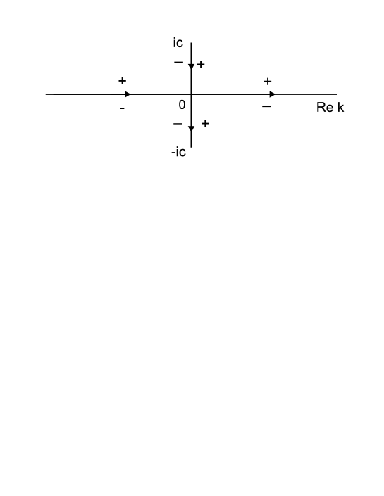
Figure 1: The oriented contour $\Sigma$

Let us define the oriented contour $\Sigma=\mathbb{R}\cup[ic,-ic]$ as on the figure 1. Then the matrix $M(\xi,t,k)$ solves the next Riemann–Hilbert problem:

• matrix valued function $M(\xi,t,k)$ is analytic in the domain $\mathbb{C}\setminus\Sigma$;

• $M(\xi,t,k)$ is bounded in neighborhoods of the end points $ic$ and $-ic$;

• $M_{-}(\xi,t,k)=M_{+}(\xi,t,k)J(\xi,t,k),\quad k\in\Sigma=\mathbb{R}\cup[ic,-ic]$, where
  
  

  $$J(\xi,t,k)=\begin{cases}\left(\begin{array}[]{ccc}1&-\overline{r(k)}e^{-2it\theta(k,\xi)}\\ \\ -r(k)e^{2it\theta(k,\xi)}&1+|r(k)|^{2}\end{array}\right),\quad k\in\mathbb{R}\backslash\{0\}\\ \\ \left(\begin{array}[]{ccc}1&0\\ \\ f(k)e^{2it\theta(k,\xi)}&1\end{array}\right),\quad k\in[0,ic]\\ \\ \left(\begin{array}[]{ccc}1&f(k)e^{-2it\theta(k,\xi)}\\ \\ 0&1\end{array}\right),\quad k\in[0,-ic]\end{cases}$$ (2.4)

• $M(\xi,t,k)=I+O(k^{-1}),\quad k\to\infty;$

where $r(k)={b(k)}/{a(k)}$, $k\in\mathbb{R}$ is given in (2.2), and

$$f(k):=f_{1}(k)=f_{2}(k)=\displaystyle\frac{\mathrm{i}}{a_{-}(k)a_{+}(k)}=\displaystyle\frac{\mathrm{i}}{\overline{a_{-}(\overline{k})}\ \overline{a_{+}(\overline{k})}}\ ,\quad k\in[ic,-ic].$$

If the initial datum is a generic step-like function then $a(k)$ can have zeroes in the domain of analyticity. In this case the matrix $M(\xi,t,k)$ will be meromorphic and residue relations between columns of the matrix $M(\xi,t,k)$ must be added.

Now we forget about the origin of the Riemann-Hilbert problem and suppose that the oriented contour $\Sigma$ and functions (2.2) are given. The following theorem take place.

Theorem 2.1.

Let the oriented contour $\Sigma$ and functions (2.2) with

$$\varkappa(k)=\sqrt[4]{\frac{k-ic}{k+ic}}$$

be given. Then the Riemann-Hilbert problem has a unique solution $M(\xi,t,k)$. The function $q(x,t)$, given by the equations,

$$q(x,t)=2\mathrm{i}\lim\limits_{k\to\infty}[kM(x/12t,t,k)]_{12},$$ (2.5)

satisfy the MKdV equation (1.1) and the initial condition

$$q(x,0)=q_{0}(x)=\begin{cases}0,\qquad x\geq 0\\ c,\qquad x<0.\end{cases}$$

The proof of this theorem almost the same as in [14], if we takes into account that given functions $a(k)$, $b(k)$ via the function $\varkappa(k)$ are in the one-to-one correspondence with the shock function $q_{0}(x)$.

3 Long time asymptotic analysis of the Riemann–Hilbert problem

3.1 Steadiness region $x<-6c^{2}t$

The jump matrices $J(\xi,t,k)$ depend on $\exp\{\pm 2\mathrm{i}t\theta(k,\xi)\}$. Hence the signature table of the imaginary part of $\theta(k,\xi)$ plays a very important role as the phase function. The stationary points of the phase function $\theta(k,\xi)$ equal to $\pm\sqrt{-\xi}$ and hence they are real because $\xi<0$. The signature table of the function

$$\operatorname{Im}\theta(k,\xi)=(12\operatorname{Re}^{2}k-4\operatorname{Im}^{2}k+12\xi)\operatorname{Im}k$$

depictured on the figure 2.

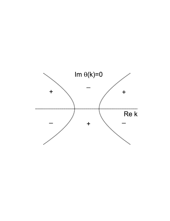
Figure 2: The signature table of the function $\operatorname{Im}\theta(k)$

Thus $\operatorname{Im}\theta(k,\xi)>0$ ($\operatorname{Im}\theta(k,\xi)<0$) for $k$ lying in the exterior (interior) of the hyperbola $3\operatorname{Re}^{2}k-\operatorname{Im}^{2}k+3\xi=0$ of the upper half-plane and in the interior (exterior) of the same hyperbola of the lower half-plane. For $\xi<0$ $\operatorname{Im}\theta(k,\xi)$ is negative along $(0,ic)$ and positive along $(0,-ic)$. Therefore the jump matrices $J(\xi,t,k)$ are unbounded (in $t$) when $k\in(-ic,ic)$. Hence we have to use the modified nonlinear steepest descent method, suggested in [2], [3], [17], and find a new phase function $g_{c}(k,\xi)$, instead of the function $\theta(k,\xi)$, which transforms the original Riemann-Hilbert problem to the model RH problem of the finite-gap type. New $g$-function leads to the finite-gap model problems of zero genus for $\xi<\xi_{-}=-c^{2}/2$ and genus one for $\xi_{-}<\xi<\xi_{+}=c^{2}/3$. They are explicitly solved by using elementary functions in the first region and the elliptic theta functions in the second region, respectively.

In the region $\xi<\xi_{-}$ we shall use the following $g$-function:

$$g_{c}(k,\xi)=\Omega(k)+12\xi X(k)=(4k^{2}-2c^{2}+12\xi)X(k)$$ (3.6)

where $X(k)=\sqrt{(k-ic)(k+ic)}=\sqrt{k^{2}+c^{2}}$. This function has the asymptotic behavior similar to the phase function $\theta(k,\xi)$, i.e.

$$g(k,\xi)=4k^{3}+12\xi k+O(k^{-1}),\qquad k\to\infty.$$

The differential of this function can be written in the form:

$$dg_{c}(k,\xi)=\frac{12k^{3}+(6c^{2}+12\xi)k}{X(k)}dk=\displaystyle\frac{(k+\lambda)k(k-\lambda)}{X(k)}dk,$$

where, evidently, $\lambda(\xi)=\sqrt{-\xi-c^{2}/2}$. In order to define the boundary value $\xi_{-}$ we take into account that the phase function $g_{c}(k,\xi)$ is acceptable until zeroes $-\lambda(\xi)$ and $\lambda(\xi)$ are different. When they coincide (are equal to zero ) and become complex conjugated then $g_{c}(k,\xi)$ does not work and new phase function must be introduced. Hence we have to put $\lambda(\xi_{-})=0$. Then $\xi_{-}=-c^{2}/2$, that gives $x<-6c^{2}t$, and the phase function $g_{c}(k,\xi)$ will be useful for $\-\infty<\xi<\xi_{-}$.

In what follows very important role plays a signature table of the function $\operatorname{Im}g_{c}(k,\xi)$ for different values of $\xi$. Borderlines between different domains are described by equations:

$$k_{2}=0;\qquad\qquad k_{1}=0\qquad\rm{and}\qquad|k_{2}|\leq c;$$

$$3\left(k_{1}^{2}-k_{2}^{2}+\xi+\frac{c^{2}}{2}\right)\left(k_{1}^{2}-k_{2}^{2}+3\xi-\frac{c^{2}}{2}\right)=4k_{1}^{2}k_{2}^{2},$$

which are equivalent to $\operatorname{Im}g_{c}(k,\xi)=0$. The signature table of the function $\operatorname{Im}g_{c}(k,\xi)$ can be obtain by using for example ”MAPLE” and it is qualitatively depicted on the figure 3 for $-\infty<\xi<\xi_{-}$ and on the figure 4 for $\xi=\xi_{-}$.

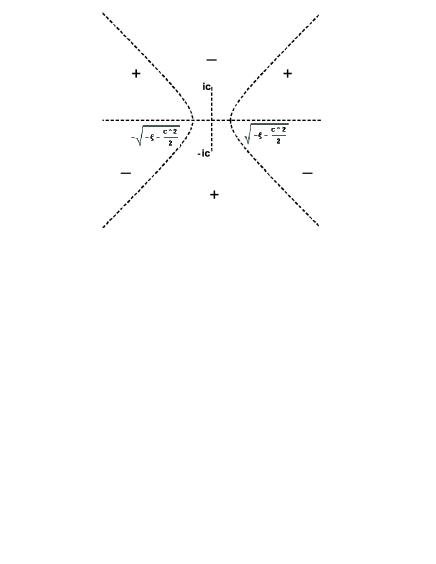
Figure 3: The signature table of the function $\operatorname{Im}g_{c}(k,\xi)$ ($\xi<\xi_{-}$)

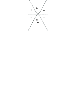
Figure 4: The signature table of the function $\operatorname{Im}g_{c}(k,\xi)$ ($\xi=\xi_{-}$)

Thus $g_{c}(k,\xi)$ as the function on $k$ has the following properties:

• $g_{c}(k,\xi)$ is analytic in $\mathbb{C}\backslash[-ic,ic]$

• $g_{c}(k,\xi)=\theta(k,\xi)+\mathrm{O}\left(k^{-1}\right),\quad k\rightarrow\infty$

• $g_{c}^{+}(k,\xi)+g_{c}^{-}(k,\xi)=0,\quad k\in(-ic,ic)$

• $g_{c}(k,\xi)=\mathrm{O}(\sqrt{k\mp ic})$, $k\to\pm ic$.

The Riemann-Hilbert problem for the matrix $M(\xi,t,k)$ with the jump contour $\Sigma=\mathbb{R}\cup[ic,-ic]$ have to be considered now with new (3.6) phase function $g_{c}(k,\xi)$. Let us define new matrix function

$$M^{(1)}(\xi,t,k)=M(\xi,t,k)G^{(1)}(\xi,t,k),$$

where $G^{(1)}(\xi,t,k)=e^{it(g_{c}(k,\xi)-\theta(k,\xi))\sigma_{3}}.$ The function $M^{(1)}$ solve the following R-H problem:

$$M^{(1)}_{-}(\xi,t,k)=M^{(1)}_{+}(\xi,t,k)J^{(1)}(\xi,t,k),\qquad M^{(1)}(\xi,t,k)\rightarrow I,\quad k\rightarrow\infty$$

where

$$J^{(1)}(\xi,t,k)=\begin{cases}\left(\begin{array}[]{ccc}1&-\overline{r(k)}e^{-2itg_{c}(k,\xi)}\\ \\ -r(k)e^{2itg_{c}(k,\xi)}&1+|r(k)|^{2}\end{array}\right),\quad k\in\mathbb{R}\\ \\ \left(\begin{array}[]{ccc}1&0\\ \\ f(k)e^{2itg_{c}(k,\xi)}&1\end{array}\right),\quad k\in(0,ic)\\ \\ \left(\begin{array}[]{ccc}1&f(k)e^{-2itg_{c}(k,\xi)}\\ \\ 0&1\end{array}\right),\quad k\in(-ic,0)\end{cases}$$

Further we would like to transfer the jump contour from the real axis. To do so we use the following factorizations of the jump matrix on the real axis:

$$J^{(1)}(\xi,t,k) =\left(\begin{array}[]{ccc}1&0\\ \\ -r(k)e^{2itg_{c}(k,\xi)}&1\end{array}\right)\left(\begin{array}[]{ccc}1&-\overline{r(k)}e^{-2itg_{c}(k,\xi)}\\ \\ 0&1\end{array}\right)$$ (3.13)

$$=\left(\begin{array}[]{ccc}1&\displaystyle\frac{-\overline{r(\overline{k})}e^{-2itg_{c}(k,\xi)}}{1+r(k)\overline{r(\overline{k})}}\\ \\ 0&1\end{array}\right)\left(\begin{array}[]{ccc}\displaystyle\frac{1}{1+|r(k)|^{2}}&0\\ \\ 0&1+|r(k)|^{2}\end{array}\right)\left(\begin{array}[]{ccc}1&0\\ \\ \displaystyle\frac{-r(k)e^{2itg_{c}(k,\xi)}}{1+r(k)\overline{r(\overline{k})}}&1\end{array}\right)$$ (3.23)

It is easy to see, the first(second) factor in the first line (3.13) is decrease as $t\rightarrow\infty$ in the domains where $\mathrm{Im}\ g_{c}(k,\xi)>0$ $(\mathrm{Im}\ g_{c}(k,\xi)<0)$. In the second line (3.23) the first(third) factor is decrease as $t\rightarrow\infty$ in the domains where $\mathrm{Im}\ g_{c}(k,\xi)<0$ $(\mathrm{Im}\ g_{c}(k,\xi)>0)$. To remove the diagonal terms in the second factorization we use a diagonal transformation:

$$M^{(2)}(\xi,t,k)=M^{(1)}(\xi,t,k)\delta^{-\sigma_{3}}(k,\xi),\qquad\delta^{-\sigma_{3}}(k,\xi)=\begin{pmatrix}\delta^{-1}(k,\xi)&0\\ 0&\delta(k,\xi)\end{pmatrix},$$

where some analytic in $\mathbb{C}\backslash[-\lambda(\xi),\lambda(\xi)]$ function $\delta(k,\xi)$ must be defined. Then the jump matrix $J^{(2)}(\xi,t,k)$ for $k\in[-\lambda(\xi),\lambda(\xi)]$ takes the form

$$J^{(2)}(\xi,t,k)=\begin{pmatrix}1&\displaystyle\frac{-\overline{r}\delta_{+}^{2}e^{-2itg_{c}(k,\xi)}}{1+|r|^{2}}\\ \\ 0&1\end{pmatrix}\begin{pmatrix}\displaystyle\frac{\delta_{+}}{\delta_{-}}(1+|r|^{2})^{-1}&0\\ 0&\displaystyle\frac{\delta_{-}}{\delta_{+}}\left(1+|r|^{2}\right)\end{pmatrix}\begin{pmatrix}1&0\\ \\ \displaystyle\frac{-re^{2itg_{c}(k,\xi)}}{(1+|r|^{2})\delta_{-}^{2}}&1\end{pmatrix}.$$

If we chose the function $\delta(k,\xi)$ in the form:

$$\delta(k,\xi)=\left(\displaystyle\frac{k-\lambda(\xi)}{k+\lambda(\xi)}\right)^{-i\nu}\chi(k,\xi),$$ (3.24)

where

$$\chi(k,\xi)=\exp\left(\displaystyle\frac{1}{2\pi i}\displaystyle\int\limits_{-\lambda(\xi)}^{\lambda(\xi)}\displaystyle\frac{\ln\left(\displaystyle\frac{1+|r(s)|^{2}}{1+|r(d)|^{2}}\right)ds}{s-k}\right)$$ (3.25)

and

$$\nu=\displaystyle\frac{1}{2\pi}\ln(1+|r(\lambda(\xi))|^{2})$$ (3.26)

then $\delta_{+}=\delta_{-}(1+|r|^{2})$ and, therefore, the middle matrix factor become trivial. Thus the jump matrix $J^{(2)}(\xi,t,k)$ has a lower/upper factorization for $k\in[-\lambda(\xi),\lambda(\xi)]$ and a upper/lower factorization for $k\notin[-\lambda(\xi),\lambda(\xi)]$:

$$J^{(2)}(\xi,t,k)=\begin{cases}\begin{pmatrix}1&a(k)b(k)\delta^{2}_{+}(k,\xi)\mathrm{e}^{-2\mathrm{i}tg_{c}(k,\xi)}\\ 0&1\end{pmatrix}\begin{pmatrix}1&0\\ -a(k)b(k)\delta^{-2}_{-}(k,\xi)\mathrm{e}^{2\mathrm{i}tg_{c}(k,\xi)}&1\end{pmatrix},\\ \hfill k\in[-\lambda(\xi),\lambda(\xi)]\\ \\ \begin{pmatrix}1&0\\ -r(k)\delta^{-2}(k,\xi)\mathrm{e}^{2\mathrm{i}tg_{c}(k,\xi)}&1\end{pmatrix}\begin{pmatrix}1&r(k)\delta^{2}(k)\mathrm{e}^{-2\mathrm{i}tg_{c}(k,\xi)}\\ 0&1\end{pmatrix},\qquad k\notin[-\lambda(\xi),\lambda(\xi)],\end{cases}$$

where we use the identity:

$$\frac{r(k)}{1+|r(k)|^{2}}=a(k)b(k).$$

For $k\in[-ic,ic]$ the jump matrix $J^{(2)}(\xi,t,k)$ takes the form:

$$\begin{pmatrix}\mathrm{e}^{-\mathrm{i}t(g^{+}_{c}(k,\xi)-g^{-}_{c}(k,\xi))}&0\\ f(k)\mathrm{e}^{\mathrm{i}t(g^{+}_{c}(k,\xi)+g^{-}_{c}(k,\xi))}&\mathrm{e}^{\mathrm{i}t(g^{+}_{c}(k,\xi)-g^{-}_{c}(k,\xi))}\end{pmatrix}, \qquad k\in[0,ic],$$

$$\begin{pmatrix}\mathrm{e}^{-\mathrm{i}t(g^{+}_{c}(k,\xi)-g^{-}_{c}(k,\xi))}&f(k)\mathrm{e}^{-\mathrm{i}t(g^{+}_{c}(k,\xi)+g^{-}_{c}(k,\xi))}\\ 0&\mathrm{e}^{\mathrm{i}t(g^{+}_{c}(k,\xi)-g^{-}_{c}(k,\xi))}\end{pmatrix}, \qquad k\in[-ic,0].$$

To remove unbounded in $t$ exponentials we have to put

$$g_{c}^{-}(k,\xi)+g_{c}^{+}(k,\xi)=0,\qquad k\in[-ic,ic].$$ (3.27)

Chosen above function $g_{c}(k,\xi)$ satisfies this condition and the jump matrix takes the form

$$J^{(2)}(\xi,t,k) =\begin{pmatrix}\mathrm{e}^{-2\mathrm{i}tg_{c}^{+}(k,\xi)}&0\\ f(k)\delta^{-2}(k)&\mathrm{e}^{2\mathrm{i}tg_{c}^{+}(k,\xi)}\end{pmatrix},\qquad k\in[ic,0]$$

$$=\begin{pmatrix}\mathrm{e}^{-2\mathrm{i}tg_{c}^{+}(k,\xi)}&f(k)\delta^{2}(k)\\ 0&\mathrm{e}^{2\mathrm{i}tg_{c}^{+}(k,\xi)}\end{pmatrix},\qquad k\in[0,ic]$$

on the contour $[ic,-ic]$. The jump contour $\Sigma^{(2)}$ for $M^{(2)}(\xi,t,k)$-problem is the initial one, i.e. $\Sigma^{(2)}=\Sigma$.

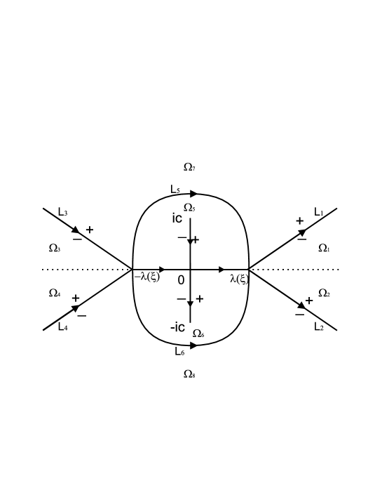
Figure 5: The contour $\Sigma^{(3)}$ for the $M^{(3)}(\xi,t,k)$-problem

Let us define a decomposition of the complex $k$-plane into eight domains $\Omega_{1},....,\Omega_{8}$ separated by their common boundary $\Sigma^{(3)}$ as it is shown on the figure 5. The contours $L_{1}$, $L_{6}$ ($L_{3}$, $L_{4}$) range from the point $\lambda(\xi)$ ($-\lambda(\xi$)) to infinity along the rays $\arg k=\pm\pi/4$ ($\arg k=\pi\mp\pi/4$); the contours $L_{2}$ and $L_{5}$, passing through the points $\pm\lambda(\xi)$, form a closed oval containing segment $[-ic,ic]$. Then the next transformation is:

$$M^{(3)}(\xi,t,k)=M^{(2)}(\xi,t,k)G^{(2)}(\xi,t,k),$$

where

$$G^{(2)}(\xi,t,k)=\begin{cases}\begin{pmatrix}1&0\\ -r(k)\delta^{-2}(k,\xi)\mathrm{e}^{2\mathrm{i}tg_{c}(k,\xi)}&1\end{pmatrix},&k\in\Omega_{1}\cup\Omega_{3},\\ \\ \begin{pmatrix}1&0\\ 0&1\end{pmatrix},&k\in\Omega_{2}\cup\Omega_{5},\\ \\ \begin{pmatrix}1&-r(k)\delta^{2}(k,\xi)\mathrm{e}^{-2\mathrm{i}tg_{c}(k,\xi)}\\ 0&1\end{pmatrix},&k\in\Omega_{4}\cup\Omega_{6},\end{cases}$$ (3.28)

$$G^{(2)}(\xi,t,k)=\begin{cases}\begin{pmatrix}1&a(k)b(k)\delta^{2}(k,\xi)\mathrm{e}^{-2\mathrm{i}tg_{c}(k,\xi)}\\ 0&1\end{pmatrix},&k\in\Omega_{7},\\ \\ \begin{pmatrix}1&0\\ a(k)b(k)\delta^{-2}(k,\xi)\mathrm{e}^{2\mathrm{i}tg_{c}(k,\xi)}&1\end{pmatrix},&k\in\Omega_{8}.\end{cases}$$ (3.29)

The $G^{(2)}$-transformation gives to the following RH problem:

$$M^{(3)}_{-}(\xi,t,k)=M^{(3)}_{+}(\xi,t,k)J^{(3)}(\xi,t,k),\qquad M^{(3)}_{-}(\xi,t,k)=I+\mathrm{O}(k^{-1}),\quad k\to\infty$$

on the contour $\Sigma^{(3)}$ depicted on the Figure 5 with jump matrices $J^{(3)}(\xi,t,k)$ which are equal to the identity matrix on the real axis, they coincide with matrices $G^{(2)}(k)$ from (3.28)-(3.29) written for the contours $k\in L_{j}$ ($j=1,2,...,6$). It is easy to see that $J^{(3)}(\xi,t,k)=I+O(\mathrm{e}^{-\epsilon t})$ as $t\to\infty$ and $k\in L_{j}$ with exception of some neighborhoods of the stationary points $\pm\lambda(\xi)$. Therefore the main contribution to the asymptotics comes from the jump matrix on the segment $[ic,-ic]$, where it takes the form:

$J^{(3)}(\xi,t,k)={G^{(2)}_{+}}^{-1}(k)J^{(2)}(\xi,t,k){G^{(2)}_{-}}(k)=$

$$= \begin{cases}\begin{pmatrix}1&-a_{+}(k)b_{+}(k)\delta^{2}(k,\xi)\mathrm{e}^{-2\mathrm{i}tg_{c}^{+}(k,\xi)}\\ 0&1\end{pmatrix}J^{(2)}(\xi,t,k)\begin{pmatrix}1&a_{-}(k)b_{-}(k)\delta^{2}(k,\xi)\mathrm{e}^{2\mathrm{i}tg_{c}^{+}(k,\xi)}\\ 0&1\end{pmatrix},\\ \hfill k\in[0,ic],\\ \\ \begin{pmatrix}1&0\\ -a_{+}(k)b_{+}(k)\delta^{-2}(k,\xi)\mathrm{e}^{2\mathrm{i}tg_{c}^{+}(k,\xi)}&1\end{pmatrix}J^{(3)}(\xi,t,k)\begin{pmatrix}1&0\\ a_{-}(k)b_{-}(k)\delta^{-2}(k,\xi)\mathrm{e}^{-2\mathrm{i}tg_{c}^{+}(k,\xi)}&1\end{pmatrix},\\ \hfill k\in[0,-ic].\end{cases}$$

Using equalities $1-f(k)a_{+}(k)b_{+}(k)=0$, $1-f(k)a_{+}(k)b_{+}(k)=0$ and $a_{+}(k)b_{+}(k)=-a_{-}(k)b_{-}(k)$, which follow from the definition of the function $f(k)$, we obtain

$$J^{(3)}(\xi,t,k)=\begin{cases}\begin{pmatrix}0&-f^{-1}(k)\delta^{2}(k,\xi)\\ f(k)\delta^{-2}(k,\xi)&0\end{pmatrix},\qquad k\in[0,ic]\\ \\ \begin{pmatrix}0&f(k)\delta^{2}(k,\xi)\\ -f^{-1}(k)\delta^{-2}(k,\xi)&0\end{pmatrix},\qquad k\in[0,-ic].\end{cases}$$

Further we would like to obtain the RH problem with constant in $k$ jump matrix. To do so let us use the factorization

$$J^{(3)}(\xi,t,k)=\begin{pmatrix}F^{-1}_{+}(k,\xi)&0\\ 0&F_{+}(k,\xi)\end{pmatrix}\begin{pmatrix}0&\mathrm{i}\\ \mathrm{i}&0\end{pmatrix}\begin{pmatrix}F_{-}(k,\xi)&0\\ 0&F^{-1}_{-}(k,\xi)\end{pmatrix}$$

which takes place if $F_{-}(k,\xi)F_{+}(k,\xi)=-\mathrm{i}f(k)\delta^{-2}(k,\xi)$ for $k\in[0,ic]$ and $F_{-}(k,\xi)F_{+}(k,\xi)=\mathrm{i}f^{-1}(k,\xi)\delta^{-2}(k,\xi)$ for $k\in[0,-ic]$.

Thus we come to the scalar Riemann-Hilbert problem: find a scalar function $F(k,\xi)$ such that

• $F(k,\xi)$ is analytic outside the contour $[ic,-ic]$ which is oriented from $ic$ to $-ic$.;

• $F(k,\xi)$ does not vanish;

• $F(k,\xi)$ satisfies the jump relation:

  $$F_{-}(k,\xi)F_{+}(k,\xi)=h(k)\delta^{-2}(k,\xi),\qquad k\in[ic,-ic],$$

  where

  $$h(k)=\begin{cases}-\mathrm{i}f(k)=a^{-1}_{-}(k)a^{-1}_{+}(k)\quad k\in[0,ic],\\ \mathrm{i}f^{-1}(k)=a_{-}(k)a_{+}(k),\quad k\in[0,-ic].\end{cases}$$

• $F(k,\xi)$ is bounded at infinity.

To solve this RH problem let us put

$$F(k,\xi)=\begin{cases}\displaystyle\frac{1}{a(k)}F_{aux}(k,\xi),\quad k\in\mathbb{C}_{+}\backslash[0,ic]\\ \\ a(k)F_{aux}(k,\xi),\quad k\in\mathbb{C}_{-}\backslash[-ic,0]\end{cases},$$ (3.30)

and use the function $X(k)=\sqrt{k^{2}+c^{2}}$. Since

$$\left[\frac{\log{F_{aux}(k,\xi)}}{X(k)}\right]_{+}-\left[\frac{\log{F_{aux}(k,\xi)}}{X(k)}\right]_{-}=\frac{\log{\delta^{-2}(k)}}{X_{+}(k)},\qquad k\in[ic,-ic],$$

and

$$\left[\frac{\log{F_{aux}(k,\xi)}}{X(k)}\right]_{+}-\left[\frac{\log{F_{aux}(k,\xi)}}{X(k)}\right]_{-}=\frac{\log{a^{2}(k)}}{X(k)},\qquad k\in\mathbb{R},$$

we have

$$F_{aux}(k,\xi)=\exp\left\{\frac{X(k)}{2\pi\mathrm{i}}\left[\int\limits_{\mathbb{R}}\frac{\log a^{2}(s)}{s-k}\frac{ds}{X(s)}-\int\limits_{-ic}^{ic}\frac{\log\delta^{-2}(s,\xi)}{s-k}\frac{ds}{X_{+}(s)}\right]\right\}.$$ (3.31)

Let us note, that $F(\infty,\xi)=1$.

Indeed, as $a(\infty)=1$ then $F(k,\infty)=F_{aux}(k,\infty)$

$$F_{aux}(\infty,\xi)=\exp\left\{\frac{-1}{2\pi\mathrm{i}}\left[\int\limits_{\mathbb{R}}\log a^{2}(s)\frac{ds}{X(s)}-\int\limits_{-ic}^{ic}\log\delta^{-2}(s,\xi)\frac{ds}{X_{+}(s)}\right]\right\}.$$ (3.32)

As

• for $s\in\mathbb{R}\quad a(s)>0\quad\&\quad a(-s)=a(s)$

• for $s\in(-ic,ic)\quad\delta(s,\xi)>0\quad\&\quad\delta(-s,\xi)=1/\delta(s,\xi)$

• for $s\in(-ic,ic)\quad X_{+}(-s)=X_{+}(s)$

then $\displaystyle\int\limits_{\mathbb{R}}\log a^{2}(s)\frac{ds}{X(s)}=0$ and $\displaystyle\int\limits_{-ic}^{ic}\log\delta^{-2}(s,\xi)\frac{ds}{X_{+}(s)}=0$

Finally, $F(\infty,\xi)=1.$

Now, since

$$J^{(3)}(\xi,t,k)=F^{-\sigma_{3}}_{+}(k,\xi)J^{mod}F^{\sigma_{3}}_{-}(k,\xi),\qquad k\in[ic,-ic],$$

where

$$J^{mod}= \begin{pmatrix}0&\mathrm{i}\\ \mathrm{i}&0\end{pmatrix}$$

the next step is as follows:

$$M^{(4)}(\xi,t,k)=M^{(3)}(\xi,t,k)F^{-\sigma_{3}}(k,\xi),\qquad$$

Then we have

$$M_{-}^{(4)}(\xi,t,k)=M_{+}^{(4)}(\xi,t,k)J^{(4)}(\xi,t,k),\qquad k\in\Sigma_{4},$$

where

$$J^{(4)}(\xi,t,k)=\begin{cases}I&k\in\mathbb{R},\\ J^{mod}&k\in(ic,-ic),\\ I+\mathrm{O}(e^{-\varepsilon t})&k\in L_{j},\quad j=1,2,...,6.\end{cases}$$

The analysis of the parametrix solutions near the end points $ic$, $-ic$ and the stationary points $\pm\lambda(\xi)$ are very similar to the analysis done in [2] and [13], respectively. In the first case, since the local representation of $g_{c}(k,\xi)$ at the points $ic$ and $-ic$ is characterized by a square root type behavior:

$$g_{c}(k,\xi)\sim g_{0}(ic,\xi)\sqrt{k-ic},\quad k\to ic;\qquad g_{c}(k,\xi)\sim\bar{g}_{0}(-ic,\xi)\sqrt{k+ic},\quad k\to-ic,$$

the relevant model Riemann-Hilbert problems are solvable in terms of the Bessel functions while in the second case of the real stationary points $\pm\lambda(\xi)$ they are solvable in terms of the parabolic cylinder functions. The contribution to the asymptotics has the order $\mathrm{O}(t^{-3/2})$ ?, $\mathrm{O}(e^{-\epsilon\sqrt{t}})$ ? in the first case and $\mathrm{O}(t^{-1/2})$ in the second case. Therefore we have:

$$M^{(4)}(\xi,t,k)=\left(I+O\left(\frac{1}{t^{1/2}}\right)\right)M^{(mod)}(k),$$ (3.33)

where $M^{(mod)}(k)$ solves the zero-gap model problem (cf. [17]):

$$M^{(mod)}_{-}(k)=M^{(mod)}_{+}(k)J^{(mod)}\qquad k\in(ic,-ic),\qquad M^{(mod)}(k)=I+\mathrm{O}(k^{-1}),\quad k\to\infty.$$

with constant jump matrix:

$$J^{mod}=\begin{pmatrix}0&\mathrm{i}\\ \mathrm{i}&0\end{pmatrix}.$$

To solve the model problem let us use the function

$$\varkappa(k)=\sqrt[4]{\displaystyle\frac{k-ic}{k+ic}}$$

introduced in the first section. Since $\varkappa_{-}(k)=\mathrm{i}\varkappa_{+}(k)$ on the cut $(ic,-ic)$ the explicit solution of the model problem takes the form:

$$M^{(mod)}(k)=\frac{1}{2}\begin{pmatrix}\varkappa(k)+\displaystyle\frac{1}{\varkappa(k)}&\varkappa(k)-\displaystyle\frac{1}{\varkappa(k)}\\ \varkappa(k)-\displaystyle\frac{1}{\varkappa(k)}&\varkappa(k)+\displaystyle\frac{1}{\varkappa(k)}\end{pmatrix}$$

Finally we have the following chain of transformations of the RH problem:

$$M(\xi,t,k)=M^{(1)}(\xi,t,k)\mathrm{e}^{\mathrm{i}t[\theta(k)-g_{c}(k,\xi)]\sigma_{3}},$$

$$M^{(1)}(\xi,t,k)=M^{(2)}(\xi,t,k)\delta^{\sigma_{3}}(k,\xi),$$

$$M^{(2)}(\xi,t,k)=M^{(3)}(\xi,t,k)[G^{(2)}(\xi,t,k)]^{-1}$$

$$M^{(3)}(x,t,k)=M^{(4)}(\xi,t,k)F^{\sigma_{3}}(k,\xi),$$

$$M^{(4)}(x,t,k)=M^{(mod)}(k)(I+O(t^{-1/2})).$$

Let us emphasize that any matrix $M^{(j)}(\xi,t,k)$ ($j=1,2,...$) defines the same functions $q(x,t)$ since all bordering matrices are diagonal at the point $k=\infty$. By the Theorem 2.1 $q(x,t)=2\mathrm{i}\lim\limits_{k\to\infty}[kM(x/12t,t,k)]_{12}$. If we denote $\lim\limits_{k\to\infty}[kM^{(j)}(x/12t,t,k)]_{12}=m^{(j)}_{12}(x,t)$ then, take into account the chain of our transformations and using the equalities $m^{mod}_{12}(x,t)=c/2\mathrm{i}$, $F(\infty,\xi)=1$, we have:

$$q(x,t) =2\mathrm{i}m_{12}(x,t)=2\mathrm{i}m^{(1)}_{12}(x,t)=2\mathrm{i}m^{(2)}_{12}(x,t)$$

$$=2\mathrm{i}m^{(3)}_{12}(x,t)+\mathrm{O}(t^{-1/2})$$

$$=2\mathrm{i}m^{(4)}_{12}(x,t)F^{-2}(\infty,\xi)+\mathrm{O}(t^{-1/2})$$

$$=2\mathrm{i}m^{mod}_{12}(x,t)F^{-2}(\infty,\xi)+\mathrm{O}(t^{-1/2})$$

$$=c+\mathrm{O}(t^{-1/2}).$$

Theorem 3.1.

The solution of the IBV problem (1.1)-(1.2) for $t\to\infty$ in the region $-\infty<x<-6c^{2}t$ takes the form:

$$q(x,t) = c+O(t^{-1/2}),$$

3.2 Elliptic-wave region $-6c^{2}t<x<4c^{2}t$

3.2.1 The construction of the $g$-function

We need a function $g(k,\xi)$ with the following properties:

1. g is analytic against k in $\mathbb{C}\backslash[-ic,ic]$

2. $\exists\lim\limits_{k\rightarrow\infty}(g(k,\xi)-\theta(k,\xi))\in\mathbb{C}$

3. a set of points where $\mathrm{Im}\ g(k,\xi)=0$ divides the complex plane into four connected open sets and contains the set $\mathbb{R}\bigcup[ic,id]\bigcup[-ic,-id]$, where $d\in(0,c)$ is some number.

We will find such a function in the form:

$$g(k,\xi)=\int\limits_{ic}^{k}\frac{12(s^{2}+\mu^{2})(s^{2}+d^{2})ds}{\mathrm{w}(s)},\qquad\mathrm{w}(s)=\sqrt{(s^{2}+c^{2})(s^{2}+d^{2})},$$

where the positive on the real axis $\mathbb{R}$ function $\mathrm{w}(s)$ is analytic in $\mathbb{C}\backslash[-ic,ic]$ and numbers $\mu$ and $d$ have to be determined as functions on $\xi$. The integration contour is taken to have no intersection with the segment $(-ic,ic)$. It is easy to see that $g(k,\xi)\in\mathbb{R}$ if $k\in[c,d]_{+}$ or $k\in[c,d]_{-}$. To satisfy the requirement $g(k,\xi)\in\mathbb{R}$ if $k\in[-c,-d]_{+}$ or $k\in[-c,-d]_{-}$ we have to choose the numbers $\mu$ and $d$ in such a way that $\int\limits_{-ic}^{ic}dg(k)=0$. Besides this requirement makes $g(k,\xi)$ being a single-valued function on $\mathbb{C}\setminus[-ic,ic]$ against $k$. The mentioned requirement can be written as follows:

$$\int\limits_{0}^{1}\left(\mu^{2}-\lambda^{2}d^{2}\right)\sqrt{{\frac{1-\lambda^{2}}{c^{2}-\displaystyle{\lambda^{2}d^{2}}}}}d\lambda=0.$$ (3.34)

Let us define the function

$$F(\mu,d)=\int\limits_{0}^{1}\left(\mu^{2}-\lambda^{2}d^{2}\right)\sqrt{{\frac{1-\lambda^{2}}{c^{2}-\displaystyle{\lambda^{2}d^{2}}}}}d\lambda.$$ (3.35)

It is easy to see that there exists a function $\mu=\mu(d)$ such that $F(\mu(d),d)\equiv 0$ and $0<\mu(d)<d$. Moreover, $\mu(d)$ is strictly increasing when $d\in[0,c]$. Indeed, one can check that $F(\mu,d)$ is strictly increasing against $\mu$ and is strictly decreasing against $d$ when $0<\mu<d<c$. Now if $0<d_{1}<d_{2}<c$ then $F(\mu(d_{1}),d_{1})=0=F(\mu(d_{2}),d_{2})<F(\mu(d_{2}),d_{1})$, that is $F(\mu(d_{1}),d_{1})<F(\mu(d_{2}),d_{1})$ and, hence, $\mu(d_{1})<\mu(d_{2})$. Furthermore $\mu(d)$ is continuous function. It follows from 3.34:

$$\mu^{2}(d)=\int\limits_{0}^{1}\lambda^{2}d^{2}\sqrt{\frac{1-\lambda^{2}}{c^{2}-\lambda^{2}d^{2}}}d\lambda\Bigg{/}\int\limits_{0}^{1}\sqrt{\frac{1-\lambda^{2}}{c^{2}-\lambda^{2}d^{2}}}d\lambda$$ (3.36)

Now we want to satisfy the requirement (2) $\exists\lim\limits_{k\rightarrow\infty}(g(k,\xi)-\theta(k,\xi))\in\mathbb{C}$. For this enough that $dg(k,\xi)-d\theta(k,\xi)=\mathrm{O}(k^{-2})\quad{\rm as}\quad k\rightarrow\infty$. Since $d\theta(k,\xi)=12(k^{2}+\xi)dk$ and $dg(k,\xi)=[12(k^{2}+\mu^{2}-\displaystyle\frac{c^{2}}{2}+\displaystyle\frac{d^{2}}{2})+\mathrm{O}(k^{-2})]dk\quad{\rm as}\quad k\rightarrow\infty$, we require that

$$\frac{c^{2}}{2}+\xi=\mu^{2}+\displaystyle\frac{d^{2}}{2}.$$ (3.37)

Equation (3.36) yields that $\mu(0)=0$ and $\mu(c)=\displaystyle\frac{c}{\sqrt{3}}.$ Hence $\mu^{2}(d)+\displaystyle\frac{d^{2}}{2}$ is vary over the segment $[0,\displaystyle\frac{5c^{2}}{6}]$ when $d$ is vary over the segment $[0,c]$. So for any $\xi\in\left(-\displaystyle\frac{c^{2}}{2},\displaystyle\frac{c^{2}}{3}\right)$ there exists a single $d=d(\xi)\in(0,c)$ such that

$$\frac{c^{2}}{2}+\xi=\mu^{2}(d(\xi))+\displaystyle\frac{d(\xi)^{2}}{2}.$$ (3.38)

It is easy to see from (3.38) that $d(\xi)$ is continuous as the function on $\xi\in\left(-\displaystyle\frac{c^{2}}{2},\displaystyle\frac{c^{2}}{3}\right)$. Thus the function $g(k,\xi)$ is completely defined.

Figure 6: The signature table for Im g

The signature table of the imaginary part of the function $g(k,\xi)$ is depicted on figure 6.

The function $g(k,\xi)$ has the following additional properties:

1. $\lim\limits_{k\rightarrow\infty}\left(g(k,\xi)-\theta(k,\xi)\right)=0$
   It is follows from the facts that this limit exists and

   $$g(k,\xi)-\theta(k,\xi)\in\mathrm{i}\mathbb{R}\quad,\quad k\in(\\ ic,i\infty)$$

   and

   $$g(k,\xi)-\theta(k,\xi)\in\mathbb{R}\quad,\quad k\in\mathbb{R}$$

2. $g_{-}(k,\xi)+g_{+}(k,\xi)=0,\quad k\in(ic,id)\bigcup(-ic,-id)$;

3. $g_{-}(k,\xi)-g_{+}(k,\xi)=B_{g}(\xi)>0,\quad k\in(-id,id)$, where

   $$B_{g}(\xi)=2\int\limits_{id}^{ic}dg(k,\xi)=24\int\limits_{d}^{c}\left[\left(s^{2}-\mu^{2}(\xi)\right)\sqrt{\displaystyle\frac{s^{2}-d^{2}(\xi)}{c^{2}-s^{2}}}\right]ds=$$

   $$\hfill=24\displaystyle\int\limits_{\frac{d}{c}}^{1}\frac{\left(t^{2}-\frac{\mu^{2}(\xi)}{c^{2}}\right)\sqrt{t^{2}-\frac{d^{2}(\xi)}{c^{2}}}}{\sqrt{1-t^{2}}}dt.$$

3.2.2 Transition from initial R-H problem to the model one.

Now we introduce the chain of the transformations of the R-H problem.
Step 1
First, we change the phase function $\theta(k,\xi)$ with $g(k,\xi)$:

$$M^{(1)}(\xi,t,k)=M(\xi,t,k)e^{it(g(k,\xi)-\theta(k,\xi))\sigma_{3}}.$$

Then

$$M^{(1)}(\xi,t,k)\rightarrow I,\quad k\rightarrow\infty$$

and

$$M^{(1)}_{-}(\xi,t,k)=M^{(1)}_{+}(\xi,t,k)J^{(1)}(\xi,t,k),$$

where

$$J^{(1)}(\xi,t,k) =\left(\begin{array}[]{ccc}1&-\overline{r(k)}e^{-2itg(k,\xi)}\\ \\ -r(k)e^{2itg(k,\xi)}&1+|r(k)|^{2}\end{array}\right), k\in\mathbb{R}$$

$$=\left(\begin{array}[]{ccc}e^{itB_{g}(\xi)}&0\\ \\ f(k)e^{it(2g_{+}(k,\xi)+B_{g}(\xi))}&e^{-itB_{g}(\xi)}\end{array}\right), k\in(0,id)$$

$$=\left(\begin{array}[]{ccc}e^{itB_{g}(\xi)}&f(k)e^{-it\left(2g_{+}(k,\xi)+B_{g}(\xi)\right)}\\ \\ 0&e^{-itB_{g}(\xi)}\end{array}\right), k\in(0,-id),$$

$$=\left(\begin{array}[]{ccc}e^{-2itg_{+}(k,\xi)}&0\\ \\ f(k)&e^{2itg_{+}(k,\xi)}\end{array}\right), k\in(ic,id),$$

$$=\left(\begin{array}[]{ccc}e^{-2itg_{+}(k,\xi)}&f(k)\\ \\ 0&e^{2itg_{+}(k,\xi)}\end{array}\right), k\in(-ic,-id).$$

Step 2
The function $g(k,\xi)$ and its imaginary part (see signature table of the $\operatorname{Im}g(k,\xi)$ on the figure (6)) suggest a choice of new contour $\Sigma_{2}$ for R-H problem. Let $L_{\pm}=\{k:k=s\pm\mu(\xi),-\infty<s<\infty\}$ be the strait lines. Then $\Sigma_{2}=\mathbb{R}\cup[-ic,ic]\cup L_{+}\cup L_{-}$. We use the lower-upper factorization (3.13) of the jump matrix on the real axis and apply the transformation

$$M^{(2)}(\xi,t,k)=M^{(1)}(\xi,t,k)G^{(2)}(\xi,t,k),\qquad G^{(2)}(\xi,t,k)=\begin{cases}\left(\begin{array}[]{ccc}1&0\\ \\ -r(k)e^{2itg(k,\xi)}&1\end{array}\right),\quad k\in\Omega_{1}\\ \\ \left(\begin{array}[]{ccc}1&\overline{r(\overline{k})}e^{-2itg(k)}\\ \\ 0&1\end{array}\right),\quad k\in\Omega_{2}\\ \\ I,\quad k\in\Omega_{3}\bigcup\Omega_{4}\end{cases}$$ (3.39)

where domains $\Omega_{j},j=1,2,3,4$ are indicated on the figure (7) and get the new R-H problem:

$$\quad M^{(2)}_{-}(\xi,t,k)=M^{(2)}_{+}(\xi,t,k)J^{(2)}(\xi,t,k),$$ (3.40)

$$M^{(2)}(\xi,t,k)\rightarrow I,\quad k\rightarrow\infty$$

with the following jump matrices:

$$J^{(2)}(\xi,t,k) =\begin{pmatrix}1&0\\ \\ -r(k)\mathrm{e}^{2\mathrm{i}tg(k)}&1\end{pmatrix}, k\in L_{+},$$

$$=\begin{pmatrix}1&\bar{r}(\bar{k})\mathrm{e}^{-2\mathrm{i}tg(k,\xi)}\\ \\ 0&1\end{pmatrix}, k\in L_{-},$$

$$=\begin{pmatrix}\mathrm{e}^{\mathrm{i}tB_{g}(\xi)}&o\\ \\ 0&\mathrm{e}^{\mathrm{i}tB_{g}(\xi)}\end{pmatrix}, k\in(-id,id)$$

$$=\begin{pmatrix}\mathrm{e}^{-2\mathrm{i}tg_{+}(k,\xi)}&0\\ \\ f(k)&\mathrm{e}^{2\mathrm{i}tg_{+}(k,\xi)}\end{pmatrix}, k\in(ic,id),$$

$$=\begin{pmatrix}\mathrm{e}^{-2\mathrm{i}tg_{+}(k,\xi)}&f(k)\\ \\ 0&\mathrm{e}^{2\mathrm{i}tg_{+}(k,\xi)}\end{pmatrix}, k\in(-ic,-id).$$

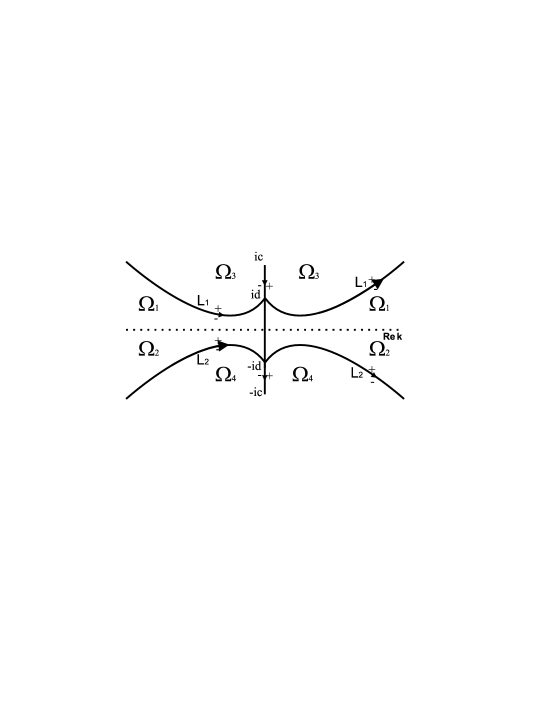
Figure 7: The contour $\Sigma_{2}$ for the R-H problem $M^{(2)}(\xi,t,k)$

We have just used the properties 1-5 of the function $g(k,\xi)$, the jump relation

$$f(k)=r_{-}(k)-r_{+}(k),\quad k\in(0,ic)$$

and symmetry relation

$$\quad r(k)=-\overline{r(\overline{k})},\quad k\in\left(\mathbb{C}\backslash(-ic,ic)\right)\\ \bigcup\left((-ic,ic)_{+}\bigcup(-ic,ic)_{-}\right).$$

Step 3
First we note that the function $f(k)$ has the following analytic continuation from the interval $(-ic,ic)$:

$$f(k)=\widehat{f}_{+}(k),\quad k\in(-ic,ic),$$ (3.41)

where

$$\widehat{f}(k)=\displaystyle\frac{4}{\varkappa^{2}(k)-\displaystyle\frac{1}{\varkappa^{2}(k)}}=\frac{2i}{c}\sqrt{k^{2}+c^{2}},\qquad\varkappa(k)=\sqrt[4]{\displaystyle\frac{k-ic}{k+ic}}.$$ (3.42)

Then we factorize the jump matrix $J^{(2)}$ on $(ic,id)\bigcup(-ic,-\mathrm{i}d)$ as follows:

$$J^{(2)}(\xi,t,k)==F_{+}^{-\sigma_{3}}(k,\xi)\begin{pmatrix}1&0\\ \\ \displaystyle\frac{e^{2itg_{+}(k,\xi)}}{\widehat{f}_{+}(k)F_{+}^{2}(k,\xi)}&1\end{pmatrix}\begin{pmatrix}0&i\\ i&0\end{pmatrix}\begin{pmatrix}1&0\\ \\ \displaystyle\frac{-e^{2itg_{-}(k,\xi)}}{\widehat{f}_{-}(k)F_{-}^{2}(k,\xi)}&1\end{pmatrix}F_{-}^{\sigma_{3}}(k,\xi),$$ (3.43)

for $k\in(ic,id)$ and

$$J^{(2)}(\xi,t,k)=F_{+}^{-\sigma_{3}}(k,\xi)\begin{pmatrix}1&\displaystyle\frac{F_{+}^{2}(k,\xi)e^{-2itg_{+}(k,\xi)}}{\widehat{f}_{+}(k)}\\ \\ 0&1\end{pmatrix}\begin{pmatrix}0&i\\ i&0\end{pmatrix}\begin{pmatrix}1&\displaystyle\frac{-F_{-}^{2}(k,\xi)e^{-2itg_{-}(k,\xi)}}{\widehat{f}_{-}(k)}\\ \\ 0&1\end{pmatrix}F_{-}^{\sigma_{3}}(k,\xi)$$ (3.44)

for $k\in(-ic,-id)$. Direct calculations show that it is possible if

• $F(k,\xi)$ is analytic outside the contour $[ic,-ic]$ which is oriented from $ic$ to $-ic$.;

• $F(k,\xi)$ does not vanish;

• $F(k,\xi)$ satisfies the jump relation:

  $$F_{-}(k,\xi)F_{+}(k,\xi)=\begin{cases}-if(k)=(a_{-}(k)a_{+}(k))^{-1},\quad k\in(ic,id)\\ \displaystyle\frac{i}{f(k)}=a_{-}(k)a_{+}(k),\quad k\in(-ic,-id),\end{cases},$$

  and

  $$F_{-}(k,\xi)=F_{+}(k,\xi)h(k),\quad k\in(-id,id),$$

  where $h(k)$ is some function, which has to be determined.

• $F(k,\xi)$ is bounded at infinity.

Figure 8: The contour $\Sigma_{3}$ for the R-H problem $M^{(3)}(\xi,t,k)$

To solve this RH problem let us put

$$F(k,\xi)=\begin{cases}\displaystyle\frac{1}{a(k)}F_{aux}(k,\xi),\quad k\in\mathbb{C}_{+}\backslash[0,ic]\\ \\ a(k)F_{aux}(k,\xi),\quad k\in\mathbb{C}_{-}\backslash[-ic,0]\end{cases},$$ (3.45)

. Since

$$F_{aux-}(k,\xi)F_{aux+}(k,\xi)=1,\quad k\in(ic,id)\bigcup(-ic,-id)$$

$$F_{aux+}(k,\xi)=F_{aux-}(k,\xi)a^{2}(k),\quad k\in\mathbb{R}$$

We use the function $\mathrm{w}(k)=\sqrt{(k^{2}+c^{2})(k^{2}+d^{2})}$.Since

$$\left[\frac{\log{F_{aux}(k,\xi)}}{\mathrm{w}(k)}\right]_{+}-\left[\frac{\log{F_{aux}(k,\xi)}}{\mathrm{w}(k)}\right]_{-}=0,\qquad k\in(ic,id)\bigcup(-ic,-id),$$

and

$$\left[\frac{\log{F_{aux}(k,\xi)}}{\mathrm{w}(k)}\right]_{+}-\left[\frac{\log{F_{aux}(k,\xi)}}{\mathrm{w}(k)}\right]_{-}=\frac{\log{a^{2}(k)}}{\mathrm{w}(k)},\qquad k\in\mathbb{R},$$

we have that one of the functions which satisfy the last two equations is

$$\widetilde{F}_{aux}(k,\xi)=\exp\left\{\frac{\mathrm{w}(k)}{2\pi\mathrm{i}}\int\limits_{\mathbb{R}}\frac{\log a^{2}(s)}{s-k}\frac{ds}{\mathrm{w}(s)}\right\}.$$ (3.46)

$$\widetilde{F}_{aux}(k,\xi)=e^{ik\Delta}\left(1+\mathrm{O}\left(\displaystyle\frac{1}{k}\right)\right),k\rightarrow\infty$$

where

$$\Delta=\displaystyle\frac{1}{2\pi}\displaystyle\int\limits_{-\infty}^{\infty}\frac{\log a^{2}(s)ds}{\mathrm{w}(s)}<0$$

But $\widetilde{F}_{aux}(k,\xi)$ has an essential singularity in infinity. To remove this singularity we introduce an Abelian integral of the second kind

$$\Omega(k)=d_{0}+\displaystyle\int\limits_{ic}^{\infty}\frac{(s^{2}+e_{0})ds}{\mathrm{w}(s)}$$

so that

$$\Omega(k)=k+\mathrm{O}\left(\displaystyle\frac{1}{k}\right),\quad k\rightarrow\infty$$

$$\int\limits_{0}^{id}\frac{(s^{2}+e_{0})ds}{\mathrm{w}(s)}=0$$

As

$$\begin{array}[]{ccc}\Omega(k)-k\in\mathbb{R},\quad k\in\mathbb{R}\\ \Omega(k)-k\in i\mathbb{R},\quad k\in i\mathbb{R}\end{array}$$ (3.47)

then $d_{0}=0$ and

$$\Omega(k)=\displaystyle\int\limits_{ic}^{\infty}\frac{(s^{2}+e_{0})ds}{\mathrm{w}(s)}$$

Then

$$\Omega_{+}+\Omega_{-}=0\quad\textrm{on}\quad(ic,id)\bigcup(-ic,-id)$$

$$\Omega_{-}-\Omega_{+}=B_{\Omega}<0\quad\textrm{on}\quad(id,-id)$$

Define

$$F_{aux}(k,\xi)=\exp\left\{\displaystyle\frac{\mathrm{w}(k)}{\pi i}\int\limits_{-\infty}^{\infty}\displaystyle\frac{\ln a(s)ds}{(s-k)\mathrm{w}(s)}-i\Delta(\xi)\Omega(k,\xi),\right\}$$ (3.48)

Then $F(k,\xi)$ defined by (3.45) has the following additional properties:

• $\lim\limits_{k\rightarrow\infty}F(k,\xi)=1,\quad k\rightarrow\infty$

• $F_{-}(k,\xi)=F_{+}(k,\xi)\displaystyle e^{-iB_{\Omega}(\xi)\Delta(\xi)},\quad k\in(-id,id),$

By using the factorizations (3.44), (3.43) we get the following RH problem:

$$M^{(3)}(\xi,t,k)=M^{(2)}(\xi,t,k)G^{(3)}(\xi,t,k),\quad M^{(3)}_{-}(\xi,t,k)=M^{(3)}_{+}(\xi,t,k)J^{(3)}(\xi,t,k),$$ (3.49)

$$M^{(3)}(\xi,t,k)\rightarrow I,\quad k\rightarrow\infty$$

where

$$G^{(3)}(\xi,t,k)=F^{-\sigma_{3}}(k,\xi)\left(\begin{array}[]{ccc}1&\displaystyle\frac{F^{2}(k,\xi)e^{-2itg(k,\xi)}}{\widehat{f}(k)}\\ \\ 0&1\end{array}\right),\quad k\in\Omega_{5}\bigcup\Omega_{7}$$ (3.50)

$$=F^{-\sigma_{3}}(k,\xi)\left(\begin{array}[]{ccc}1&0\\ \\ \displaystyle\frac{e^{2itg(k,\xi)}}{\widehat{f}(k)F^{2}(k,\xi)}&1\end{array}\right),\quad k\in\Omega_{6}\bigcup\Omega_{8}$$ (3.51)

$$=F^{-\sigma_{3}}(k,\xi),\quad k\notin\Omega_{5}\bigcup\Omega_{6}\bigcup\Omega_{7}\bigcup\Omega_{8},$$ (3.52)

and

$$J^{(3)}(\xi,t,k)=\left(\begin{array}[]{ccc}1&\displaystyle\frac{F^{2}(k,\xi)e^{-2itg(k,\xi)}}{\widehat{f}(k)}\\ \\ 0&1\end{array}\right),\quad k\in L_{7},\qquad=\left(\begin{array}[]{ccc}1&\displaystyle\frac{-F^{2}(k,\xi)e^{-2itg(k,\xi)}}{\widehat{f}(k)}\\ \\ 0&1\end{array}\right),\quad k\in L_{5}$$ (3.53)

$$=\left(\begin{array}[]{ccc}1&0\\ \\ \displaystyle\frac{e^{2itg(k,\xi)}}{\widehat{f}(k)F^{2}(k,\xi)}&1\end{array}\right),\quad k\in L_{8},\qquad=\left(\begin{array}[]{ccc}1&0\\ \\ \displaystyle\frac{e^{2itg(k,\xi)}}{\widehat{f}(k)F^{2}(k,\xi)}&1\end{array}\right),\quad k\in L_{6}$$ (3.54)

$$=\left(\begin{array}[]{ccc}1&0\\ \\ \displaystyle\frac{-r(k)e^{2itg(k,\xi)}}{F^{2}(k,\xi)}&1\end{array}\right),\quad k\in L_{1}\qquad=\left(\begin{array}[]{ccc}1&\displaystyle\frac{-\overline{r(\overline{k})}F^{2}(k,\xi)}{e^{2itg(k,\xi)}}\\ \\ 0&1\end{array}\right),\quad k\in L_{2}$$ (3.55)

$$=e^{(itB_{g}(\xi)+iB_{\Omega}(\xi)\Delta(\xi))\sigma_{3}},\quad k\in(-id,id)\qquad=\left(\begin{array}[]{ccc}0&i\\ i&0\end{array}\right),\quad k\in(ic,id)\bigcup(-id,-ic)$$ (3.56)

Step 4
Now we introduce a model problem $M^{(mod)}_{-}=M^{(mod)}_{+}J^{(mod)},\quad M^{(mod)}\rightarrow I\quad\textrm{as}\quad k\rightarrow\infty,\quad$ where

$$J^{(mod)}(\xi,t,k)=\begin{cases}e^{(itB_{g}(\xi)+iB_{\Omega}(\xi)\Delta(\xi))\sigma_{3}},\quad k\in(-id,id)\\ \\ \left(\begin{array}[]{ccc}0&i\\ i&0\end{array}\right),\quad k\in(ic,id)\bigcup(-id,-ic)\end{cases}$$ (3.57)

To solve it we need a notion of the Riemann surface $X$, which is induced by

$$\mathrm{w}^{2}(k)=(k^{2}+d^{2})(k^{2}+d^{2}),$$

with cuts along $(ic,id)$ and $(-id,-ic)$. On the first sheet of this surface $\mathrm{w}(0)>0$. We introduce the a-cycle and the b-cycle as it is shown at the picture:
The basic of the holomorphic differential forms is given by the differential form

$$\omega=2\pi i\displaystyle\frac{\displaystyle\frac{dk}{\mathrm{w}(k)}}{\displaystyle\int\limits_{a}\displaystyle\frac{dk}{\mathrm{w}(k)}}.$$

Then

$$\int\limits_{a}\displaystyle\frac{dk}{\mathrm{w}(k)}=2\pi i$$

$$\tau=\tau(\xi):=\displaystyle\int\limits_{b}\displaystyle\frac{dk}{\mathrm{w}(k)}<0$$

We introduce the Poincare theta function:

$$\Theta(z)=\Theta(z,\tau(\xi))=\sum\limits_{m=-\infty}^{\infty}\exp\left\{\displaystyle\frac{1}{2}\tau(\xi)m^{2}+zm\right\}$$

It has the following property:

$$\Theta(z+2\pi in+\tau(\xi)l,\tau(\xi))=\Theta(z,\tau(\xi))\exp\left\{-\displaystyle\frac{1}{2}\tau(\xi)l^{2}-zl\right\},\quad n\in\mathbb{N},l\in\mathbb{N}$$ (3.58)

Then we introduce the Abel mapping on the surface $X$:

$$A:X\rightarrow\mathbb{C}/\left(2\pi i\mathbb{Z}+\tau(\xi)\mathbb{Z}\right)\qquad A(P)=\int\limits_{ic}^{P}\omega$$

Now we introduce the functions $\varphi(.,\xi),\psi(.,\xi):\{\textrm{the first sheet of the X}\}\rightarrow\mathbb{C}$

$$\begin{array}[]{l}\varphi_{j}(k,\xi)=\displaystyle\frac{\Theta(A(k)-A(D_{j})-K-itB_{g}(\xi)-iB_{\Omega}\Delta(\xi))}{\Theta(A(k)-A(D_{j})-K)}\\ \\ \psi_{j}(k,\xi)=\displaystyle\frac{\Theta(-A(k)-A(D_{j})-K-itB_{g}(\xi)-iB_{\Omega}\Delta(\xi))}{\Theta(-A(k)-A(D_{j})-K)}\end{array},\quad j=\displaystyle\overline{1,2},$$ (3.59)

where $D_{1}=(0,-cd)$ is on the second sheet and $D_{1}=(0,cd)$ is on the first sheet. $A(D_{1})=-A(D_{2}).$ $K$ is the Riemann constant of the surface $X$. The integration contour in (3.59) is taken on the first sheet and not to intersect the interval(-ic,ic). These functions have the following properties:

$$\begin{array}[]{l}\varphi_{+}(k,\xi)=\psi_{-}(k,\xi)\\ \\ \psi_{+}(k,\xi)=\varphi_{-}(k,\xi)\end{array},\quad k\in(ic,id)\bigcup(-id,-ic)$$

$$\begin{array}[]{l}\varphi_{-}(k,\xi)=\varphi_{+}(k,\xi)e^{itB_{g}(\xi)+iB_{\Omega}\Delta(\xi)}\\ \\ \psi_{-}(k,\xi)=\psi_{+}(k,\xi)e^{-itB_{g}(\xi)-iB_{\Omega}\Delta(\xi)}\end{array},\quad k\in(id,-id)$$

Define a function

$$\gamma(k)=\gamma(k,\xi)=\left(\displaystyle\frac{k-ic}{k-id}\right)^{\displaystyle\frac{1}{4}}\left(\displaystyle\frac{k+id}{k+ic}\right)^{\displaystyle\frac{1}{4}}$$

Then the solution of the model problem of the 4 can be produce as following:

$$M^{(mod)}(\xi,t,k)=\left(\begin{array}[]{ccc}M^{(mod)}_{11}(\xi,t,k)&M^{(mod)}_{12}(\xi,t,k)\\ \\ M^{(mod)}_{21}(\xi,t,k)&M^{(mod)}_{22}(\xi,t,k)\end{array}\right)$$ (3.60)

$$\hfill M^{(mod)}(\xi,t,k)=$$ (3.61)

$${}\left(\begin{array}[]{ccc}\varphi_{1}^{-1}(\infty,\xi)&0\\ 0&\varphi_{2}^{-1}(\infty,\xi)\end{array}\right)\left(\begin{array}[]{ccc}\displaystyle\frac{\gamma(k,\xi)+\displaystyle\frac{1}{\gamma(k,\xi)}}{2}\varphi_{1}(k,\xi)&\displaystyle\frac{\gamma(k,\xi)-\displaystyle\frac{1}{\gamma(k,\xi)}}{2}\psi_{1}(k,\xi)\\ \\ \displaystyle\frac{\gamma(k,\xi)-\displaystyle\frac{1}{\gamma(k,\xi)}}{2}\varphi_{2}(k,\xi)&\displaystyle\frac{\gamma(k,\xi)+\displaystyle\frac{1}{\gamma(k,\xi)}}{2}\psi_{2}(k,\xi)\end{array}\right)$$ (3.62)

Let us note that

$$A(\infty)=\displaystyle\frac{\pi i}{2}$$

$$K=\displaystyle\frac{\pi i}{2}+\displaystyle\frac{\tau}{2}$$

$$A(0_{\pm})=\mp\displaystyle\frac{\tau}{2}+\displaystyle\frac{\pi i}{2}$$

Taking it in (3.62) we have:

$${}\hfill M^{(mod)}(\xi,t,k)=\left(\begin{array}[]{ccc}\left(M^{(mod)}(\xi,t,k)\right)_{11}&\left(M^{(mod)}(\xi,t,k)\right)_{12}\\ \left(M^{(mod)}(\xi,t,k)\right)_{21}&\left(M^{(mod)}(\xi,t,k)\right)_{22}\end{array}\right)$$ (3.63)

and

$${}\left(M^{(mod)}(\xi,t,k)\right)_{11}=\displaystyle\frac{\left(\gamma+\displaystyle\frac{1}{\gamma}\right)}{2}\displaystyle\frac{\Theta(A(P)-\displaystyle\frac{\pi i}{2}-itB_{g}-iB_{\Omega}\Delta)}{\Theta(A(P)-\displaystyle\frac{\pi i}{2})}\frac{\Theta(0)}{\Theta(itB_{g}+B_{\Omega}\Delta)}$$ (3.64)

$${}\left(M^{(mod)}(\xi,t,k)\right)_{12}=\displaystyle\frac{\left(\gamma-\displaystyle\frac{1}{\gamma}\right)}{2}\displaystyle\frac{\Theta(-A(P)-\displaystyle\frac{\pi i}{2}-itB_{g}-iB_{\Omega}\Delta)}{\Theta(-A(P)-\displaystyle\frac{\pi i}{2})}\frac{\Theta(0)}{\Theta(itB_{g}+B_{\Omega}\Delta)}$$ (3.65)

$${}\left(M^{(mod)}(\xi,t,k)\right)_{21}=\displaystyle\frac{\left(\gamma-\displaystyle\frac{1}{\gamma}\right)}{2}\displaystyle\frac{\Theta(A(P)+\displaystyle\frac{\pi i}{2}-itB_{g}-iB_{\Omega}\Delta)}{\Theta(A(P)+\displaystyle\frac{\pi i}{2})}\frac{\Theta(0)}{\Theta(itB_{g}+B_{\Omega}\Delta)}$$ (3.66)

$${}\left(M^{(mod)}(\xi,t,k)\right)_{22}=\displaystyle\frac{\left(\gamma+\displaystyle\frac{1}{\gamma}\right)}{2}\displaystyle\frac{\Theta(-A(P)+\displaystyle\frac{\pi i}{2}-itB_{g}-iB_{\Omega}\Delta)}{\Theta(-A(P)+\displaystyle\frac{\pi i}{2})}\frac{\Theta(0)}{\Theta(itB_{g}+B_{\Omega}\Delta)}$$ (3.67)

We can also solve the model problem by using a function

$$\lambda(k)=\sqrt[4]{\frac{k-ic}{k+ic}}\sqrt[4]{\frac{k-id}{k+id}}$$

Then we have that

$${}\hfill M^{(mod)}(\xi,t,k)=\left(\begin{array}[]{ccc}\left(M^{(mod)}(\xi,t,k)\right)_{11}&\left(M^{(mod)}(\xi,t,k)\right)_{12}\\ \left(M^{(mod)}(\xi,t,k)\right)_{21}&\left(M^{(mod)}(\xi,t,k)\right)_{22}\end{array}\right)$$ (3.68)

$${}\left(M^{(mod)}(\xi,t,k)\right)_{11}=\displaystyle\frac{\left(\lambda+\displaystyle\frac{1}{\lambda}\right)}{2}\displaystyle\frac{\Theta(A(P)-\displaystyle\frac{\pi i}{2}-itB_{g}-iB_{\Omega}\Delta)}{\Theta(A(P)+\displaystyle\frac{\pi i}{2})}\frac{\Theta(\pi i)}{\Theta(itB_{g}+B_{\Omega}\Delta)}$$ (3.69)

$${}\left(M^{(mod)}(\xi,t,k)\right)_{12}=\displaystyle\frac{\left(\lambda-\displaystyle\frac{1}{\lambda}\right)}{2}\displaystyle\frac{\Theta(-A(P)-\displaystyle\frac{\pi i}{2}-itB_{g}-iB_{\Omega}\Delta)}{\Theta(-A(P)+\displaystyle\frac{\pi i}{2})}\frac{\Theta(\pi i)}{\Theta(itB_{g}+B_{\Omega}\Delta)}$$ (3.70)

$${}\left(M^{(mod)}(\xi,t,k)\right)_{21}=\displaystyle\frac{\left(\lambda-\displaystyle\frac{1}{\lambda}\right)}{2}\displaystyle\frac{\Theta(A(P)+\displaystyle\frac{\pi i}{2}-itB_{g}-iB_{\Omega}\Delta)}{\Theta(A(P)-\displaystyle\frac{\pi i}{2})}\frac{\Theta(\pi i)}{\Theta(itB_{g}+B_{\Omega}\Delta)}$$ (3.71)

$${}\left(M^{(mod)}(\xi,t,k)\right)_{22}=\displaystyle\frac{\left(\lambda+\displaystyle\frac{1}{\lambda}\right)}{2}\displaystyle\frac{\Theta(-A(P)+\displaystyle\frac{\pi i}{2}-itB_{g}-iB_{\Omega}\Delta)}{\Theta(-A(P)-\displaystyle\frac{\pi i}{2})}\frac{\Theta(\pi i)}{\Theta(itB_{g}+B_{\Omega}\Delta)}$$ (3.72)

Comparing (3.64),(3.65),(3.66),(3.67) with (3.69),(3.70),(3.71),(3.72) respectively we take that

$${}\displaystyle\frac{A(P)-\displaystyle\frac{\pi i}{2}}{A(P)+\displaystyle\frac{\pi i}{2}}=\sqrt{\displaystyle\frac{c+d}{c-d}}\displaystyle\frac{\gamma(k)+\displaystyle\frac{1}{\gamma(k)}}{\lambda(k)+\displaystyle\frac{1}{\lambda(k)}}=\sqrt{\displaystyle\frac{c-d}{c+d}}\displaystyle\frac{\lambda(k)-\displaystyle\frac{1}{\lambda(k)}}{\gamma(k)-\displaystyle\frac{1}{\gamma(k)}}$$ (3.73)

$${}\displaystyle\frac{\Theta(0)}{\Theta(\pi i)}=\sqrt{\frac{c+d}{c-d}}$$ (3.74)

Then

$$q_{mod}(x,t):=\lim\limits_{k\rightarrow\infty}2ik\left(M^{(mod)}\left(\frac{x}{12t},t,k\right)-I\right)_{21}=\lim\limits_{k\rightarrow\infty}2ik\left(M^{(mod)}\left(\frac{x}{12t},t,k\right)-I\right)_{12}=$$

$$=(c+d)\displaystyle\frac{\Theta(\pi i+itB_{g}(\xi)+iB_{\Omega}(\xi)\Delta(\xi))}{\Theta(0)}\displaystyle\frac{\Theta(\pi i)}{\Theta(itB_{g}+iB_{\Omega}\Delta)}=$$

$${}=\sqrt{c^{2}-d^{2}}\displaystyle\frac{\Theta(\pi i+itB_{g}(\xi)+iB_{\Omega}(\xi)\Delta(\xi),\tau)}{\Theta(itB_{g}(\xi)+iB_{\Omega}(\xi)\Delta(\xi),\tau)}=\sqrt{c^{2}-d^{2}}\displaystyle\frac{\Theta(\pi i+iU,\tau)}{\Theta(iU,\tau)}$$ (3.75)

where $U=tB_{g}+B_{\Omega}\Delta$.

$q_{mod}$ can be expressed in terms of Jacobi elliptic functions:

$${}q_{mod}(x,t,k)=(c+d)\textrm{dn}\left(K(m)\left(\displaystyle\frac{U}{\pi}+1\right)|m\right)=\displaystyle\frac{c-d}{\textrm{dn}\left(K(m)\displaystyle\frac{U}{\pi}|m\right)}$$ (3.76)

where

$$\tau=\displaystyle\frac{-2\pi K(1-m)}{K(m)},\quad m\in(0,1)$$

$$K(m)=\displaystyle\int\limits_{0}^{\frac{\pi}{2}}\frac{d\theta}{(1-m\sin^{2}(\theta))^{\frac{1}{2}}}$$ (3.77)

3.2.3 Asimptotics solitons

As $\xi\rightarrow-\displaystyle\frac{c^{2}}{2}$ then $d\rightarrow 0$ and $\tau\rightarrow-\infty$. Then $q_{mod}(x,t)\rightarrow c$ as $\xi\rightarrow-\displaystyle\frac{c^{2}}{2}$.

If we direct $\xi$ to $\displaystyle\frac{c^{2}}{3}$ then $\tau$ tend to 0 and theta-functions in (3.75) are slowly-convergent. But we can use the Poisson summation formula and rewrite the formula (3.75) in rapidly convergent theta-functions.

$$\Theta(z,\tau)=\Theta\left(\displaystyle\frac{2\pi iz}{\tau},\displaystyle\frac{4\pi^{2}}{\tau}\right)\sqrt{\displaystyle\frac{2\pi}{-\tau}}\left(\exp{\displaystyle\frac{-z^{2}}{2\tau}}\right)$$ (3.78)

Then

$$q_{mod}(x,t)=\sqrt{c^{2}-d^{2}}\exp{\left(\displaystyle\frac{-\tau^{*}}{8}+\displaystyle\frac{\tau^{*}}{4}\left(\displaystyle\frac{U}{\pi}+1\right)\right)}\displaystyle\frac{\Theta\left(\displaystyle\frac{\tau^{*}}{2}\left(\displaystyle\frac{U}{\pi}+1\right),\tau^{*}\right)}{\Theta\left(\displaystyle\frac{\tau^{*}}{2}\displaystyle\frac{U}{\pi},\tau^{*}\right)}$$ (3.79)

where $\tau^{*}=\displaystyle\frac{4\pi^{2}}{\tau}$

Now we have to expand $\tau^{*}$, $B_{g}$, $B_{\Omega}$, ${\Delta}$ in some series which are convergent when $\xi$ is tend to $\displaystyle\frac{c^{2}}{3}$.

$$\int\limits_{b}\displaystyle\frac{dk}{\textrm{w}(k)}=2\int\limits_{d}^{c}\displaystyle\frac{dy}{\sqrt{(c^{2}-y^{2})(y^{2}-d^{2})}}=\displaystyle\frac{1}{\pi}\left(1+\displaystyle\frac{1}{2}h+\displaystyle\frac{5}{16}h^{2}+\mathrm{O}{(h^{3})}\right)$$ (3.80)

Let us introduce the method of solving the inverse Jacobi problem (LABEL:). Let X be a Riemann surface of genus g, $\{a_{j}\}_{j=1}^{g}$, $\{b_{j}\}_{j=1}^{g}$-homological basis of surface X, $\{\omega_{j}\}_{j=1}^{g}$ is the basis of homological differential of the surface X such that $\int\limits_{a_{j}}\omega_{l}=2\pi i\delta_{jl}$ and $B$-is matrix of b-periods of the basis of holomorphic differentials, $A:X\rightarrow 2\pi i\mathbb{Z}^{g}+B\mathbb{Z}^{g}$-is Abelian mapping. Let $f$ be a meromorphic function on the Riemann surface X with poles $\{Q_{j}\}_{j=1}^{m}$, $D=\{P_{l}\}_{l=1}^{g}$-is nonspecial divisor which doesn’t contain any pole of $f$. We know that $Theta(A(P)-A(D)-K,\tau)$ is Abelian integral of the third kind with zeroes in points of divisor $D$.

Let us integrate a differential form $f(P)d\ln\Theta(A(P)-A(D)-K,\tau)$ along the border of the fundamental polygon of the Riemann surface X.

Then we get

$$\sum_{l=1}^{g}f(P_{j})=\displaystyle\frac{1}{2\pi i}\sum_{l=1}^{g}\int\limits_{a_{l}}f(P)\omega_{l}-\sum_{j=1}^{l}res_{Q_{j}}\left(f(P)d\ln\Theta(A(P)-A(D)-K,\tau)\right)$$ (3.81)

There are exist curves $\gamma_{U}$:

$$\frac{c(x-4c^{2}t)}{\log\displaystyle\frac{v}{8}}=\displaystyle\frac{U}{2\pi}+\mathrm{O}{\left(\displaystyle\frac{\log(-\log v)}{\log v}\right)\quad\mathrm{as}\quad v:=1-\displaystyle\frac{3\xi}{c}\rightarrow 0}$$ (3.82)

such that if point $(x,t)$ lies between two lines $\gamma_{\pi(2n-\delta)}$ and $\displaystyle\gamma_{\pi(2n+\delta)}$ then

$$q_{mod}(x,t)=\mathrm{O}\left(v^{1-\delta}\right)\quad\mathrm{as}\quad v\rightarrow 0\quad 0\leq\delta<1$$

and if point $(x,t)$ lies between two lines $\gamma_{\pi(2n+1-\delta)}$ and $\displaystyle\gamma_{\pi(2n+1-\delta)}$ then

$$q_{mod}(x,t)=\displaystyle\frac{2c}{\cosh(arg)}\left(1+\mathrm{O}\left(v+v^{2(1-\delta)}\right)\right),\quad 0\leq\delta<1$$

where

$$arg=2c(x-4c^{2}t)+(2n+1)\log(32c^{3}t)+\displaystyle\frac{2c\left(x-4c^{2}t\right)}{\log\left(\displaystyle\frac{v}{8}\right)}+2\pi ic\Delta\left(c\right)+$$

$$+\left(2n+1\right)\log\left(\displaystyle\frac{c\left(x-4c^{2}t\right)}{\log\left(\displaystyle\frac{v}{8e}\right)}+\mathrm{O}\left(\displaystyle\frac{\log^{2}\left(-\log\left(v\right)\right)}{\log\left(v\right)}\right)\right),\quad v\rightarrow 0$$

3.3 Vanishing dispersive asymptotics ($x>4c^{2}t$)

To study asymptotic behavior of the Riemann-Hilbert problem $RH_{xt}$ in the region $x>\omega^{2}t$ we have used well-known technics from [12], [13], [2]. The large time asymptotics of the solution in this region is defined by the phase function $\theta(k)=\displaystyle\frac{1}{4}\left(\frac{1}{k}+\frac{k}{\xi^{2}}\right)$, where $\xi^{2}=t/4x$. Indeed, the stationary points of the phase function $\theta(k)$ are real and equal to $\pm\xi$. We have

$$\operatorname{Im}\theta(k)=\displaystyle\frac{|k|^{2}-\xi^{2}}{4|k|^{2}\xi^{2}}\operatorname{Im}k$$

Therefore $\operatorname{Im}\theta(k)>0$ ($\operatorname{Im}\theta(k)<0$) for $k$ lying in the lower (upper) half-disk and out of the upper (lower) half-disk defined by the circle $|k|^{2}=\xi^{2}$ (Figure LABEL:im5). For $\xi^{2}<|E|^{2}=1/4\omega^{2}$ (that is, for $x>\omega^{2}t$) and for $k\in\gamma\cup\bar{\gamma}$ the jump matrix $J^{(1)}(x,t,k)$ tends to the identity matrix as $t\to\infty$. Hence the contour $\gamma\cup\bar{\gamma}$ does not contribute to the main term of the asymptotics, which is defined by the stationary points $\pm\xi$ and has the order $O(t^{-1/2})$. This asymptotics of the solution was done in [M]:

Theorem 3.2.

The solution of the IBV problem (LABEL:srs)-(LABEL:bc1) for $t\to\infty$ in the region $x>\omega^{2}t$ has a quasi-linear dispersive character, i.e. it is described by the Zakharov - Manakov type formulas:

$$q(x,t)= 2\sqrt{\frac{\xi^{3}\eta(\xi)}{t}}\exp\left\{2\mathrm{i}\sqrt{xt}-\mathrm{i}\eta(\xi)\log\sqrt{xt}+i\varphi(\xi)\right\}+$$

$$+2\sqrt{\frac{\xi^{3}\eta(-\xi)}{t}}\exp\left\{-2\mathrm{i}\sqrt{xt}+\mathrm{i}\eta(-\xi)\log\sqrt{xt}+i\varphi(-\xi)\right\}+o(t^{-1/2}),\qquad t\rightarrow\infty,$$

where the functions $\eta(k)$ and $\varphi(k)$ are given by the equations

$$\eta(k) =\frac{1}{2\pi}\log\Big{(}1-\rho^{2}(k)\Big{)},\qquad\xi^{2}=\frac{t}{4x},$$

$$\varphi(k) =\frac{\pi}{4}-3\eta(k)\log 2-\arg\rho(k)-\arg{\Gamma}(-\mathrm{i}\eta(k))+\frac{1}{\pi}\int_{-\xi}^{\xi}\log|s-k|d\log[1-\rho^{2}(s)].$$

Here $\Gamma(-\mathrm{i}\eta(k))$ is the Euler gamma-function, and $\rho(k)=\displaystyle\frac{\varkappa^{2}(k)-1}{\varkappa^{2}(k)+1}$.

3.4 Zakharov–Manakov region $x>4c^{2}t$

We have the following chain of the transformations of the R-H problem (2.4): First we use

$$M^{(1)}(\xi,t,k)=M(\xi,t,k)G^{(1)}(\xi,t,k),\quad M^{(1)}_{-}(\xi,t,k)=M^{(1)}_{+}(\xi,t,k)J^{(1)}(\xi,t,k),$$ (3.83)

$$G^{(1)}(\xi,t,k)=\left(\begin{array}[]{ccc}1&0\\ \\ -r(k)e^{2it\theta(k,\xi)}&1\end{array}\right),\quad k\in\Omega_{1}$$ (3.84)

$$=\left(\begin{array}[]{ccc}1&\overline{r(\overline{k})}e^{-2it\theta(k)}\\ \\ 0&1\end{array}\right),\quad k\in\Omega_{2}$$ (3.85)

$$=I,\quad k\in\Omega_{3}\bigcup\Omega_{4}$$ (3.86)

$$J^{(1)}(\xi,t,k)=\left(\begin{array}[]{ccc}1&0\\ \\ -r(k)e^{2it\theta(k,\xi)}&1\end{array}\right),\quad k\in L_{1}$$ (3.87)

$$=\left(\begin{array}[]{ccc}1&-\overline{r(\overline{k})}e^{-2it\theta(k,\xi)}\\ \\ 0&1\end{array}\right),\quad k\in L_{2}$$ (3.88)

$$=I,\quad k\in(-ic,ic)$$ (3.89)

Now we consider a model problem: $M^{(mod)}_{-}(\xi,t,k)=M^{(mod)}_{+}(\xi,t,k)J^{(mod)}(\xi,t,k)$,

$$M^{(mod)}(\xi,t,k)\rightarrow I,\quad k\rightarrow\infty$$

where

$$J^{(mod)}(\xi,t,k)=I,\quad k\in(-ic,ic)$$ (3.90)

$M^{(mod)}$ is trivially solvable:

$$M^{(mod)}(\xi,t,k)=I$$

$$q_{mod}(x,t):=\lim\limits_{k\rightarrow\infty}2ik\left(M^{(mod)}\left(\frac{x}{12t},t,k\right)-I\right)_{21}=0$$

Remark 3.1.

In the paper [KK] the asymptotic behavior of the solution of the problem (LABEL:srs), (LABEL:ic), (LABEL:bcgen) was studied in a neighborhood of the leading edge $x=\omega^{2}t$ in terms of asymptotic solitons. The problem of matching of the elliptic wave with the asymptotic solitons and these solitons with the vanishing self-similar wave is much more complicated and will be considered elsewhere.

References

- [1] GARDNER C.S., GREENE J.M., KRUSKAL M.D. & MIURA R.M.(1967) Method for solving the Korteweg–de Vries equation Phys. Rev. Lett. 19, 1095–1097.
- [2] P.A. Deift, A.R. Its and X. Zhou, A Riemann-Hilbert approach to asymptotic problems arising in the theory of random matrix models, and also in the theory of integrable statistical mechanics, Ann. of Math., 146 (1997) 149–235.
- [3] P. Deift, T. Kricherbauer, K. T.-R. McLaughlin, S. Venakides, and X. Zhou, Uniform asymptotics for polynomials orthogonal with respect to varying exponential weights and applications to universality questions in random matrix theory, Commun. Pure Appl. Math., 52 (1999), 1335–1425.
- [4] A. S. Fokas, A. R. Its and L.-Y.Sung, The Nonlinear Schrödiger Equation on the Half-Line, Nonlinearity, 18, 2005, pp.1771-1822
- [5] Fokas A S and Its A R, The Linearization of the Initial Boundary Value Problem of the Nonlinear Schrödinger Equation, SIAM J. Math. Anal. 27 no.3 (1996) 738–764
- [6] Fokas, A. S., Menyuk, C. R., Integrability and self-similarity in transient stimulated Raman scattering, J. Nonlinear Sci., 9, 1999, 1, pp.1-31,
- [7] NOVIKOV S.P. ed. Soliton theory. Inverse problem method. Moskow, 319 p. (1980).
- [8] GUREVICH A.V. & PITAEVSKII L.P., Splitting of an initial jump in the KdV equation, Letters to JETP 17, 5, 268-271 (1973).
- [9] KHRUSLOV E.Ya., Asymptotics of the Cauchy problem solution to the KdV equation with the step-like initial data, Mathem. sborn. 99, 2, 261-281 (1976).
- [10] KHRUSLOV E.Ya & KOTLYAROV V.P., Soliton asymptotics of nondecreasing solutions of nonlinear completely integrable evolution equations, in Advances in Soviet Mathematics, ”Spectral Operator Theory and Related Topics” (Edited by V.A.MARCHENKO), p. 72 (1994)
- [11] P.Deift and X.Zhou A steepest descent method for oscillatory Riemann–Hilbert problems, Bull. Amer. Math. Soc. (N.S.), 26, 1992, 1, pp.119-123,
- [12] P.Deift and X.Zhou 1993 A steepest descent method for oscillatory Riemann-Hilbert problems. Asymptotics for the MKdV equation. Annals of Mathematics, 137, pp295-368.
- [13] P.Deift, A.Its and X.Zhou Long-time asymptotics for integrable nonlinear wave equations, Important developments in soliton theory, Springer Ser. Nonlinear Dynam., 1993, pp.181-204,
- [14] Fadeev L D and Takhtadjan L 1987 Hamiltonian Methods in the Theory of Solitons Springer, Berlin
- [15] A. Boutet de Monvel and V. P. Kotlyarov, Scattering problem for the Zakharov-Shabat equations on the semi-axis, Inverse Problems 16 (2000), 1813–1837.
- [16] R. Buckingham, S. Venakides, Long-time asymptotics of the nonlinear Schr dinger equation shock problem, Comm. Pure Appl. Math., Published online: 12 Mar 2007 DOI: 10.1002/cpa.20179
- [17] A. Boutet de Monvel A Its A R and Kotlyarov V P 2007 Long-time asymptotics for the focusing NLS equation with time-periodic boundary condition C. R. Math. Acad. Sci. Paris 345/11 615; preprint BiBoS 08-04-287
- [18] A. Boutet de Monvel A. R. Its and V. Kotlyarov 2009 Long-time asymptotics for the focusing NLS equation with time-periodic boundary condition on the half-line CMP
- [19] Fedoruyk