The Shoenberg Effect in Relativistic Degenerate Electron Gas and Observational Evidences in Magnetars
Abstract
The electron gas inside a neutron star is highly degenerate and relativistic. Due to the electron-electron magnetic interaction, the differential susceptibility can equal or exceed 1, which causes the magnetic system of the neutron star to become metastable or unstable. The Fermi liquid of nucleons under the crust can be in a metastable state, while the crust is unstable to the formation of layers of alternating magnetization. The change of the magnetic stress acting on adjacent domains can result in a series of shifts or fractures in the crust. The releasing of magnetic free energy and elastic energy in the crust can cause the bursts observed in magnetars. Simultaneously, a series of shifts or fractures in the deep crust which is closed to the Fermi liquid of nucleons can trigger the phase transition of the Fermi liquid of nucleons from a metastable state to a stable state. The released magnetic free energy in the Fermi liquid of nucleons corresponds to the giant flares observed in some magnetars.
1 Introduction
In 1930, de Haas and van Alphen first observed that the magnetization in normal metals oscillates in low temperature, under an applied intense magnetic field. The oscillatory functions are sinusoidal series with the fundamental frequency that can be described by the extremal areas of the cross-section of the Fermi surface normal to the applied magnetic field (Lifshits & Kosevich, 1956). Using the impulsive field method, Shoenberg found an unexpectedly high amplitude for the second harmonic, and proposed the magnetic interaction among the conduction electrons (Shoenberg, 1962), the so-called Shoenberg effect. He suggested that the magnetizing field is not the applied field but the magnetic induction . When the differential magnetic susceptibility exceeds 1 ( We use the Gaussian units in the paper), the spatially uniform state of an electron gas is thermodynamically unstable. Then, the electron gas rapidly evolves into a stable state, and has a spatially inhomogeneous magnetic field with various Condon domains (Condon, 1966).
The magnetization and the de Haas-van Alphen oscillating effect for a relativistic degenerate electron gas have been studied by many authors (Visvanathan, 1962; Canuto & Chiu, 1968; Chudnovsky, 1981). Previous studies about the magnetic susceptibility of neutron stars mainly focused on whether or not the observed field is resulted from a spontaneous magnetization (Lee et al., 1969; O’Connell & Roussel, 1971). This almost cannot occur because the neutron star is insufficiently cool. Blandford and Wilkes (Blandford & Hernquist, 1982; Wilkes & Ingraham, 1989) proposed the domain structure and applied it to neutron star crusts. However, the inhomogeneous field resulted from domain formations in the crust of a normal neutron star is negligible and can not produce observable effects. On the other hand, for magnetars with magnetic fields stronger than normal neutron stars, the inhomogeneous field is large enough to produce super-Eddington X-ray outbursts.
Magnetars, including Anomalous X-ray Pulsars (AXPs) and Soft Gamma Repeaters (SGRs), are characterized by their inferred dipolar magnetic field strength ranging from G to G, and their long spin periods ranging from 5.2 s to 11.8 s. Surprisingly, some magnetars have undergone giant flares (GFs) in which the energy up to ergs is released in a fraction of a second via -ray emissions. Up to now, three GFs have been observed, respectively, from SGR 0526-66(Cline et al., 1982), SGR 1900+14(Mazets et al., 1999) and SGR 1806-20 (Palmer et al., 2005).
Their X-ray and -ray luminosities during persistent and burst phases are too large to be powered by their kinetic energy. Where is the released magnetic energy stored prior to the GFs? Is it in the magnetospheres or in the neutron star? Duncan & Thompson (1992) and Thompson & Duncan (2001) proposed a model for magnetars, and considered that the released magnetic energy is stored in the neutron star. The controversy of this model is about its triggering mechanism for high energy radiation. Duncan & Thompson (1992) suggested that a helical distortion of the magnetic field in the core induces a large-scale fracture in the crust and a twisting deformation of the magnetic field in the crust and magnetospheres. A GF may involve a large disturbance which probably is driven by a rearrangement of the magnetic field in the deep crust and core (Thompson & Duncan, 1995), while the persistent emission can be explained by the very slow transport of the field from the core to the crust by the Hall drift (Goldreich & Reisenegger, 1992). Kondratyev (2002) first postulated the existence of magnetic domains in the magnetar crust because of the inhomogeneous crust structure. He argued that the burst activity of SGRs could originate from magnetic avalanches. However, because of the domain forming mechanism resulted from the interaction among nucleus spins, the required magnetic field must be in the range G. It is still an open question whether or not the magnetic field in the crust of a neutron star can be so strong. Having considered the GF’s emission energy ( ergs) and its mean waiting time (Mazets et al., 1979; Hurley et al., 1999; Terasawa et al., 2005), Stella et al. (2005) estimated that the internal field strength of a magnetar at its birth time can reach up to G. Later, after numerically calculating the magnetic properties of magnetar-matter, such as the magnetization and susceptibility of electrons, protons and neutrons, Suh & Mathews (2010) proposed a magnetic domain model to correlate smoothly between the statistics of star-quakes and the magnetic avalanches in the magnetar crust.
The phase transition to the domain phase in magnetars is different from the ferromagnetic phase transition. The magnetic ordering in iron comes from the exchange interaction of bound electron spins at a sufficient low temperature, and it is not prerequisite to have an external magnetic field. While the magnetic ordering in magnetars arises from the interaction among the orbital magnetic moments of free electrons under high-quantizing field. Therefore, given a nearly uniform distribution of electrons, the phase transitions in magnetars are similar to those in beryllium where magnetized matter is the conductive electrons (Shoenberg, 1962). The relativistic Fermi sea of electrons is only slightly perturbed by the Coulomb forces of nuclei in the crust of the magnetar and does not efficiently screen nuclear charges. The dominant contribution to the differential susceptibility in a magnetar comes from electrons, while the contributions from nucleons are negligible (the magnetic moments of nucleons are three orders lower than the electron orbital moments).
In this paper, we analytically calculate the differential susceptibility of a relativistic degenerate electron gas, and find that it is an oscillating function of the magnetic field, which is often called the de Haas and van Alphen oscillation. In §2, we discuss the magnetic phase transition, while in §3 we calculate the differential susceptibility. In §4 we use our model to explain the observed evidences in magnetars, and finally summarize our main results in §5.
2 The magnetic phase transition
The magnetization of the degenerate electron gas in a highly-quantizing magnetic field and low temperature (, where is the electron cyclotron frequency in magnetic field) should exhibit a nonlinear de Haas-van Alphen effect. Without the magnetic interaction the oscillating magnetization is assumed to be periodical in magnetic field rather than in (Pippard, 1980; Shoenberg, 1984):
| (1) |
where hardly varies over one cycle of oscillation. However, if we consider the feedback contribution from , the magnetization depends on not only the quantizing magnetic field but also the cooperating ordering of the magnetic moments. Thus, the magnetization should actually be a function of the magnetic induction, . Then, the magnetic induction is given by . Replacing by is called the Shoenberg or - effect. The oscillating sinusoidal function of the magnetization in the magnetic field of Eq.(1) is given by
| (2) |
where and are constants.
When , as Fig.1 shows, becomes a three-values function of , and the differential magnetic susceptibility can exceed one. Considering a thin rod oriented along the direction of the magnetization, Pippard (1963) found that the multi-valued function in Fig.1 is not physical. In the region of the curve between L and where the slope is lower than one, the magnetized states are unstable and can never really exist. For any weak perturbation near , the perturbation of magnetic induction is given by
| (3) |
Obviously, there is a singular point when in Eq.(3), where the magnetized state is unstable and the first-order phase transition should occur. Then, the magnetic system should be in a stable state in which the magnetization is inhomogeneous and magnetic domains form. The magnetizations in the adjacent domains have opposite directions. The stable magnetized states are represented by the dashed line between N and in Fig.1. But if there is a surface energy at the boundary of two different magnetizations it may become metastable, which is similar to superheating or supercooling in gas-liquid transition (Reichl, 1998). The solid line between L and N or and in Fig.1 represents the metastable state. It is not difficult to achieve the condition of the above magnetic phase transition in the terrestrial labs. The experiments of Condon indicated that the magnetized phase transition can take place in some metals (Condon, 1966). However, what is the situation in compact objects such as neutron stars? In the following we calculate the differential susceptibility of a relativistic degenerate electron gas and show the observable effects of the magnetic phase transition in neutron stars.

3 The differential susceptibility of a relativistic degenerate electron gas
The assembly of electrons in a neutron star under a strong magnetic field is degenerated and relativistic. The energy eigenvalues are (Johnson & Lippmann, 1949)
| (4) |
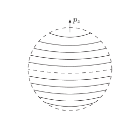
where and are the rest energy and cyclotron energy of electron, respectively. Here, is the momentum component along the field direction which is taken as the z-direction, , and are the Landau and spin quantum number, respectively. The density of states per unit volume for the energy level is given by , where is the density of states per unit area for a Landau energy level. As a consequence of quantization, the spherical Fermi surface of the free electron is replaced by a set of circles located on a spherical surface with a common axis along the direction, which is shown in Fig.2.
The susceptibility of the electron assembly can be obtained by finding its grand potential which depends on the density of states. It is a function of energy and magnetic induction. The density of states per unit volume is given by
| (5) |
where is the kinetic energy of an electron. The grand potential per unit volume of the assembly is given by
where , is the chemical potential, and is the Fermi-Dirac distribution function. After summing over the spin quantum number, Eq.(5) reduces to
| (6) |
where
| (7) |
and is the integer of (). For a neutron star, the electron system is almost completely degenerate () and the Fermi-Dirac distribution function is almost a step function except the region near . The magnetic moment depends on the first-order derivative of the grand potential with , and it mainly comes from the first-order derivative of Eq.(6) at Hence, we define . If the chemical potential of the neutron star is 10 MeV and the magnetic field is the quantum field G (the cyclotron energy of electron equals to its rest energy), then is about 200. Based on Eq.(7), we can see that the first-order derivative of the grand potential has a singularity when . Therefore, the susceptibility of the relativistic degenerate electron gas can be equal to or even larger than 1.
To reveal the oscillating effect of the grand potential, we calculate the sum of Eq.(7) with the Poisson summation formula (Dingle, 1952):
| (8) |
Because is much larger than 1, the density of states in Eq.(5) is approximately by
where denotes the Bernoulli numbers. The first two terms
on the right-hand side of the above equation are the non-oscillating parts while the third
term is the oscillating
part.
The non-oscillating grand potential per unit volume can be obtained from Eq.(10). As the first-order approximation, we can keep only the first term in the summation and obtain
In general, for a neutron star. Using the standard methods of evaluating integrals for the Fermi-Dirac distribution, we can evaluate the integrals in Eq.(11). The non-oscillating susceptibility is given by
In our work, the chemical potential and the magnetic field in the
deep crust of a normal neutron star are, respectively, about 10 MeV and G,
while the non-oscillating susceptibility can be
.
Using the approximate formula for the Fermi-Dirac distribution
| (9) |
and the Fresnel Integral
we obtain the oscillating term of the grand potential per unit volume,
where . When calculating the differential susceptibility which is the second derivative of Eq.(15), we only kept the most rapidly varying terms, that is, only differentiating cosines and sinusoidal. Because for a neutron star, the last term in Eq.(15) is dominant. The oscillating susceptibility is approximately given by
| (10) |
where
| (11) |
and
| (12) |
Here, in Eq.(17) is the fine structure constant. The result of Eq.(16) is similar to the result obtained in Visvanathan (1962). It indicates that the susceptibility oscillates with . We replace by . When we have . Note that the first term is a constant, thus the oscillation is a period function of . The differences of the magnetic induction in an oscillating period are the periods of , which are given by
| (13) |
The coefficients of the cosine functions in Eq.(16) include two terms. The first term is the result of complete degeneracy, while the second term comes from the thermal fluctuation and is proportional to the second power of temperature. For a typical neutron star, the chemical potential, magnetic field and temperature are of the order of 10 MeV, G, and K, respectively. The second term can be ignored because of . The oscillating susceptibility, , is mainly determined by . Fig.3 shows the relation between and . Obviously, the differential susceptibility can equal or exceed 1 when . In this work, we assume that the magnetars are similar to the normal neutron stars except their magnetic fields: for a normal neutron star, G, while for a magnetar . For a stronger magnetic field, the condition or cannot be satisfied, and the above approximate methods cannot be used. We will discuss them in the next paper.

4 The observed evidences in magnetars
As mentioned in the last section, the susceptibility of a relativistic degenerate electron gas can be equal to or exceed 1. The electron gas under a strong magnetic field in a neutron star may be in a unstable state, and the first-order phase transition should occur. Finally, the electron gas should be a stable state and has the Condon domain structure. The magnetizations in the adjacent domains have opposite directions.
Based on Eq.(19), the relative variation of the magnetic induction between adjacent magnetic domains is
| (14) |
For a normal neutron star ( G), , it is very difficult to observe the oscillatory effects. However, for magnetars (), , which is large enough to produce the bursts in SGRs or AXPs.
The adjacent magnetic domains have different electron densities. The different magnetizations in the adjacent magnetic domains mean that the phase difference is . According to Eq.(16), we have . For simplicity we approximate the chemical potential with the zero-temperature free field Fermi energy . The difference of electron densities between the adjacent magnetic domains is given by
| (15) |
where and we have taken . For a magnetar, MeV, , and the rest energy of electrons MeV. Obviously, here is scaled to 20 and to , respectively.
The electrons in a neutron star coexist with other components such as the nuclei in the crust or the Fermi liquid of protons and neutrons closed to the deep crust. Due to the Coulomb interactions among electrons, nuclei or protons, the matter of the neutron star may not be homogeneous, once the domain structure appears in the crust. However, it can not occur in the Fermi liquid. The mechanism of forming electron domains is the interactions among orbital magnetic moments which are counterbalanced by the degenerate pressure of electrons . Because the Coulomb interaction of the crystal lattices in the crust is the same order of magnitude with the interaction among the orbital magnetic moments, the electron domain structure can lead to the formation of the nuclei domain structure. However, in the Fermi liquid of nucleons, the neutron degenerate pressure , where is the fraction of electrons per neutron and it is only several tenths. The interaction among the orbital magnetic moments can not counterbalance the neutron degenerate pressure . Therefore, the magnetic domain structure cannot form in a Fermi liquid of nucleons. The magnetic system is in a metastable state, which is similar to the supercooling or superheating states in the first-order phase transition.
In the crust of a magnetar we can roughly calculate the size of the domain structure. With the density increasing, the quantum number of the Landau energy also increases. Using the gravitational potential energy of a nucleon and the Fermi energy per electron, we can estimate the height of the magnetic domains as (Suh & Mathews, 2010)
| (16) |
where is the surface gravity and is scaled to 0.36 when neutrons drip out from nuclei. The actual size and shape of the domains is problematical. There seem to be two possibilities (Blandford & Hernquist, 1982). The first is that the domains have a horizontal scale which is in general required if there is to be a balance in the electron pressures. The second possibility is that the domains form a two-dimensional lattice of vertical needles with a thickness given roughly by the geometrical mean of the cyclonic radius. This second configuration minimizes the magnetic and surface energies. If we assume that the volume change of the electron gas during forming the second domain configuration is only along the horizontal direction and the changing magnitude (or the thickness of domain walls) is a cyclonic radius of an electron, based on Eq.(21), the width of the magnetic domain for the second possibility can be estimated as
| (17) |
The Maxwell shearing stress between the adjacent domains can deform the crust and gives rise to a strain, . It is given by
| (18) |
where is the shear modulus of the crust and . Closed to the bottom of the crust, G (Baym & Pines, 1971). For magnetars, , according to Eqs.(20) and (24), we have the strain . Ruderman (1991) found that the maximum strain of the crust, , is . Our result clearly is within the range. When the domain structures appear in the crust of a magnetar, the shearing stress acting on adjacent domains can produce a relative shift or a fracture between them. This sudden shift or fracture can propagate with the Alfvén velocity along the domain layers, which results in a series of shifts or fractures in the magnetic domains. The time scale of shifts propagating along a domain layer is estimated as
| (19) |
where and are the Alfvén velocity (Duncan, 2004) and the matter density at the deep crust, respectively, is the length of the domain layer, and () the radius of the magnetar. The time scale agrees with the observed duration of the SGRs bursts (Thompson & Duncan, 1995). Available free energy equals the change of magnetic energy from a domain structure to a homogeneous structure. The density of magnetic free energy is
| (20) |
Then, the total free energy approximates to
| (21) |
According to Eq.(20) and Eq.(22), the total free energy is
| (22) |
where we scaled to cm and to
G when (See
Eq.(20)). This energy also agrees with the observations of bursts.
The Fermi liquid of nucleons in a magnetar may be in metastable state. A series of shifts in the deep crust closed to the Fermi liquid of nucleons can trigger the phase transition of the Fermi liquid of nucleons from a metastable state to a stable state. The free magnetic energy in the Fermi liquid is released and it is far greater than that in the crust because the magnetic induction and the thickness of the Fermi liquid is larger than the crust. The actual size of the fermi liquid of nucleons in metastable state is also problematical because of the unknowing configuration of electrons and magnetic field distributions. However, all the Fermi liquid of nucleons may evolve into metastable state simultaneously when the deep crust is stable. Let the magnetic induction of the Fermi liquid be at the same order of magnitude as that in the deep crust, and the thickness of the Fermi liquid be approximated by the radius of the magnetar. We estimate that the energy released is
| (23) |
This energy agrees with those released in the GFs of some magnetars.
5 Summary
We discussed the magnetization effects of the relativistic degenerate electron gas in a neutron star. Having considered the magnetic interaction among electrons, we found that the magnetic systems may be unstable or metastable when the differential susceptibility equals or exceeds 1. Under an ultra-strong magnetic field, the magnetic domain structures in a magnetar can appear in the solid crust, while the Fermi liquid of nucleons may be in metastable state. The shearing stress acting on adjacent domains can result in a series of shifts or fractures in the crust. The crust releases the magnetic free energy, which corresponds to the bursts observed in magnetars. Simultaneously, a series of shifts or fractures in the deep crust closed to the Fermi liquid of nucleons can trigger the phase transition of the Fermi liquid from a metastable state to a stable state. The free magnetic energy in the Fermi liquid of nucleons is released, which corresponds to the GFs observed in some magnetars.
Acknowledgments
We thank the anonymous referee for his/ her comments which helped to improve the paper. ZJ thanks Prof. Anzhong Wang for correcting the English language of the manuscript. This work was supported in part by the National Science Foundation of China (Grants Nos. 10963003, 11063002 and 11163005), Foundation of Huoyingdong under No. 121107, Foundation of Ministry of Education under No. 211198 and the Doctor Foundation of Xinjiang University (Grant No.BS110108).
References
- Baym & Pines (1971) Baym, G., & Pines, D. 1971, Annals of Physics, 66, 816
- Blandford & Hernquist (1982) Blandford, R. D., & Hernquist, L. 1982, Journal of Physics C Solid State Physics, 15, 6233
- Canuto & Chiu (1968) Canuto, V., & Chiu, H.-Y. 1968, Physical Review, 173, 1229
- Chudnovsky (1981) Chudnovsky, E. M. 1981, Journal of Physics A Mathematical General, 14, 2091
- Cline et al. (1982) Cline, T. L., et al. 1982, ApJL, 255, L45
- Condon (1966) Condon, J. H. 1966, Physical Review, 145, 526
- Dingle (1952) Dingle, R. B. 1952, Royal Society of London Proceedings Series A, 211, 500
- Duncan (2004) Duncan, R. C. 2004, in Cosmic explosions in three dimensions, ed. P. Höflich, P. Kumar, & J. C. Wheeler, 285
- Duncan & Thompson (1992) Duncan, R. C., & Thompson, C. 1992, ApJ, 392, L9
- Goldreich & Reisenegger (1992) Goldreich, P., & Reisenegger, A. 1992, ApJ, 395, 250
- Hurley et al. (1999) Hurley, K., et al. 1999, Nature, 397, 41
- Johnson & Lippmann (1949) Johnson, M. H., & Lippmann, B. A. 1949, Physical Review, 76, 828
- Kondratyev (2002) Kondratyev, V. N. 2002, Physical Review Letters, 88, 221101
- Lee et al. (1969) Lee, H. J., Canuto, V., Chiu, H.-Y., & Chiuderi, C. 1969, Physical Review Letters, 23, 390
- Lifshits & Kosevich (1956) Lifshits, E. M., & Kosevich, A. M. 1956, Sov.Phys.-JETP, 2, 636
- Mazets et al. (1999) Mazets, E. P., Cline, T. L., Aptekar’, R. L., Butterworth, P. S., Frederiks, D. D., Golenetskii, S. V., Il’Inskii, V. N., & Pal’Shin, V. D. 1999, Astronomy Letters, 25, 635
- Mazets et al. (1979) Mazets, E. P., Golentskii, S. V., Ilinskii, V. N., Aptekar, R. L., & Guryan, I. A. 1979, Nature, 282, 587
- O’Connell & Roussel (1971) O’Connell, R. F., & Roussel, K. M. 1971, Nature, 231, 32
- Palmer et al. (2005) Palmer, D. M., et al. 2005, Nature, 434, 1107
- Pippard (1963) Pippard, A. B. 1963, Royal Society of London Proceedings Series A, 272, 192
- Pippard (1980) —. 1980, in Electrons at the Fermi surface, ed M. Springford (Cambridge: Cambridge University press)
- Reichl (1998) Reichl, L. E. 1998, A Modern Course in Statistical Physics, 2nd Edition
- Ruderman (1991) Ruderman, R. 1991, ApJ, 382, 576
- Shoenberg (1962) Shoenberg, D. 1962, Royal Society of London Philosophical Transactions Series A, 255, 85
- Shoenberg (1984) —. 1984, Magnetic oscillation in metals(Cambridge: Cambridge University press)
- Stella et al. (2005) Stella, L., Dall’Osso, S., Israel, G. L., & Vecchio, A. 2005, ApJ, 634, L165
- Suh & Mathews (2010) Suh, I.-S., & Mathews, G. J. 2010, ApJ, 717, 843
- Terasawa et al. (2005) Terasawa, T., et al. 2005, Nature, 434, 1110
- Thompson & Duncan (1995) Thompson, C., & Duncan, R. C. 1995, MNRAS, 275, 255
- Thompson & Duncan (2001) —. 2001, ApJ, 561, 980
- Visvanathan (1962) Visvanathan, S. 1962, Physics of Fluids, 5, 701
- Wilkes & Ingraham (1989) Wilkes, J. M., & Ingraham, R. L. 1989, ApJ, 344, 399