State estimation under non-Gaussian Lévy noise:
A modified Kalman filtering method 111This work was partly supported by the NSF grant DMS-1025422.

Xu Sun1,2, Jinqiao Duan2,3, Xiaofan Li2 and Xiangjun Wang1
1. Huazhong University of Science and Technology
Wuhan 430074, Hubei, China
E-mail: xjwang@hust.edu.cn
2. Illinois Institute of Technology
Chicago, IL 60616, USA
E-mail: lix@iit.edu
3. Institute for Pure and Applied Mathematics
University of California
Los Angeles, CA 90095, USA
E-mail: jduan@ipam.ucla.edu
Abstract

The Kalman filter is extensively used for state estimation for linear systems under Gaussian noise. When non-Gaussian Lévy noise is present, the conventional Kalman filter may fail to be effective due to the fact that the non-Gaussian Lévy noise may have infinite variance. A modified Kalman filter for linear systems with non-Gaussian Lévy noise is devised. It works effectively with reasonable computational cost. Simulation results are presented to illustrate this non-Gaussian filtering method.

Keywords: Kalman filter, modified Kalman filter, Non-Gaussian noise, Lévy noise, state estimation, data assimilation

1 Introduction and statement of the problem

The Kalman filter, or the Kalman filtering method, provides an efficient way to estimate the state of a linear dynamical system subject to Gaussian white noise [5, 6, 7]. It has been widely used in applications such as target tracking, parameter estimation, control theory, signal processing, and other data assimilation tasks.

The Kalman filter requires the noise be either Gaussian or with finite variance [5, 6], and thus it is not applicable to linear systems with non-Gaussian noise of infinite variance. As non-Gaussian Lévy noise with infinite variance exists ubiquitously [10, 9], it is desirable to study the Kalman filtering problems under Lévy noise. Very little work has been done for this issue. Breton and Musiela [4] presented a scheme for Kalman filtering with noise of infinite variance, while assuming the contribution of the jumps are exactly known. The filter in [4] is nonlinear and recursive, and thus may greatly limit its application in practice. Ahn and Feldman [1] proposed to minimize the difference between the true state and the filtered observation in the Lμsuperscript𝐿𝜇L^{\mu}-norm. However, as pointed in [9], this method does not really address the Kalman filtering problem which consists of combining forecasts and observations. The method in [9] focuses on large errors and has a robust performance but high computational cost due to the matrix diagonalization and the operation of the fractional power in each step. This may also be an obstacle for real-time implementation in practical applications. Note that in practice, each iteration step must be completed during every sampling period, and it is greatly desirable to make the algorithm as fast as possible.

In this paper, we will present an algorithm, which has the similar computational cost as that of the Kalman filter, but can be applied to linear systems with non-Gaussian Lévy noise of infinite variance.

We consider the following discrete time model with the state equation

𝐱k+1=𝐅k𝐱k+𝐰k,subscript𝐱𝑘1subscript𝐅𝑘subscript𝐱𝑘subscript𝐰𝑘\displaystyle\mathbf{x}_{k+1}=\mathbf{F}_{k}\mathbf{x}_{k}+\mathbf{w}_{k}, (1)

and the observation equation

𝐳k=𝐇k𝐱k+𝐯k,subscript𝐳𝑘subscript𝐇𝑘subscript𝐱𝑘subscript𝐯𝑘\displaystyle\mathbf{z}_{k}=\mathbf{H}_{k}\mathbf{x}_{k}+\mathbf{v}_{k}, (2)

where 𝐱ksubscript𝐱𝑘\mathbf{x}_{k}, an n𝑛n-by-111 vector, is the state variable, and 𝐳ksubscript𝐳𝑘\mathbf{z}_{k}, an m𝑚m-by-111 vector, is the measurement (or observation) variable, 𝐰ksubscript𝐰𝑘\mathbf{w}_{k} represents the modeling error noise, 𝐯ksubscript𝐯𝑘\mathbf{v}_{k} the measurement error noise, and 𝐅ksubscript𝐅𝑘\mathbf{F}_{k} and 𝐇ksubscript𝐇𝑘\mathbf{H}_{k} are n𝑛n-by-n𝑛n and m𝑚m-by-n𝑛n matrices, respectively. We only consider the cases where 𝐰ksubscript𝐰𝑘\mathbf{w}_{k} is a Gaussian noise, and 𝐯ksubscript𝐯𝑘\mathbf{v}_{k} is a non-Gaussian Lévy noise.

This paper is arranged as follows. In section 2, the usual Kalman filter is briefly reviewed. The proposed modified Kalman filter is presented in section 3. A simulation example is provided in Section 4 to illustrate the effectiveness of the modified Kalman filter.

2 Review of the conventional Kalman filter

A derivation of the Kalman filter is briefly reviewed in this section. Some equations and ideas presented in this section will be used to present our proposed modified Kalman filter in the next section. Derivations of the Kalman filter can be found in many references [5, 6, 7].

Consider the model as given in (1) and (2). The Kalman filtering assumes that both the modeling error noise 𝐰ksubscript𝐰𝑘\mathbf{w}_{k} and the measurement disturbance 𝐯ksubscript𝐯𝑘\mathbf{v}_{k} are Gaussian with the following covariance matrix,

E[𝐰i𝐰kT]={𝐐k,fori=k,0,forik.𝐸delimited-[]subscript𝐰𝑖superscriptsubscript𝐰𝑘𝑇casessubscript𝐐𝑘for𝑖𝑘0for𝑖𝑘\displaystyle E\left[\mathbf{w}_{i}\mathbf{w}_{k}^{T}\right]=\begin{cases}\mathbf{Q}_{k},&\text{for}\quad i=k,\\ 0,&\text{for}\quad i\neq k.\\ \end{cases} (3)
E[𝐯i𝐯kT]={𝐑k,fori=k,0,forik.𝐸delimited-[]subscript𝐯𝑖superscriptsubscript𝐯𝑘𝑇casessubscript𝐑𝑘for𝑖𝑘0for𝑖𝑘\displaystyle E\left[\mathbf{v}_{i}\mathbf{v}_{k}^{T}\right]=\begin{cases}\mathbf{R}_{k},&\text{for}\quad i=k,\\ 0,&\text{for}\quad i\neq k.\\ \end{cases} (4)

Let 𝐱¯ksubscript¯𝐱𝑘\bar{\mathbf{x}}_{k} be the priori estimate, which is the estimate of 𝐱ksubscript𝐱𝑘\mathbf{x}_{k} given 𝐳0subscript𝐳0\mathbf{z}_{0}, 𝐳1subscript𝐳1\mathbf{z}_{1}, \cdots, 𝐳k1subscript𝐳𝑘1\mathbf{z}_{k-1}, and let 𝐱^ksubscript^𝐱𝑘\hat{\mathbf{x}}_{k} be the posterior estimate, which is the estimate of 𝐱ksubscript𝐱𝑘\mathbf{x}_{k} given 𝐳0subscript𝐳0\mathbf{z}_{0}, 𝐳1subscript𝐳1\mathbf{z}_{1}, \cdots, 𝐳ksubscript𝐳𝑘\mathbf{z}_{k}. It is known that

E{𝐱¯k}=E{𝐱k}𝐸subscript¯𝐱𝑘𝐸subscript𝐱𝑘\displaystyle E\{\bar{\mathbf{x}}_{k}\}=E\{\mathbf{x}_{k}\} (5)

and

𝐱¯k+1=𝐅k𝐱^k,subscript¯𝐱𝑘1subscript𝐅𝑘subscript^𝐱𝑘\displaystyle\bar{\mathbf{x}}_{k+1}=\mathbf{F}_{k}\hat{\mathbf{x}}_{k}, (6)

where E{}𝐸E\{\cdot\} represents expectation and 𝐅ksubscript𝐅𝑘\mathbf{F}_{k} is from (1).

The Kalman filter assumes that the posterior estimate is expressed as the prior estimate corrected by the measurement data,

𝐱^k=𝐱¯k+𝐊k(𝐳k𝐇k𝐱¯k),subscript^𝐱𝑘subscript¯𝐱𝑘subscript𝐊𝑘subscript𝐳𝑘subscript𝐇𝑘subscript¯𝐱𝑘\displaystyle\hat{\mathbf{x}}_{k}=\bar{\mathbf{x}}_{k}+\mathbf{K}_{k}\left(\mathbf{z}_{k}-\mathbf{H}_{k}\bar{\mathbf{x}}_{k}\right), (7)

for some n𝑛n-by-m𝑚m matrix 𝐊ksubscript𝐊𝑘\mathbf{K}_{k} (so called Kalman gain). Note that 𝐇ksubscript𝐇𝑘\mathbf{H}_{k} is from (2). The Kalman gain 𝐊ksubscript𝐊𝑘\mathbf{K}_{k} is solved by minimizing E[(𝐱^k𝐱k)2]𝐸delimited-[]superscriptsubscript^𝐱𝑘subscript𝐱𝑘2E\left[(\hat{\mathbf{x}}_{k}-\mathbf{x}_{k})^{2}\right]. Note that

E[(𝐱^k𝐱k)T(𝐱^k𝐱k)]=Tr{𝐏k},𝐸delimited-[]superscriptsubscript^𝐱𝑘subscript𝐱𝑘𝑇subscript^𝐱𝑘subscript𝐱𝑘Trsubscript𝐏𝑘\displaystyle E\left[(\hat{\mathbf{x}}_{k}-\mathbf{x}_{k})^{T}(\hat{\mathbf{x}}_{k}-\mathbf{x}_{k})\right]=\text{Tr}\{\mathbf{P}_{k}\}, (8)

where Tr{}Tr\text{Tr}\{\cdot\} represents the trace operator, and the n𝑛n-by-n𝑛n covariance matrix 𝐏ksubscript𝐏𝑘\mathbf{P}_{k} is defined as follows

𝐏k=E[(𝐱k𝐱^k)(𝐱k𝐱^k)T].subscript𝐏𝑘𝐸delimited-[]subscript𝐱𝑘subscript^𝐱𝑘superscriptsubscript𝐱𝑘subscript^𝐱𝑘𝑇\displaystyle\mathbf{P}_{k}=E\left[(\mathbf{x}_{k}-\hat{\mathbf{x}}_{k})(\mathbf{x}_{k}-\hat{\mathbf{x}}_{k})^{T}\right]. (9)

Define

𝐏¯k=E[(𝐱k𝐱¯k)(𝐱k𝐱¯k)T].subscript¯𝐏𝑘𝐸delimited-[]subscript𝐱𝑘subscript¯𝐱𝑘superscriptsubscript𝐱𝑘subscript¯𝐱𝑘𝑇\displaystyle\bar{\mathbf{P}}_{k}=E\left[(\mathbf{x}_{k}-\bar{\mathbf{x}}_{k})(\mathbf{x}_{k}-\bar{\mathbf{x}}_{k})^{T}\right]. (10)

It follows from (3), (4), (9) and (10) that

𝐏¯k+1=𝐅k𝐏k𝐅kT+𝐐k.subscript¯𝐏𝑘1subscript𝐅𝑘subscript𝐏𝑘superscriptsubscript𝐅𝑘𝑇subscript𝐐𝑘\displaystyle\bar{\mathbf{P}}_{k+1}=\mathbf{F}_{k}\mathbf{P}_{k}\mathbf{F}_{k}^{T}+\mathbf{Q}_{k}. (11)

Substituting (7) into (9), we get

𝐏k=(𝐈𝐊k𝐇k)𝐏¯k(𝐈𝐊k𝐇k)T+𝐊k𝐑k𝐊kT.subscript𝐏𝑘𝐈subscript𝐊𝑘subscript𝐇𝑘subscript¯𝐏𝑘superscript𝐈subscript𝐊𝑘subscript𝐇𝑘𝑇subscript𝐊𝑘subscript𝐑𝑘superscriptsubscript𝐊𝑘𝑇\displaystyle\mathbf{P}_{k}=(\mathbf{I}-\mathbf{K}_{k}\mathbf{H}_{k})\bar{\mathbf{P}}_{k}(\mathbf{I}-\mathbf{K}_{k}\mathbf{H}_{k})^{T}+\mathbf{K}_{k}\mathbf{R}_{k}\mathbf{K}_{k}^{T}. (12)

It follows from (12) that

dd𝐊kTr{𝐏k}=2(𝐇K𝐏¯k)T+2𝐊k(𝐇k𝐏¯k𝐇kT+𝐑k).𝑑𝑑subscript𝐊𝑘𝑇𝑟subscript𝐏𝑘2superscript𝐇𝐾subscript¯𝐏𝑘𝑇2subscript𝐊𝑘subscript𝐇𝑘subscript¯𝐏𝑘superscriptsubscript𝐇𝑘𝑇subscript𝐑𝑘\displaystyle\frac{d}{d\mathbf{K}_{k}}Tr\{\mathbf{P}_{k}\}=-2(\mathbf{H}-K\bar{\mathbf{P}}_{k})^{T}+2\mathbf{K}_{k}(\mathbf{H}_{k}\bar{\mathbf{P}}_{k}\mathbf{H}_{k}^{T}+\mathbf{R}_{k}). (13)

Solve 𝐊ksubscript𝐊𝑘\mathbf{K}_{k} by letting dd𝐊kTr{𝐏k}=0𝑑𝑑subscript𝐊𝑘𝑇𝑟subscript𝐏𝑘0\frac{d}{d\mathbf{K}_{k}}Tr\{\mathbf{P}_{k}\}=0, we get

𝐊k=𝐏¯k𝐇kT(𝐇k𝐏¯k𝐇kT+𝐑k)1subscript𝐊𝑘subscript¯𝐏𝑘superscriptsubscript𝐇𝑘𝑇superscriptsubscript𝐇𝑘subscript¯𝐏𝑘superscriptsubscript𝐇𝑘𝑇subscript𝐑𝑘1\displaystyle\mathbf{K}_{k}=\bar{\mathbf{P}}_{k}\mathbf{H}_{k}^{T}(\mathbf{H}_{k}\bar{\mathbf{P}}_{k}\mathbf{H}_{k}^{T}+\mathbf{R}_{k})^{-1} (14)

By (12) and (14), 𝐏ksubscript𝐏𝑘\mathbf{P}_{k} can be rewritten as

𝐏k=(𝐈𝐊k𝐇k)𝐏¯k.subscript𝐏𝑘𝐈subscript𝐊𝑘subscript𝐇𝑘subscript¯𝐏𝑘\displaystyle\mathbf{P}_{k}=(\mathbf{I}-\mathbf{K}_{k}\mathbf{H}_{k})\bar{\mathbf{P}}_{k}. (15)

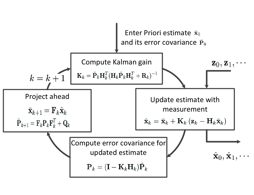
Combining (6), (14) and (15), we thus have the conventional Kalman filter. This algorithm is shown in Figure 1.

3 A modified Kalman filter

It is known that the discrete time Gaussian white noise can be approximated by the increments of Brownian motion per time step, and the non-Gaussian Lévy noise can be approximated by the increments of the corresponding Lévy process per time step. By Lévy-Ito theorem [2], a Lévy process can be decomposed into the sum of a Gaussian process and a pure jump process. It is shown in [3] that the small jumps of a Lévy process can be approximated by a Gaussian process. Therefore, we can approximately regard a Lévy process as combination of a Gaussian process and a process with big jumps. For more information about decomposition of a Lévy processes, see [3, 2]. These results enable us to decompose a non-Gaussian Lévy noise into a Gaussian white noise plus some extremely large values.

In our proposed filtering method, we convert the original Lévy noise into a Gaussian white noise by clipping off its extremely large values.

Let 𝐯~ksubscript~𝐯𝑘\tilde{\mathbf{v}}_{k} represent the clipped version of the Lévy measurement disturbance 𝐯ksubscript𝐯𝑘\mathbf{v}_{k}, and let 𝐳~ksubscript~𝐳𝑘\tilde{\mathbf{z}}_{k} represent the corresponding clipped observation. Thus

𝐳~k=𝐇k𝐱k+𝐯~k.subscript~𝐳𝑘subscript𝐇𝑘subscript𝐱𝑘subscript~𝐯𝑘\displaystyle\tilde{\mathbf{z}}_{k}=\mathbf{H}_{k}\mathbf{x}_{k}+\tilde{\mathbf{v}}_{k}. (16)

In practice, since the measurement noise, 𝐯ksubscript𝐯𝑘\mathbf{v}_{k}, is unknown, we propose to clip the observation 𝐳ksubscript𝐳𝑘\mathbf{z}_{k} instead of 𝐯ksubscript𝐯𝑘\mathbf{v}_{k} in a component-wise way by the following operation:

𝐳~ki={j𝐇ki,j𝐱¯kj+Csign(𝐳kij𝐇ki,j𝐱¯kj)if|𝐳kij𝐇ki,j𝐱¯kj|C,𝐳kiif|𝐳kij𝐇ki,j𝐱¯kj|<C,superscriptsubscript~𝐳𝑘𝑖casessubscript𝑗superscriptsubscript𝐇𝑘𝑖𝑗superscriptsubscript¯𝐱𝑘𝑗𝐶signsuperscriptsubscript𝐳𝑘𝑖subscript𝑗superscriptsubscript𝐇𝑘𝑖𝑗superscriptsubscript¯𝐱𝑘𝑗ifsuperscriptsubscript𝐳𝑘𝑖subscript𝑗superscriptsubscript𝐇𝑘𝑖𝑗superscriptsubscript¯𝐱𝑘𝑗𝐶superscriptsubscript𝐳𝑘𝑖ifsuperscriptsubscript𝐳𝑘𝑖subscript𝑗superscriptsubscript𝐇𝑘𝑖𝑗superscriptsubscript¯𝐱𝑘𝑗𝐶\displaystyle\tilde{\mathbf{z}}_{k}^{i}=\begin{cases}\sum_{j}\mathbf{H}_{k}^{i,j}\bar{\mathbf{x}}_{k}^{j}+C\cdot\text{sign}\left(\mathbf{z}_{k}^{i}-\sum_{j}\mathbf{H}_{k}^{i,j}\bar{\mathbf{x}}_{k}^{j}\right)&\text{if}\quad|\mathbf{z}_{k}^{i}-\sum_{j}\mathbf{H}_{k}^{i,j}\bar{\mathbf{x}}_{k}^{j}|\geq C,\\ \mathbf{z}_{k}^{i}&\text{if}\quad|\mathbf{z}_{k}^{i}-\sum_{j}\mathbf{H}_{k}^{i,j}\bar{\mathbf{x}}_{k}^{j}|<C,\\ \end{cases} (17)

where C𝐶C is some positive threshold value, 𝐳kisuperscriptsubscript𝐳𝑘𝑖\mathbf{z}_{k}^{i} and 𝐱¯kisuperscriptsubscript¯𝐱𝑘𝑖\bar{\mathbf{x}}_{k}^{i} represent the i𝑖i-th components of the vectors 𝐳ksubscript𝐳𝑘\mathbf{z}_{k} and 𝐱¯ksubscript¯𝐱𝑘\bar{\mathbf{x}}_{k}, respectively, and j𝐇ki,j𝐱¯kjsubscript𝑗superscriptsubscript𝐇𝑘𝑖𝑗superscriptsubscript¯𝐱𝑘𝑗\sum_{j}\mathbf{H}_{k}^{i,j}\bar{\mathbf{x}}_{k}^{j} is the i𝑖i-th component of the vector 𝐇k𝐱¯ksubscript𝐇𝑘subscript¯𝐱𝑘\mathbf{H}_{k}\bar{\mathbf{x}}_{k}. Note that C𝐶C is determined by the statistical properties of the measurement noise 𝐯ksubscript𝐯𝑘\mathbf{v}_{k}. Replacing the observation value 𝐳ksubscript𝐳𝑘\mathbf{z}_{k} in (7) with its clipped value, we get

𝐱^k=𝐱¯k+𝐊k(𝐳~k𝐇k𝐱¯k).subscript^𝐱𝑘subscript¯𝐱𝑘subscript𝐊𝑘subscript~𝐳𝑘subscript𝐇𝑘subscript¯𝐱𝑘\displaystyle\hat{\mathbf{x}}_{k}=\bar{\mathbf{x}}_{k}+\mathbf{K}_{k}\left(\tilde{\mathbf{z}}_{k}-\mathbf{H}_{k}\bar{\mathbf{x}}_{k}\right). (18)

Repeating the same procedure in Section 222 to solve the Kalman gain 𝐊ksubscript𝐊𝑘\mathbf{K}_{k} by minimizing E{(𝐱k𝐱^k)2}𝐸superscriptsubscript𝐱𝑘subscript^𝐱𝑘2E\{(\mathbf{x}_{k}-\hat{\mathbf{x}}_{k})^{2}\}, we get

𝐊k=𝐏¯k𝐇kT(𝐇k𝐏¯k𝐇kT+𝐑~k)1,subscript𝐊𝑘subscript¯𝐏𝑘superscriptsubscript𝐇𝑘𝑇superscriptsubscript𝐇𝑘subscript¯𝐏𝑘superscriptsubscript𝐇𝑘𝑇subscript~𝐑𝑘1\displaystyle\mathbf{K}_{k}=\bar{\mathbf{P}}_{k}\mathbf{H}_{k}^{T}(\mathbf{H}_{k}\bar{\mathbf{P}}_{k}\mathbf{H}_{k}^{T}+\tilde{\mathbf{R}}_{k})^{-1}, (19)

where 𝐑~ksubscript~𝐑𝑘\tilde{\mathbf{R}}_{k} is the covariance matrix of 𝐯~ksubscript~𝐯𝑘\tilde{\mathbf{v}}_{k} defined as

𝐑~k=E{𝐯~k𝐯~kT}.subscript~𝐑𝑘𝐸subscript~𝐯𝑘superscriptsubscript~𝐯𝑘𝑇\displaystyle\tilde{\mathbf{R}}_{k}=E\left\{\tilde{\mathbf{v}}_{k}\tilde{\mathbf{v}}_{k}^{T}\right\}. (20)

In the conventional Kalman filter, 𝐐ksubscript𝐐𝑘\mathbf{Q}_{k} and 𝐑ksubscript𝐑𝑘\mathbf{R}_{k} are assumed to be known, and as noted in [6], it is often a difficult task to estimate the covariance matrices 𝐐ksubscript𝐐𝑘\mathbf{Q}_{k} and 𝐑ksubscript𝐑𝑘\mathbf{R}_{k}.

In the modified Kalman filter here, we only assume 𝐐ksubscript𝐐𝑘\mathbf{Q}_{k} is known and suggest 𝐑~ksubscript~𝐑𝑘\tilde{\mathbf{R}}_{k} be estimated as follows. It follows from (16) and (17) that

𝐑~k=subscript~𝐑𝑘absent\displaystyle\tilde{\mathbf{R}}_{k}= E{𝐯~k𝐯~kT}𝐸subscript~𝐯𝑘superscriptsubscript~𝐯𝑘𝑇\displaystyle E\left\{\tilde{\mathbf{v}}_{k}\tilde{\mathbf{v}}_{k}^{T}\right\}
=\displaystyle= E{[(𝐳~k𝐇k𝐱¯k)𝐇k(𝐱k𝐱¯k)][(𝐳~k𝐇k𝐱¯k)𝐇k(𝐱k𝐱¯k)]T}𝐸delimited-[]subscript~𝐳𝑘subscript𝐇𝑘subscript¯𝐱𝑘subscript𝐇𝑘subscript𝐱𝑘subscript¯𝐱𝑘superscriptdelimited-[]subscript~𝐳𝑘subscript𝐇𝑘subscript¯𝐱𝑘subscript𝐇𝑘subscript𝐱𝑘subscript¯𝐱𝑘𝑇\displaystyle E\left\{\left[(\tilde{\mathbf{z}}_{k}-\mathbf{H}_{k}\bar{\mathbf{x}}_{k})-\mathbf{H}_{k}(\mathbf{x}_{k}-\bar{\mathbf{x}}_{k})\right]\left[(\tilde{\mathbf{z}}_{k}-\mathbf{H}_{k}\bar{\mathbf{x}}_{k})-\mathbf{H}_{k}(\mathbf{x}_{k}-\bar{\mathbf{x}}_{k})\right]^{T}\right\}
=\displaystyle= (𝐳~k𝐇k𝐱¯k)(𝐳~k𝐇k𝐱¯k)T+𝐇k𝐏¯k𝐇kT.subscript~𝐳𝑘subscript𝐇𝑘subscript¯𝐱𝑘superscriptsubscript~𝐳𝑘subscript𝐇𝑘subscript¯𝐱𝑘𝑇subscript𝐇𝑘subscript¯𝐏𝑘superscriptsubscript𝐇𝑘𝑇\displaystyle(\tilde{\mathbf{z}}_{k}-\mathbf{H}_{k}\bar{\mathbf{x}}_{k})(\tilde{\mathbf{z}}_{k}-\mathbf{H}_{k}\bar{\mathbf{x}}_{k})^{T}+\mathbf{H}_{k}\bar{\mathbf{P}}_{k}\mathbf{H}_{k}^{T}. (21)

In deriving the last identity of (3), we have used the fact that 𝐳~ksubscript~𝐳𝑘\tilde{\mathbf{z}}_{k} and 𝐱¯ksubscript¯𝐱𝑘\bar{\mathbf{x}}_{k} are known values and

E{(𝐳~k𝐇k𝐱¯k)(𝐱k𝐱¯k)T𝐇kT}=(𝐳~k𝐇k𝐱¯k)E{(𝐱k𝐱¯k)T}𝐇kT=0.𝐸subscript~𝐳𝑘subscript𝐇𝑘subscript¯𝐱𝑘superscriptsubscript𝐱𝑘subscript¯𝐱𝑘𝑇superscriptsubscript𝐇𝑘𝑇subscript~𝐳𝑘subscript𝐇𝑘subscript¯𝐱𝑘𝐸superscriptsubscript𝐱𝑘subscript¯𝐱𝑘𝑇superscriptsubscript𝐇𝑘𝑇0\displaystyle E\left\{(\tilde{\mathbf{z}}_{k}-\mathbf{H}_{k}\bar{\mathbf{x}}_{k})(\mathbf{x}_{k}-\bar{\mathbf{x}}_{k})^{T}\mathbf{H}_{k}^{T}\right\}=(\tilde{\mathbf{z}}_{k}-\mathbf{H}_{k}\bar{\mathbf{x}}_{k})E\{(\mathbf{x}_{k}-\bar{\mathbf{x}}_{k})^{T}\}\mathbf{H}_{k}^{T}=0. (22)

With (3), (19) can be rewritten as

𝐊k=𝐏¯k𝐇kT(2𝐇k𝐏¯k𝐇kT+𝐑~~k)1,subscript𝐊𝑘subscript¯𝐏𝑘superscriptsubscript𝐇𝑘𝑇superscript2subscript𝐇𝑘subscript¯𝐏𝑘superscriptsubscript𝐇𝑘𝑇subscript~~𝐑𝑘1\displaystyle\mathbf{K}_{k}=\bar{\mathbf{P}}_{k}\mathbf{H}_{k}^{T}(2\cdot\mathbf{H}_{k}\bar{\mathbf{P}}_{k}\mathbf{H}_{k}^{T}+\tilde{\tilde{\mathbf{R}}}_{k})^{-1}, (23)

where

𝐑~~k=(𝐳~k𝐇k𝐱¯k)(𝐳~k𝐇k𝐱¯k)T.subscript~~𝐑𝑘subscript~𝐳𝑘subscript𝐇𝑘subscript¯𝐱𝑘superscriptsubscript~𝐳𝑘subscript𝐇𝑘subscript¯𝐱𝑘𝑇\displaystyle\tilde{\tilde{\mathbf{R}}}_{k}=(\tilde{\mathbf{z}}_{k}-\mathbf{H}_{k}\bar{\mathbf{x}}_{k})(\tilde{\mathbf{z}}_{k}-\mathbf{H}_{k}\bar{\mathbf{x}}_{k})^{T}. (24)

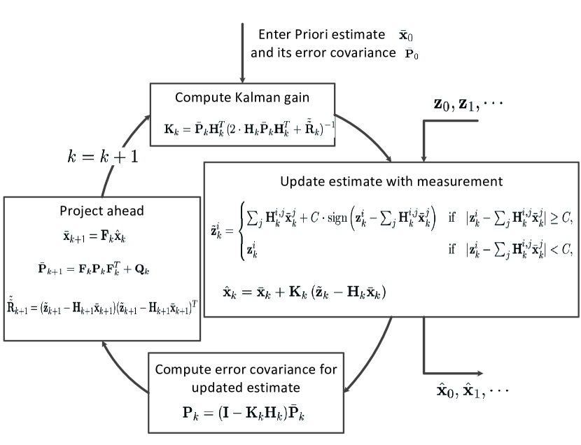
Combining equations (17), (18), (23), and (24), we obtain the modified Kalman filter, as shown graphically in Figure 2.

Comparing with the conventional Kalman filter, the proposed filter has an moderately increased computational cost due to the following two operations: i) the clipping operation for 𝐳ksubscript𝐳𝑘\mathbf{z}_{k}; ii) the computation of R~~ksubscript~~𝑅𝑘\tilde{\tilde{R}}_{k}. The former operation is implemented by IF-ElSE sentence, and the latter is simply a vector-vector outer product.

4 Simulation results

Consider a particle moving in the plane at some velocity subject to random perturbations in its trajectory. The new position at time k+1𝑘1k+1 is equal to the old position at time k𝑘k plus the velocity and noise. The model can be expressed in form of (1) and (2) as

(xk+11xk+12uk+11uk+12)=(1010010100100001)(xk1xk2uk1uk2)+(wk1wk2wk3wk4),matrixsubscriptsuperscript𝑥1𝑘1subscriptsuperscript𝑥2𝑘1subscriptsuperscript𝑢1𝑘1subscriptsuperscript𝑢2𝑘1matrixmissing-subexpression1010missing-subexpression0101missing-subexpression0010missing-subexpression0001matrixsubscriptsuperscript𝑥1𝑘subscriptsuperscript𝑥2𝑘subscriptsuperscript𝑢1𝑘subscriptsuperscript𝑢2𝑘matrixsubscriptsuperscript𝑤1𝑘subscriptsuperscript𝑤2𝑘subscriptsuperscript𝑤3𝑘subscriptsuperscript𝑤4𝑘\displaystyle\begin{pmatrix}x^{1}_{k+1}\\ x^{2}_{k+1}\\ u^{1}_{k+1}\\ u^{2}_{k+1}\end{pmatrix}=\begin{pmatrix}&1&0&1&0\\ &0&1&0&1\\ &0&0&1&0\\ &0&0&0&1\end{pmatrix}\begin{pmatrix}x^{1}_{k}\\ x^{2}_{k}\\ u^{1}_{k}\\ u^{2}_{k}\end{pmatrix}+\begin{pmatrix}w^{1}_{k}\\ w^{2}_{k}\\ w^{3}_{k}\\ w^{4}_{k}\end{pmatrix}, (25)

and

𝐳k=(10000100)𝐱k+(vk1vk2),subscript𝐳𝑘matrixmissing-subexpression1000missing-subexpression0100subscript𝐱𝑘matrixsubscriptsuperscript𝑣1𝑘subscriptsuperscript𝑣2𝑘\displaystyle\mathbf{z}_{k}=\begin{pmatrix}&1&0&0&0\\ &0&1&0&0\end{pmatrix}\mathbf{x}_{k}+\begin{pmatrix}v^{1}_{k}\\ v^{2}_{k}\end{pmatrix}, (26)

where (xk1subscriptsuperscript𝑥1𝑘x^{1}_{k}, xk2subscriptsuperscript𝑥2𝑘x^{2}_{k}) is the position at time k𝑘k, uk1subscriptsuperscript𝑢1𝑘u^{1}_{k}, uk2subscriptsuperscript𝑢2𝑘u^{2}_{k} the velocity, wk1subscriptsuperscript𝑤1𝑘w^{1}_{k}, wk2superscriptsubscript𝑤𝑘2w_{k}^{2}, wk3superscriptsubscript𝑤𝑘3w_{k}^{3}, and wk4superscriptsubscript𝑤𝑘4w_{k}^{4} are all Gaussian white noises with zero mean and unit variance, and vk1superscriptsubscript𝑣𝑘1v_{k}^{1} and vk2superscriptsubscript𝑣𝑘2v_{k}^{2} are independent and identically distributed noises consist of two components: i) a symmetric α𝛼\alpha-stable Lévy noises with the index of stability α=1.3𝛼1.3\alpha=1.3 and the scale parameter σ=10𝜎10\sigma=10 (see [8]); ii) a Gaussian white noise with variance of 5. Since the measurement noises, vk1superscriptsubscript𝑣𝑘1v_{k}^{1} and vk2superscriptsubscript𝑣𝑘2v_{k}^{2}, have infinite variances, the conventional Kalman filter can not be applied to estimate the position xk1superscriptsubscript𝑥𝑘1x_{k}^{1} and xk2superscriptsubscript𝑥𝑘2x_{k}^{2}. So we apply the modified Kalman filter proposed in the previous section.

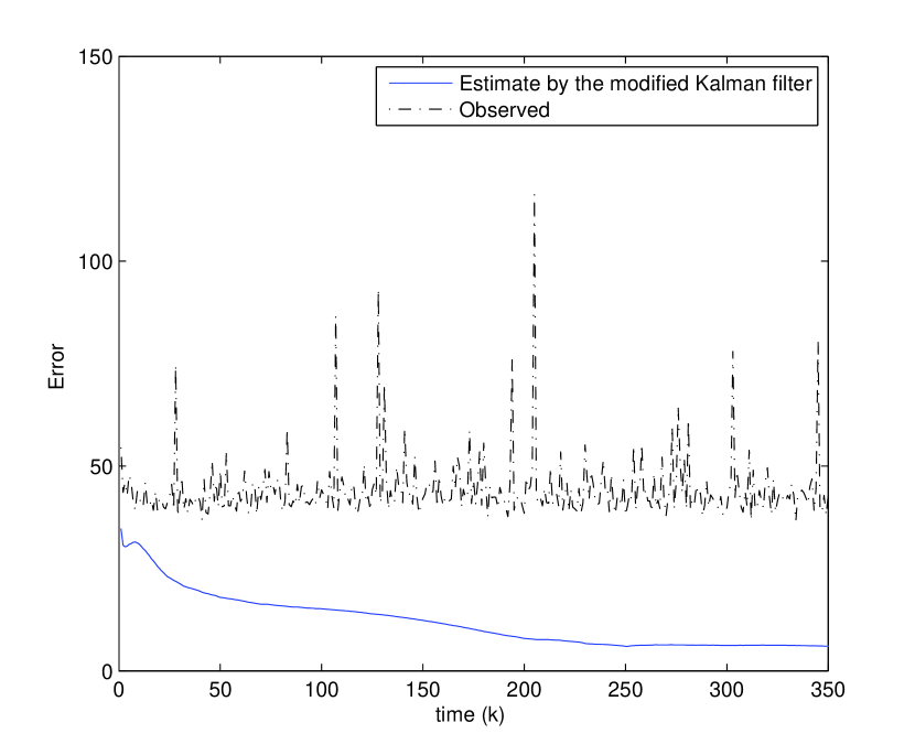
Take x01=10subscriptsuperscript𝑥1010x^{1}_{0}=10, x02=10subscriptsuperscript𝑥2010x^{2}_{0}=10, u01=1subscriptsuperscript𝑢101u^{1}_{0}=1, u02=0subscriptsuperscript𝑢200u^{2}_{0}=0, and we apply the modified Kalman filtering method to estimate xk1superscriptsubscript𝑥𝑘1x_{k}^{1} and xk2superscriptsubscript𝑥𝑘2x_{k}^{2}. In the simulation, the initial a priori estimate of the state, (x¯01subscriptsuperscript¯𝑥10\bar{x}^{1}_{0}, x¯02subscriptsuperscript¯𝑥20\bar{x}^{2}_{0}), is set to be equal to the observation at time 00, its error covariance, P¯0subscript¯𝑃0\bar{P}_{0}, is set to be unit matrix, and the threshold value C𝐶C is set to be 404040. The simulation results are shown in Figure 3, where the estimate position error, ER𝐸𝑅ER, defined by

ERk=(zk1xk1)2+(zk2xk2)2,𝐸subscript𝑅𝑘superscriptsubscriptsuperscript𝑧1𝑘subscriptsuperscript𝑥1𝑘2superscriptsubscriptsuperscript𝑧2𝑘subscriptsuperscript𝑥2𝑘2\displaystyle ER_{k}=\sqrt{(z^{1}_{k}-x^{1}_{k})^{2}+(z^{2}_{k}-x^{2}_{k})^{2}}, (27)

is compared with the observed position error, OR𝑂𝑅OR, defined by

ORk=(x¯k1xk1)2+(x¯k2xk2)2.𝑂subscript𝑅𝑘superscriptsubscriptsuperscript¯𝑥1𝑘subscriptsuperscript𝑥1𝑘2superscriptsubscriptsuperscript¯𝑥2𝑘subscriptsuperscript𝑥2𝑘2\displaystyle OR_{k}=\sqrt{(\bar{x}^{1}_{k}-x^{1}_{k})^{2}+(\bar{x}^{2}_{k}-x^{2}_{k})^{2}}. (28)

The results in Figure 3 are calculated by averaging 10,0001000010,000 times of simulations. It is seen from this figure that the position estimation error is significantly improved by using our modified Kalman filter.

In the simulation, we select C𝐶C by the method of trial and error, and it is found that the threshold value C𝐶C is not very picky and C𝐶C can vary from 303030 to 100100100 without significant effects on the performance of the modified Kalman filter. Determining the optimal C𝐶C, which is crucial for the modified Kalman filter, deserves further research and will be left for our future work.

References

  • [1] A. Ahn and R. Feldman. Optimal filtering of a gaussian signal in the presence of Lévy noise. SIAM Journal of Applied Mathematics, 60:359–369, 1999.
  • [2] D. Applebaum. Lévy Processes and Stochastic Calculus. Cambridge University Press, 2nd Edition, 2009.
  • [3] S. Asmussen and J. Rosinski. Approximation of small jumps of Lévy processes with a view towards simulation. Journal of Applied Probability, 38:482–493, 2001.
  • [4] A. Breton and M. Musiela. A generation of the kalman filter to models with infinite variance. Stochastic Processes and Applications, 47:75–94, 1993.
  • [5] R. Brown and P. Hwang. Introduction to Random Signals and Applied Kalman Filtering. John Wiley & Sons, 3rd Edition, 1997.
  • [6] M. Grewal and A. Andrews. Kalman Filtering: Theory and Practice Using Matlab. John Wiley & Sons, 3rd Edition, 2008.
  • [7] A. H. Jazwinski. Stochastic Processes and Filtering Theory. Academic Press, New York, 1970.
  • [8] A. Janicki and A. Weron. Simulation and Chaotic Behavior of αlimit-from𝛼\alpha-Stable Stochastic Processes, Marcel Dekker, Inc., 1994.
  • [9] D. Sornette and K. Ide. The Kalman-Lévy filter. Physica D, 151:142–174, 2001.
  • [10] W. A. Woyczynski. Lévy processes in the physical sciences. In Lévy Processes: Theory and Applications, O. E. Barndorff-Nielsen, T. Mikosch and S. I. Resnick (Eds.), 241-266, Birkhäuser, Boston, 2001.
Refer to caption
Figure 1: The usual Kalman filtering algorithm
Refer to caption
Figure 2: The modified Kalman filtering algorithm
Refer to caption
Figure 3: The error of the modified Kalman filtering algorithm