Towards Anisotropy-Free and Non-Singular Bounce Cosmology with Scale-invariant Perturbations

Abstract

We investigate non-singular bounce realizations in the framework of ghost-free generalized Galileon cosmology, which furthermore can be free of the anisotropy problem. Considering an Ekpyrotic-like potential we can obtain a total Equation-of-State (EoS) larger than one in the contracting phase, which is necessary for the evolution to be stable against small anisotropic fluctuations. Since such a large EoS forbids the Galileon field to generate the desired form of perturbations, we additionally introduce the curvaton field which can in general produce the observed nearly scale-invariant spectrum. In particular, we provide approximate analytical and exact semi-analytical expressions under which the bouncing scenario is consistent with observations. Finally, the combined Galileon-curvaton system is free of the Big-Rip after the bounce.

I Introduction

Non-singular bouncing cosmology Novello:2008ra has gained significant interest in recent studies of the early universe. The main reason for such a research direction is that the most popular paradigm of the early universe, namely inflation, still suffers from the “Big-Bang singularity” problem, which however can be naturally avoided in non-singular bouncing or cyclic cosmologies. Additionally, these paradigms can also solve the horizon, flatness and monopole problems, and make compatible observational predictions such as nearly scale-invariant power spectrum and moderate non-Gaussianities Cai:2007zv ; Cai:2008ed ; Qiu:2010ch . Therefore, they are recently considered as good alternatives to inflation.

In order to realize a successful bounce several requirements must be fulfilled. First of all, the basic condition is to have the Hubble parameter change its sign from negative to positive at the bounce, which implies that during the bouncing phase the Null Energy Condition (NEC) must be violated, with the total EoS of the universe going below $-1$ Cai:2007qw ; Cai:2009zp . The NEC violation in the context of General Relativity is nontrivial Nojiri:2013ru , usually leading to ghost degree(s) of freedom Carroll:2003st ; Cline:2003gs , which would demand either ghost-elimination mechanisms or an extended analysis to a modified gravity context Capozziello:2011et ; Biswas:2005qr .

Apart from the above basic condition, in order for a bounce to be a successful alternative to inflation it should also solve the other Big-Bang problems, and moreover it should produce a nearly scale-invariant power spectrum as required by observations Bennett:2012fp . These impose more stringent constraints on the bounce evolution, especially in the contracting phase. For instance, the horizon problem can be solved if the quantum fluctuations in the far past lie deep inside the horizon, while they should exit the horizon in the contracting phase in order to generate perturbations compatible with observations, provided that inflation is absent in bouncing scenario. This requires a total EoS satisfying $w>-1/3$ in the contracting phase Piao:2004jg ; Qiu:2012ia . However, the scale-invariance of the perturbations is even harder to be achieved. In particular, as it was initially shown in Finelli:2001sr , if the perturbations generated in the contracting phase are purely adiabatic, the EoS of the contracting universe should satisfy $w\approx 0$ in order to produce the desired spectrum.

However, although bounce models with total EoS $w\approx 0$ before the bounce, namely the “matter bounce”, could lead to nearly scale-invariant power spectrum, they generally suffer from the “anisotropy problem” Kunze:1999xp in the contracting phase. In particular, in 4D General Relativity a tiny amount of anisotropic fluctuation from the simple isotropic Friedmann-Robertson-Walker (FRW) geometry in the contracting phase, would increase as $a^{-6}$, where $a$ is the scale factor. Thus it would finally dominate over matter-like background, leading to a Big-Crunch singularity with complete anisotropy instead of a bounce, unless one impose a strong fine-tuning of the model parameters and the initial amount of anisotropy in order to obtain a bounce before the domination of the anisotropic term. In that sense the “matter bounce” scenario is not stable against cosmological anisotropy (for its similar problem in the presence of radiation see Karouby:2010wt ). For this reason, we must construct scenarios with total EoS larger than $1$ in order to prevent the dominance of anisotropy. However, as we mentioned above, a different EoS may not be able to provide the scale-invariant power spectrum, if we insist on applying the simple adiabatic mechanism of generating primordial perturbations. Therefore, we should resort to alternative mechanisms, such as adiabatic, entropy and conformal ones Khoury:2009my ; Finelli:2002we ; Lehners:2007ac ; Buchbinder:2007ad ; Lehners:2007wc ; Hinterbichler:2011qk .

In the present work we investigate the bounce realization in the framework of recently proposed generalized Galileon cosmology Nicolis:2008in ; Deffayet:2009mn (see also Silva:2009km ; DeFelice:2011bh for various developments). Due to the delicate design of the Lagrangian form such a theory, which contains higher-order derivatives, can keep its equation of motion up to second-order and thus is free of ghosts (this was pioneered by the work by Horndeski Horndeski:1974wa ), but it can indeed provide extra degree(s) of freedom in order to violate NEC. Recently, in Qiu:2011cy , the first ghost-free bounce model based on Galileon cosmology was constructed by one of the present authors and collaborators (see also Easson:2011zy ), and hence in this article we will consummate this class of models by addressing the problems mentioned above. Note that alternative scenarios addressing the anisotropy problem in Galileon bouncing cosmologies have been presented in Cai:2012va ; Cai:2013vm , of which before contracting with $w>1$, the universe can be dominated by cold matter Lin:2010pf , where scale-invariant perturbations could be generated.

First of all, by introducing an Ekpyrotic-like negative potential we can easily obtain a very large EoS in the contracting phase, thus the anisotropy problem will be eliminated. However, as mentioned above, a large EoS forbids the Galileon field to generate the desired form of perturbations, thus as a next step we additionally introduce the curvaton field which is suitably coupled to the Galileon field, such that the nearly scale-invariant spectrum can be produced. Finally, we perform a complete analysis of the behavior around the bounce point of the full Galileon-curvaton system, making use of the “inverse” reconstruction procedure Cai:2009in , showing that with a proper choice of the Lagrangian functional forms a non-singular bounce can be reconstructed, which can connect smoothly to the matter-domination era and moreover alleviate the Big-Rip singularity which appears in Qiu:2011cy .

The plan of the work is the following: In section II we briefly review the anisotropy problem. In section III we present the bouncing background evolution before, during and after the bounce, and we show that the perturbations are stable and free of ghosts. In section IV we analyze the curvaton mechanism that produces nearly scale-invariant perturbations. In section V we perform a semi-analytical procedure in order to reconstruct an exact bouncing solution that is not followed by a Big-Rip. Finally, in section VI we summarize and we discuss the obtained results. Throughout the manuscript we use the $(-,+,+,+)$ metric signature, and units in which $M_{Pl}=1/\sqrt{8\pi G}=1$.

II The anisotropy problem

The anisotropy problem is a notorious problem that generally exists in bouncing models with $w<1$ in contracting phase Kunze:1999xp . In General Relativity, if we allow the existence of a non-zero anisotropy at the beginning of the contraction it will evolve scaling as $a^{-6}(t)$. In order to demonstrate this more transparently, without loss of generality we consider as an example the simple anisotropic Bianchi-IX metric Misner:1974qy :

$$ds^{2}=-dt^{2}+a^{2}(t)\sum_{i=1}^{3}e^{2\beta_{i}(t)}d{x^{i}}^{2}~{},$$ (1)

with $\beta_{1}(t)+\beta_{2}(t)+\beta_{3}(t)=0$. The Friedmann Equation writes as:

$$3H^{2}=\rho_{u}+\frac{1}{2}\left(\sum_{i=1}^{3}\dot{\beta}_{i}^{2}\right)~{},$$ (2)

where $H=\dot{a}/a$ the Hubble parameter and with $\rho_{u}$ incorporating all the fluids in the universe. The $\beta_{i}$’s satisfy the equations

$$\ddot{\beta}_{i}+3H\dot{\beta}_{i}=0~{},$$ (3)

which provide the solutions $\beta_{i}\propto a^{-3}(t)$. Since the second part in the right hand side of equation (2) can be considered as an effective anisotropy term $\chi^{2}$, we conclude that

$$\chi^{2}\equiv\frac{1}{2}\left(\sum_{i=1}^{3}\dot{\beta}_{i}^{2}\right)\propto a^{-6}(t)~{},$$ (4)

and thus the anisotropy term corresponds to an effective energy density with EoS $w=1$. Although in an expanding universe this term is always sub-dominant and thus isotropization can be achieved, in a contracting case, as long as it is initially non-zero (even arbitrarily small), the anisotropy will grow fast and become dominant over all species with EoS less than 1, leading finally to a collapsing anisotropic universe. For this reason, in order to avoid the domination of a possible anisotropic fluctuation, one has to realize a contracting background that evolves even faster, which requires an EoS larger than unity in the contracting phase .

III The Galileon bounce

In the previous section we briefly showed that in order to realize a bounce we need an effective EoS $w>1$ in the contracting phase, in order to avoid the domination of an anisotropic fluctuation. In this section we formulate the bounce realization in generalized Galileon cosmology.

In the generalized Galileon scenario, where the coefficients of the various action-terms are considered as functions of the scalar field, the corresponding action can be written as Deffayet:2009mn :

$${\cal L}=\sum_{i=2}^{5}{\cal L}_{i}\,,$$ (5)

where

$${\cal L}_{2}=K(\phi,X)$$

$${\cal L}_{3}=-G_{3}(\phi,X)\Box\phi$$

$${\cal L}_{4}=G_{4}(\phi,X)\,R+G_{4,X}\,[(\Box\phi)^{2}-(\nabla_{\mu}\nabla_{\nu}\phi)\,(\nabla^{\mu}\nabla^{\nu}\phi)]$$

$${\cal L}_{5}=G_{5}(\phi,X)\,G_{\mu\nu}\,(\nabla^{\mu}\nabla^{\nu}\phi)$$

$$\ \ \ \ \ \ \ -\frac{1}{6}\,G_{5,X}\left[(\Box\phi)^{3}-3(\Box\phi)\,(\nabla_{\mu}\nabla_{\nu}\phi)\,(\nabla^{\mu}\nabla^{\nu}\phi)\right.$$

$$\left.\ \ \ \ \ \ \ \ \ \ \ \ \ \ \ \ \ \ \ \ +2(\nabla^{\mu}\nabla_{\alpha}\phi)\,(\nabla^{\alpha}\nabla_{\beta}\phi)\,(\nabla^{\beta}\nabla_{\mu}\phi)\right]\,.$$ (6)

In this action the functions $K$ and $G_{i}$ ($i=3,4,5$) depend on the scalar field $\phi$ and its kinetic energy $X\equiv-\frac{1}{2}\nabla_{\mu}\phi\nabla^{\mu}\phi$, while $R$ is the Ricci scalar and $G_{\mu\nu}$ is the Einstein tensor. Moreover, $G_{i,X}$ and $G_{i,\phi}$ ($i=3,4,5$) denote the partial derivatives of $G_{i}$ with respect to $X$ and $\phi$, ($G_{i,X}\equiv\partial G_{i}/\partial X$ and $G_{i,\phi}\equiv\partial G_{i}/\partial\phi$), and the box operator is constructed from covariant derivatives: $\Box\phi\equiv g^{\mu\nu}\nabla_{\mu}\nabla_{\nu}\phi$. In the following we focus on the case

$$K(\phi,X)=X-V(\phi),~{}G_{3}(\phi,X)=g(\phi)X,$$

$$G_{4}(\phi,X)=\frac{1}{2},~{}G_{5}(\phi,X)=0.$$ (7)

Therefore, the action that we are going to use reads:

$${\cal S}=\int d^{4}x\sqrt{-g}\left[\frac{1}{2}R-\frac{1}{2}\nabla_{\mu}\phi\nabla^{\mu}\phi-V(\phi)\right.\ \ \ \ \ \ \ \ \ \ \ \$$

$$\left.\ \ \ \ \ \ \ \ \ \ \ \ \ \ \ \ \ \ \ \ \ \ +\frac{g}{2}\nabla_{\mu}\phi\nabla^{\mu}\phi\Box\phi\right].$$ (8)

We now proceed to a detailed investigation of the above scenario. Firstly, in the following subsection we provide approximate analytical solutions at the far past before the bounce, around the bouncing regime, and after the bounce, at the background level. Then in the next subsection, we analyze the perturbation behavior.

III.1 Background evolution: analytical results

In the following we impose a flat Friedmann-Robertson-Walker (FRW) background metric of the form $ds^{2}=-N^{2}(t)dt^{2}+a^{2}(t)d{\bf{x}}^{2}$, where $t$ is the cosmic time, $x^{i}$ are the comoving spatial coordinates, $N(t)$ is the lapse function, and $a(t)$ is the scale factor. Varying the action (III) with respect to $N(t)$ and $a(t)$ respectively, and setting $N=1$, we obtain the Friedmann equations

$$H^{2}=\frac{1}{3}\rho~{},~{}~{}~{}\dot{H}=-\frac{1}{2}(\rho+P)~{}.$$ (9)

Additionally, we have defined the effective energy density and pressure as:

$$\rho = \frac{1}{2}\dot{\phi}^{2}+V(\phi)+3gH\dot{\phi}^{3}~{},$$ (10)

$$P = \frac{1}{2}\dot{\phi}^{2}-V(\phi)-g\dot{\phi}^{2}\ddot{\phi}~{},$$ (11)

and thus the total EoS of the universe is just

$$w\equiv\frac{P}{\rho}=\frac{\dot{\phi}^{2}-2V(\phi)-2g\dot{\phi}^{2}\ddot{\phi}}{\dot{\phi}^{2}+2V(\phi)+6gH\dot{\phi}^{3}}~{}.$$ (12)

Finally, variation of (III) with respect to the Galileon field provides its evolution equation:

$$\mathcal{D}\ddot{\phi}+\Gamma\dot{\phi}+V_{\phi}=0~{},$$ (13)

where

$$\mathcal{D} = 1+6gH\dot{\phi}+\frac{3}{2}g^{2}\dot{\phi}^{4}~{},$$ (14)

$$\Gamma = \frac{3}{2}\left(1+3gH\dot{\phi}\right)\left(2H-g\dot{\phi}^{3}\right)~{}.$$ (15)

In the following we will suitably choose the potential $V(\phi)$ in order to obtain a very large positive equation of state in relation (12), namely $w>1$, so that our model will not suffer from the anisotropy problem in the contracting phase. Meanwhile, when the Galileon term $G\Box\phi$ becomes more and more important, the EoS becomes negative and eventually triggers the bounce.

As a specific example, we choose the potential to be

$$V(\phi)=-V_{0}e^{c\phi},$$ (16)

with $V_{0},c>0$, namely a negative exponential potential, which is the usual one in Ekpyrotic scenarios Khoury:2001wf . Within this choice, when the nonlinear kinetic term is relatively small we obtain $\rho<P$ and thus $w>1$. One could ask whether the negative potential would lead to a negative energy density, however the more negative the potential is, the steeper it is, and thus it gives rise to larger kinetic term, which can compensate the potential negativity (this will be verified later on).

Let us proceed to a qualitative investigation of the dynamics of such scenario. For simplicity we consider that $\phi$ increases from negative to positive during the evolution, therefore at the beginning when $\phi$ starts at a large negative value the potential (16) is in its “slow-varying” region, and the field moves slowly. In this region the nonlinear term $G\Box\phi$ will have a small contribution to the action. Similarly to the Ekpyrotic models, the universe will contract with a very large positive EoS, but as time passes $\phi$ moves towards positive values and its velocity increases, the effect of the $G\Box\phi$ term is enhanced, and it can trigger the bounce. However, after the bounce and due to the large slope of the potential, the field kinetic energy could increase to unacceptably large values which could spoil the validity of the effective theory. Therefore, we should need some mechanisms to slow the field motion down, and this will be demonstrated in detail in the next sections.

In the following we proceed to the quantitative investigation of the scenario, extracting approximate analytical solutions for the background evolution in the far past before the bounce, around the bouncing point, and in the far future after the bounce.

III.1.1 Solution far before the bounce

Far before the bounce, as we assumed, $\phi$ begins with a large negative value and moves slowly, while the nonlinear term of $\dot{\phi}$ is negligible. The energy density and pressure reduces to

$$\rho\simeq\frac{1}{2}\dot{\phi}^{2}+V(\phi)~{},~{}P\simeq\frac{1}{2}\dot{\phi}^{2}-V(\phi)~{},$$ (17)

similarly to a single scalar field with an Ekpyrotic potential. Thus, we can choose the model parameters and the initial conditions of $\phi$ in order to acquire scaling solutions, namely to obtain a scale factor evolving as

$$a(t)\sim(t_{\ast}-t)^{p}\sim|\eta_{\ast}-\eta|^{\frac{p}{1-p}}~{},~{}\ \ p\equiv\frac{2}{3(1+w)},~{}$$ (18)

where the subscript ‘$\ast$’ denotes the time where the non-linear term in equations (10)-(13) becomes important. Note that since we are considering the region where $t<t_{\ast}$, we have $t_{\ast}-t>0$. For completeness we have also expressed the above solution using the conformal time $\eta$, related to the cosmic time $t$ through $dt=ad\eta$. Similarly, the field $\phi(t)$ scales as

$$\phi(t)\simeq-\frac{2}{c}\ln(t_{\ast}-t)~{},~{}p=\frac{2}{c^{2}}~{}.$$ (19)

Moreover, taking the derivatives of the above expressions we find

$$\dot{\phi}(t)\simeq\frac{2}{c(t_{\ast}-t)},$$ (20)

$$H(t)\simeq\frac{p}{t-t_{\ast}}~{},$$ (21)

and therefore the energy density from expression (10) becomes

$$\rho(t)_{t<t_{\ast}}=3H^{2}\propto(t-t_{\ast})^{-2}$$ (22)

Finally, using relations (18) and (19), for the total EoS using (12) we obtain

$$w\simeq\frac{1}{3}c^{2}-1=const.$$ (23)

III.1.2 Solution around the bounce

Around the bouncing point $t_{B}$ the nonlinear term becomes important. From the Friedmann equation (9) we can express $H$ as:

$$H=\frac{1}{2}g\dot{\phi}^{3}\pm\frac{1}{6}\sqrt{9g^{2}\dot{\phi}^{6}+6(\dot{\phi}^{2}-2V_{0}e^{c\phi})}~{},$$ (24)

in which the nonlinear term becomes important and the last terms in (10) and (11) can no longer be neglected. Without loss of generality we can keep the minus-sign branch in order to obtain a positive $\dot{\phi}(t)$. Therefore, when the universe goes from the contracting ($H<0$) to the expanding phase ($H>0$), one has $\dot{\phi}>\sqrt{2V_{0}}e^{c\phi/2}$ before and $\dot{\phi}<\sqrt{2V_{0}}e^{c\phi/2}$ after the bounce. It is therefore natural to consider the solution at the bounce region to be

$$\dot{\phi}=\sqrt{2V_{0}}(\alpha t+\beta)e^{\frac{c\phi}{2}}~{},$$ (25)

with $\alpha$ and $\beta$ being two parameters satisfying the conditions

$$\alpha<0~{},~{}\alpha t_{B}+\beta=1~{}.$$ (26)

Note that substitution of (25) into the $\phi$-equation of motion (13), provides the necessary value for the coefficient $\alpha$ in order to have self-consistency.

Integrating equation (25) leads to

$$e^{-\frac{c\phi_{0}}{2}}-e^{-\frac{c\phi}{2}}=\sqrt{2V_{0}}\Big{[}\frac{\alpha}{2}(t_{0}^{2}-t^{2})+\beta(t_{0}-t)\Big{]}~{},$$ (27)

with $t_{0}$ a boundary value for $t$, and $\phi_{0}$ the corresponding value of $\phi$. The above formula will be simplified if we set $t_{0}$ in the far future when $\phi_{0}$ becomes very large, and thus $e^{-\frac{c\phi_{0}}{2}}\approx 0$. In this case the expression for $\phi(t)$ becomes

$$\phi=-\frac{2}{c}\ln\Big{\{}-\sqrt{2V_{0}}(t_{0}-t)\Big{[}\frac{\alpha}{2}(t-t_{0})+\alpha t_{0}+\beta\Big{]}\Big{\}}~{},$$ (28)

which leads to

$$\dot{\phi} = \frac{4(\alpha t+\beta)}{c(t_{0}-t)[\alpha(t-t_{0})+2(\alpha t_{0}+\beta)]}~{},$$ (29)

$$\ddot{\phi} = \frac{2}{c}\left\{\frac{1}{(t_{0}-t)^{2}}+\frac{\alpha^{2}}{[\alpha(t+t_{0})+2\beta]^{2}}\right\}~{}.$$ (30)

It would be useful if we could approximate the above expressions around the bouncing point $t_{B}$, namely $t\rightarrow t_{B}=(1-\beta)/\alpha$. In this case, and neglecting the constant terms in order to extract the pure scaling behavior, we obtain

$$\phi\simeq\frac{4\alpha(t-t_{B})}{c\left[(\beta+\alpha t_{0})^{2}-1\right]},$$

$$\dot{\phi}\simeq\frac{4\alpha^{2}\left[(\beta+\alpha t_{0})^{2}+1\right](t-t_{B})}{c\left[(\beta+\alpha t_{0})^{2}-1\right]^{2}},$$

$$\ddot{\phi}\simeq\frac{8\alpha^{3}\left[3(\beta+\alpha t_{0})^{2}+1\right](t-t_{B})}{c(\beta+\alpha t_{0}-1)^{3}(\beta+\alpha t_{0}+1)^{3}},$$ (31)

that is $\phi$ exhibits a linear behavior around $t_{B}$. Following the same way, one could also insert these expressions into equation (24) and (12) to straightforwardly obtain the approximate solutions for $H(t)$ and $w(t)$, respectively.

III.1.3 Solution after the bounce

Far after the bounce, when $t$ approaches $t_{0}$, the solutions are still given by (28)-(30). Thus, approximating them at $t\rightarrow t_{0}$, and neglecting the constant terms in order to extract the pure scaling behavior, we acquire

$$\phi \simeq -\frac{2}{c}\ln(t_{0}-t)~{},$$ (32)

$$\dot{\phi} \simeq \frac{2}{c}\frac{1}{t_{0}-t}~{},$$ (33)

$$\ddot{\phi} \simeq \frac{2}{c}\frac{1}{(t_{0}-t)^{2}}~{}.$$ (34)

In this case, inserting these expressions into (24), we can extract a simple approximate expression for $H(t)$ too, namely

$$H\simeq\frac{1}{(t_{0}-t)^{3}}~{},$$ (35)

which leads to a Big-Rip singularity when $t$ approaches $t_{0}$. This can be easily explained since when the nonlinear terms become very important the last terms in (10) and (11) become dominant. Thus, when the energy density is dominated by the $3gH\dot{\phi}^{3}$ term, namely $3H^{2}=\rho\sim 3gH\dot{\phi}^{3}$, we straightforwardly find that the Hubble parameter $H$ will be proportional to $\dot{\phi}^{3}$, and (35) is verified. Finally, the total EoS can also be obtained by inserting these expressions into (12).

III.1.4 Numerical verification

Figure 1: The evolution of the Galileon field $\phi$ with respect to $t$. We choose the initial conditions to be $\phi_{i}=-\sqrt{3}(\ln 20)/3$ and $\dot{\phi}_{i}=\sqrt{3}/60$, and the parameters to be $c=2\sqrt{3}$, $g=1$, and $V_{0}=1/12$, respectively.

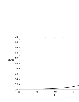
Figure 2: The evolution of the speed of the Galileon field $\dot{\phi}$ with respect to $t$. We choose the initial conditions to be $\phi_{i}=-\sqrt{3}(\ln 20)/3$ and $\dot{\phi}_{i}=\sqrt{3}/60$, and the parameters to be $c=2\sqrt{3}$, $g=1$, and $V_{0}=1/12$, respectively.

Figure 3: The evolution of the Hubble parameter $H$ with respect to $t$. We choose the initial conditions to be $\phi_{i}=-\sqrt{3}(\ln 20)/3$ and $\dot{\phi}_{i}=\sqrt{3}/60$, and the parameters to be $c=2\sqrt{3}$, $g=1$, and $V_{0}=1/12$, respectively.

Figure 4: The evolution of the EoS $w$ with respect to $t$. We choose the initial conditions to be $\phi_{i}=-\sqrt{3}(\ln 20)/3$ and $\dot{\phi}_{i}=\sqrt{3}/60$, and the parameters to be $c=2\sqrt{3}$, $g=1$, and $V_{0}=1/12$, respectively.

Figure 5: The evolution of the total energy density $\rho$ of the Galileon field, with respect to $t$. We choose the initial conditions to be $\phi_{i}=-\sqrt{3}(\ln 20)/3$ and $\dot{\phi}_{i}=\sqrt{3}/60$, and the parameters to be $c=2\sqrt{3}$, $g=1$, and $V_{0}=1/12$, respectively.

We close the background investigation by performing an exact numerical elaboration in order to verify the above approximate expressions in the various regimes. In particular, we numerically solve equations (9) and (13), imposing (19) as our initial conditions. In Figures 1, 2, 3 and 4, we respectively present $\phi(t)$, $\dot{\phi}(t)$, the Hubble parameter $H(t)$ as well as the EoS $w(t)$. As we observe, both $\phi(t)$ and $\dot{\phi}(t)$ are monotonically increasing. Moreover, before the bounce the universe contracts with a scaling solution with EoS $w$ being constant and larger than unity (in this specific example $w=3$), and thus the scenario is free from the anisotropy problem discussed in section II.

As time passes the nonlinear term becomes important and triggers the bounce, which forces $H(t)$ to change from negative to positive. Note that the numerical results confirm that $\dot{\phi}(t)$ has a positive value during the bouncing period, and thus it justifies our choice of the minus sign in (24). After the bounce, the nonlinear kinetic term makes the scalar-field energy density increasing, leading the universe to a Big-Rip. One can also see that the total EoS $w(t)$ indeed indicates the bounce followed by the Big-Rip, verifying the analytical results that has been obtained in preceding paragraphs.

Finally, in Fig. 5, we present the evolution of the total energy density $\rho$ of the Galileon field, calculated through (10). As we observe $\rho$ is always positive, despite the use of a negative potential, due to the increase of the kinetic energy, and it becomes zero only at the bounce point as expected. Therefore, in the present work we do not need mechanisms that could transit the universe to positive potential energy Felder:2002jk , however it would be desirable to consider a mechanism that could smooth the increase of the Galileon kinetic energy, by either considering a bound in the potential, or couple $\phi$ to other matter fields such is radiation, which could lead to energy transfer away from it (a procedure that could lead to the universe preheating too). These mechanisms lie beyond the scope of the present work and are left for a future investigation.

III.2 Perturbations

In the previous subsection we analyzed the background evolution of the Galileon bounce. Thus, we can now proceed to the investigation of the perturbations, focusing on their stabilities. It proves convenient to foliate the FRW metric in an Arnowitt-Deser-Misner (ADM) form Arnowitt:1962hi :

$$ds^{2}=-N^{2}dt^{2}+h_{ij}(dx^{i}+N^{i}dt)(dx^{j}+N^{j}dt)~{},$$ (36)

where $N$ is the lapse function, $N^{i}$ is the shift vector, and $h_{ij}$ is the induced 3-metric. One can then perturb these functions as:

$$N=1+A~{},~{}N_{i}=\partial_{i}\psi~{},~{}h_{ij}=a^{2}(t)e^{2\zeta}\delta_{ij}~{},$$ (37)

where $A$, $\psi$ and $\zeta$ are the scalar metric perturbations. As usual it is useful to define the (gauge-invariant) comoving curvature perturbation through

$$\mathcal{R}\equiv\zeta+\frac{H}{\dot{\phi}}\delta\phi~{},$$ (38)

and hence in the uniform $\phi$ gauge we acquire $\delta\phi=0$ and $\zeta=\mathcal{R}$.

Under the above perturbation scheme, the action (III) perturbed up to second order becomes:

$$\mathcal{S}^{(2)}=\int d\eta d^{3}xa^{2}\frac{Q_{\cal R}}{c_{s}^{2}}\Bigl{[}{\cal R}^{\prime 2}-c_{s}^{2}(\partial{\cal R})^{2}\Bigr{]}~{},$$ (39)

where $\eta$ is the conformal time. In the above expression we have introduced the sound-speed squared $c_{s}^{2}$, and the quantity $Q_{\cal R}$ related to instabilities, which in our specific scenario read as

$$c_{s}^{2} = Q_{\cal R}^{-1}[1+2g(\ddot{\phi}+2H\dot{\phi})-\frac{1}{2}g^{2}\dot{\phi}^{4}]~{},$$ (40)

$$Q_{\cal R} = 1+6gH\dot{\phi}+\frac{3}{2}g^{2}\dot{\phi}^{4}~{}.$$ (41)

Figure 6: The evolution of the squared speed of sound $c_{s}^{2}$ with respect to $t$. We choose the initial conditions to be $\phi_{i}=-\sqrt{3}(\ln 20)/3$ and $\dot{\phi}_{i}=\sqrt{3}/60$, and the parameters to be $c=2\sqrt{3}$, $g=1$, and $V_{0}=1/12$, respectively.

Note that according to the definition of $\mathcal{D}$ in (14) we obtain $2Q_{\cal R}=\mathcal{D}$.

The perturbative action (39) could in principle lead to ghosts and gradient instabilities, which would be catastrophic since it is this action that can be written as a canonical form and then be quantized. From its form one can see that the avoidance of ghosts requires the factor in front of the kinetic term of the perturbation variable ${\cal R}$ to be positive, namely $Q_{R}/c_{s}^{2}>0$, while the absence of gradient instabilities requires $c_{s}^{2}\geq 0$ DeFelice:2011bh , which means the ratio of the factors of spatial and time derivatives must be positive. In order to show that this is the case for the exact behavior too, in Figures 6 and 7 we respectively depict $c_{s}^{2}$ and $Q_{\cal R}$, arising from the numerical elaboration of the full system.

Figure 7: The evolution of the instability-related quantity $Q_{\cal R}$ with respect to $t$. We choose the initial conditions to be $\phi_{i}=-\sqrt{3}(\ln 20)/3$ and $\dot{\phi}_{i}=\sqrt{3}/60$, and the parameters to be $c=2\sqrt{3}$, $g=1$, and $V_{0}=1/12$, respectively.

From the above analysis we can see that our model is stable under both ghost and gradient instabilities. However, it generally generates a (deep) blue tilted power spectrum, which cannot be consistent with observations. Note that in Qiu:2011cy this was shown for $w=1/3$, therefore in our present case where $w>1$ the blue tilt of the power spectrum is even stronger. This implies that the anisotropy-free requirement $w>1$ and the scale-invariant perturbation generation cannot be obtained simultaneously in the current case, as was already mentioned in the Introduction. For this reason, we should introduce an additional mechanism in order to be able to generate the nearly invariant perturbation spectrum, without spoiling the solution to the anisotropy problem. This can be performed by the curvaton mechanism, as we will present in the next section.

IV The curvaton mechanism and the Scale-invariant spectrum

In the previous section we showed that the Galileon scenario under an Ekpyrotic-like potential can exhibit a bouncing solution naturally. In the contracting phase the corresponding total EoS of the universe satisfies $w>1$ in order for the evolution to be free of the anisotropy problem discussed in section II. However, under this requirement the corresponding perturbations, although free of ghost and gradient instabilities, cannot give rise to a nearly scale-invariant power spectrum, as it is required by observational data Bennett:2012fp .

In Qiu:2011cy it was shown that this problem can be solved by introducing a curvaton field $\sigma$ coupled to the Galileon $\phi$. As it is usual for curvaton fields Lyth:2001nq , $\sigma$ does not affect the bouncing background behavior, but it can lead to a power spectrum in agreement with observations. In particular, through a specific Galileon-curvaton coupling, the curvaton field lies effectively in a “fake” de-Sitter expansion or matter-like contraction, and thus it can generate a nearly scale-invariant power spectrum. This is the idea behind the “conformal” mechanism Hinterbichler:2011qk and in this section we investigate the necessary form of the coupling functions.

Let us consider the curvaton action as

$${\cal S}_{\sigma}=\frac{1}{2}\int d^{4}x\sqrt{-g}[-{\cal F}(\phi)(\partial\sigma)^{2}-2{\cal G}(\phi)W(\sigma)]~{},$$ (42)

allowing for the most general form of coupling between $\sigma$ and $\phi$. The functions ${\cal F(\phi)}$ and ${\cal G(\phi)}$ depend on $\phi$, while $W(\sigma)$ is the potential for $\sigma$. Variation of action (42) with respect to $\sigma$ gives its background evolution equation as:

$$\ddot{\sigma}_{0}+\frac{(a^{3}{\cal F})^{\cdot}}{a^{3}{\cal F}}\dot{\sigma}_{0}+\frac{{\cal G}}{{\cal F}}W_{\sigma_{0}}=0~{},$$ (43)

where $\sigma_{0}$ is the background value of $\sigma$ and $W_{\sigma_{0}}$ corresponds to $\partial W/\partial\sigma|_{\sigma_{0}}$. In the following, and up to the end of this section, we omit the subscript “0”, denoting the background by a simple $\sigma$, unless explicitly mentioned. Additionally, the energy density and pressure of $\sigma$ can be respectively written as:

$$\rho_{\sigma}=\frac{1}{2}{\cal F}\dot{\sigma}^{2}+{\cal G}W~{},~{}P_{\sigma}=\frac{1}{2}{\cal F}\dot{\sigma}^{2}-{\cal G}W~{}.$$ (44)

We now proceed to the examination of the perturbations generated from the curvaton field. Perturbing it by $\delta\sigma$ and defining $u\equiv a\sqrt{{\cal F}}\delta\sigma$, we can extract the corresponding perturbation equation as a second-order differential equation:

$$u^{\prime\prime}+\left(k^{2}+a^{2}\frac{{\cal G}}{{\cal F}}W_{\sigma\sigma}-\frac{z^{\prime\prime}}{z}\right)u=0~{},$$ (45)

where the prime denotes derivative with respect to the conformal time $\eta$, $W_{\sigma\sigma}\equiv\partial^{2}W(\sigma)/(\partial\sigma)^{2}$ is the second derivative of the potential with respect to $\sigma$, and we have defined $z\equiv a\sqrt{\cal F}$. As usual, the power spectrum generated by $\delta\sigma$ is defined as:

$${\cal P}_{\delta\sigma}=\frac{k^{3}}{2\pi^{2}}\Big{|}\frac{u}{z}\Big{|}^{2}~{}.$$ (46)

Therefore, we deduce that the condition for obtaining a scale-invariant power spectrum of $\delta\sigma$ is:

$$\frac{a^{2}{\cal G}W_{\sigma\sigma}}{\cal F}-\frac{z^{\prime\prime}}{z}\simeq-\frac{2}{|\eta_{\ast}-\eta|^{2}}~{}.$$ (47)

There are several ways to satisfy the condition (47). The simplest one is to set $W(\sigma)=0$, in which the first term in the above condition disappears, and thus we need just to suitably choose ${\cal F}$ in order to obtain $z^{\prime\prime}/z\simeq 2|\eta_{\ast}-\eta|^{-2}$. Alternatively we can incorporate the effects of both the kinetic and the potential terms of $\sigma$. In the following subsections we consider these cases separately.

IV.1 $W(\sigma)=0$

Under $W(\sigma)=0$, the condition (47) of obtaining scale-invariant power spectrum becomes

$$z\propto|\eta_{\ast}-\eta|^{2}\,\,\,{\text{or}}\,\,\,|\eta_{\ast}-\eta|^{-1}~{}.$$ (48)

For the case of $z\propto|\eta_{\ast}-\eta|^{2}$ we obtain

$$\delta\sigma=\frac{u}{z}\sim k^{\frac{3}{2}}~{},~{}~{}~{}k^{-\frac{3}{2}}|\eta_{\ast}-\eta|^{-3}~{},$$ (49)

the latter of which dominates over the former. Therefore, using expression (46) we can obtain the power spectrum as

$${\cal P}_{\delta\sigma}\sim k^{0}|\eta_{\ast}-\eta|^{-6}~{}.$$ (50)

As we observe, the spectrum is indeed scale-invariant but it has an increasing amplitude.

On the other hand, for the case of $z\propto|\eta_{\ast}-\eta|^{-1}$ we acquire

$$\delta\sigma=\frac{u}{z}\sim k^{-\frac{3}{2}}~{},~{}~{}~{}k^{\frac{3}{2}}|\eta_{\ast}-\eta|^{3}~{},$$ (51)

the former of which dominates over the latter. Therefore, using (46) we can obtain the power spectrum as

$${\cal P}_{\delta\sigma}\sim k^{0}.$$ (52)

In this case the spectrum is scale-invariant and moreover it is conserved on super-horizon scales.

The absence of $W(\sigma)$ leads to an absence of ${\cal G}(\phi)$ too. Thus, we only need to suitably determine the form of ${\cal F}(\phi)$ according to the condition (48). Note that far before the bounce we have already assumed the scale-factor ansatz (18), and therefore (48) requires just

$${\cal F}\propto|\eta_{\ast}-\eta|^{\frac{2(2-3p)}{1-p}}\,\,\,{\text{or}}\,\,\,|\eta_{\ast}-\eta|^{\frac{2}{p-1}}~{}.$$ (53)

Furthermore, from the ansatz solution (19) for $\phi$ and the above expressions we deduce that the suitable choice of the form of ${\cal F}$ in terms of $\phi$ might be

$${\cal F}\propto e^{2(3-c^{2})\phi/c}\,\,\,{\text{or}}\,\,\,e^{c\phi}~{},$$ (54)

where we have made use of the relation $p=2/c^{2}$ (note that since in contracting phase $w\gg 1$, we have $0<p\ll 1$).

We close this subsection by examining the backreaction of $\sigma$ field on the background evolution, since although the curvaton is necessary for the correct perturbation generation we would not desire it to spoil the background bouncing behavior itself. In the contraction region where $t<t_{\ast}$, the background energy density of the system scales as $\rho_{t<t_{\ast}}\sim(t_{\ast}-t)^{-2}$, as it was found in (22). On the other hand, the evolution equation of the curvaton field (43) gives $\dot{\sigma}\sim a^{-3}{\cal F}^{-1}$, and thus its energy density in (44) becomes $\rho_{\sigma}\simeq{\cal F}\dot{\sigma}^{2}/2\sim a^{-6}{\cal F}^{-1}$. Since we know the time-dependence of the scale factor from (18) and the time-dependence of ${\cal F}$ from (53), we straightforwardly deduce that for the solution branch where $z\propto|\eta_{\ast}-\eta|^{2}$ we obtain $\rho_{\sigma}\sim(t_{\ast}-t)^{-4}$, while for the solution branch where $z\propto|\eta_{\ast}-\eta|^{-1}$ we acquire $\rho_{\sigma}\sim(t_{\ast}-t)^{2(1-3p)}\sim(t_{\ast}-t)^{2}$ (in the last step we used that $p\ll 1$). Therefore, our analysis indicates that in the solution branch where $z\propto|\eta_{\ast}-\eta|^{2}$ (with ${\cal F}\propto e^{2(3-c^{2})\phi/c})$, one has to suitably tune the initial conditions in order for the curvaton not to destroy the background bouncing behavior. However, in the second solution branch where $z\propto|\eta_{\ast}-\eta|^{-1}$ (with ${\cal F}\propto e^{c\phi})$, the energy density of the curvaton field grows slower than that of the background, and thus the background bouncing evolution is not altered by the backreaction of the curvaton.

IV.2 $W(\sigma)\neq 0$

We now examine the case where the curvaton potential is non-zero, in order to investigate its effect on the perturbation generation. Without loss of generality and for simplicity we assume that ${\cal F}$ is approximately a constant (we set ${\cal F}=1$), although extension to general ${\cal F}$ is straightforward.

In order to see what condition (47) gives in this case, we recall that at the early stage of the bouncing phase, where the perturbation $\delta\sigma$ is generated, the scale factor evolves according to (18), and therefore since $z\equiv a\sqrt{{\cal F}}$ we obtain

$$\frac{z^{\prime\prime}}{z}=\frac{a^{\prime\prime}}{a}\simeq\frac{p}{1-p}\left(\frac{p}{1-p}-1\right)\frac{1}{\left|\eta-\eta_{\ast}\right|^{2}}~{}.$$ (55)

Furthermore, introducing $a_{\ast}=a(\eta_{\ast})$ we can write

$$a^{2}\frac{{\cal G}}{{\cal F}}W_{,\sigma\sigma}=a_{\ast}^{2}{\cal G}W_{,\sigma\sigma}\left|\eta_{\ast}-\eta\right|^{\frac{2p}{1-p}}~{}.$$ (56)

Inserting equations (55) and (56) into (47) we deduce that the condition for obtaining a scale-invariant power spectrum of $\delta\sigma$ becomes

$$a_{\ast}^{2}{\cal G}W_{\sigma\sigma}=\frac{3p-2}{(1-p)^{2}}\left|\eta_{\ast}-\eta\right|^{-\frac{2}{1-p}}~{}.$$ (57)

As a specific example we consider the well-studied case of a quadratic potential, namely $W(\sigma)=m_{\sigma}^{2}\sigma^{2}/2$, in which case $W_{\sigma\sigma}=const$. Hence, condition (57), using also the $\phi$-evolution from (19), gives

$${\cal G}\propto e^{c\phi}~{}.$$ (58)

Therefore, we extract that the field perturbation $\delta\sigma$ scales as:

$$\delta\sigma=\frac{u}{z}\sim k^{-\frac{3}{2}}|\eta_{\ast}-\eta|^{\frac{1}{p-1}}~{},~{}~{}~{}k^{\frac{3}{2}}|\eta_{\ast}-\eta|^{\frac{3p-2}{p-1}}~{}.$$ (59)

We mention that since we assume ${\cal F}=1$ (that is $z=a$) the “fake” effect is absent, and thus the dominating mode of the perturbations is always the growing mode.

We close this subsection by examining the backreaction of $\sigma$ field on the background evolution, since we would not want the curvaton to spoil the background bouncing behavior itself. The $\sigma$-evolution equation (43) becomes

$$\ddot{\sigma}+3H\dot{\sigma}+m_{\sigma}^{2}{\cal G}\sigma=0~{}.$$ (60)

Since according to relations (58) and (19) we have ${\cal G}\sim e^{c\phi}\sim(t_{\ast}-t)^{-2}$, we can write ${\cal G}={\cal G}_{0}(t_{\ast}-t)^{-2}$ with ${\cal G}_{0}$ being an arbitrary constant. Therefore, equation (60) accepts the solution

$$\sigma\sim(t_{\ast}-t)^{\frac{1}{2}[1-3p\pm\sqrt{(1-3p)^{2}-4m_{\sigma}^{2}{\cal G}_{0}}]}~{}.$$ (61)

Finally, substituting it into (44) for the curvaton energy density we obtain

$$\rho_{\sigma}\sim(t_{\ast}-t)^{[1-3p\pm\sqrt{(1-3p)^{2}-4m_{\sigma}^{2}{\cal G}_{0}}]-2}~{}.$$ (62)

Comparing the background energy-density evolution (22) with the curvaton energy-density evolution (62) we deduce that the requirement for the latter to grow slower than the former is to have $1-3p\pm\sqrt{(1-3p)^{2}-4m_{\sigma}^{2}{\cal G}_{0}}>0$. However, since in order to solve the anisotropy problem we focus on $w>1$ (or equivalently $p<1/3$), then provided ${\cal G}_{0}>0$ the above requirement is always satisfied. Therefore, in the scenario at hand the energy density of the curvaton field will never dominate over the background evolution, that is the background bouncing behavior will not be destroyed by its backreaction.

We close this section with a comment on the preservation of the scale invariance across and after the bounce, which is in general a crucial question in bouncing scenarios, and on the matching conditions we impose. In the above analysis we required $\delta\sigma$ and $\delta\sigma^{\prime}$ to be continuous across the bounce, which is consistent with Deruelle-Mukhanov matching conditions Deruelle:1995kd . Considering the expanding phase, since it usually contains two modes, namely the constant and the growing/decaying one, the perturbation spectrum may or may not get altered depending on whether mode-mixing is realized or not, or depending on whether the varying modes in contracting/expanding phase are growing/decaying, which is determined by the background. For instance, in the above case where ${\cal F}(\phi)\sim e^{c\phi}$ and $W(\sigma)=0$, the contracting modes are decaying, thus by using the aforementioned matching conditions scale-invariance will be maintained if the expanding mode is growing, which requires the background EoS (or the effective EoS, if there is a “faking”) to be no larger than 1, and therefore we may easily preserve the scale-invariance in the expanding phase by slightly constraining the background evolution. A more detailed discussion on these will be taken on in a following-up paper. Similar results can be found in Cai:2012va .

V Reconstructing the exact solution around the bounce

In the previous sections we constructed the Galileon bounce scenario free of the anisotropy problem, in which we added the curvaton field in order to obtain a scale-invariant power spectrum of primordial perturbations generated in the contracting phase. Additionally, we showed that under soft requirements on the choice of ${\cal F}(\phi)$ or ${\cal G}(\phi)$, the backreaction of the curvaton field will not alter the background bouncing evolution.

However, after the bounce the effect of the curvaton field can be significant, and in particular it can regularize the universe evolution in order not to result to a Big-Rip. In order to examine what classes of coupling functions can provide this overall behavior, in this section we semi-analytically reconstruct them following the “inverse” procedure Cai:2009in , in which we impose as input the desired bouncing scale factor, reconstructing suitably the various function in order to correspond to a consistent and exact solution of the full system of equations.

The complete action of the Galileon-curvaton system, consisted of both (III) and (42), can be written as:

$${\cal S}_{total}=\int d^{4}x\sqrt{-g}\left[\frac{1}{2}R-\frac{1}{2}\nabla_{\mu}\phi\nabla^{\mu}\phi-V(\phi)\right.\ \ \ \ \ \ \$$

$$\left.\ \ \ \ +\frac{g}{2}\nabla_{\mu}\phi\nabla^{\mu}\phi\Box\phi-{\cal F}(\phi)(\partial\sigma)^{2}-2{\cal G}(\phi)W(\sigma)\right].$$ (63)

Note that although matter and radiation could be included straightforwardly, in the above action we have neglected them in order to examine the pure effects of the Galileon-curvaton evolution. Thus, the cosmological equations in the FRW metric are the first Friedmann equation:

$$3H^{2}=\frac{\dot{\phi}^{2}}{2}+V(\phi)+3gH\dot{\phi}^{3}+\frac{1}{2}{\cal F}(\phi)\dot{\sigma}^{2}+{\cal G}(\phi)W(\sigma)~{},$$ (64)

and the evolution equations for the two fields, namely

$$\ddot{\sigma}+\dot{\sigma}\left[3H+\frac{\partial{\cal F}(\phi)}{\partial\phi}\frac{\dot{\phi}}{{\cal F}(\phi)}\right]+\frac{{\cal G}(\phi)}{{\cal F}(\phi)}\frac{\partial W(\sigma)}{\partial\sigma}=0~{}$$ (65)

and

$$\ddot{\phi}\left[1+6gH\dot{\phi}+\frac{3}{2}g^{2}\dot{\phi}^{4}\right]-\frac{1}{2}\frac{\partial{\cal F}(\phi)}{\partial\phi}\dot{\sigma}^{2}+\frac{\partial{\cal G}(\phi)}{\partial\phi}W(\sigma)$$

$$+\frac{3}{2}\dot{\phi}\left\{2H+g\dot{\phi}\left[6H^{2}-\dot{\phi}^{2}-{\cal F}(\phi)\dot{\sigma}^{2}-3gH\dot{\phi}^{3}\right]\right\}$$

$$+\frac{\partial V(\phi)}{\partial\phi}=0~{},$$ (66)

respectively.

One could solve the above equations fully numerically, imposing specific ansantzes and initial conditions, however doing so he does not have control of what functions-ansantzes, parameter choices and initial conditions, lead to bouncing solutions. That is why the aforementioned, semi-analytical, “inverse” procedure, where the scale factor is imposed a priori, is better and more appropriate for the analysis of this section, allowing for a systematic control on the conditions of the bounce realization. We mention that since there are more unknown functions than equations, one can in general always reconstruct the desired evolution.

Let us impose a desired bouncing scale factor $a(t)$ as an input, by which $H(t)$ is also known. Furthermore, we consider $V(\phi)$ as usual, and we impose $\phi(t)$ at will too. Thus, only three free functions remain, namely ${\cal F}(\phi)$, ${\cal G}(\phi)$ and $W(\sigma)$ which must be derived by the equations, along with the solution for $\sigma(t)$. Since there are three independent cosmological equations, namely equations (64), (65) and (V), we must also impose by hand one more of the above four functions. We prefer to set $W(\sigma)=0$, since this was one (simpler) case that was approximately analyzed in subsection IV.1 (however one could easily consider other $W(\sigma)$ forms too). Such a choice simplifies things since the function ${\cal G}(\phi)$ also disappears from the equations, and therefore the cosmological equations (64)-(V) are considered as differential equations for $\sigma(t)$ and ${\cal F}(t)$. Thus, after obtaining the solution, and since we know $\phi(t)$, we can reconstruct ${\cal F}(\phi)$.

Equation (64) can be algebraically solved in order to obtain $\dot{\sigma}^{2}$ as

$$\dot{\sigma}^{2}(t) = \frac{1}{{\cal F}(t)}\left[6H(t)^{2}-2V(\phi(t))-\dot{\phi}^{2}(t)\right.$$ (67)

$$\left.\ \ \ \ \ \ \ \ -6gH(t)\dot{\phi}^{3}(t)\right]~{}.$$

Substituting this into (65) gives a simple first order differential equation for ${\cal F}(t)$ of the form

$$h(t,{\cal F}(t),\dot{\cal F}(t))=0~{},$$ (68)

which can be easily solved. Thus, from the solution of ${\cal F}(t)$ and the known $\phi(t)$ we can reconstruct ${\cal F}(\phi)$.

We mention here that the above procedure holds for every input functions, with the only requirement being the obtained $\dot{\sigma}^{2}$ from relation (67) to be positive, otherwise there is no solution that can correspond to the input functions. With the above semi-analytical procedure one has full control on how to choose the model parameters and the initial conditions in order to get a positive $\dot{\sigma}^{2}$ in (67). On the other hand, if one tries to solve fully numerically the three equations (64)-(V) simultaneously, it is very hard to determine the model parameters and the initial conditions in order to get a consistent bouncing solution.

In order to apply explicitly the above reconstructing procedure, without loss of generality we choose a bouncing scale factor of the form

$$a(t)=a_{B}\left(1+\frac{3}{2}\omega t^{2}\right)^{1/3}~{},$$ (69)

where $a_{B}$ is the scale factor at the bouncing point and $\omega$ is a positive parameter which describes how fast the bounce takes place. The above ansatz presents the bouncing behavior, where $t$ varies in the bounce region, that is between the times $t_{B-}$ and $t_{B+}$, with $t=t_{B}=0$ the bouncing point, however one could use at will any other bouncing ansatz. Straightforwardly we find

$$H(t)=\frac{\omega t}{(1+3\omega t^{2}/2)}~{},$$ (70)

and thus the universe is free of a Big-Rip after the bounce.

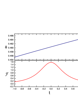
Figure 8: (Colored online) The solution for the coupling function ${\cal F}(t)$ and the imposed Galileon field $\phi(t)$, under the imposed bouncing ansatz (69). We choose the parameters as $g=1$, $V_{0}=1/12$, $c=2\sqrt{3}$, $\omega=1$, $\phi_{I}=0.1$, $t_{I}=-100$, and $t_{B\pm}=\pm 1$.

Figure 9: (Colored online) The reconstructed coupling function ${\cal F}(\phi)$ under the imposed bouncing ansatz (69), using Fig. 8. We choose the parameters as $g=1$, $V_{0}=1/12$, $c=2\sqrt{3}$, $\omega=1$, $\phi_{I}=0.1$, $t_{I}=-100$, and $t_{B\pm}=\pm 1$.

For the field $\phi$ and the potential $V(\phi)$, enlightened by the analysis of subsection III.1 and without loss of generality, respectively we assume

$$\phi(t)=\phi_{I}\ln(t-t_{I})~{}$$ (71)

and

$$V(\phi)=-V_{0}e^{c\phi}~{},$$ (72)

while as we mentioned we set $W(\sigma)=0$.

We follow the procedure described above, and for the model parameters we choose $g=1$, $V_{0}=1/12$, $c=2\sqrt{3}$, $\omega=1$, $\phi_{I}=0.1$, $t_{I}=-100$, and $t_{B\pm}=\pm 1$. In Fig. 8 we depict the solution for ${\cal F}(t)$ and also the known $\phi(t)$ from (71), and in Fig. 9 we present the corresponding reconstructed ${\cal F}(\phi)$. Finally, for completeness in Fig. 10 we show the solution for $\sigma(t)$.

Figure 10: (Colored online) The solution for the curvaton field $\sigma(t)$, under the imposed bouncing ansatz (69). We choose the parameters as $g=1$, $V_{0}=1/12$, $c=2\sqrt{3}$, $\omega=1$, $\phi_{I}=0.1$, $t_{I}=-100$, and $t_{B\pm}=\pm 1$.

We close this section by mentioning that in principle one could think of other reconstructing procedures, for instance setting ${\cal F}(\phi)$ and reconstruct ${\cal G}(\phi)$ and $W(\sigma)$, or even setting $\phi(t)$ and $\sigma(t)$ and reconstruct ${\cal F}(\phi)$, ${\cal G}(\phi)$ and $W(\sigma)$. So there can actually be many possibilities to realize the non-singular bounce.

VI Conclusions

Bounce cosmology is an interesting paradigm since it alleviates the Big-Bang singularity problem. Additionally, it can solve the Big-Bang problems, and nearly scale-invariant primordial perturbations can be incorporated too. These features make bouncing cosmologies successful alternatives to inflation. However, there are many detailed issues that should be carefully addressed during the establishment of bouncing cosmology, and in the present work we tried to confront some of them.

First of all, the NEC violation, which is required for the bounce realization, may bring ghost degrees of freedom. In the above analysis we were based on the Galileon scenario, which is a higher-derivative construction free of ghosts, and thus we obtained a bouncing evolution free of ghost and gradient instabilities.

However, there is a second problem that may disturb the bounce construction, namely that in the contracting phase even a tiny anisotropic fluctuation from the totally isotropic FRW geometry will be radically enhanced and destroy completely the FRW evolution. The solution of this “anisotropy problem” requires the total EoS of the universe to lie in the regime $w>1$ in the contracting phase. Thus, starting from Qiu:2011cy where the anisotropy problem was present, in this work we were able to solve it and obtain $w>1$ by considering an Ekpyrotic-like potential with negative value. This is one of the main contributions of the present article.

The above solution of the anisotropy problem through a large EoS has an undesired effect, namely it spoils the generation of a nearly scale-invariant power spectrum, that a scalar with smaller EoS can bring through adiabatic perturbation. Therefore, in order to still be able to produce a power spectrum in agreement with observations, we additionally introduced in the scenario a second, curvaton field, coupled to the Galileon one, which can indeed generate the desired perturbations in an isocurvature way. In our analysis we presented this mechanism in general, and we analyzed explicitly two specific examples where nearly scale-invariant perturbations are generated. Finally, we examined the conditions under which the curvaton field does not cause a significant backreaction on the background bouncing behavior caused by the Galileon field.

Furthermore, the curvaton field, apart from the generation of the desired perturbations, has another important role, namely after the bounce it can regularize the background evolution in order to avoid a Big-Rip singularity, which is caused by the Galileon field itself. In particular, although the curvaton backreaction is not significant at the background level before the bounce, during and after the bounce it becomes important and changes the background evolution. In order to see this effect we performed a semi-analytically “inverse” analysis, reconstructing suitably the desired bouncing evolution of the scale factor, which is free of a Big-Rip without any fine-tuning. We mention here that since the region where the scale-invariant spectrum is generated lies in the contracting phase, while the region where the Big-Bang is avoided is around and after the bounce point, the conditions on the functions that generate scale-invariance perturbations should hold in the contracting phase while those for the Big-Bang avoidance should hold around and after the bounce. Therefore, one can always match the required function form of the contracting regime with the required form of the bounce regime, to obtain both perturbation scale invariance and Big-Bang avoidance, although not always analytically.

We close this work by mentioning that there could be other possibilities to avoid the Big-Rip singularity. For instance, an alternative evolution after the bounce would be to assume that the Galileon and curvaton fields decay to standard model particles Langlois:2013dh . In this case the decaying Galileon energy density cannot trigger the Big Rip anymore, and additionally it can produce the matter content of the universe. Such a detailed analysis of the post-bounce evolution, and its relation to the subsequent thermal history of the universe, lies beyond the scope of the present work and it is left for a future investigation.

Note added: After completing our manuscript, we came to know that studies of bounce cosmology aiming to the same issue has been done in Osipov:2013ssa , in which similar results are obtained for different (conformal) Galileon models but with the same (Ekpyrotic-like) potential.

- (1) M. Novello and S. E. P. Bergliaffa, Phys. Rept. 463, 127 (2008) [arXiv:0802.1634 [astro-ph]].
- (2) Y. -F. Cai, T. Qiu, R. Brandenberger, Y. -S. Piao and X. Zhang, JCAP 0803, 013 (2008) [arXiv:0711.2187 [hep-th]]; Y. -F. Cai, T. -t. Qiu, J. -Q. Xia and X. Zhang, Phys. Rev. D 79, 021303 (2009) [arXiv:0808.0819 [astro-ph]]; Y. -F. Cai, T. -t. Qiu, R. Brandenberger and X. -m. Zhang, Phys. Rev. D 80, 023511 (2009) [arXiv:0810.4677 [hep-th]].
- (3) Y. -F. Cai and X. Zhang, JCAP 0906, 003 (2009) [arXiv:0808.2551 [astro-ph]]; Y. -F. Cai, W. Xue, R. Brandenberger and X. Zhang, JCAP 0905, 011 (2009) [arXiv:0903.0631 [astro-ph.CO]]; Y. -F. Cai, W. Xue, R. Brandenberger and X. -m. Zhang, JCAP 0906, 037 (2009) [arXiv:0903.4938 [hep-th]].
- (4) T. Qiu and K. -C. Yang, JCAP 1011, 012 (2010) [arXiv:1007.2571 [astro-ph.CO]].
- (5) Y. -F. Cai, T. Qiu, Y. -S. Piao, M. Li and X. Zhang, JHEP 0710, 071 (2007) [arXiv:0704.1090 [gr-qc]].
- (6) Y. -F. Cai, E. N. Saridakis, M. R. Setare and J. -Q. Xia, Phys. Rept. 493, 1 (2010) [arXiv:0909.2776 [hep-th]].
- (7) Y. -F. Cai and E. N. Saridakis, J. Cosmol. 17, 7238 (2011) [arXiv:1108.6052 [gr-qc]]; S. ’i. Nojiri and E. N. Saridakis, arXiv:1301.2686 [hep-th].
- (8) S. M. Carroll, M. Hoffman and M. Trodden, Phys. Rev. D 68, 023509 (2003) [astro-ph/0301273].
- (9) J. M. Cline, S. Jeon and G. D. Moore, Phys. Rev. D 70, 043543 (2004) [hep-ph/0311312].
- (10) S. Capozziello and M. De Laurentis, Phys. Rept. 509, 167 (2011) [arXiv:1108.6266 [gr-qc]].
- (11) T. Biswas, A. Mazumdar and W. Siegel, JCAP 0603, 009 (2006) [hep-th/0508194]; T. Biswas, T. Koivisto and A. Mazumdar, JCAP 1011, 008 (2010) [arXiv:1005.0590 [hep-th]]; T. Biswas, E. Gerwick, T. Koivisto and A. Mazumdar, Phys. Rev. Lett. 108, 031101 (2012) [arXiv:1110.5249 [gr-qc]]; T. Biswas, A. S. Koshelev, A. Mazumdar and S. Y. .Vernov, JCAP 1208, 024 (2012) [arXiv:1206.6374 [astro-ph.CO]].
- (12) C. L. Bennett, D. Larson, J. L. Weiland, N. Jarosik, G. Hinshaw, N. Odegard, K. M. Smith and R. S. Hill et al., arXiv:1212.5225 [astro-ph.CO]; G. Hinshaw, D. Larson, E. Komatsu, D. N. Spergel, C. L. Bennett, J. Dunkley, M. R. Nolta and M. Halpern et al., arXiv:1212.5226 [astro-ph.CO].
- (13) Y. -S. Piao and Y. -Z. Zhang, Phys. Rev. D 70, 043516 (2004) [astro-ph/0403671]; Y. -S. Piao, Phys. Lett. B 606, 245 (2005) [hep-th/0404002].
- (14) T. Qiu, JCAP 1206, 041 (2012) [arXiv:1204.0189 [hep-ph]]; T. Qiu, Phys. Lett. B 718, 475 (2012) [arXiv:1208.4759 [astro-ph.CO]].
- (15) F. Finelli and R. Brandenberger, Phys. Rev. D 65, 103522 (2002) [hep-th/0112249].
- (16) K. E. Kunze and R. Durrer, Class. Quant. Grav. 17, 2597 (2000) [arXiv:gr-qc/9912081]; J. K. Erickson, D. H. Wesley, P. J. Steinhardt and N. Turok, Phys. Rev. D 69, 063514 (2004) [arXiv:hep-th/0312009]; B. Xue and P. J. Steinhardt, Phys. Rev. Lett. 105, 261301 (2010) [arXiv:1007.2875 [hep-th]]; B. Xue and P. J. Steinhardt, Phys. Rev. D 84, 083520 (2011) [arXiv:1106.1416 [hep-th]].
- (17) J. Karouby and R. Brandenberger, Phys. Rev. D 82, 063532 (2010) [arXiv:1004.4947 [hep-th]]; J. Karouby, T. Qiu and R. Brandenberger, Phys. Rev. D 84, 043505 (2011) [arXiv:1104.3193 [hep-th]].
- (18) J. Khoury and P. J. Steinhardt, Phys. Rev. Lett. 104, 091301 (2010) [arXiv:0910.2230 [hep-th]]; A. Linde, V. Mukhanov and A. Vikman, JCAP 1002, 006 (2010) [arXiv:0912.0944 [hep-th]]; J. Khoury and P. J. Steinhardt, Phys. Rev. D 83, 123502 (2011) [arXiv:1101.3548 [hep-th]].
- (19) J. Khoury, B. A. Ovrut, P. J. Steinhardt and N. Turok, Phys. Rev. D 64, 123522 (2001) [arXiv:hep-th/0103239]; J. Khoury, B. A. Ovrut, N. Seiberg, P. J. Steinhardt and N. Turok, Phys. Rev. D 65, 086007 (2002) [arXiv:hep-th/0108187]; J. Khoury, B. A. Ovrut, P. J. Steinhardt and N. Turok, Phys. Rev. D 66, 046005 (2002) [arXiv:hep-th/0109050].
- (20) F. Finelli, Phys. Lett. B 545, 1 (2002) [hep-th/0206112]; A. Notari and A. Riotto, Nucl. Phys. B 644, 371 (2002) [hep-th/0205019]; K. Koyama and D. Wands, JCAP 0704, 008 (2007) [hep-th/0703040 [HEP-TH]]; K. Koyama, S. Mizuno and D. Wands, Class. Quant. Grav. 24, 3919 (2007) [arXiv:0704.1152 [hep-th]].
- (21) J. -L. Lehners, P. McFadden, N. Turok and P. J. Steinhardt, Phys. Rev. D 76, 103501 (2007) [hep-th/0702153 [HEP-TH]].
- (22) E. I. Buchbinder, J. Khoury and B. A. Ovrut, Phys. Rev. D 76, 123503 (2007) [hep-th/0702154].
- (23) J. -L. Lehners and P. J. Steinhardt, Phys. Rev. D 77, 063533 (2008) [arXiv:0712.3779 [hep-th]].
- (24) K. Hinterbichler and J. Khoury, JCAP 1204, 023 (2012) [arXiv:1106.1428 [hep-th]]; M. Libanov, S. Mironov and V. Rubakov, Phys. Rev. D 84, 083502 (2011) [arXiv:1105.6230 [astro-ph.CO]]; P. Creminelli, Phys. Rev. D 85, 041302 (2012) [arXiv:1108.0874 [hep-th]].
- (25) I. Y. .Aref’eva, N. V. Bulatov, L. V. Joukovskaya and S. Y. .Vernov, Phys. Rev. D 80, 083532 (2009) [arXiv:0903.5264 [hep-th]]; E. Elizalde, E. O. Pozdeeva and S. Y. .Vernov, Phys. Rev. D 85, 044002 (2012) [arXiv:1110.5806 [astro-ph.CO]].
- (26) A. Nicolis, R. Rattazzi and E. Trincherini, Phys. Rev. D 79, 064036 (2009) [arXiv:0811.2197 [hep-th]]; C. Deffayet, G. Esposito-Farese and A. Vikman, Phys. Rev. D 79, 084003 (2009) [arXiv:0901.1314 [hep-th]]; A. Nicolis, R. Rattazzi and E. Trincherini, JHEP 1005, 095 (2010) [Erratum-ibid. 1111, 128 (2011)] [arXiv:0912.4258 [hep-th]].
- (27) C. Deffayet, S. Deser and G. Esposito-Farese, Phys. Rev. D 80, 064015 (2009) [arXiv:0906.1967 [gr-qc]]; C. Deffayet, X. Gao, D. A. Steer and G. Zahariade, Phys. Rev. D 84, 064039 (2011) [arXiv:1103.3260 [hep-th]].
- (28) F. P. Silva and K. Koyama, Phys. Rev. D 80, 121301 (2009) [arXiv:0909.4538 [astro-ph.CO]]; P. Creminelli, A. Nicolis and E. Trincherini, JCAP 1011, 021 (2010) [arXiv:1007.0027 [hep-th]]; C. Deffayet, S. Deser and G. Esposito-Farese, Phys. Rev. D 82, 061501 (2010) [arXiv:1007.5278 [gr-qc]]; C. Deffayet, O. Pujolas, I. Sawicki and A. Vikman, JCAP 1010, 026 (2010) [arXiv:1008.0048 [hep-th]]; T. Kobayashi, M. Yamaguchi and J. ’i. Yokoyama, Phys. Rev. Lett. 105, 231302 (2010) [arXiv:1008.0603 [hep-th]]; L. Levasseur Perreault, R. Brandenberger and A. -C. Davis, Phys. Rev. D 84, 103512 (2011) [arXiv:1105.5649 [astro-ph.CO]]; Z. G. Liu, J. Zhang and Y. S. Piao, Phys. Rev. D 84, 063508 (2011), arXiv:1105.5713 [astro-ph.CO]; T. Kobayashi, M. Yamaguchi and J. ’i. Yokoyama, Prog. Theor. Phys. 126, 511 (2011) [arXiv:1105.5723 [hep-th]]; J. Evslin, T. Qiu, JHEP 1111, 032 (2011) [arXiv:1106.0570 [hep-th]]; X. Gao and D. A. Steer, JCAP 1112, 019 (2011) [arXiv:1107.2642 [astro-ph.CO]]; X. Gao, T. Kobayashi, M. Yamaguchi and J. ’i. Yokoyama, Phys. Rev. Lett. 107, 211301 (2011) [arXiv:1108.3513 [astro-ph.CO]]; H. Wang, T. Qiu and Y. -S. Piao, Phys. Lett. B 707, 11 (2012) [arXiv:1110.1795 [hep-ph]]; M. Li, T. Qiu, Y. Cai and X. Zhang, JCAP 1204, 003 (2012) [arXiv:1112.4255 [hep-th]]; X. Gao, T. Kobayashi, M. Shiraishi, M. Yamaguchi, J. ’i. Yokoyama and S. Yokoyama, arXiv:1207.0588 [astro-ph.CO]; Z. -G. Liu and Y. -S. Piao, Phys. Lett. B 718, 734 (2013) [arXiv:1207.2568 [gr-qc]]; G. Leon and E. N. Saridakis, JCAP 1303, 025 (2013) [arXiv:1211.3088 [astro-ph.CO]].
- (29) A. De Felice and S. Tsujikawa, JCAP 1202, 007 (2012) [arXiv:1110.3878 [gr-qc]].
- (30) G. W. Horndeski, Int. J. Theor. Phys. 10, 363 (1974).
- (31) T. Qiu, J. Evslin, Y. -F. Cai, M. Li and X. Zhang, JCAP 1110, 036 (2011) [arXiv:1108.0593 [hep-th]].
- (32) D. A. Easson, I. Sawicki and A. Vikman, JCAP 1111, 021 (2011) [arXiv:1109.1047 [hep-th]].
- (33) Y. -F. Cai, D. A. Easson and R. Brandenberger, JCAP 1208, 020 (2012) [arXiv:1206.2382 [hep-th]].
- (34) Y. -F. Cai, R. Brandenberger and P. Peter, arXiv:1301.4703 [gr-qc].
- (35) C. Lin, R. H. Brandenberger and L. Levasseur Perreault, JCAP 1104, 019 (2011) [arXiv:1007.2654 [hep-th]].
- (36) Y. -F. Cai and E. N. Saridakis, JCAP 0910, 020 (2009) [arXiv:0906.1789 [hep-th]]; Y. -F. Cai and E. N. Saridakis, Class. Quant. Grav. 28, 035010 (2011) [arXiv:1007.3204 [astro-ph.CO]]; Y. -F. Cai, S. -H. Chen, J. B. Dent, S. Dutta and E. N. Saridakis, Class. Quant. Grav. 28, 215011 (2011) [arXiv:1104.4349 [astro-ph.CO]]; Y. -F. Cai, C. Gao and E. N. Saridakis, JCAP 1210, 048 (2012) [arXiv:1207.3786 [astro-ph.CO]].
- (37) C. W. Misner, K. S. Thorne and J. A. Wheeler, Gravitation, San Francisco (1973).
- (38) J. DBarrow and K. Yamamoto, Phys. Rev. D 82, 063516 (2010) [arXiv:1004.4767 [gr-qc]].
- (39) G. N. Felder, A. V. Frolov, L. Kofman and A. D. Linde, Phys. Rev. D 66, 023507 (2002) [hep-th/0202017]; J. E. Lidsey and D. J. Mulryne, Phys. Rev. D 73, 083508 (2006) [hep-th/0601203]; T. Biswas, T. Koivisto and A. Mazumdar, arXiv:1105.2636 [astro-ph.CO].
- (40) R. L. Arnowitt, S. Deser and C. W. Misner, arXiv:gr-qc/0405109.
- (41) D. H. Lyth and D. Wands, Phys. Lett. B 524, 5 (2002) [arXiv:hep-ph/0110002]; D. H. Lyth, C. Ungarelli and D. Wands, Phys. Rev. D 67, 023503 (2003) [arXiv:astro-ph/0208055].
- (42) N. Deruelle and V. F. Mukhanov, Phys. Rev. D 52, 5549 (1995) [gr-qc/9503050].
- (43) D. Langlois and T. Takahashi, arXiv:1301.3319 [astro-ph.CO]; H. Assadullahi, H. Firouzjahi, M. H. Namjoo and D. Wands, arXiv:1301.3439 [hep-th].
- (44) M. Osipov and V. Rubakov, arXiv:1303.1221 [hep-th].