Supersymmetric Descendants of Self-Adjointly Extended Quantum Mechanical Hamiltonians

Abstract

We consider the descendants of self-adjointly extended Hamiltonians in supersymmetric quantum mechanics on a half-line, on an interval, and on a punctured line or interval. While there is a 4-parameter family of self-adjointly extended Hamiltonians on a punctured line, only a 3-parameter sub-family has supersymmetric descendants that are themselves self-adjoint. We also address the self-adjointness of an operator related to the supercharge, and point out that only a sub-class of its most general self-adjoint extensions is physical. Besides a general characterization of self-adjoint extensions and their supersymmetric descendants, we explicitly consider concrete examples, including a particle in a box with general boundary conditions, with and without an additional point interaction. We also discuss bulk-boundary resonances and their manifestation in the supersymmetric descendant.

1 Introduction

The differences between Hermiticity and self-adjointness of quantum mechanical operators [1] were first understood by von Neumann [2], but are rarely emphasized in the quantum mechanics textbook literature. Even standard textbook problems such as a particle confined to a box [3] or endowed with a point interaction [4, 5, 6, 7] become much richer when studied systematically in the context of self-adjointly extended Hamiltonians [8]. Self-adjoint extensions arise naturally at spatial boundaries, such as the interfaces in semiconductor heterostructures including quantum dots, quantum wires, and quantum wells [9], or at singular points, e.g. at the location of a cosmic string or vortex, which may manifest themselves as the tip of a cone in $(2+1)$ space-time dimensions [10, 11, 12, 13]. At a spatial boundary, a real-valued self-adjoint extension parameter characterizes the so-called Robin boundary conditions, which interpolate between Dirichlet and Neumann boundary conditions [14, 15, 16, 17, 18, 19]. Robin boundary conditions have also been used in quantum field theory, for example, in investigations of the Casimir effect [20, 21] and of the AdS/CFT correspondence [22]. The confinement of atoms or molecules in a finite region of space is an important subject in nanotechnology [23]. Recently, we have derived a generalized Heisenberg uncertainty relation for a quantum dot with general Robin boundary conditions [8]. As special cases, we have investigated electrons in a spherical cavity bound to its center by harmonic [24] or Coulomb forces [25], with a focus on the resulting accidental symmetries [26, 27]. General Robin boundary conditions may lead to bound states localized on the confining wall. In these cases, we have encountered bulk-boundary resonances whose wave functions are partly localized near the boundary and partly near the center of the cavity.

Supersymmetric quantum mechanics has deepened the understanding of quantum mechanics by associating a chain of supersymmetric descendants to a given quantum mechanical Hamiltonian [28, 29, 30, 31]. In this way, the number of analytically solvable quantum mechanical problems has been extended significantly. General point interactions have been investigated in the framework of supersymmetric quantum mechanics in [32, 33, 34, 35, 36, 37]. Here we study the superpartners of self-adjointly extended Hamiltonians. Remarkably, these are not automatically self-adjoint. In particular, only a 3-parameter sub-family of the general 4-parameter family of self-adjointly extended Hamiltonians on a punctured line have supersymmetric descendants that are themselves self-adjoint. We also construct the self-adjoint extensions of an operator related to the supercharge. Since we consider a Hamiltonian and its supersymmetric descendant as two different physical systems, rather than as two parts of the same system, only a sub-class of self-adjoint extensions of this operator is physical.

We illustrate our general results with specific systems, including a particle confined to a box with or without an additional point interaction. We will again encounter bulk-boundary resonances, and we study their manifestation in the corresponding supersymmetric descendant. While there are experimental realizations of bulk-boundary resonances, e.g. for atoms encapsulated in fullerenes [38, 39], our current study is not motivated by a particular application. Instead, we aim at illuminating the relations between the theoretical concepts of supersymmetry and self-adjoint extensions in quantum mechanics in general.

Some of the concrete systems studied here are so simple that they could easily serve as problems in the teaching of quantum mechanics. In this sense, our paper also has pedagogical intentions, by trying to convince the reader that the theory of self-adjoint extensions is not only mathematically elegant, but also of great physical relevance, that deserves a more prominent place in the teaching of quantum mechanics.

The rest of this paper is organized as follows. In section 2 we consider the general self-adjoint extensions of quantum mechanical Hamiltonians on a half-line as well as on a punctured line, and we address the issue of self-adjointness of an operator constructed from the supercharge. In section 3, we investigate concrete examples of a particle confined to a box, or endowed with a point interaction, and we study the phenomenon of bulk-boundary resonances. Finally, section 4 contains our conclusions.

2 Self-Adjointness of Supersymmetric Descendant Hamiltonians

After briefly reviewing the basics of supersymmetric quantum mechanics [28, 29], in this section, we study the self-adjoint extensions of the Hamiltonian of a particle on a half-line and on a punctured line, and we investigate their supersymmetric descendants. In addition, we investigate the self-adjointness of an operator constructed from the supercharge.

2.1 Basics of Supersymmetric Quantum Mechanics

In order to make this paper self-contained, let us briefly review the basics of supersymmetric quantum mechanics in one spatial dimension. We consider a non-relativistic particle of mass $m$ moving under the influence of a potential $V(x)$ such that

$$-\frac{1}{2m}\partial_{x}^{2}\Psi_{n}(x)+V(x)\Psi_{n}(x)=E_{n}\Psi_{n}(x)\ \Rightarrow$$

$$-\partial_{x}^{2}\Psi_{n}(x)+2mV(x)\Psi_{n}(x)=\lambda_{n}\Psi_{n}(x),\quad\lambda_{n}=2mE_{n}.$$ (2.1)

Introducing the real-valued superpotential $W(x)$ we define

$$A=\partial_{x}+W(x),\quad A^{\dagger}=-\partial_{x}+W(x).$$ (2.2)

We construct the Hamiltonian as

$$2mH=A^{\dagger}A=[-\partial_{x}+W(x)][\partial_{x}+W(x)]=-\partial_{x}^{2}-\partial_{x}W(x)+W(x)^{2},$$ (2.3)

and thus identify the potential as

$$2mV(x)=-\partial_{x}W(x)+W(x)^{2},$$ (2.4)

such that

$$H\Psi_{n}(x)=E_{n}\Psi_{n}(x)\ \Rightarrow\ 2mH\Psi_{n}(x)=\lambda_{n}\Psi_{n}(x).$$ (2.5)

Shifting the potential such that the ground state energy vanishes, i.e. $\lambda_{0}=0$, one obtains

$$H\Psi_{0}(x)=0\ \Rightarrow\ A\Psi_{0}(x)=[\partial_{x}+W(x)]\Psi_{0}(x)=0,$$ (2.6)

which allows us to relate the superpotential to the ground state wave function

$$W(x)=-\frac{\partial_{x}\Psi_{0}(x)}{\Psi_{0}(x)}=-\partial_{x}\log\Psi_{0}(x).$$ (2.7)

We now define the supersymmetric descendant Hamiltonian as

$$2mH^{\prime}=AA^{\dagger}=[\partial_{x}+W(x)][-\partial_{x}+W(x)]=-\partial_{x}^{2}+\partial_{x}W(x)+W(x)^{2},$$ (2.8)

with the potential

$$2mV^{\prime}(x)=\partial_{x}W(x)+W(x)^{2}.$$ (2.9)

The eigenstates of $H^{\prime}$ are related to the eigenstates of $H$ by

$$\Psi_{n}^{\prime}(x)=\frac{1}{\sqrt{\lambda_{n}}}A\Psi_{n}(x),\ n>0,$$ (2.10)

such that indeed

$$2mH^{\prime}\Psi_{n}^{\prime}(x)=\frac{1}{\sqrt{\lambda_{n}}}AA^{\dagger}A\Psi_{n}(x)=\sqrt{\lambda_{n}}A\Psi_{n}(x)=\lambda_{n}\Psi_{n}^{\prime}(x).$$ (2.11)

Hence, the spectrum of $H^{\prime}$ coincides with the spectrum of excited states of $H$. The normalization of the superpartner wave functions is given by

$$\langle\Psi_{n}^{\prime}|\Psi_{n}^{\prime}\rangle=\frac{1}{\lambda_{n}}\langle\Psi_{n}|A^{\dagger}A|\Psi_{n}\rangle=1.$$ (2.12)

It should be noted that eq.(2.10) works even for the continuous part of the spectrum, when the wave functions are not normalizable in the usual sense. If the wave function

$$\Psi_{0}(x)=C\exp\left(-\int_{0}^{x}dx^{\prime}\ W(x^{\prime})\right)$$ (2.13)

is not square-integrable, $H$ does not have a normalizable ground state of zero energy. In that case, the spectra of $H$ and $H^{\prime}$ are completely identical and supersymmetry is spontaneously broken. In this paper we will only encounter unbroken supersymmetry.

By applying the same procedure again, one obtains the next superpotential

$$W^{\prime}(x)=-\frac{\partial_{x}\Psi_{1}^{\prime}(x)}{\Psi_{1}^{\prime}(x)},$$ (2.14)

such that

$$2mV^{\prime}(x)-\lambda_{1}=-\partial_{x}W^{\prime}(x)+W^{\prime}(x)^{2},$$

$$2mV^{\prime\prime}(x)-\lambda_{1}=\partial_{x}W^{\prime}(x)+W^{\prime}(x)^{2}.$$ (2.15)

By iterating the construction, as long as the system has a discrete spectrum of bound states, one can then generate a chain of supersymmetric descendants.

Let us also consider the supercharge and its Hermitean conjugate

$${\cal Q}=\left(\begin{array}[]{cc}0&0\\ A&0\end{array}\right),\quad{\cal Q}^{\dagger}=\left(\begin{array}[]{cc}0&A^{\dagger}\\ 0&0\end{array}\right),$$ (2.16)

which generate the Hamiltonians $H$ and $H^{\prime}$ by anti-commutation

$$\{{\cal Q},{\cal Q}^{\dagger}\} = \left(\begin{array}[]{cc}0&0\\ A&0\end{array}\right)\left(\begin{array}[]{cc}0&A^{\dagger}\\ 0&0\end{array}\right)+\left(\begin{array}[]{cc}0&A^{\dagger}\\ 0&0\end{array}\right)\left(\begin{array}[]{cc}0&0\\ A&0\end{array}\right)$$ (2.25)

$$= \left(\begin{array}[]{cc}A^{\dagger}A&0\\ 0&AA^{\dagger}\end{array}\right)=\left(\begin{array}[]{cc}H&0\\ 0&H^{\prime}\end{array}\right)={\cal H}.$$ (2.30)

The supercharge is nilpotent and commutes with the Hamiltonian, i.e.

$${\cal Q}^{2}={{\cal Q}^{\dagger}}^{2}=0,\quad[{\cal Q},{\cal H}]=[{\cal Q}^{\dagger},{\cal H}]=0.$$ (2.31)

While the supercharge itself is not Hermitean, it is natural to construct the operator

$${\cal Q}_{+}={\cal Q}+{\cal Q}^{\dagger}=\left(\begin{array}[]{cc}0&A^{\dagger}\\ A&0\end{array}\right),$$ (2.32)

which yields ${\cal Q}_{+}^{2}={\cal H}$, and is “Hermitean” at a rather formal level. Later, we’ll properly address the self-adjointness of ${\cal Q}_{+}$ [37].

2.2 Particle on a Half-Line

Let us consider a particle confined to a half-line, the region $x\leq x_{0}$. If the region $x>x_{0}$ is energetically forbidden, the standard textbook approach is to demand Dirichlet boundary conditions, i.e. $\Psi(x_{0})=0$. However, this is not really necessary. It suffices that the probability current density,

$$j(x)=\frac{1}{2mi}\left[\Psi(x)^{*}\partial_{x}\Psi(x)-\partial_{x}\Psi(x)^{*}\Psi(x)\right],$$ (2.33)

vanishes at the boundary, i.e. $j(x)=0$. This is the case, not only for the Dirichlet boundary condition, but also for the more general Robin boundary condition

$$\partial_{x}\Psi(x_{0})+\gamma\Psi(x_{0})=0,$$ (2.34)

which yields

$$j(x_{0})=\frac{1}{2mi}\left[\Psi(x_{0})^{*}\partial_{x}\Psi(x_{0})-\partial_{x}\Psi(x_{0})^{*}\Psi(x_{0})\right]=\frac{1}{2mi}\Psi(x_{0})^{*}\Psi(x_{0})(\gamma^{*}-\gamma).$$ (2.35)

This indeed vanishes, provided that $\gamma\in{\mathbb{R}}$.

In order to investigate whether the Hamiltonian, endowed with the Robin boundary condition eq.(2.34), is indeed self-adjoint, let us consider

$$\langle\chi|2mH|\Psi\rangle = \int_{-\infty}^{x_{0}}dx\ \chi(x)^{*}[-\partial_{x}^{2}+2mV(x)]\Psi(x)$$ (2.36)

$$= \int_{-\infty}^{x_{0}}dx\ [\partial_{x}\chi(x)^{*}\partial_{x}\Psi(x)+\chi(x)^{*}2mV(x)\Psi(x)]-\left[\chi(x)^{*}\partial_{x}\Psi(x)\right]_{-\infty}^{x_{0}}$$

$$= \int_{-\infty}^{x_{0}}dx\ \Psi(x)[-\partial_{x}^{2}+2mV(x)]\chi(x)^{*}$$

$$+ \left[\partial_{x}\chi(x)^{*}\Psi(x)-\chi(x)^{*}\partial_{x}\Psi(x)\right]_{-\infty}^{x_{0}}$$

$$= \langle\Psi|2mH|\chi\rangle^{*}+\left[\partial_{x}\chi(x)^{*}\Psi(x)-\chi(x)^{*}\partial_{x}\Psi(x)\right]_{-\infty}^{x_{0}}.$$

The Hamiltonian is Hermitean (or symmetric in mathematical parlance) if

$$\langle\chi|H|\Psi\rangle=\langle H^{\dagger}\chi|\Psi\rangle=\langle H\chi|\Psi\rangle=\langle\Psi|H|\chi\rangle^{*}.$$ (2.37)

This is the case, only if

$$\left[\partial_{x}\chi(x)^{*}\Psi(x)-\chi(x)^{*}\partial_{x}\Psi(x)\right]_{-\infty}^{x_{0}}=0.$$ (2.38)

Assuming that the wave functions are normalizable and thus vanish at infinity, we thus conclude that Hermiticity of $H$ requires

$$\partial_{x}\chi(x_{0})^{*}\Psi(x_{0})-\chi(x_{0})^{*}\partial_{x}\Psi(x_{0})=0.$$ (2.39)

Here we have also assumed that the potential $V(x)$ is not singular, such that all subtleties related to Hermiticity and self-adjointness are associated entirely with the behavior at the point $x_{0}$. The domain $D(H)$ of the Hamiltonian contains the at least twice-differentiable square-integrable wave functions $\Psi(x)$ that obey the Robin boundary condition eq.(2.34). Using that condition, eq.(2.39) reduces to

$$\Psi(x_{0})\left[\partial_{x}\chi(x_{0})^{*}+\gamma\chi(x_{0})^{*}\right]=0.$$ (2.40)

Since $\Psi(x_{0})$ need not vanish, the Hamiltonian is Hermitean if

$$\gamma^{*}\chi(x_{0})+\partial_{x}\chi(x_{0})=0.$$ (2.41)

Because $\gamma\in{\mathbb{R}}$, the wave function $\chi(x)$ must also obey the Robin boundary condition eq.(2.34). Imposing this boundary condition on $\chi(x)$ implies that the domain of $H^{\dagger}$ coincides with the domain of $H$, $D(H^{\dagger})=D(H)$. Since $H$ is indeed Hermitean when both $\Psi(x)$ and $\chi(x)$ obey eq.(2.34), and since, in addition, $D(H^{\dagger})=D(H)$, the Hamiltonian is, in fact, self-adjoint. The parameter $\gamma$ thus characterizes a 1-parameter family of self-adjoint extensions of the Hamiltonian on the half-line.

Let us now consider the boundary condition of the corresponding supersymmetric partner Hamiltonian $H^{\prime}$. The Robin boundary condition eq.(2.34) determines the value of the superpotential at the boundary

$$W(x_{0})=-\frac{\partial_{x}\Psi(x_{0})}{\Psi(x_{0})}=\gamma.$$ (2.42)

The eigenfunctions of the supersymmetric partner Hamiltonian $H^{\prime}$ then satisfy

$$\Psi_{n}^{\prime}(x_{0})=\frac{1}{\sqrt{\lambda_{n}}}[\partial_{x}+W(x_{0})]\Psi_{n}(x_{0})=\frac{1}{\sqrt{\lambda_{n}}}[\partial_{x}\Psi_{n}(x_{0})+\gamma\Psi_{n}(x_{0})]=0,$$ (2.43)

i.e. they obey the standard Dirichlet boundary condition, $\Psi_{n}^{\prime}(x_{0})=0$, which corresponds to the self-adjoint extension parameter $\gamma^{\prime}=\infty$. In this way, non-trivial information encoded in the boundary parameter $\gamma$ of the original problem, is encoded in the value of the superpotential in the supersymmetric partner problem. In particular, all supersymmetric descendants automatically obey the standard Dirichlet boundary condition.

2.3 Particle on a Punctured Line

Let us now consider a particle on a punctured line ${\mathbb{R}}\setminus\{x_{0}\}$, from which the single point $x_{0}$ has been removed. This divides the $x$-axis into two separate regions $\rm I$ with $x>x_{0}$ and $\rm II$ with $x<x_{0}$. Accordingly, we denote the wave function and the superpotential on the two sides of the puncture by

$$\Psi_{\rm I}=\Psi(x_{0}+\varepsilon),\quad\Psi_{\rm II}=\Psi(x_{0}-\varepsilon),\quad W_{\rm I}=W(x_{0}+\varepsilon),\quad W_{\rm II}=W(x_{0}-\varepsilon),\quad\varepsilon\searrow 0.$$ (2.44)

The most general boundary condition that leads to a self-adjoint Hamiltonian is then given by

$$\left(\begin{array}[]{c}\Psi_{\rm I}\\ \partial_{x}\Psi_{\rm I}\end{array}\right)=\exp(i\theta)\left(\begin{array}[]{cc}a&b\\ c&d\end{array}\right)\left(\begin{array}[]{c}\Psi_{\rm II}\\ \partial_{x}\Psi_{\rm II}\end{array}\right),\ a,b,c,d\in{\mathbb{R}},\ ad-bc=1,\ \theta\in]-\frac{\pi}{2},\frac{\pi}{2}].$$ (2.45)

The five parameters $a,b,c,d,\theta$, with the constraint $ad-bc=1$, define a 4-parameter family of self-adjoint extensions. The boundary condition (2.45) guarantees that the probability current is continuous at $x=x_{0}$, i.e.

$$2mi\ j_{\rm I}\!\! = \!\!\Psi_{\rm I}^{*}\partial_{x}\Psi_{\rm I}-\partial_{x}\Psi_{\rm I}^{*}\Psi_{\rm I}=(\Psi_{\rm I}^{*},\partial_{x}\Psi_{\rm I}^{*})\left(\begin{array}[]{cc}0&1\\ -1&0\end{array}\right)\left(\begin{array}[]{c}\Psi_{\rm I}\\ \partial_{x}\Psi_{\rm I}\end{array}\right)$$ (2.50)

$$= \!\!(\Psi_{\rm II}^{*},\partial_{x}\Psi_{\rm II}^{*})\exp(-i\theta)\left(\begin{array}[]{cc}a&c\\ b&d\end{array}\right)\left(\begin{array}[]{cc}0&1\\ -1&0\end{array}\right)\exp(i\theta)\left(\begin{array}[]{cc}a&b\\ c&d\end{array}\right)\left(\begin{array}[]{c}\Psi_{\rm II}\\ \partial_{x}\Psi_{\rm II}\end{array}\right)$$ (2.59)

$$= \!\!(\Psi_{\rm II}^{*},\partial_{x}\Psi_{\rm II}^{*})\left(\begin{array}[]{cc}0&1\\ -1&0\end{array}\right)\left(\begin{array}[]{c}\Psi_{\rm II}\\ \partial_{x}\Psi_{\rm II}\end{array}\right)=2mi\ j_{\rm II}.$$ (2.64)

In this case, the Hermiticity of the Hamiltonian requires

$$\partial_{x}\chi_{\rm I}^{*}\Psi_{\rm I}-\chi_{\rm I}^{*}\partial_{x}\Psi_{\rm I}=\partial_{x}\chi_{\rm II}^{*}\Psi_{\rm II}-\chi_{\rm II}^{*}\partial_{x}\Psi_{\rm II},$$ (2.65)

which implies

$$\Psi_{\rm II}(\partial_{x}\chi_{\rm I}^{*}\exp(i\theta)a-\chi_{\rm I}^{*}\exp(i\theta)c-\partial_{x}\chi_{\rm II}^{*})+$$

$$\partial_{x}\Psi_{\rm II}(\partial_{x}\chi_{\rm I}^{*}\exp(i\theta)b-\chi_{\rm I}^{*}\exp(i\theta)d+\chi_{\rm II}^{*})=0.$$ (2.66)

Since both $\Psi_{\rm II}$ and $\partial_{x}\Psi_{\rm II}$ can take arbitrary values, we obtain

$$\chi_{\rm II}^{*}=\chi_{\rm I}^{*}\exp(i\theta)d-\partial_{x}\chi_{\rm I}^{*}\exp(i\theta)b,$$

$$\partial_{x}\chi_{\rm II}^{*}=-\chi_{\rm I}^{*}\exp(i\theta)c+\partial_{x}\chi_{\rm I}^{*}\exp(i\theta)a\ \Rightarrow$$

$$\left(\begin{array}[]{c}\chi_{\rm II}\\ \partial_{x}\chi_{\rm II}\end{array}\right)=\exp(-i\theta)\left(\begin{array}[]{cc}d&-b\\ -c&a\end{array}\right)\left(\begin{array}[]{c}\chi_{\rm I}\\ \partial_{x}\chi_{\rm I}\end{array}\right)\ \Rightarrow$$ (2.73)

$$\left(\begin{array}[]{c}\chi_{\rm I}\\ \partial_{x}\chi_{\rm I}\end{array}\right)=\exp(i\theta)\left(\begin{array}[]{cc}a&b\\ c&d\end{array}\right)\left(\begin{array}[]{c}\chi_{\rm II}\\ \partial_{x}\chi_{\rm II}\end{array}\right).$$ (2.80)

Hence, in order to ensure Hermiticity, $\chi(x)$ must obey the same boundary condition (2.45) as $\Psi(x)$. This ensures that the domain of $H^{\dagger}$ coincides with the domain of $H$, $D(H^{\dagger})=D(H)$, which implies that $H$ is not only Hermitean, but actually self-adjoint.

2.4 Parity Symmetry

Let us investigate under what circumstances the most general self-adjoint point interaction at $x_{0}=0$ respects the parity symmetry, generated by ${}^{P}\Psi(x)=\Psi(-x)$, which implies

$${}^{P}\Psi_{\rm I}=\Psi_{\rm II},\quad^{P}\Psi_{\rm II}=\Psi_{\rm I},\quad^{P}\partial_{x}\Psi_{\rm I}=-\partial_{x}\Psi_{\rm II},\quad^{P}\partial_{x}\Psi_{\rm II}=-\partial_{x}\Psi_{\rm I}.$$ (2.81)

The point interaction is parity-symmetric if the parity partner ${}^{P}\Psi(x)$ of a wave function $\Psi(x)$ also respects the boundary condition, i.e.

$$\left(\begin{array}[]{c}^{P}\Psi_{\rm I}\\ ^{P}\partial_{x}\Psi_{\rm I}\end{array}\right)=\exp(i\theta)\left(\begin{array}[]{cc}a&b\\ c&d\end{array}\right)\left(\begin{array}[]{c}^{P}\Psi_{\rm II}\\ ^{P}\partial_{x}\Psi_{\rm II}\end{array}\right)\ \Rightarrow$$ (2.88)

$$\left(\begin{array}[]{c}\Psi_{\rm II}\\ -\partial_{x}\Psi_{\rm II}\end{array}\right)=\exp(i\theta)\left(\begin{array}[]{cc}a&b\\ c&d\end{array}\right)\left(\begin{array}[]{c}\Psi_{\rm I}\\ -\partial_{x}\Psi_{\rm I}\end{array}\right)\ \Rightarrow$$ (2.95)

$$\left(\begin{array}[]{cc}1&0\\ 0&-1\end{array}\right)\left(\begin{array}[]{c}\Psi_{\rm II}\\ \partial_{x}\Psi_{\rm II}\end{array}\right)=\exp(i\theta)\left(\begin{array}[]{cc}a&b\\ c&d\end{array}\right)\left(\begin{array}[]{cc}1&0\\ 0&-1\end{array}\right)\left(\begin{array}[]{c}\Psi_{\rm I}\\ \partial_{x}\Psi_{\rm I}\end{array}\right)\ \Rightarrow$$ (2.106)

$$\left(\begin{array}[]{c}\Psi_{\rm I}\\ \partial_{x}\Psi_{\rm I}\end{array}\right)=\exp(-i\theta)\left(\begin{array}[]{cc}1&0\\ 0&-1\end{array}\right)\left(\begin{array}[]{cc}d&-b\\ -c&a\end{array}\right)\left(\begin{array}[]{cc}1&0\\ 0&-1\end{array}\right)\left(\begin{array}[]{c}\Psi_{\rm II}\\ \partial_{x}\Psi_{\rm II}\end{array}\right)\ \Rightarrow\$$ (2.117)

$$\left(\begin{array}[]{c}\Psi_{\rm I}\\ \partial_{x}\Psi_{\rm I}\end{array}\right)=\exp(-i\theta)\left(\begin{array}[]{cc}d&b\\ c&a\end{array}\right)\left(\begin{array}[]{c}\Psi_{\rm II}\\ \partial_{x}\Psi_{\rm II}\end{array}\right).$$ (2.124)

This is consistent with the original boundary condition (2.45) only if $a=d$ and $\theta=0$.

2.5 Self-Adjointness of the Superpartner Hamiltonian

Let us now investigate the superpartner Hamiltonian $H^{\prime}$ for a particle on the punctured line, without assuming parity symmetry. First, we notice that (for $n>0$)

$$\Psi_{n}(x)=\frac{1}{\lambda_{n}}A^{\dagger}A\Psi_{n}(x)=\frac{1}{\sqrt{\lambda_{n}}}A^{\dagger}\Psi_{n}^{\prime}(x)=\frac{1}{\sqrt{\lambda_{n}}}[-\partial_{x}\Psi_{n}^{\prime}(x)+W(x)\Psi_{n}^{\prime}(x)],$$ (2.125)

such that

$$\partial_{x}\Psi_{n}^{\prime}(x) = W(x)\Psi_{n}^{\prime}(x)-\sqrt{\lambda_{n}}\Psi_{n}(x)$$ (2.126)

$$= W(x)\frac{1}{\sqrt{\lambda_{n}}}[\partial_{x}\Psi_{n}(x)+W(x)\Psi_{n}(x)]-\sqrt{\lambda_{n}}\Psi_{n}(x)$$

$$= \frac{1}{\sqrt{\lambda_{n}}}[W(x)\partial_{x}\Psi_{n}(x)+(W(x)^{2}-\lambda_{n})\Psi_{n}(x)],$$

which implies

$$\left(\begin{array}[]{c}\Psi_{n}^{\prime}(x)\\ \partial_{x}\Psi_{n}^{\prime}(x)\end{array}\right)=\frac{1}{\sqrt{\lambda_{n}}}\left(\begin{array}[]{cc}W(x)&1\\ W(x)^{2}-\lambda_{n}&W(x)\end{array}\right)\left(\begin{array}[]{c}\Psi_{n}(x)\\ \partial_{x}\Psi_{n}(x)\end{array}\right).$$ (2.127)

Based on the previous discussion, for the superpartner we again expect a boundary condition of the form

$$\left(\begin{array}[]{c}\Psi^{\prime}_{\rm I}\\ \partial_{x}\Psi^{\prime}_{\rm I}\end{array}\right)=\exp(i\theta^{\prime})\left(\begin{array}[]{cc}a^{\prime}&b^{\prime}\\ c^{\prime}&d^{\prime}\end{array}\right)\left(\begin{array}[]{c}\Psi^{\prime}_{\rm II}\\ \partial_{x}\Psi^{\prime}_{\rm II}\end{array}\right),\ a^{\prime},b^{\prime},c^{\prime},d^{\prime}\in{\mathbb{R}},\ a^{\prime}d^{\prime}-b^{\prime}c^{\prime}=1.$$ (2.128)

Using eq.(2.127), which immediately implies

$$\left(\begin{array}[]{c}\Psi_{n\rm I}^{\prime}\\ \partial_{x}\Psi_{n\rm I}^{\prime}\end{array}\right)=\frac{1}{\sqrt{\lambda_{n}}}\left(\begin{array}[]{cc}W_{\rm I}&1\\ W_{\rm I}^{2}-\lambda_{n}&W_{\rm I}\end{array}\right)\left(\begin{array}[]{c}\Psi_{n\rm I}\\ \partial_{x}\Psi_{n\rm I}\end{array}\right),$$ (2.135)

$$\left(\begin{array}[]{c}\Psi_{n\rm II}^{\prime}\\ \partial_{x}\Psi_{n\rm II}^{\prime}\end{array}\right)=\frac{1}{\sqrt{\lambda_{n}}}\left(\begin{array}[]{cc}W_{\rm II}&1\\ W_{\rm II}^{2}-\lambda_{n}&W_{\rm II}\end{array}\right)\left(\begin{array}[]{c}\Psi_{n\rm II}\\ \partial_{x}\Psi_{n\rm II}\end{array}\right),$$ (2.142)

as well as eq.(2.45), one identifies

$$\exp(i\theta^{\prime})\left(\begin{array}[]{cc}a^{\prime}&b^{\prime}\\ c^{\prime}&d^{\prime}\end{array}\right)=\left(\begin{array}[]{cc}W_{\rm I}&1\\ W_{\rm I}^{2}-\lambda_{n}&W_{\rm I}\end{array}\right)\exp(i\theta)\left(\begin{array}[]{cc}a&b\\ c&d\end{array}\right)\left(\begin{array}[]{cc}W_{\rm II}&1\\ W_{\rm II}^{2}-\lambda_{n}&W_{\rm II}\end{array}\right)^{-1}.$$ (2.143)

It is important to note that the values of the superpotential $W_{\rm I}$ and $W_{\rm II}$ at the two sides of the puncture $x_{0}$ are not independent, but are related by

$$\Psi_{0\rm I}\left(\begin{array}[]{c}1\\ -W_{\rm I}\end{array}\right) = \left(\begin{array}[]{c}\Psi_{0\rm I}\\ \partial_{x}\Psi_{0\rm I}\end{array}\right)=\exp(i\theta)\left(\begin{array}[]{cc}a&b\\ c&d\end{array}\right)\left(\begin{array}[]{c}\Psi_{0\rm II}\\ \partial_{x}\Psi_{0\rm II}\end{array}\right)$$ (2.152)

$$= \exp(i\theta)\left(\begin{array}[]{cc}a&b\\ c&d\end{array}\right)\Psi_{0\rm II}\left(\begin{array}[]{c}1\\ -W_{\rm II}\end{array}\right)=\exp(i\theta)\Psi_{0\rm II}\left(\begin{array}[]{c}a-bW_{\rm II}\\ c-dW_{\rm II}\end{array}\right),$$ (2.159)

(2.160)

such that

$$\frac{1}{-W_{\rm I}}=\frac{a-bW_{\rm II}}{c-dW_{\rm II}}\ \Rightarrow\ aW_{\rm I}-bW_{\rm I}W_{\rm II}+c-dW_{\rm II}=0,$$ (2.161)

Using this relation, it is straightforward to work out the individual matrix elements in eq.(2.143) and one obtains

$$\exp(i\theta^{\prime})a^{\prime}=\exp(i\theta)(d+bW_{\rm I}),$$

$$\exp(i\theta^{\prime})b^{\prime}=0,$$

$$\exp(i\theta^{\prime})c^{\prime}=\exp(i\theta)[(d+bW_{\rm I})W_{\rm I}-(a-bW_{\rm II})W_{\rm II}-b\lambda_{n}],$$

$$\exp(i\theta^{\prime})d^{\prime}=\exp(i\theta)(a-bW_{\rm II}).$$ (2.162)

Let us check the constraint

$$a^{\prime}d^{\prime}-b^{\prime}c^{\prime}=(d+bW_{\rm I})(a-bW_{\rm II})=ad+abW_{\rm I}-bdW_{\rm II}-b^{2}W_{\rm I}W_{\rm II}=ad-bc=1,$$ (2.163)

which is indeed correctly satisfied. Since, the parameters $a^{\prime},b^{\prime},c^{\prime},d^{\prime},\theta^{\prime}$ must be the same for every state, it is unacceptable that the eigenvalue $\lambda_{n}$ enters the expression for $c^{\prime}$ in eq.(2.5). In fact, the $\lambda_{n}$-dependence of the boundary condition implies that the superpartner Hamiltonian $H^{\prime}$ is not self-adjoint, unless $b=0$. This means that only a 3-parameter sub-family of self-adjoint Hamiltonians $H$ (namely those with $b=0$) have a self-adjoint superpartner $H^{\prime}$. In that case, the constraint $ad-bc=ad=1$ implies $d=1/a$. The self-adjoint extension parameters of the supersymmetric descendant then are

$$a^{\prime}=d=1/a,\quad b^{\prime}=0,\quad c^{\prime}=dW_{\rm I}-aW_{\rm II}=W_{\rm I}/a-aW_{\rm II},\quad d^{\prime}=a,\quad\theta^{\prime}=\theta.$$ (2.164)

For $b=0$ eq.(2.161) reduces to $c=W_{\rm II}/a-aW_{\rm I}$. It is interesting to note that $b=0$ implies that the probability density $\rho(x)=|\Psi(x)|^{2}$ (but not necessarily the wave function itself) is continuous at the puncture $x_{0}$. This is thus a necessary and sufficient condition for the self-adjointness of the superpartner. Since $b^{\prime}=0$ for the superpartner, all higher supersymmetric descendants are then also automatically self-adjoint. When the original boundary condition is parity-invariant, i.e. when $a=d=1/a=\pm 1$ and $\theta=0$, the superpartner also obeys a parity-symmetric boundary condition with

$$a^{\prime}=a=\pm 1,\quad b^{\prime}=0,\quad c^{\prime}=W_{\rm I}/a-aW_{\rm II}=-c,\quad d^{\prime}=a,\quad\theta^{\prime}=\theta=0.$$ (2.165)

Here we have used $aW_{\rm I}+bW_{\rm I}W_{\rm II}+c-dW_{\rm II}=W_{\rm I}/a-aW_{\rm II}+c=0$.

2.6 Self-Adjointness of the Operator ${\cal Q}_{+}$

Let us now investigate the self-adjoint extensions of the operator ${\cal Q}_{+}$. Introducing the 2-component wave functions

$$\widetilde{\chi}(x)=\left(\begin{array}[]{c}\chi(x)\\ \chi^{\prime}(x)\end{array}\right),\quad\widetilde{\Psi}(x)=\left(\begin{array}[]{c}\Psi(x)\\ \Psi^{\prime}(x)\end{array}\right),$$ (2.166)

for the particle on a half-line we obtain

$$\langle\widetilde{\chi}|{\cal Q}_{+}|\widetilde{\Psi}\rangle = \int_{-\infty}^{x_{0}}dx\ (\chi(x)^{*},\chi^{\prime}(x)^{*})\left(\begin{array}[]{cc}0&-\partial_{x}+W(x)\\ \partial_{x}+W(x)&0\end{array}\right)\left(\begin{array}[]{c}\Psi(x)\\ \Psi^{\prime}(x)\end{array}\right)$$

$$= \int_{-\infty}^{x_{0}}dx\ \{\chi(x)^{*}[-\partial_{x}+W(x)]\Psi^{\prime}(x)+\chi^{\prime}(x)^{*}[\partial_{x}+W(x)]\Psi(x)\}$$

$$= \int_{-\infty}^{x_{0}}dx\ \{\partial_{x}\chi(x)^{*}\Psi^{\prime}(x)+\chi(x)^{*}W(x)\Psi^{\prime}(x)$$

$$- \partial_{x}\chi^{\prime}(x)^{*}\Psi(x)+\chi^{\prime}(x)^{*}W(x)\Psi(x)\}-[\chi(x)^{*}\Psi^{\prime}(x)-\chi^{\prime}(x)^{*}\Psi(x)]_{-\infty}^{x_{0}}$$

$$= \langle\widetilde{\Psi}|{\cal Q}_{+}|\widetilde{\chi}\rangle^{*}-\chi(x_{0})^{*}\Psi^{\prime}(x_{0})+\chi^{\prime}(x_{0})^{*}\Psi(x_{0}).$$ (2.172)

Hermiticity of ${\cal Q}_{+}$ thus requires $\chi(x_{0})^{*}\Psi^{\prime}(x_{0})=\chi^{\prime}(x_{0})^{*}\Psi(x_{0})$. We make the ansatz

$$\Psi^{\prime}(x_{0})=\eta\Psi(x_{0}),$$ (2.173)

for the self-adjoint extension condition, such that Hermiticity of ${\cal Q}_{+}$ then requires

$$\chi(x_{0})^{*}\eta\Psi(x_{0})=\chi^{\prime}(x_{0})^{*}\Psi(x_{0})\ \Rightarrow\ \chi^{\prime}(x_{0})=\eta^{*}\chi(x_{0}).$$ (2.174)

Hence, the domains of ${\cal Q}_{+}$ and its adjoint ${\cal Q}_{+}^{\dagger}$ agree, i.e. $D({\cal Q}_{+})=D({\cal Q}_{+}^{\dagger})$, if and only if $\eta=\eta^{*}$, which ensures that ${\cal Q}_{+}$ is not only Hermitean but actually self-adjoint. There is a 1-parameter family of self-adjoint extensions of ${\cal Q}_{+}$ (parameterized by $\eta\in{\mathbb{R}}$).

From our previous considerations we know that $\partial_{x}\Psi(x_{0})+\gamma\Psi(x_{0})=0$ implies $\Psi^{\prime}(x_{0})=0$, which in turn leads to $\eta=0$. This seems to leave the value $\Psi(x_{0})$ unrestricted. It also seems that ${\cal Q}_{+}$ contains no free parameter, while $H$ is endowed with the Robin boundary condition characterized by $\gamma$. This apparent contradiction gets resolved when we recall that $\gamma$ is also encoded in the superpotential, i.e. $W(x_{0})=\gamma$. Hence, we may conclude that ${\cal Q}_{+}$ is indeed self-adjoint, but has a fixed extension parameter $\eta=0$. Why are we not encountering the other self-adjoint extensions of ${\cal Q}_{+}$? Actually, in our treatment of $H$ and $H^{\prime}$ those are unphysical. We should point out that we consider $H$ and its supersymmetric descendant $H^{\prime}$ as two physically distinct systems, rather than as two parts of the same system. In particular, we do not allow states with both an upper and a lower component. Consequently, probability is conserved separately for the systems associated with $H$ and $H^{\prime}$. This limits us to the self-adjoint extension of ${\cal Q}_{+}$ characterized by $\eta=0$.

Let us also consider the self-adjoint extensions of the operator ${\cal Q}_{+}$ on the punctured line, consisting of the regions $\rm I$ and $\rm II$. In that case, Hermiticity requires

$$\chi_{\rm I}^{*}\Psi^{\prime}_{\rm I}-{\chi^{\prime}_{\rm I}}^{*}\Psi_{\rm I}=\chi_{\rm II}^{*}\Psi^{\prime}_{\rm II}-{\chi^{\prime}_{\rm II}}^{*}\Psi_{\rm II}.$$ (2.175)

We now make the ansatz

$$\left(\begin{array}[]{c}\Psi_{\rm I}\\ \Psi^{\prime}_{\rm I}\end{array}\right)=\left(\begin{array}[]{cc}\mu&\nu\\ \rho&\sigma\end{array}\right)\left(\begin{array}[]{c}\Psi_{\rm II}\\ \Psi^{\prime}_{\rm II}\end{array}\right),$$ (2.176)

for the self-adjoint extension condition, such that Hermiticity then requires

$$\chi_{\rm I}^{*}\Psi^{\prime}_{\rm I}-{\chi^{\prime}_{\rm I}}^{*}\Psi_{\rm I}=\chi_{\rm I}^{*}(\rho\Psi_{\rm II}+\sigma\Psi^{\prime}_{\rm II})-{\chi^{\prime}_{\rm I}}^{*}(\mu\Psi_{\rm II}+\nu\Psi^{\prime}_{\rm II})=\chi_{\rm II}^{*}\Psi^{\prime}_{\rm II}-{\chi^{\prime}_{\rm II}}^{*}\Psi_{\rm II}\ \Rightarrow$$

$$\Psi_{\rm II}(\rho\chi_{\rm I}^{*}-\mu{\chi^{\prime}_{\rm I}}^{*}+{\chi^{\prime}_{\rm II}}^{*})+\Psi^{\prime}_{\rm II}(\sigma\chi_{\rm I}^{*}-\nu{\chi^{\prime}_{\rm I}}^{*}-\chi_{\rm II}^{*})=0\ \Rightarrow$$

$$\left(\begin{array}[]{c}\chi_{\rm II}\\ \chi^{\prime}_{\rm II}\end{array}\right)=\left(\begin{array}[]{cc}\sigma^{*}&-\nu^{*}\\ -\rho^{*}&\mu^{*}\end{array}\right)\left(\begin{array}[]{c}\chi_{\rm I}\\ \chi^{\prime}_{\rm I}\end{array}\right)\ \Rightarrow$$ (2.183)

$$\left(\begin{array}[]{c}\chi_{\rm I}\\ \chi^{\prime}_{\rm I}\end{array}\right)=\frac{1}{\mu^{*}\sigma^{*}-\nu^{*}\rho^{*}}\left(\begin{array}[]{cc}\mu^{*}&\nu^{*}\\ \rho^{*}&\sigma^{*}\end{array}\right)\left(\begin{array}[]{c}\chi_{\rm II}\\ \chi^{\prime}_{\rm II}\end{array}\right).$$ (2.190)

The operator ${\cal Q}_{+}$ is self-adjoint if it is Hermitean and if $D({\cal Q}_{+})=D({\cal Q}_{+}^{\dagger})$, which is the case if $\mu$, $\nu$, $\rho$, and $\sigma$ are real, up to a common complex phase, and if $|\mu\sigma-\nu\rho|=1$. Hence, there is a 4-parameter family of self-adjoint extensions of ${\cal Q}_{+}$.

From our previous investigations we know that the supersymmetric descendant $H^{\prime}$ is self-adjoint only if the self-adjoint extension of the original Hamiltonian $H$ obeys $b=0$, which implies

$$\Psi_{\rm I}=\exp(i\theta)a\Psi_{\rm II},\quad\Psi^{\prime}_{\rm I}=\exp(i\theta)\frac{1}{a}\Psi^{\prime}_{\rm II}.$$ (2.191)

This in turn leads to

$$\mu=\exp(i\theta)a,\ \nu=\rho=0,\ \sigma=\exp(i\theta)\frac{1}{a},$$ (2.192)

which means that the operator ${\cal Q}_{+}$ is indeed self-adjoint. However, as in the case of the half-line, we are not encountering all possible self-adjoint extensions of ${\cal Q}_{+}$. In fact, we are only exploring a 2-parameter sub-class (parametrized by $\mu$ and $\sigma$ or equivalently $a$ and $\theta$) of the general 4-parameter family of self-adjoint extensions of ${\cal Q}_{+}$. Again, the other self-adjoint extensions are unphysical in our context, because $H$ and $H^{\prime}$ describe distinct physical systems. Again, one may ask how a 2-parameter family of self-adjoint extensions of ${\cal Q}_{+}$ can lead to the 3-parameter family associated with $H$ and $H^{\prime}$ or equivalently ${\cal Q}_{+}^{2}={\cal H}$. Again, this is because the information about the third self-adjoint extension parameter (in this case $c$) is encoded in the superpotential as $c=W_{\rm II}/a-aW_{\rm I}$, or equivalently $c^{\prime}=W_{\rm I}/a-aW_{\rm II}$.

Our investigation of the self-adjointness of ${\cal Q}_{+}$ also sheds more light on the question why we had to put $b=0$. While we encountered this condition when we demanded the self-adjointness of $H^{\prime}$, it would also have followed from requiring self-adjointness of ${\cal Q}_{+}$. Indeed, for $b\neq 0$ the self-adjoint extension condition for $H$ leads to

$$\Psi_{\rm I}=\exp(i\theta)(a\Psi_{\rm II}+b\partial_{x}\Psi_{\rm II}).$$ (2.193)

This condition is inconsistent with the most general self-adjoint extension of ${\cal Q}_{+}$, which implies

$$\Psi_{\rm I}=\mu\Psi_{\rm II}+\nu\Psi^{\prime}_{\rm II}.$$ (2.194)

The two conditions are consistent only for $\mu=\exp(i\theta)a$ and $b=\nu=0$.

3 Applications to Concrete Problems

In this section, we illustrate the general results of the previous section by considering several concrete examples: an otherwise free particle, subject to a point interaction, a particle in a box, and a combination of these two cases. The latter displays a bulk-boundary resonance, whose manifestation in the supersymmetric descendant is also investigated.

3.1 Point Interaction with Non-Self-Adjoint Superpartner

Let us consider an otherwise free particle moving on the punctured line ${\mathbb{R}}\setminus\{0\}$, subject to a parity-invariant point interaction, characterized by the self-adjoint extension parameters $a,b,c,d=a,\theta=0$. In this subsection, we allow $b\neq 0$, which, based on the results of the previous section, is expected not to lead to a self-adjoint superpartner $H^{\prime}$. A bound state wave function for the even (+) and odd (-) parity states can be written as

$$\Psi_{\pm}(x)=C_{\pm}\exp(-\varkappa_{\pm}x),\ x>0,\quad\Psi_{\pm}(x)=\pm C_{\pm}\exp(\varkappa_{\pm}x),\ x<0,\quad\varkappa_{\pm}\geq 0.$$ (3.1)

The boundary condition (2.45) then implies

$$\left(\begin{array}[]{c}1\\ -\varkappa_{\pm}\end{array}\right)=\pm\left(\begin{array}[]{cc}a&b\\ c&a\end{array}\right)\left(\begin{array}[]{c}1\\ \varkappa_{\pm}\end{array}\right)=\pm\left(\begin{array}[]{c}a+b\varkappa_{\pm}\\ c+a\varkappa_{\pm}\end{array}\right),$$ (3.2)

such that (for $b\neq 0$)

$$\frac{1}{-\varkappa_{\pm}}=\frac{a+b\varkappa_{\pm}}{c+a\varkappa_{\pm}}\ \Rightarrow\ \varkappa_{\pm}=\frac{1}{b}(-a\pm 1).$$ (3.3)

Here we have used $ad-bc=a^{2}-bc=1$. Let us assume that $b>0$. Then for $a<-1$ there are two bound states, for $-1\leq a<1$ there is one bound state, and for $a\geq 1$ there is no bound state. We consider the case with two bound states, i.e. $a<-1$, $b>0$. Then the ground state is even under parity with the wave function

$$\Psi_{0}(x)=\Psi_{+}(x)=C_{+}\exp(-\varkappa_{+}|x|),$$ (3.4)

and the first excited state (which is also bound) is parity-odd with the wave function

$$\Psi_{1}(x)=\Psi_{-}(x)=C_{-}\text{sign}(x)\exp(-\varkappa_{-}|x|).$$ (3.5)

The corresponding eigenvalues of $H$ are given by

$$\lambda_{0}=0,\quad\lambda_{1}=\varkappa_{+}^{2}-\varkappa_{-}^{2}=-\frac{4a}{b^{2}}.$$ (3.6)

The ground state wave function gives rise to the superpotential

$$W(x)=-\partial_{x}\log\Psi_{0}(x)=\text{sign}(x)\varkappa_{+},$$ (3.7)

and thus to the superpartner potential

$$2mV^{\prime}(x)=\partial_{x}W(x)+W(x)^{2}=\varkappa_{+}^{2}.$$ (3.8)

Note that the original potential is given by the same constant

$$2mV(x)=-\partial_{x}W(x)+W(x)^{2}=\varkappa_{+}^{2}.$$ (3.9)

This is consistent with the shift that ensures a vanishing ground state energy, i.e. $\lambda_{0}=0$.

Let us now construct the ground state of the superpartner Hamiltonian $H^{\prime}$, which we expect not to be self-adjoint because $b\neq 0$,

$$\Psi_{1}^{\prime}(x)=\frac{1}{\sqrt{\lambda_{1}}}[\partial_{x}+W(x)]\Psi_{1}(x)=\frac{C_{-}}{\sqrt{-a}}\exp(-\varkappa_{-}|x|).$$ (3.10)

Unless $a=-1$, this wave function is, in fact, incorrectly normalized, which already indicates that, for $b\neq 0$, something is wrong with the construction of $H^{\prime}$.

Let us also consider the scattering states of the original Hamiltonian. For simplicity, we consider parity eigenstates, although this does not correspond to the standard scattering geometry with an incident wave coming from only one direction. An ansatz for a parity-odd scattering state is given by

$$\Psi_{k-}(x)=D_{-}\text{sign}(x)\cos(k|x|+\delta),\quad\partial_{x}\Psi_{k-}(x)=-D_{-}k\sin(k|x|+\delta),$$ (3.11)

which yields

$$\left(\begin{array}[]{c}\cos\delta\\ -k\sin\delta\end{array}\right)=\left(\begin{array}[]{cc}a&b\\ c&a\end{array}\right)\left(\begin{array}[]{c}-\cos\delta\\ -k\sin\delta\end{array}\right)\ \Rightarrow\ \tan\delta=-\frac{a+1}{bk}=\frac{\varkappa_{-}}{k}.$$ (3.12)

This scattering state is indeed orthogonal to the two bound states, as it must be, because $H$ is self-adjoint

$$\langle\Psi_{1}|\Psi_{k-}\rangle = 2C_{-}D_{-}\int_{0}^{\infty}dx\ \cos(kx+\delta)\exp(-\varkappa_{-}x)$$ (3.13)

$$= \frac{\varkappa_{-}\cos\delta-k\sin\delta}{k^{2}+\varkappa_{-}^{2}}=\frac{\cos\delta}{k^{2}+\varkappa_{-}^{2}}(\varkappa_{-}-k\tan\delta)=0.$$

Let us now construct the corresponding supersymmetric partner wave function of the scattering state

$$\Psi_{k-}^{\prime}(x)=\frac{1}{\sqrt{\lambda}}[\partial_{x}+W(x)]\Psi_{k-}(x)=\frac{D_{-}}{\sqrt{k^{2}+\varkappa_{+}^{2}}}[\varkappa_{+}\cos(k|x|+\delta)-k\sin(k|x|+\delta)].$$ (3.14)

Here we have used $\lambda=k^{2}+\varkappa_{+}^{2}$. This wave function is, in fact, not orthogonal to the corresponding bound state because

$$\langle\Psi_{1}^{\prime}|\Psi_{k-}^{\prime}\rangle = \frac{2C_{-}D_{-}}{\sqrt{-a(k^{2}+\varkappa_{+}^{2})}}\int_{0}^{\infty}dx\ [\varkappa_{+}\cos(kx+\delta)-k\sin(kx+\delta)]\exp(-\varkappa_{-}x)$$ (3.15)

$$= -\frac{2C_{-}D_{-}}{\sqrt{-a(k^{2}+\varkappa_{+}^{2})}}\cos\delta\neq 0.$$

This confirms that $H^{\prime}$ cannot be self-adjoint, which is what we expected, since we chose $b\neq 0$.

3.2 General Point Interaction with a Self-Adjoint Superpartner

Let us now put $b=0$, in which case both $H$ and its superpartner $H^{\prime}$ are self-adjoint. In this case, $ad-bc=ad=1$, such that $d=1/a$. The most general, not necessarily parity-symmetric, point interaction is then characterized by the three parameters $a,c,\theta$. First, we look for a bound state

$$\Psi_{0}(x)=C_{\rm I}\exp(-\varkappa x),\ x>0,\quad\Psi_{0}(x)=C_{\rm II}\exp(\varkappa x),\ x<0,$$ (3.16)

which implies

$$C_{\rm I}\left(\begin{array}[]{c}1\\ -\varkappa\end{array}\right)=\exp(i\theta)\left(\begin{array}[]{cc}a&0\\ c&1/a\end{array}\right)C_{\rm II}\left(\begin{array}[]{c}1\\ \varkappa\end{array}\right)\ \Rightarrow\ \varkappa=-\frac{ac}{1+a^{2}}.$$ (3.17)

A bound state exists only for $ac<0$. The corresponding superpotential is then given by

$$W(x)=-\partial_{x}\log\Psi_{0}(x)=\text{sign}(x)\varkappa\ \Rightarrow\ 2mV(x)=2mV^{\prime}(x)=\varkappa^{2}.$$ (3.18)

According to eq.(2.164), the self-adjoint extension parameters for the superpartner are

$$a^{\prime}=d=\frac{1}{a},\quad b^{\prime}=0,\quad c^{\prime}=dW_{\rm I}-aW_{\rm II}=\varkappa\left(\frac{1}{a}+a\right)=-c,\quad d^{\prime}=a,\quad\theta^{\prime}=\theta.$$ (3.19)

Since $a^{\prime}c^{\prime}=-c/a=ac/a^{2}>0$, if $H$ has a bound state, the superpartner $H^{\prime}$ does not.

When we demand parity symmetry, we require $\theta=0$, $d=1/a=a$, such that $a=\pm 1$. For $a=1$ the problem corresponds to the standard $\delta$-function potential. The corresponding wave function, illustrated in the left panel of figure 1, is then continuous at the puncture $x_{0}=0$. It is interesting to note that, for $a=-1$, the ground state, illustrated in the right panel of figure 1, is parity-odd.

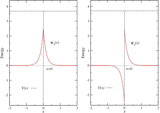
Figure 1: Left panel: Ground state wave function for a parity-invariant point interaction with $a=d=1$, $b=0$, $\theta=0$. The horizontal dashed lines indicate the potential $V(x)$. The downward vertical dashed line symbolizes an attractive point interaction at $x_{0}=0$, equivalent to a $\delta$-function potential. Right panel: Ground state wave function for a parity-invariant point interaction with $a=d=-1$, $b=0$, $\theta=0$.

Let us also consider scattering states, first for $H$, and no longer assuming parity symmetry. We make the ansatz

$$\Psi_{k}(x)=\exp(ikx)+R\exp(-ikx),\ x<0,\quad\Psi_{k}(x)=T\exp(ikx),\ x>0,$$ (3.20)

which implies

$$\left(\begin{array}[]{c}T\\ ikT\end{array}\right)=\exp(i\theta)\left(\begin{array}[]{cc}a&0\\ c&1/a\end{array}\right)\left(\begin{array}[]{c}1+R\\ ik(1-R)\end{array}\right)\ \Rightarrow$$ (3.27)

$$R=\frac{ik(1-a^{2})+ac}{ik(1+a^{2})-ac},\quad T=\frac{2ika\exp(i\theta)}{ik(1+a^{2})-ac}.$$ (3.28)

Similarly, for the superpartner one obtains

$$R^{\prime}=\frac{ik(1-{a^{\prime}}^{2})+a^{\prime}c^{\prime}}{ik(1+{a^{\prime}}^{2})-a^{\prime}c^{\prime}}=\frac{ik(a^{2}-1)-ac}{ik(a^{2}+1)+ac},$$

$$T^{\prime}=\frac{2ika^{\prime}\exp(i\theta)}{ik(1+{a^{\prime}}^{2})-a^{\prime}c^{\prime}}=\frac{2ika\exp(i\theta)}{ik(a^{2}+1)+ac}.$$ (3.29)

In particular, one obtains $|R^{\prime}|=|R|$, $|T^{\prime}|=|T|$.

3.3 Self-Adjoint Extensions of a Particle in a Box

Let us now consider a particle in a box of size $L$ ($x\in[-L/2,L/2]$) with a general Robin boundary condition characterized by the self-adjoint extension parameter $\gamma$. In order to ensure parity symmetry, we impose the boundary condition in a symmetric manner such that

$$\partial_{x}\Psi(L/2)+\gamma\Psi(L/2)=0,\quad\partial_{x}\Psi(-L/2)-\gamma\Psi(-L/2)=0.$$ (3.30)

The Dirichlet boundary condition that is used in standard textbook treatments corresponds to $\gamma=\infty$. A detailed discussion for general values of $\gamma$ can be found in [8]. The resulting spectra and wave functions are illustrated in figure 2.

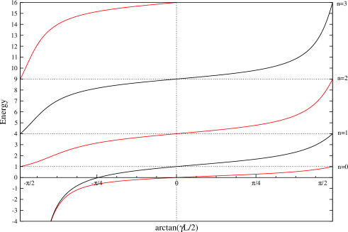
Figure 2: Top panel: Energy spectrum of a particle in a box as a function of the self-adjoint extension parameter $\gamma$. The $x$-value represents $\arctan(\gamma L/2)\in[-\tfrac{\pi}{2},\tfrac{\pi}{2}]$, which corresponds to $\gamma\in[-\infty,\infty]$. The $y$-value represents the energies $E_{n}$ (with $n=0,1,2,3,4$) in units of $\pi^{2}/(2mL^{2})$. Bottom panel: The wave functions $\Psi_{n}(x)$, $x\in[-\tfrac{L}{2},\tfrac{L}{2}]$, (with $n=0,1,2,3$), for $\gamma=-\infty,-\tfrac{2}{L},0,\infty$. The sharp peaks in the $n=0$ and $n=1$ states at $\gamma=-\infty$ represent $\delta$-function-type wave functions of negative infinite energy localized at the boundaries. Except for these states, the energies and wave functions at $\gamma=-\infty$ are the same as those at $\gamma=\infty$.

The case $\gamma=0$ corresponds to Neumann boundary conditions, for which the ground state has zero energy. For $\gamma<0$, there are even negative energy states, localized at the wall. This seems to contradict the Heisenberg uncertainty relation, which, however, applies only to the infinite volume. A generalized uncertainty relation, which applies to a finite volume, was derived in [8], and is consistent with negative energy values.

For $\gamma>0$, the even parity states take the form

$$\Psi_{n}(x)=B\cos(k_{n}x),\ \frac{\gamma}{k_{n}}=\tan(k_{n}L/2),\ n=0,2,4,\dots,$$ (3.31)

while the odd parity states are given by

$$\Psi_{n}(x)=C\sin(k_{n}x),\ \frac{\gamma}{k_{n}}=-\cot(k_{n}L/2),\ n=1,3,5,\dots.$$ (3.32)

The superpotential thus takes the form

$$W(x)=-\frac{\partial_{x}\Psi_{0}(x)}{\Psi_{0}(x)}=k_{0}\tan(k_{0}x),$$ (3.33)

such that

$$2mV(x)=-\partial_{x}W(x)+W(x)^{2}=-k_{0}^{2},$$

$$2mV^{\prime}(x)=\partial_{x}W(x)+W(x)^{2}=k_{0}^{2}\left(\frac{2}{\cos^{2}(k_{0}x)}-1\right).$$ (3.34)

The ground state of the first supersymmetric descendant is obtained as

$$\Psi_{1}^{\prime}(x)=\frac{1}{\sqrt{\lambda_{1}}}[\partial_{x}+W(x)]\Psi_{1}(x)=\frac{C}{\sqrt{k_{1}^{2}-k_{0}^{2}}}[k_{1}\cos(k_{1}x)+k_{0}\tan(k_{0}x)\sin(k_{1}x)],$$ (3.35)

which gives rise to the next superpotential

$$W^{\prime}(x)=-\frac{\partial_{x}\Psi_{1}^{\prime}(x)}{\Psi_{1}^{\prime}(x)}=\frac{(k_{1}^{2}-k_{0}^{2})\sin(k_{1}x)}{k_{1}\cos(k_{1}x)+k_{0}\tan(k_{0}x)\sin(k_{1}x)}-k_{0}\tan(k_{0}x).$$ (3.36)

Based on this, it is straightforward to work out the potential $V^{\prime\prime}(x)$ of the second descendant. However, the expression is not very illuminating, and we thus do not show it here.

It is instructive to consider special cases of the self-adjoint extension parameter $\gamma$, starting with the standard textbook case $\gamma=\infty$. The various potentials and the corresponding wave functions of the lowest energy eigenstates are illustrated for the original Hamiltonian $H$ and its supersymmetric descendants $H^{\prime}$ and $H^{\prime\prime}$ in figure 3.

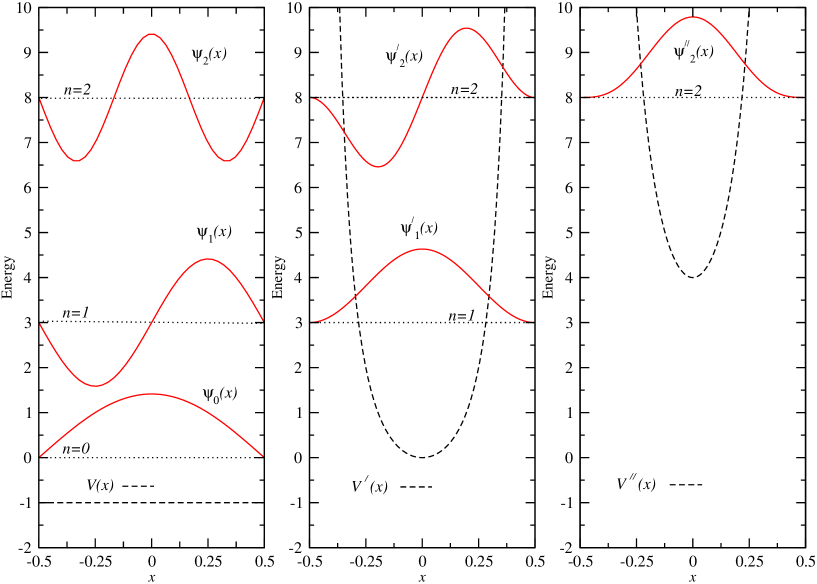
Figure 3: A particle in a box with standard Dirichlet boundary conditions (i.e. $\gamma=\infty$). The original system (left panel) is compared to its first two supersymmetric descendants (middle and right panel). The corresponding potentials $V(x)$, $V^{\prime}(x)$, and $V^{\prime\prime}(x)$ are shown together with the low-energy spectrum (horizontal dotted lines). The wave functions $\Psi_{n}(x)$, $\Psi_{n}^{\prime}(x)$, and $\Psi_{n}^{\prime\prime}(x)$ are drawn using the corresponding energy level as the $x$-axis.

The $\gamma=0$ case, which corresponds to Neumann boundary conditions, is illustrated in figure 4. In that case, the ground state has a constant wave function $\Psi_{0}(x)=\sqrt{1/L}$ of zero energy. Hence, the superpotential simply vanishes, i.e. $W(x)=0$, and, in addition, $V(x)=V^{\prime}(x)=0$. Since the superpartner always obeys Dirichlet boundary conditions, i.e. $\gamma^{\prime}=\infty$, in this case the first supersymmetric descendant coincides with the standard textbook case of a particle in a box.

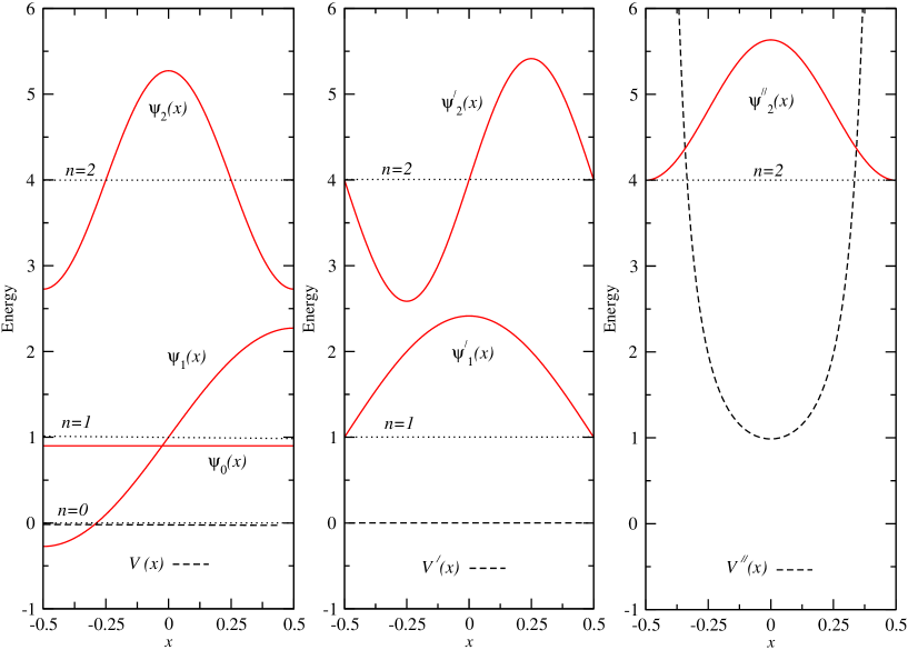
Figure 4: A particle in a box with Neumann boundary conditions (i.e. $\gamma=0$). The original system (left panel) is compared to its first two supersymmetric descendants (middle and right panel). The corresponding potentials $V(x)$, $V^{\prime}(x)$, and $V^{\prime\prime}(x)$ are shown together with the low-energy spectrum (horizontal dotted lines). The wave functions $\Psi_{n}(x)$, $\Psi_{n}^{\prime}(x)$, and $\Psi_{n}^{\prime\prime}(x)$ are drawn using the corresponding energy level as the $x$-axis.

For $\gamma<0$, the ground state has negative energy, and is given by

$$\Psi_{0}(x)=B\cosh(\varkappa_{+}x),\ \frac{\gamma}{\varkappa_{+}}=-\tanh(\varkappa_{+}L/2),$$ (3.37)

such that the superpotential then takes the form

$$W(x)=-\frac{\partial_{x}\Psi_{0}(x)}{\Psi_{0}(x)}=-\varkappa_{+}\tanh(\varkappa_{+}x).$$ (3.38)

We thus obtain

$$2mV(x)=-\partial_{x}W(x)+W(x)^{2}=\varkappa_{+}^{2},$$

$$2mV^{\prime}(x)=\partial_{x}W(x)+W(x)^{2}=\varkappa_{+}^{2}\left(1-\frac{2}{\cosh^{2}(\varkappa_{+}x)}\right).$$ (3.39)

For $-2/L<\gamma<0$, the first excited state has positive energy and is still given by eq.(3.32). The ground state of the first supersymmetric descendant is then obtained as

$$\Psi_{1}^{\prime}(x)=\frac{1}{\sqrt{\lambda_{1}}}[\partial_{x}+W(x)]\Psi_{1}(x)=\frac{C}{\sqrt{k_{1}^{2}+\varkappa_{+}^{2}}}[k_{1}\cos(k_{1}x)-\varkappa_{+}\tanh(\varkappa_{+}x)\sin(k_{1}x)],$$ (3.40)

which gives rise to the next superpotential

$$W^{\prime}(x)=-\frac{\partial_{x}\Psi_{1}^{\prime}(x)}{\Psi_{1}^{\prime}(x)}=\frac{(k_{1}^{2}+\varkappa_{+}^{2})\sin(k_{1}x)}{k_{1}\cos(k_{1}x)-\varkappa_{+}\tanh(\varkappa_{+}x)\sin(k_{1}x)}+\varkappa_{+}\tanh(\varkappa_{+}x).$$ (3.41)

The special case $\gamma=-2/L$ is illustrated in figure 5. In that case, the first excited state, $\Psi_{1}(x)=\sqrt{12/L^{3}}x$, has zero energy.

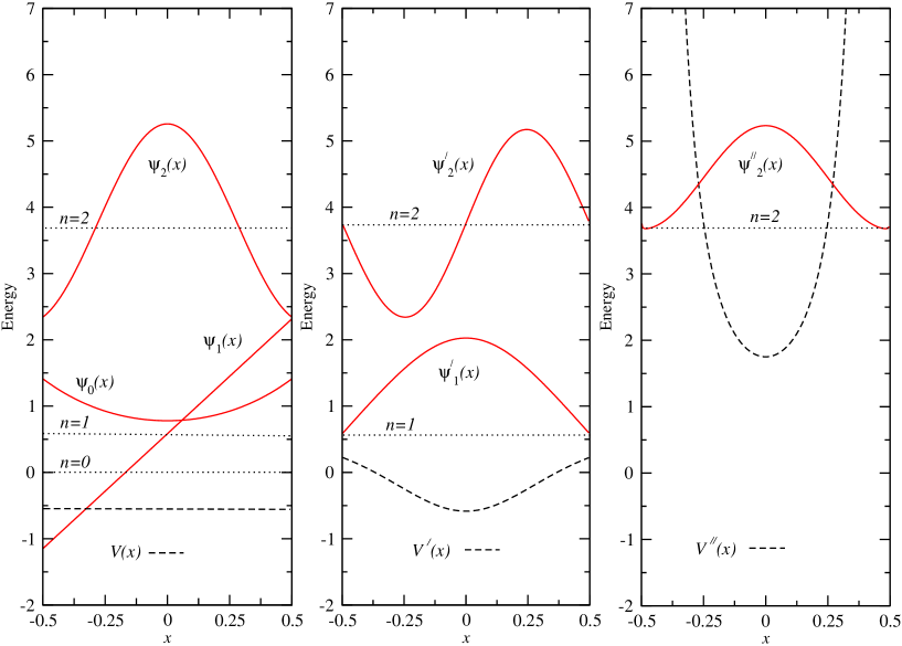
Figure 5: A particle in a box with $\gamma=-2/L$. The original system (left panel) is compared to its first two supersymmetric descendants (middle and right panel). The corresponding potentials $V(x)$, $V^{\prime}(x)$, and $V^{\prime\prime}(x)$ are shown together with the low-energy spectrum (horizontal dotted lines). The wave functions $\Psi_{n}(x)$, $\Psi_{n}^{\prime}(x)$, and $\Psi_{n}^{\prime\prime}(x)$ are drawn using the corresponding energy level as the $x$-axis.

For completeness, let us finally investigate the case $\gamma<-2/L$. Then both the ground state of eq.(3.37) and the first excited state have negative energy, and

$$\Psi_{1}(x)=C\sinh(\varkappa_{-}x),\ \frac{\gamma}{\varkappa_{-}}=-\coth(\varkappa_{-}L/2).$$ (3.42)

The ground state of the first supersymmetric descendant is now given by

$$\Psi_{1}^{\prime}(x) = \frac{1}{\sqrt{\lambda_{1}}}[\partial_{x}+W(x)]\Psi_{1}(x)$$ (3.43)

$$= \frac{C}{\sqrt{\varkappa_{+}^{2}-\varkappa_{-}^{2}}}[\varkappa_{-}\cosh(\varkappa_{-}x)-\varkappa_{+}\tanh(\varkappa_{+}x)\sinh(\varkappa_{-}x)],$$

which gives rise to the next superpotential

$$W^{\prime}(x)=-\frac{\partial_{x}\Psi_{1}^{\prime}(x)}{\Psi_{1}^{\prime}(x)}=\frac{(\varkappa_{+}^{2}-\varkappa_{-}^{2})\sinh(\varkappa_{-}x)}{\varkappa_{-}\cosh(\varkappa_{-}x)-\varkappa_{+}\tanh(\varkappa_{+}x)\sinh(\varkappa_{-}x)}+\varkappa_{+}\tanh(\varkappa_{+}x).$$ (3.44)

3.4 Particle in a Box with an Additional Point Interaction

In this subsection, we consider a particle in a box with Robin boundary conditions characterized by the self-adjoint extension parameter $\gamma$, subject to an additional parity-invariant point interaction at $x_{0}=0$, described by the self-adjoint extension parameters $a=\pm 1$ and $c$.

First, we consider positive energy states of even parity for which

$$\Psi_{k+}(x)=D_{+}\cos(k|x|+\delta).$$ (3.45)

It is straightforward to work out the equation for the corresponding energy values. For $a=1$, one obtains

$$\tan\delta=-\frac{c}{2k},\quad\frac{2\gamma+c}{2k-c\gamma/k}=\tan(kL/2),$$ (3.46)

while for $a=-1$

$$\cos\delta=0,\quad\frac{\gamma}{k}=-\cot(kL/2),$$ (3.47)

Similarly, for the parity-odd states of positive energy one has

$$\Psi_{k-}(x)=D_{-}\text{sign}(x)\cos(k|x|+\delta).$$ (3.48)

In that case, for $a=1$, one obtains

$$\cos\delta=0,\quad\frac{\gamma}{k}=-\cot(kL/2),$$ (3.49)

while for $a=-1$

$$\tan\delta=\frac{c}{2k},\quad\frac{2\gamma-c}{2k+c\gamma/k}=\tan(kL/2),$$ (3.50)

This shows that the energy spectrum of the even (odd) parity states for $a=1$ and $c$ is the same as the one of the odd (even) parity states for $a=-1$ and $-c$.

Let us also consider negative energy states, first with even parity

$$\Psi_{+}(x)=B_{+}\exp(-\varkappa_{+}|x|)+C_{+}\exp(\varkappa_{+}|x|).$$ (3.51)

For $a=1$, one then obtains

$$\frac{(\varkappa_{+}-\gamma)(2\varkappa_{+}-c)}{(\varkappa_{+}+\gamma)(2\varkappa_{+}+c)}=\exp(\varkappa_{+}L),$$ (3.52)

while for $a=-1$

$$\frac{\gamma}{\varkappa_{+}}=-\tanh(\varkappa_{+}L/2).$$ (3.53)

Similarly, for the negative energy states with odd parity

$$\Psi_{-}(x)=\text{sign}(x)[B_{-}\exp(-\varkappa_{+}|x|)+C_{-}\exp(\varkappa_{+}|x|)],$$ (3.54)

with $a=1$ one finds

$$\frac{\gamma}{\varkappa_{-}}=-\coth(\varkappa_{-}L/2),$$ (3.55)

and with $a=-1$ one obtains

$$\frac{(\varkappa_{-}-\gamma)(2\varkappa_{-}+c)}{(\varkappa_{-}+\gamma)(2\varkappa_{-}-c)}=\exp(\varkappa_{-}L).$$ (3.56)

The corresponding energy spectrum is illustrated in figure 6, both for a repulsive and for an attractive point interaction.

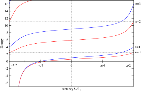
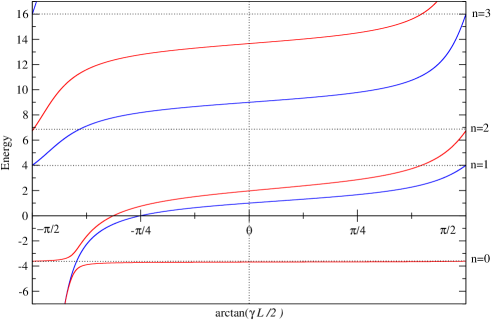
Figure 6: Energy spectrum of a particle in a box as a function of the self-adjoint extension parameter $\gamma$ with a repulsive (top panel) or attractive (bottom panel) point interaction with $c=\pm 12m$. The $x$-value represents $\arctan(\gamma L/2)\in[-\tfrac{\pi}{2},\tfrac{\pi}{2}]$, which corresponds to $\gamma\in[-\infty,\infty]$. The $y$-value represents the energies $E_{n}$ (with $n=0,1,2,3$) in units of $\pi^{2}/(2mL^{2})$. The states with odd $n$ are unaffected by the point interaction and are identical with those of a particle in a box without point interaction (figure 2).

3.5 Bulk-Boundary Resonance and its Supersymmetric Descendant

In the bottom panel of figure 6, at negative values of $\gamma$, one notices an avoided level crossing between the ground state and the second excited state. Such avoided level crossings are characteristic of a resonance in a finite volume [40, 41]. In this case, we encounter a bulk-boundary resonance, with the particle partially localized at the walls, and partially at the center of the box, due to the attractive point interaction. For definiteness, we set $a=1$. The situation for $a=-1$ is analogous.

As a resonance condition, let us demand equal probability density at the walls and at the center, i.e. $|\Psi_{+}(\pm L/2)|^{2}=|\Psi_{+}(0)|^{2}$. It is easy to convince oneself that this implies $c=2\gamma$, in which case the ground state wave function reduces to

$$\Psi_{0}(x)=\Psi_{+}(x)=B\cosh[\varkappa_{+}(|x|-L/4)],\ \frac{\gamma}{\varkappa_{+}}=-\tanh(\varkappa_{+}L/4),\ \varkappa_{+}>-\gamma.$$ (3.57)

The first excited state takes the form

$$\Psi_{1}(x)=\Psi_{-}(x)=C\sinh(\varkappa_{-}x),\quad\frac{\gamma}{\varkappa_{-}}=-\coth(\varkappa_{-}L/2),$$ (3.58)

while the second excited state, which resonates with $\Psi_{0}(x)$, is given by

$$\Psi_{2}(x)=\widetilde{\Psi}_{+}(x)=-D\sinh[\widetilde{\varkappa}_{+}(|x|-L/4)],$$

$$\frac{\gamma}{\widetilde{\varkappa}_{+}}=-\coth(\widetilde{\varkappa}_{+}L/4),\ \widetilde{\varkappa}_{+}<-\gamma.$$ (3.59)

These wave functions and their energies are illustrated in the left panel of figure 7.

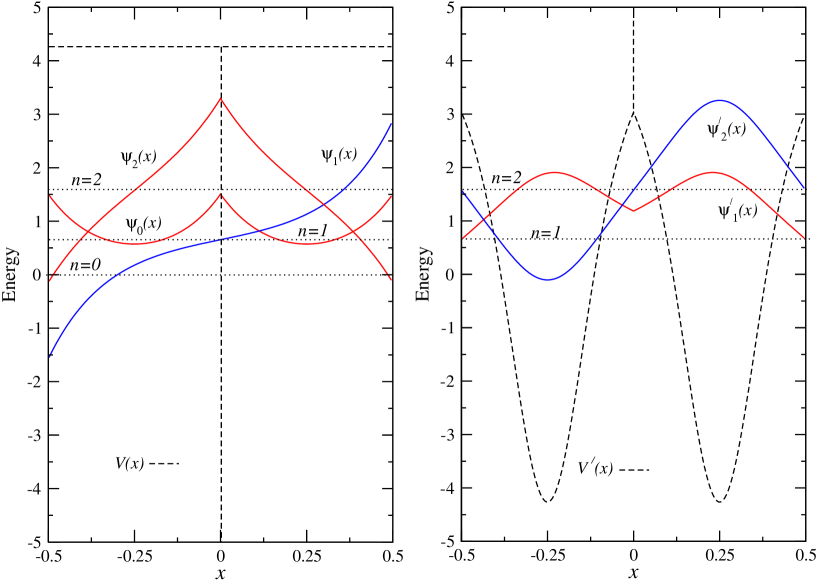
Figure 7: A bulk-boundary resonance of a particle in a box with an additional point interaction with $a=1$. The original system (left panel) is compared to its supersymmetric descendant (right panel). The corresponding potentials $V(x)$ and $V^{\prime}(x)$ are shown together with the low-energy spectrum (horizontal dotted lines). The wave functions $\Psi_{n}(x)$ and $\Psi_{n}^{\prime}(x)$ are drawn using the corresponding energy level as the $x$-axis. The downward and upward vertical dashed lines symbolize an attractive or repulsive point interaction, respectively.

Let us now construct the superpotential associated with the bulk-boundary resonance

$$W(x)=-\frac{\partial_{x}\Psi_{0}(x)}{\Psi_{0}(x)}=-\varkappa_{+}\text{sign}(x)\tanh[\varkappa_{+}(|x|-L/4)].$$ (3.60)

The original potential and that of the superpartner then take the form

$$2mV(x)=-\partial_{x}W(x)+W(x)^{2}=\varkappa_{+}^{2}$$

$$2mV^{\prime}(x)=\partial_{x}W(x)+W(x)^{2}=\varkappa_{+}^{2}\left(1-\frac{2}{\cosh^{2}[\varkappa_{+}(|x|-L/4)]}\right).$$ (3.61)

Interestingly, $V^{\prime}(x)$ represents a double-well potential, with a repulsive point interaction at $x_{0}=0$, characterized by

$$c^{\prime}=-c=-2\gamma=2\varkappa_{+}\tanh(\varkappa_{+}L/4).$$ (3.62)

The ground and first excited state of the supersymmetric descendant are given by

$$\Psi_{1}^{\prime}(x)\!\! = \!\!\frac{1}{\sqrt{\lambda_{1}}}[\partial_{x}+W(x)]\Psi_{1}(x)$$

$$= \!\!\frac{C}{\sqrt{\varkappa_{+}^{2}-\varkappa_{-}^{2}}}\{\varkappa_{-}\cosh(\varkappa_{-}x)-\text{sign}(x)\varkappa_{+}\tanh[\varkappa_{+}(|x|-L/4)]\sinh(\varkappa_{-}x)\},$$

$$\Psi_{2}^{\prime}(x)\!\! = \!\!\frac{1}{\sqrt{\lambda_{2}}}[\partial_{x}+W(x)]\Psi_{2}(x)$$ (3.63)

$$= \!\!\frac{D\text{sign}(x)}{\sqrt{\varkappa_{+}^{2}-\widetilde{\varkappa}_{+}^{2}}}\{\widetilde{\varkappa}_{+}\cosh[\widetilde{\varkappa}_{+}(|x|-L/4)]$$

$$- \!\!\varkappa_{+}\tanh[\varkappa_{+}(|x|-L/4)]\sinh[\widetilde{\varkappa}_{+}(|x|-L/4)]\}.$$

These states together with the corresponding potential $V^{\prime}(x)$ are illustrated in the right panel of figure 7.

In the original system, the first excited state is unaffected by the point interaction and is identical with the one of just the particle in the box. The ground state and the second excited state, on the other hand, resonate with one another and are both localized on the walls as well as on the puncture at $x_{0}=0$. In the spectrum, the resonance manifests itself by an avoided level crossing. When one proceeds to the supersymmetric descendant, the ground state is removed and the first excited state of the original system turns into the ground state of the superpartner. Interestingly, while this state was unaffected by the attractive point interaction of the original system, it is affected by the repulsive point interaction of the supersymmetric descendant. Similarly, the second excited state of the original system, which was affected by the attractive point interaction, turns into the first excited state of the superpartner, but is now unaffected by its repulsive point interaction. What has become of the resonance of the two states, now that the original ground state has been removed from the supersymmetric descendant? As we see from the right panel of figure 7, the superpartner has a double-well potential, and its ground and first excited states are almost degenerate, with a splitting due to tunneling processes between the two wells. Indeed, the regions near the walls and near the puncture, which were energetically favored in the original system, are disfavored in the supersymmetric descendant. This shows how one and the same spectrum (except for the ground state $\Psi_{0}(x)$) can arise from quite different physical phenomena, in one case a bulk-boundary resonance, in the other case tunneling in a double-well potential.

The corresponding situation for $a=-1$ is illustrated in figure 8, which confirms that the spectrum is the same as for $a=1$, but even and odd parity states exchange their roles. In particular, the ground state is now parity-odd, and the first excited state is parity-even.

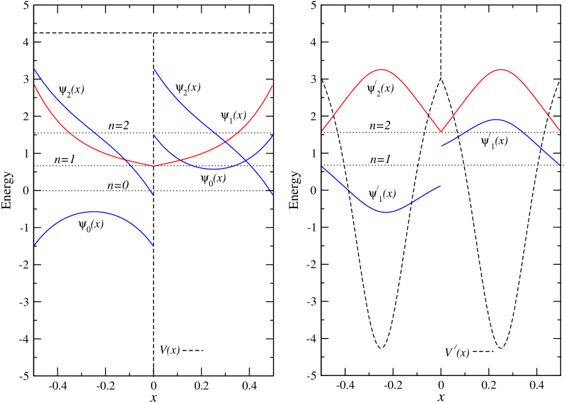
Figure 8: A bulk-boundary resonance of a particle in a box with an additional point interaction with $a=-1$. The original system (left panel) is compared to its supersymmetric descendant (right panel). The corresponding potentials $V(x)$ and $V^{\prime}(x)$ are shown together with the low-energy spectrum (horizontal dotted lines). The wave functions $\Psi_{n}(x)$ and $\Psi_{n}^{\prime}(x)$ are drawn using the corresponding energy level as the $x$-axis. The downward and upward vertical dashed lines symbolize an attractive or repulsive point interaction, respectively.

4 Conclusions

We have investigated the supersymmetric descendants of self-adjointly extended Hamiltonians. The infinite-wall boundary condition of a particle on a half-line is characterized by a family of self-adjoint extensions, parameterized by $\gamma\in{\mathbb{R}}$. Interestingly, all corresponding supersymmetric descendants have $\gamma^{\prime}=\infty$ and thus obey standard Dirichlet boundary conditions. A particle on a punctured line with a point interaction at the puncture $x_{0}$ is characterized by a 4-parameter family of self-adjoint extensions. Remarkably, in that case, the corresponding supersymmetric descendants are not automatically self-adjoint. Indeed, only a 3-parameter sub-family of Hamiltonians has supersymmetric descendants which are themselves self-adjoint. This sub-family is characterized by the continuity of the probability density at the puncture.

We have also constructed the self-adjoint extensions of the operator ${\cal Q}_{+}$ constructed from the supercharge. They form a 1-parameter family on the half-line, and a 4-parameter family on the punctured line. Yet, only one specific value of the self-adjoint extension parameter (namely $\eta=0$) is physical on the half-line, and only a 2-parameter sub-class is physical on the punctured line. This is because we have considered $H$ and $H^{\prime}$ as two distinct physical systems, and not as two parts of a bigger system. While there is a 1-parameter family of self-adjoint extensions of $H$ on the half-line (parameterized by $\gamma$), there is no remaining self-adjoint extension parameter in ${\cal Q}_{+}$, after we put $\eta=0$. This is because the information on $\gamma$ is encoded in the superpotential. Similarly, on the punctured line there is a 3-parameter family of self-adjoint extensions of $H$ (parameterized by $a$, $c$, and $\theta$), for which the supersymmetric descendant $H^{\prime}$ is also self-adjoint. At the same time, there is only a 2-parameter family of self-adjoint extensions of ${\cal Q}_{+}$ (parameterized by $a$ and $\theta$). This is again because the information about the third parameter $c$ is encoded in the superpotential. This clarifies the relations between the self-adjoint extensions of $H$, $H^{\prime}$, and ${\cal Q}_{+}$.

We have also examined concrete problems of a particle in a box, with or without an additional point interaction. Among other things, we found that the standard textbook problem of a particle in a box with Dirichlet boundary conditions is itself a supersymmetric descendant. Its supersymmetric precursor is the corresponding problem with Neumann boundary conditions. Robin boundary conditions with $\gamma<0$ give rise to negative energy states localized at the walls. Such boundary states can resonate with states localized in the bulk, which gives rise to an avoided level crossing in a finite volume. We have investigated the supersymmetric descendant of such a resonance and found that it corresponds to two almost degenerate states in a double-well potential.

By applying self-adjoint extensions to supersymmetric quantum mechanics, we have extended the set of exactly solvable quantum mechanics problems. Self-adjoint extensions are not just a mathematical curiosity, but have great physical relevance. The self-adjoint extension parameters just characterize the low-energy features of an idealized boundary, such as an impenetrable infinite energy barrier, or an ultra-short-range attractive potential in a tiny region of space. Using the theory of self-adjoint extensions greatly simplifies the modeling of such situations. In fact, some of the calculations performed here are so simple that they could easily be incorporated into the teaching of quantum mechanics. We conclude this paper by expressing our hope that, in the future, the powerful theory of self-adjoint extensions may make a stronger appearance in textbooks and in the teaching of quantum mechanics.

References

- [1] M. Reed and B. Simon, Methods of Modern Mathematical Physics II, Fourier Analysis, Self-Adjointness, Academic Press Inc., New York (1975).
- [2] J. von Neumann, Mathematische Grundlagen der Quantenmechanik, Berlin, Springer (1932).
- [3] G. Bonneau, J. Faraut, and G. Valent, Am. J. Phys. 69 (2001) 322.
- [4] F. A. Berezin and L. D. Faddeev, Dokl. Akad. Nauk SSSR 137 (1961) 1011.
- [5] S. Albeverio, F. Gesztesy, R. Hoeg-Krohn, and H. Holden, Solvable Models in Quantum Mechanics, Texts and Monographs, Springer, New York (1988).
- [6] R. Jackiw, M. A. B. Beg Memorial Volume, A. Ali and P. Hoodbhoy, Eds., World Scientific, Singapore (1991).
- [7] M. Carreau and E. Farhi, Phys. Rev. D42 (1990) 1194.
- [8] M. H. Al-Hashimi and U.-J. Wiese, Ann. Phys. 327 (2012) 1.
- [9] P. Harrison, Quantum wells, wires and dots, John Wiley and Sons Ltd. (2005).
- [10] P. de Sousa Gerbert and R. Jackiw, Commun. Math. Phys. 124 (1989) 229.
- [11] P. de Sousa Gerbert, Phys. Rev. D40 (1989) 1346.
- [12] Y. A. Sitenko, Phys. Lett. B387 (1996) 334.
- [13] M. H. Al-Hashimi and U.-J. Wiese, Ann. Phys. 323 (2008) 92.
- [14] E. N. Dancer and D. Daners, J. Diff. Equ. 138 (1997) 86.
- [15] W. Arendt and M. Warma, J. Evol. Equ. 3 (2003) 119.
- [16] W. Arendt and M. Warma, Potential Anal. 19 (2003) 341.
- [17] K. Pankrashkin, Rep. Math. Phys. 58 (2006) 207.
- [18] R. Balian and C. Bloch, Ann. Phys. 60 (1970) 401.
- [19] A. V. Scherbinin and V. I. Pupyshev, Russ. J. Phys. Chem. 74 (2000) 292.
- [20] S. L. Lebedev, JETP 83 (1996) 423.
- [21] L. C. de Albuquerque and R. M. Cavalcanti, J. Phys. A37 (2004) 7039.
- [22] P. Minces and V. O. Rivelles, Nucl. Phys. B572 (2000) 651.
- [23] Advances in Quantum Chemistry 57, Theory of confined quantum systems, edited by J. R. Sabin, E. Brändas, and S. A. Cruz, Academic Press, Elsevier (2009).
- [24] M. H. Al-Hashimi, Mol. Phys. 111 (2013) 225.
- [25] M. H. Al-Hashimi and U.-J. Wiese, Ann. Phys. 327 (2012) 2742.
- [26] V. I. Pupyshev and A. V. Scherbinin, Chem. Phys. Lett. 295 (1998) 217.
- [27] V. I. Pupyshev and A. V. Scherbinin, Phys. Lett. A 299 (2002) 371.
- [28] E. Witten, Nucl. Phys. B188 (1981) 513.
- [29] F. Cooper and B. Freedman, Ann. Phys. 146 (1983) 262.
- [30] F. Cooper, A. Khare, and U. Sukhatme, “Supersymmetry in Quantum Mechanics”, World Scientific, Singapore (2001).
- [31] B. K. Bagchi, “Supersymmetry in Quantum and Classical Mechanics”, Monographs and Surveys in Pure and Applied Mathematics 116, Chapman and Hall, CRC Press (2001).
- [32] T. Cheon, T. Fülöp, and I. Tsutsui, Ann. Phys. 294 (2001) 1.
- [33] T. Uchino and I. Tsutsui, Nucl. Phys. B662 (2003) 447.
- [34] T. Uchino and I. Tsutsui, J. Phys. A36 (2003) 6821.
- [35] T. Nagasawa, M. Sakamoto, and K. Takenaga, Phys. Lett. B562 (2003) 358.
- [36] T. Nagasawa, M. Sakamoto, and K. Takenaga, Phys. Lett. B583 (2004) 357.
- [37] H. Falomir and P. A. G. Pisani, J. Phys. A38 (2005) 4665.
- [38] M. J. Puska and R. M. Niemenin, Phys. Rev. A 47 (1993) 1181.
- [39] G. Wendin and B. Wästberg, Phys. Rev. B 48 (1993) 14764.
- [40] U.-J. Wiese, Nucl. Phys. Proc. Suppl. 9 (1989) 609.
- [41] M. Lüscher, Nucl. Phys. B364 (1991) 237.