Spin Dynamics of Trimers on a Distorted Kagomé Lattice

Abstract

We treat the ground state, elementary excitations, and neutron scattering cross section for a system of trimers consisting of three tightly bound spins 1/2 on a distorted Kagomé lattice, subject to isotropic nearest neighbor (usually antiferromagnetic) Heisenberg interactions. The interactions between trimers are assumed to be weak compared to the intra trimer interactions. We compare the spin-wave excitation spectrum of trimers with that obtained from standard spin-wave theory and attribute the differences at low energy to the fact that the trimer formulation includes exactly the effects of intra-trimer zero point motion. Application to existing systems is briefly discussed.

I INTRODUCTION

Frustrated antiferromagnetic systems have received enormous attention in recent years.MW ; GN ; KSB One limit which has attracted less attention is that when the frustration is removed by the formation of strongly coupled three-spin units called spin trimers.JAPS ; CB ; FURRER1 ; FURRER2 ; POD ; OKAM ; HL Early experiments and calculations were performed for high ($S=5/2)$ spin states of Fe³⁺ and Mn²⁺ by Falk et al.,FURRER1 and Furrer and Güdel.FURRER2 For $S=1/2$ systems much work has been focused on chain-like systems consisting of trimers of Cu ions.JAPS ; OKAM ; HL Other configurations of trimers were studied by Qiu et al.,CB and Podlesnyak et al.POD In these works the interactions between trimers were very weak, so that the energy of the localized excitations appeared not to depend on wave vector. In that case, information on the nature of the excited states of the trimers was obtained by monitoring the dependence of the magnitude of the inelastic scattering cross section on wave vector. In contrast, here we will consider a system of interacting spin 1/2 trimers where the excitations have a significant dependence on wave vector. We implement perturbation theory by introducing operators which create or destroy the the exact excited states of isolated trimers. In the limit when the inter-trimer interactions vanish, our calculation reduces to those of Refs. FURRER1, and CB, .

The system of trimers of spins 1/2 we consider is specified by Fig. 1 where we show the covering of a distorted Kagomé lattice by trimers. The lattice has the connectivity of a Kagomé lattice, but lacks its three-fold symmetry, so that the nearest neighbor isotropic exchange interactions assume three values $J$, $j$, and $k$, of which $J$ is assumed to be dominant. This model may be an appropriate one for the distorted Kagomé system Cu₂(OD)₃Cl.SHL1 ; SHL2 Even if this system is not an ideal representative of the model we introduce below, our results may stimulate the search for better realizations of our model. The aim of this paper is to develop a calculation which is correct to leading order in $j/J$ and $k/J$ and to compare results obtained in this approximation to standard spin-wave theory, based on the Néel state which treats all the exchange interactions on an equal footing. We find that there is a one-to-one mapping connecting the lowest energy manifold of excitations in the two approaches and that the differences in energies can be understood in terms of the differing way quantum zero-point motion is treated in the two approaches. At higher energy the comparison is more complicated. In the trimer approach one does have the higher energy transverse spin waves of the Néel state. But in addition, some of the higher energy trimer excitations correspond to bound states of two or more Néel-state spin excitations. The trimer approach is clearly superior when the intertrimer interactions are perturbative, as we assume in this paper.

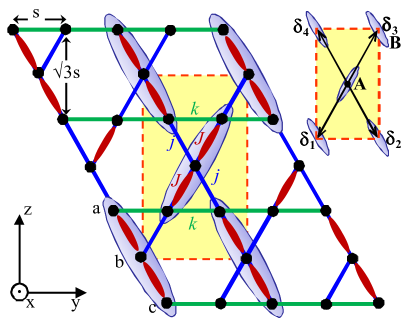
Figure 1: (Color online) A distorted Kagomé lattice with three isotropic nearest neighbor Heisenberg interactions; $J$ (red), $j$ (blue) and $k$ (green). We assume $J$ is antiferromagnetic and much larger than $j$ and $k$, yielding spin trimers (some of which are shown as ellipses) which consist of three spins connected by two large interactions, $J$. The dashed rectangle is the unit cell containing two trimers, A and B. The upper right inset shows the four nearest neighbor vectors of the trimer lattice as given in Eq. (14). Here $s$ is the nearest neighbor separation between spins on the Kagomé lattice. The labeling of the three sites within a trimer is $a$, $b$, $c$ in the order of decreasing $z$ coordinate, as shown for a trimer in the left bottom corner of the unit cell.

Briefly, this paper is organized as follows. In Sec. II we give a qualitative overview of the calculation in which the intertrimer interactions $j$ and $k$ are treated perturbatively with respect to the strong intratrimer interaction $J$. In Sec. III we show that the low energy manifold of spin waves can be mapped onto the usual manifold of spin waves, but with an effective trimer-trimer interaction playing the role of the usual spin-spin interaction. Here and in succeeding sections we treat the two cases when a) the net spins of adjacent trimers are coupled antiferromagnetically and b) the net spins of adjacent trimers are coupled ferromagnetically. In Sec. IV we consider the exciton spectrum in which trimers are promoted into their nearly localized excited states. In Sec. V we present results of standard spin-wave calculations based on the Néel state in which all spins in the ground state have $S_{z}=1/2$ or $S_{z}=-1/2$. In Sec VI we compare the results the spin-wave and perturbative approaches give for the elastic diffraction pattern. We attribute the differences in results to the differences in how quantum zero-point motion is treated in the two approaches. In Sec. VII we consider the inelastic neutron scattering cross section from the entire spectrum of trimer excitations. Our results are summarized and briefly discussed in Sec. VIII.

II OVERVIEW

In the magnetically disordered phase of Cu(OD)₃Cl (which we take as the exemplar of our trimer model) the unit cell shown in Fig. 1 contains six Cu spin sites. In Fig. 2 we show the phase diagram of the trimer model as a function of the temperature $T$ when $J$ is much larger than either $j$ or $k$. When $T$ is large compared to $J$ the spins are essentially uncorrelated. As $T$ is reduced to become comparable to $J$, one passes through a regime in which the correlations within spin trimers become well developed. In Fig. 2, this regime is labeled ”trimer melting.” Below this regime the average spin of the middle site of the trimer is oppositely oriented to those of the end sites of the trimer.[SHL1, ; SHL2, ] However, as long as $T>T_{c}$, the spin correlation function between different trimers decays rapidly as a function of their separation. When $T$ is reduced so as to be comparable to $j$ and/or $k$, one passes through a phase transition (at $T=T_{c}$) below which one has long range spin order. As we discuss below, depending on how $j$ and $k$ compare, the adjacent trimers can either be organized ferromagnetically or antiferromagnetically. In either case, the magnetic ordering occurs at zero wave vector. In other words, the magnetic and paramagnetic unit cells are identical, each containing two trimer units. As we shall see, when $T\ll T_{c}$ the elementary excitations are identical to spin waves in the usual magnetic systems.

In contrast and as will become apparent, the higher energy trimer excitons are qualitatively different from the higher energy spin wave relative to the Néel ground state. To obtain a close correspondence between the two approaches one should consider trimers consisting of three large S spins. In that case, one should pass continuously between the trimer and Néel limits as the ratio of $j$ or $k$ to $J$ is varied.

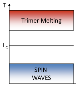
Figure 2: (Color online) The phase diagram of the trimer system as a function of temperature $T$, as discussed in the text. Long range magnetic order occurs at $T_{c}$. Trimer formation occurs over the regime for which $T$ is of order $J$.

The Hamiltonian for the system of spins 1/2 which we treat is written as

$${\cal H} = \sum_{\langle ij\rangle}J_{ij}{\bf S}_{i}\cdot{\bf S}_{j}\ ,$$ (1)

where $\langle ij\rangle$ indicates that the sum is over pairs of nearest neighbors on the Kagomé lattice. Here we neglect exchange anisotropy, in particular we do not include the Dzialoshinskii-Moriya [DM1, ; DM2, ] interaction, which can be the dominant anisotropic interaction between spins.[DM3, ; DM4, ] The values of the $J$’s are defined in Fig. 1 where the intra-trimer interaction $J$ is assumed to be dominant. We will work to leading order in $j/J$ or $k/J$ which are assumed to be of order $x<<1$. Thus the expansion parameter $x$ characterizes the ratio of inter-trimer to intra-trimer interactions. When inter-trimer interactions are turned on, the spectrum of discrete energy levels of isolated trimers gets broadened into a band of wavelike excitations, just as happens for atomic energy levels when placed in a solid.

For this calculation we obviously need the exact eigenfunctions and eigenvalues of the trimer Hamiltonian

$${\cal H}_{\rm T} = J{\bf S}_{a}\cdot{\bf S}_{b}+J{\bf S}_{b}\cdot{\bf S}_{c}\ ,$$ (2)

where the spins within a trimer are labeled as in Fig. 1. The total spin $\cal S$ is a good quantum number and assumes the values 3/2 and 1/2. The four states ${\cal S}=3/2$ are degenerate eigenstates of ${\cal H}_{\rm T}$ with eigenvalue $J/2$. The remaining four eigenstates form two ${\cal S}=1/2$ doublets. The eigenstates and eigenvalues of ${\cal H}_{\rm T}$ are listed in Table I. In the next section we consider the ground state manifold and in the following sections we consider excitations to the higher manifolds centered at energy $J$ and $3J/2$ above the ground state.

Before starting the calculation we should discuss when the trimer limit we consider is appropriate. First of all, our results show the obvious fact that when the trimers interact with one another, the single-trimer energy levels get broadened into a band. Clearly, a condition for treating isolated trimers as a starting point, would be that this broadening is small enough that the bands are separated and qualitatively retain their identity from the noninteracting limit. But additionally, in view of the fact that the trimers will be shown to act as spin 1/2’s, one could question whether this calculation improves the treatment of quantum zero-point which can be severe for $S=1/2$. The following qualitative estimate indicates why the trimer calculation can be useful. Let us consider excitation relative to the Néel state in which spins are aligned along the $z$-axis. The perturbation which creates zero-point motion comes from terms like $J_{ij}S_{-}(i)S_{+}(j)/2$, where the subscript labels the Cartesian component of spin and the largest such terms are those for which sites $i$ and $j$ are inside the same trimer. This perturbation $V$ connects the ground state to a state with excitation energy $E=2zJS$, where $z$, the number of nearest neighbors should be taken to be 1 or 2 because for each site there are only 1 or 2 strongly coupled neighbors. Thus $V/E\approx 1/2$. In contrast, when this type of calculation is repeated for the trimer state $z$ is now 4, the number of trimer-trimer nearest neighbors. Also, perturbative corrections to a system of isolated trimers are of order $V/E=j/J$, where $j$ is one of the inter-trimer interactions. So zero point corrections are less important for the trimer analog of the Néel state than for the usual Néel state in the limit when $j/J$ is small.

III Ground-State Excitations

We first consider the $2^{N}$-fold degenerate manifold of $N$ trimers when intertrimer interactions are turned off, so that each trimer has energy $-J$. To implement degenerate perturbation theory when intertrimer interactions are turned on, it is convenient to map this manifold of states onto the $2^{N}$ states associated with a system of $N$ pseudospin 1/2 operators, such that the pseudospin operator of each trimer is simply the total ground state spin operators ${\cal S}$ of that trimer. For the trimer at position ${\bf R}$ we denote this pseudospin operator as ${\mbox{\boldmath{$\sigma$}}}({\bf R})$. Then, any operator within the ground manifold can be expressed in terms of products of one or more ${\mbox{\boldmath{$\sigma$}}}({\bf R})$. We then use the wavefunctions in Table I to express matrix elements of spin operators for individual sites within the trimer at ${\bf R}$ to ${\mbox{\boldmath{$\sigma$}}}({\bf R})$. For this purpose we label the three spins within a trimer as $a$, $b$, and $c$ as in Fig. 1. Using Table 1 we note that for an A trimer (for which ${\mbox{\boldmath{$\sigma$}}}_{z}=1/2$), the expectation value of the $z$-component of the $k$th spin in the ground state of the trimer denoted $S_{z}(k)$ (where $k=a,b,c$) is

$$S_{z}(a) = 1/3\ ,\ \ S_{z}(b)=-1/6\ ,\ \ S_{z}(c)=1/3\ .$$ (3)

This result reflects the fact that the central spin partakes of spin fluctuations with its two neighbors inside the trimer whereas an end spin of the trimer has only one neighbor with which to fluctuate. Below we will discuss the experimental consequences of this result. In fact, the Wigner-Eckart theoremROSE indicates that we have, as an operator equality within the ground manifold, that

$${\bf S}(a;{\bf R}) = 2{\mbox{\boldmath{$\sigma$}}}({\bf R})/3\ ,$$

$${\bf S}(b;{\bf R}) = -{\mbox{\boldmath{$\sigma$}}}({\bf R})/3\ ,$$

$${\bf S}(c;{\bf R}) = 2{\mbox{\boldmath{$\sigma$}}}({\bf R})/3\ ,$$ (4)

where ${\bf S}(k;{\bf R})$ is the operator for the $k$th spin in the trimer whose center is at ${\bf R}$ and, as we have said, the pseudo-spin operator is identified as the total spin of the trimer:

$${\mbox{\boldmath{$\sigma$}}}({\bf R})=\sum_{k=a}^{c}{\bf S}(k;{\bf R})\ .$$ (5)

These equalities make it a trivial matter to write the inter-trimer interactions in terms of the $\sigma$’s. So we see, even without calculation, that the low-energy spectrum of the trimer system is identical to that of a system in which each trimer is replaced by an ordinary spin 1/2.

Table 1: Eigenvectors $\psi_{n}$ and eigenvalues $\lambda_{n}$ of ${\cal H}_{\rm T}$. The states specified by three vertical arrows give the values of $S_{z}$ for spins $a$, $b$, and $c$ (reading from left to right), as shown in Fig. 1. The index $n$ is only used to label excited states.

$n$	${\cal S}$	${\cal S}_{z}$	$\psi_{n}$	$\lambda_{n}$
$6$	$\frac{3}{2}$	$\frac{3}{2}$	$|\uparrow,\uparrow,\uparrow\rangle$	$J/2$
$5$	$\frac{3}{2}$	$\frac{1}{2}$	$[|\uparrow,\uparrow,\downarrow\rangle+|\uparrow,\downarrow,\uparrow\rangle+|\downarrow,\uparrow,\uparrow\rangle]/\sqrt{3}$	$J/2$
$4$	$\frac{3}{2}$	$-\frac{1}{2}$	$[|\uparrow,\downarrow,\downarrow\rangle+|\downarrow,\uparrow,\downarrow\rangle+|\downarrow,\downarrow,\uparrow\rangle]/\sqrt{3}$	$J/2$
$3$	$\frac{3}{2}$	$-\frac{3}{2}$	$|\downarrow,\downarrow,\downarrow\rangle$	$J/2$
$2$	$\frac{1}{2}$	$\frac{1}{2}$	$[|\uparrow,\uparrow,\downarrow\rangle-|\downarrow,\uparrow,\uparrow\rangle]/\sqrt{2}$	$0$
$1$	$\frac{1}{2}$	$-\frac{1}{2}$	$[|\uparrow,\downarrow,\downarrow\rangle-|\downarrow,\downarrow,\uparrow\rangle]/\sqrt{2}$	$0$
	$\frac{1}{2}$	$\frac{1}{2}$	$[|\uparrow,\uparrow,\downarrow\rangle-2|\uparrow,\downarrow,\uparrow\rangle+|\downarrow,\uparrow,\uparrow\rangle]/\sqrt{6}$	$-J$
	$\frac{1}{2}$	$-\frac{1}{2}$	$[-|\uparrow,\downarrow,\downarrow\rangle+2|\downarrow,\uparrow,\downarrow\rangle-|\downarrow,\downarrow,\uparrow\rangle]/\sqrt{6}$	$-J$

We now consider the ground state and elementary excitations of the system when weak interactions between trimers are included. We will assume that all end-to-end exchange interactions between nearest neighbor trimers assume a common value $k$ and those between the end of one trimer and the center of its nearest neighbor assume a common value $j$ as shown in Fig. 1. This symmetry we have imposed makes the calculations algebraiclly simple. If the intra-trimer and inter-trimer interactions have no special symmetry, the calculations becomes algebraically more complicated but are conceptually no more difficult. So here we give results only for the model of Fig. 1.

We now construct the effective Hamiltonian within the ground state manifold. Consider the interaction $V(A,B)$ between trimers A and B. We use the Wigner-Eckart theorem to express the spin operators in terms of the pseudo or total spin of the trimer, as done in Eq. (4). Then one sees that $V(A,B)$ within the ground manifold is given by

$$V(A,B) = [{\mbox{\boldmath{$\sigma$}}}(A)\cdot{\mbox{\boldmath{$\sigma$}}}(B)][4k-2j]/9$$ (6)

$$\equiv {\cal J}[{\mbox{\boldmath{$\sigma$}}}(A)\cdot{\mbox{\boldmath{$\sigma$}}}(B)]\ ,$$

where

$${\cal J} = (4k-2j)/9\ .$$ (7)

One sees that the effective exchange interaction between two nearest neighboring trimers is antiferromagnetic if $2k-j>0$ and is ferromagnetic if $2k-j<0$.PB Thus the trimer-trimer interaction can be ferromagnetic even if all the spin-spin interactions are positive (antiferromagnetic) providing $j>2k$. These configurations are shown in Fig. 3. The elementary excitations within the ground manifold are those of a rectangular centered lattice. Then, if the trimers are antiferromagnetically coupled, standard spin-wave theorySWAVE gives the doubly degenerate spin-wave energy $\omega_{\pm}({\bf q})$ as a function of wave vector ${\bf q}$, for $-\pi/(2s)<q_{y}<\pi/(2s)$ and $-\pi/(2\sqrt{3}s)<q_{z}<\pi/(2\sqrt{3}s)$, as

$$\omega({\bf q}) = z{\cal J}S\sqrt{1-\gamma({\bf q})^{2}}\ ,$$ (8)

where $z=4$ is the number of nearest neighbors, $S=1/2$, and

$$\gamma({\bf q}) = (1/z)\sum_{\mbox{\boldmath{$\delta$}}}\exp(i{\bf q}\cdot{\mbox{\boldmath{$\delta$}}})$$ (9)

$$= \cos(sq_{y})\cos(\sqrt{3}sq_{z})\ .$$

Here $\delta$ is summed over nearest neighbor vectors between trimers and $s$ is the nearest neighbor separation in the Kagomé lattice, as in Fig. 1. If the trimers are ferromagnetically coupled, then one has two nondegenerate modes whose energy is given by

$$\omega_{\pm}({\bf q}) = z|{\cal J}|S[1\pm\gamma({\bf q})]\ .$$ (10)

Here (in Fig. 4) and below we give results for $J=1$ for the antiferromagnetic configuration of trimers with $j=0.15$ and $k=0.2$ and for the ferromagnetic configuration with $j=0.2$ and $k=0.05$. Note that transverse ($+-$) modes of the antiferromagnetic configuration of trimers are doubly degenerate for all wave vectors. Also here and below note that the spectrum is always two fold degenerate for wave vectors on the face of the Brillouin zone [$k_{y}=\pi/(2s)$] due to the Kramers-like degeneracy from the two-fold screw axis.[HEINE, ]

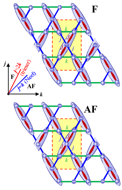
Figure 3: (Color online) As Fig. 1, the ferromagnetic (F) and antiferromagnetic (AF) arrangement of trimers, with spin orientation indicated by $+$ or $-$. The inset graph shows the phase diagram of the trimer system in the $j$-$k$ plane. The F-AF phase boundary based on the Néel state is at $j=k$ and according to the trimer calculation is at $j=2k$. The latter calculation is more nearly correct when $J$ is large compared to $j$ or $k$, whereas the former is more accurate when $J$ is not large compared to $j$ and $k$.

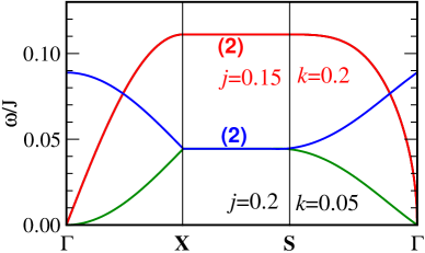
Figure 4: (Color online) Spectrum of excitation energy, $\omega({\bf q})$ within the ground manifold for wave vectors in special directions. Here and below we plot the spectra for $J=1$ for wavevectors on the lines joining $\Gamma$ and ${\bf X}$, ${\bf X}$ and ${\bf S}$, and ${\bf S}$ and $\Gamma$, where $\Gamma=(0,0)$, $X=[\pi/(2s),0)$, and $S=[\pi/(2s),\pi/(2\sqrt{3}s)$. For ($j=0.15$, $k=0.2$) one has a ferro configuration of trimers and for ($j=0.2$, $k=0.05$) one has an antiferro configuration of trimers. The modes shown here appear only in the transverse ($+-$) response function. Modes are nondegenerate unless labeled “(2)” to indicate a two-fold degeneracy.

IV Exciton Spectrum

Now we turn to the excitations out of the ground state manifold.

IV.1 Manifold at Energy $J$ for the Antiferro Configuration

Here we treat the case of antiferromagnetic coupling ( ${\cal J}>0$). The situation for this manifold is more complicated than that for the ground manifold. For the ground manifold we could develop degenerate perturbation theory for the manifold of $2^{N}$ states of the system of $N$ trimers in which each trimer independently occupies one of its two degenerate ground states. The result was embodied in an effective Hamiltonian in which the interactions between nearest neighboring trimers was given by Eq. (7). For excitations near energy $J$ we might consider the manifold of states in which one trimer occupies one of the excited states of Table I and all the other $N-1$ trimers are distributed over the two degenerate ground states. Strictly speaking this involves the solution to a many-body problem for the states of a spin excitation within the ground manifold and an exciton at excitation energy $J$ or $3J/2$. We will not treat this system with this degree of sophistication. Instead, we will treat the manifold of excited states at relative energy $J$ or $3J/2$ when all the background trimers are confined to their broken symmetry ground state. Thus our treatment is limited to the range of temperature $T$ for which $kT\ll{\cal J}$. We therefore introduce operators $a_{n}^{\dagger}({\bf R})$ which take the trimer at ${\bf R}$ from its ground state to its $n$th excited state, where the labeling of sites is given in the first column of Table 1. The Hamiltonian which describes the manifold at energy $J$ is

$${\cal H}(J) = J\sum_{\bf R}\sum_{n=1}^{2}n_{n}({\bf R})+V(J)\ ,$$ (11)

where ${\bf R}$ is summed over trimer sites and $n_{n}=a_{n}^{\dagger}a_{n}$. Within the manifold near energy $J$ the term in Eq. (11) proportional to $J$ is a constant and the nature of the band states is determined solely by the perturbation $V(J)$, which contains only terms proportional to $j$ or $k$. To obtain results to leading order in the expansion parameter $x$, the perturbation $V(J)$ is thus restricted to terms which conserve the unperturbed energy $J$. Accordingly, the most general such form of $V(J)$ is

$$V(J) = \sum_{{\bf R},{\bf R}^{\prime}}\sum_{n,m=1}^{2}c_{nm}({\bf R},{\bf R}^{\prime})a_{n}^{\dagger}({\bf R})a_{m}({\bf R}^{\prime})+...$$ (12)

where the dots denote terms containing $p$ creation operators (all with indices in the range 1,2) and $p$ analogous destruction operators. Since we only consider nearest-neighbor interactions, we set

$${\bf R}^{\prime}={\bf R}_{n}={\bf R}+{\mbox{\boldmath{$\delta$}}}_{n}\ ,$$ (13)

where ${\mbox{\boldmath{$\delta$}}}_{n}$ are the nearest neighbor intertrimer displacements shown in Fig. 1:

$${\mbox{\boldmath{$\delta$}}}_{1} = -s\hat{j}-\sqrt{3}s\hat{k}\ ,\hskip 21.68121pt{\mbox{\boldmath{$\delta$}}}_{2}=s\hat{j}-\sqrt{3}s\hat{k}$$

$${\mbox{\boldmath{$\delta$}}}_{3} = s\hat{j}+\sqrt{3}s\hat{k},\hskip 21.68121pt{\mbox{\boldmath{$\delta$}}}_{4}=-s\hat{j}+\sqrt{3}s\hat{k}\ .$$ (14)

The effect of these $2p$th order terms in Eq. (12) on the mode energies is proportional to the $(p-1)$th power of the density of excitations. Since we assume that $kT\ll J$, this density is small and we keep only the terms with $p=1$. In addition we ignore the kinematic constraint which allows one to map the finite number of trimer states onto the infinite number of bosonic states.[FJD, ] The discussion for the band at energy $3J/2$ is completely analogous to that for energy $J$ and the analogous result holds for that case. So the band states are completely determined by the matrix $c_{n,m}({\bf R},{\bf R}^{\prime})$, or, as will shall see, by its Fourier transform which is a 4$\times$4 matrix for the band at energy $J$ and an 8$\times$8 matrix for the band at energy $3J/2$. To explicitly determine $V(J)$ we must express the spin Hamiltonian in terms of the creation and annihilation operators of Eq. (12). The spin interaction between the $k$th spin of an up trimer at ${\bf R}$ and the $k^{\prime}$th spin of a down trimer at ${\bf R}^{\prime}$ is

$${\bf S}(k;{\bf R})\cdot{\bf S}(k^{\prime};{\bf R}^{\prime})=S_{z}(k;{\bf R})S_{z}(k^{\prime};{\bf R}^{\prime})$$

$$\ \ +[S_{+}(k;{\bf R})S_{-}(k^{\prime};{\bf R}^{\prime})+S_{-}(k;{\bf R})S_{+}(k^{\prime};{\bf R}^{\prime})]/2\ ,$$ (15)

Since $S_{+}$ and $S_{-}$ each involve at least one creation or annihilation operator, to construct the boson Hamiltonian, we need only keep terms in these operators which are linear in the creation or destruction operators. In contrast, since $S_{z}$ has a nonzero value in the ground state, we also need to keep terms in $S_{z}$ which involve one creation operator and one destruction operator within the band. These considerations will be used implicitly below to limit the complexity of the mapping from spins to bosons.

For the case of an “up” trimer at ${\bf R}$ (one whose ground state has ${\cal S}_{z}=1/2$ and which we refer to as an “A” trimer) we find (keeping only terms linear in the boson operators) that

$$S_{-}(a;{\bf R}) = a_{1}^{\dagger}({\bf R})/\sqrt{3}-a_{4}^{\dagger}({\bf R})/\sqrt{18}$$

$$+a_{6}({\bf R})/\sqrt{6}$$

$$S_{-}(b;{\bf R}) = 2a_{4}^{\dagger}({\bf R})/\sqrt{18}-2a_{6}({\bf R})/\sqrt{6}$$

$$S_{-}(c;{\bf R}) = -a_{1}^{\dagger}({\bf R})/\sqrt{3}-a_{4}^{\dagger}({\bf R})/\sqrt{18}$$ (16)

$$\ \ +a_{6}({\bf R})/\sqrt{6}\ .$$

The expression for $S_{+}(k,{\bf R})$ are obtained by Hermitian conjugation. To determine the bosonic equivalent of $S_{z}$ we write

$$S_{z} =a_{0}+\sum_{nm}a_{nm}a_{n}^{\dagger}a_{m}\ .$$ (17)

To determine the coefficients we require that the two representations lead to the same matrix elements. Thus if 0 labels the ground state (i. e. whichever of the $-J$ states of the trimer is the ground state), then, by taking matrix elements of both sides of Eq. (17) we get

$$a_{0} = \langle 0|S_{z}|0\rangle\ ,\ \ \ \ a_{n,m}=\langle n|S_{z}|m\rangle\ ,\ \ \ n\not=m$$

$$a_{0} + a_{n,n}=\langle n|S_{z}|n\rangle\ ,\ \ \ n\not=0\ .$$ (18)

So for diagonal elements we must remember to subtract off the ground state value when identifying the bosonic matrix elements $a_{nn}$. Thus

$$S_{z}(a;{\bf R})=1/3+a_{2}^{\dagger}({\bf R})/\sqrt{12}-a_{5}^{\dagger}({\bf R})/\sqrt{18}$$

$$+a_{2}({\bf R})/\sqrt{12}-a_{5}({\bf R})/\sqrt{18}-[2n_{1}({\bf R})+2n_{2}({\bf R})$$

$$+5n_{3}({\bf R})+3n_{4}({\bf R})+n_{5}({\bf R})-n_{6}({\bf R})]/6\ ,$$

$$S_{z}(b;{\bf R})=-1/6+2a_{5}^{\dagger}({\bf R})/\sqrt{18}$$

$$+2a_{5}({\bf R})/\sqrt{18}-n_{1}({\bf R})/3+2n_{2}({\bf R})-n_{3}({\bf R})/3$$

$$+n_{5}({\bf R})/3+2n_{6}({\bf R})/3\ ,$$

$$S_{z}(c;{\bf R})=1/3-a_{2}^{\dagger}({\bf R})/\sqrt{12}-a_{5}^{\dagger}({\bf R})/\sqrt{18}$$

$$-a_{2}({\bf R})/\sqrt{12}-a_{5}({\bf R})/\sqrt{18}-[2n_{1}({\bf R})+2n_{2}({\bf R})$$

$$+5n_{3}({\bf R})+3n_{4}({\bf R})+n_{5}({\bf R})-n_{6}({\bf R})\ .$$ (19)

Here we needed to keep $a_{p}^{+}a_{p}\equiv n_{p}$ terms in view of Eqs. (15) and (18).

For the case of a “down” trimer (one whose ground state has ${\cal S}_{z}=-1/2$ at ${\bf R}$ and which we refer to as a “B” trimer) we similarly find that

$$S_{+}(a;{\bf R})=a_{2}^{\dagger}({\bf R})/\sqrt{3}+a_{5}^{\dagger}({\bf R})/\sqrt{18}$$

$$-a_{3}({\bf R})/\sqrt{6}$$

$$S_{+}(b;{\bf R})=-2a_{5}^{\dagger}({\bf R})/\sqrt{18}+2a_{3}({\bf R})/\sqrt{6}$$

$$S_{+}(c;{\bf R})=-a_{2}^{\dagger}({\bf R})/\sqrt{3}+a_{5}^{\dagger}({\bf R})/\sqrt{18}$$

$$\ \ -a_{3}({\bf R})/\sqrt{6}\ ,$$

$$S_{z}(a;{\bf R})=-1/3-a_{1}^{\dagger}({\bf R})/\sqrt{12}$$

$$-a_{4}^{\dagger}({\bf R})/\sqrt{18}-a_{1}({\bf R})/\sqrt{12}-a_{4}({\bf R})/\sqrt{18}$$

$$+n_{1}({\bf R})/3+n_{2}({\bf R})/3-n_{3}({\bf R})/6$$

$$+n_{4}({\bf R})/6+n_{5}({\bf R})/2+5n_{6}({\bf R})/6\ ,$$

$$S_{z}(b;{\bf R})=1/6+2a_{4}^{\dagger}({\bf R})/\sqrt{18}$$

$$+2a_{4}({\bf R})/\sqrt{18}-2n_{1}({\bf R})/3+n_{2}({\bf R})/3$$

$$-2n_{3}({\bf R})/3-n_{4}({\bf R})/3+n_{6}({\bf R})/3\ ,$$

$$S_{z}(c;{\bf R})=-1/3+a_{1}^{\dagger}({\bf R})/\sqrt{12}$$

$$-a_{4}^{\dagger}({\bf R})/\sqrt{18}+a_{1}({\bf R})/\sqrt{12}-a_{4}({\bf R})/\sqrt{18}$$

$$+n_{1}({\bf R})/3+n_{2}({\bf R})/3-n_{3}({\bf R})/6$$

$$+n_{4}({\bf R})/6+n_{5}({\bf R})/2+5n_{6}({\bf R})/6\ .$$ (20)

The next step is to write the interaction between trimers in terms of boson operators. Since we treat here the case when the trimers are antiferromagnetically coupled, all interactions couple an up (A) trimer to a down (B) trimer. Since we treat only nearest neighbor interactions, we need consider only interactions between an up trimer at ${\bf R}$ and one of its four down neighbors at ${\bf R}\pm{\mbox{\boldmath{$\delta$}}}_{1}$ and ${\bf R}\pm{\mbox{\boldmath{$\delta$}}}_{2}$. For the excitations band near energy $J$ the boson Hamiltonian is obtained in Appendix A. We define the Fourier transformed variables as

$$a_{n,A}^{\dagger}({\bf k})=N^{-1/2}\sum_{{\bf R}\in{\rm A}}e^{i{\bf k}\cdot{\bf R}}a_{n}^{\dagger}({\bf R})$$

$$a_{n,B}^{\dagger}({\bf k})=N^{-1/2}\sum_{{\bf R}\in{\rm B}}e^{i{\bf k}\cdot{\bf R}}a_{n}^{\dagger}({\bf R})\ ,$$ (21)

where $N$ is the total number of unit cells in the system. The quadratic Hamiltonian is of the canonical form: ${\cal H}=\sum_{\bf q}{\cal H}_{\bf q}$, where ${\bf q}$ is the wave vector and because we need consider only terms which conserve the unperturbed energy $J$,

$${\cal H}_{\bf q} = \sum_{n,n^{\prime};\tau,\tau^{\prime}}A_{st}({\bf q})a_{s}^{\dagger}({\bf q})a_{t}({\bf q})\ ,$$ (22)

where $s\equiv(n,\tau)$ and $t\equiv(n^{\prime},\tau^{\prime})$.

According to Table 1, excitations near energy $J$ involve states 1 and 2 of the two spins in the unit cell, whereas excitations near energy $3J/2$ involve states 3, 4, 5, snf 6 of the two spins in the unit cell. For excitations near energy $J$ we write

$${\bf A} = J{\cal I}+k{\bf A}_{k}+j{\bf A}_{j}\ ,$$ (23)

where ${\cal I}$ is the $4\times 4$ unit matrix and Eq. (154) of Appendix A implies that

$${\bf A}_{k} = \frac{1}{9}\left[\begin{array}[]{c c c c}4&0&0&0\\ 0&4&3\gamma({\bf q})&0\\ 0&3\gamma({\bf q})&4&0\\ 0&0&0&4\\ \end{array}\right]\ ,$$ (28)

and

$${\bf A}_{j} = \frac{1}{9}\left[\begin{array}[]{c c c c}1&0&0&0\\ 0&-5&0&0\\ 0&0&-5&0\\ 0&0&0&1\\ \end{array}\right]\ .$$ (33)

The rows and columns of the matrices ${\bf A}$ are labeled in the order $(1,A)$, $(2,A)$, $(1,B)$, $(2,B)$.

Thus the creation operators for the normal modes are $a_{1,A}({\bf q})^{\dagger}$, $a_{2,B}({\bf q})^{\dagger}$, and

$$\rho_{\pm}^{\dagger} = [a_{1,B}({\bf q})^{\dagger}\pm a_{2,A}({\bf q})^{\dagger}]/\sqrt{2}\ ,$$ (34)

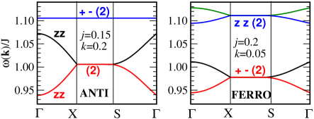
Figure 5: (Color online) As Fig. 4, but for excitations in the manifold near energy $J$ for the antiferro (left) and ferro (right) configurations. The curve labeled ”$+-$” indicates the energy in the transverse ($+-$) response function and those labeled ”zz” are the energies in the longitudinal ($zz$) response function. The numbers in parentheses indicate the degeneracy of the mode.

with associated eigenenergies

$$\omega_{1A}({\bf q}) = \omega_{2B}({\bf q})=J+(4k+j)/9$$ (35)

and

$$\omega_{\pm}({\bf q}) = J+(4k-5j)/9\pm(k/3)\gamma({\bf q})\ .$$ (36)

These results are shown in Fig. 5. For an A (up) trimer $a_{1,A}^{\dagger}$ corresponds to $S_{-}$ and $a_{2,B}^{\dagger}$ corresponds to $S_{+}$ for a B (down) trimer. So these operators create transverse excitations and similarly one sees that $\rho_{\pm}^{\dagger}$ create a longitudinal excitation. It may be surprising that, unlike for a Néel antiferromagnet, the longitudinal excitations exhibit dispersion, but the transverse ones do not. However, note that for a Néel antiferromagnet the dispersion comes from $a^{\dagger}a^{\dagger}$ terms which here are eliminated since they do not conserve the large unerperturbed energy.

IV.2 Manifold at Energy $J$ for the Ferro Configuration

The calculations for the ferro configuration (in which all trimers start in their ‘up’ ground state) are similar and are done in Appendix C. In terms of Fourier transformed variables Eq. (223) implies, in the notation of Eq. (23), that

$${\bf A}_{j} = \frac{1}{9}\left[\begin{array}[]{c c c c}-1&0&0&0\\ 0&5&0&0\\ 0&0&-1&0\\ 0&0&0&5\\ \end{array}\right]\ ,$$ (41)

$${\bf A}_{k} = \frac{1}{9}\left[\begin{array}[]{c c c c}-4&0&-6\gamma({\bf q})&0\\ 0&-4&0&-3\gamma({\bf q})\\ -6\gamma({\bf q})&0&-4&0\\ 0&-3\gamma({\bf q})&0&-4\\ \end{array}\right]\ ,$$ (46)

where the rows and columns are labeled in the order $(A,1)$, $(A,2)$, $(B,1)$, $(B,2)$. The eigenvalues give the mode energies:

$$\omega_{1,2} = J-j/9-4k/9\pm 2k\gamma({\bf q})/3$$

$$\omega_{3,4} = J+5j/9-4k/9\pm k\gamma({\bf q})/3\ .$$ (48)

These mode energies are shown for high symmetry wave vectors in Fig. 5. Since $a_{A1}^{\dagger}$ or $a_{B1}^{\dagger}$ connects the up ground state to a state with ${\cal S}_{z}=-1/2$, these operators correspond to an $S_{-}$. Thus we identify $\omega_{1,2}$ as energies of transverse excitations and $\omega_{3,4}$ as energies of longitudinal excitations as indicated in Fig. 5.

IV.3 Manifold at Energy $3J$/2 for the Antiferro Configuration

Here we adopt the same simplified approximation in which trimers not in excited states remain in their Néel state. Then, to leading order in the inter-trimer interactions, we only keep terms which are quadratic in the variables 3, 4, 5, and 5 and which conserve the total number of excitations. Thus analagously to Eq. (11) we write

$${\cal H}(3J/2) = (3J/2)\sum_{\bf R}\sum_{n=3}^{6}n_{n}({\bf R})+V(3J/2)\ ,$$ (49)

The evaluation of $V(3J/2)$ for the antiferro configuration is given in Eq. (192) of Appendix B. In the notation of Eq. (23), where we label the rows and columns of the matrices in the order 3A, 6B, 4A, 3B, 5A, 4B, 6A, 5B, that result implies that

$${\bf A}_{k} = \frac{1}{9}\left[\begin{array}[]{c c c c c c c c}10&0&0&0&0&0&0&0\\ 0&10&0&0&0&0&0&0\\ 0&0&6&X&0&0&0&0\\ 0&0&X&-2&0&0&0&0\\ 0&0&0&0&2&Y&0&0\\ 0&0&0&0&Y&2&0&0\\ 0&0&0&0&0&0&-2&X\\ 0&0&0&0&0&0&X&6\\ \end{array}\right]\ ,$$ (58)

$${\bf A}_{j} = \frac{1}{18}\left[\begin{array}[]{c c c c c c c c}-1&0&0&0&0&0&0&0\\ 0&-1&0&0&0&0&0&0\\ 0&0&-3&T&0&0&0&0\\ 0&0&T&-7&0&0&0&0\\ 0&0&0&0&-5&U&0&0\\ 0&0&0&0&U&-5&0&0\\ 0&0&0&0&0&0&-7&T\\ 0&0&0&0&0&0&T&-3\\ \end{array}\right]\ ,$$ (67)

where

$$T = -4\sqrt{3}\gamma({\bf q})\ ,\ \ \ U=-8\gamma({\bf q})\ ,$$

$$X = \sqrt{3}\gamma({\bf q})\ ,\ \ \ Y=2\gamma({\bf q})\ .$$ (68)

Thus we have the mode energies, with their degeneracies in parentheses:

$$\omega_{1} = 3J/2+10k/9-j/18\ (2)\ ,$$

$$\omega_{2,3} = 3J/2+2k/9-5j/18\pm(4j-2k)\gamma({\bf q})/9\ \ (1)$$

$$\omega_{4,5} = 3J/2+2k/9-5j/18$$ (69)

$$\pm \sqrt{(4k+j)^{2}+3(k-2j)^{2}\gamma({\bf q})^{2}}/9\ \ (2)\ .$$

We determine the polarization of the modes as follows. The mode $\omega_{1}$ involves state 3A which has ${\cal S}_{A,z}=-3/2$ or state 6B which has ${\cal S}_{B,z}=3/2$ and is therefore not accessible via a single spin operator from the ${\cal S}_{A,z}=1/2$, ${\cal S}_{B,z}=-1/2$ ground state. The modes $\omega_{2}$ and $\omega_{3}$ arise from states 5A and 4B. State 5A has ${\cal S}_{A,z}=1/2$, which is activated from the ${\cal S}_{A,z}=1/2$ ground state by an ${\cal S}_{A,z}$ operator and state 4B has ${\cal S}_{B,z}=-1/2$ which is activated from the ${\cal S}_{B,z}=-1/2$ ground state by an ${\cal S}_{B,z}$ operator. The modes $\omega_{4}$ and $\omega_{5}$ arise from states 4A, 3B, 6A, or 5B. State 4A has ${\cal S}_{A,z}=-1/2$, which is activated by an ${\cal S}_{A,-}$ operator and state 5B has ${\cal S}_{B,z}=1/2$ which is activated by an ${\cal S}_{B,+}$ operator. States 3B or 6A lead to similar results. These modes (with their polarizations) are shown in Fig. 6.

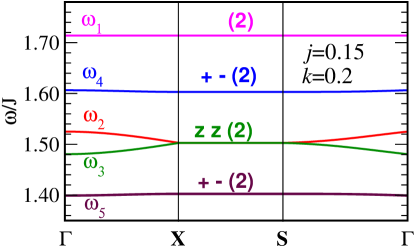
Figure 6: (Color online) As Fig. 5, but for modes near energy $3J/2$ for the antiferro configuration. The highest-energy mode is not accessible in linear (in ${\bf S}$) response theory.

IV.4 Manifold at energy $3J$/2 for Ferro Configuration

The result of the calculation of $V(3J/2)$ for the ferro configuration is given in Eq. (LABEL:EQD7) of Appendix D, which implies, in the notation of Eq. (23), that

$${\bf A}_{k} = \frac{1}{9}\left[\begin{array}[]{c c c c c c c c}-10&0&0&0&0&0&0&0\\ 0&-6&0&0&0&1&0&0\\ 0&0&-2&0&0&0&2&0\\ 0&0&0&2&0&0&0&3\\ 0&0&0&0&-10&0&0&0\\ 0&1&0&0&0&-6&0&0\\ 0&0&2&0&0&0&-2&0\\ 0&0&0&3&0&0&0&2\\ \end{array}\right]\ ,$$ (78)

$${\bf A}_{j} = \frac{1}{18}\left[\begin{array}[]{c c c c c c c c}1&0&0&0&0&0&0&0\\ 0&3&0&0&0&4&0&0\\ 0&0&5&0&0&0&8&0\\ 0&0&0&7&0&0&0&12\\ 0&0&0&0&1&0&0&0\\ 0&4&0&0&0&3&0&0\\ 0&0&8&0&0&0&5&0\\ 0&0&0&12&0&0&0&7\\ \end{array}\right]\ ,$$ (87)

where the rows and column are labeled in the order 3A, 4A, 5A, 6A, 3B, 4B, 5B, 6B. We thereby find the mode energies to be

$$\omega_{1,2} = 1.5J+\frac{j-20k}{18}\ ,$$

$$\omega_{3,4} = 1.5J+\frac{3j-12k}{18}\pm\frac{k-2j}{9}\gamma({\bf q})\ ,$$

$$\omega_{5,6} = 1.5J+\frac{5j-4k}{18}\pm\frac{2k-4j}{9}\gamma({\bf q})\ ,$$

$$\omega_{7,8} = 1.5J+\frac{7j+4k}{18}\pm\frac{k-2j}{3}\gamma({\bf q})\ .$$ (88)

The determination of the polarization of the mode is done as we did for the modes of Eq. (69). The results are shown in Fig. 7.

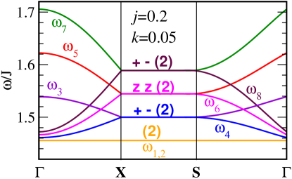
Figure 7: (Color online) As Fig. 5, but for excitations in the manifold near energy $1.5J$ for the ferro configuration from Eq. (88). The lowest-energy mode is not accessible in linear (in ${\bf S}$) response theory.

V NÉEL SPIN WAVES

In this section we compare the results obtained above with those from ordinary spin-wave theory. In Fig. 8 we show the 6 branches of transverse excitations from the Néel ground state.

Note that apart from the lowest manifold, the two approaches lead to quite different spectra. As we showed above, the lowest manifold of trimer excitations is obtained by an exact mapping onto a Néel spin spectrum. One sees that for the anti configuration the energy scale of the lowest branch of spin waves is significantly larger for the trimer approach than for the Néel approach. This is because the trimer approach takes better account of quantum zero point motion that does the Néel approach. It is well known that zero point fluctuations tend to increase the spin-wave energies. This is shown by exact calaculations for one dimensional spin chains[CHAINS, ] and by perturbative calculations for three dimensional systems.[PERT, ] In contrast, for the ferro configuration the opposite effect occurs because the energies are proportional to the spin magnitudes.

Figure 8: (Color online) As Fig. 4. Néel (transverse) spin-wave spectrum for the anti (left) and ferro (right) configurations. Note that the two-fold degeneracy of the antiferromagnetic spectrum is broken along the low symmetry ${\bf S}$-$\Gamma$ line.

VI NEUTRON DIFFRACTION

Some aspects of neutron diffraction have been discussed by Furrer et al.FURRER1 and by Qiu et al.CB Here we discuss briefly the difference between the diffraction spectrum of the trimer system and that of the associated Néel state. The elastic magnetic scattering intensity is proportional to

$$\frac{d\sigma}{d\Omega}\approx\sum_{{\bf G}}(|{\bf F}({\bf Q})|^{2}-|\hat{\bf Q}\cdot{\bf F}({\bf Q})|^{2})\delta({\bf Q}-{\bf G}),$$ (89)

where ${\bf G}$ is summed over all reciprocal lattice vectors and the magnetic vector structure factor ${\bf F}$ is

$${\bf F}({\bf Q})\approx\sum_{\tau}\langle{\bf S}_{\tau}\rangle e^{i{\bf Q}\cdot{\bf\tau}},$$ (90)

where ${\bf\tau}$ are the copper spin-positions given in Table 2 and $\langle{\bf S}_{\tau}\rangle$ is the thermal average of the spin at site ${\bf\tau}$. For the Néel model, we take the spin-values as 0.5 while for the trimer model it is 1/6 and 1/3 as shown in Table 2. To simplify the presentation we do not discuss the atomic form factor and the Debye-Waller factor. The magnetic elastic diffraction intensities (apart from the thermal and magnetic form factors) are summarized in Figure 9 for different collinear spin configurations along the crystal axes for both the trimer and Néel models, including AF and Ferro spin configurations. As expected, there are significant differences between the antiferro and ferro ordered trimer configurations. Also, for a given spin-configuration, the trimer model is significantly different than the Néel model. Due to smaller spin values in the trimer phase, the intenties are much weaker. Hence, observation of the magnetic Bragg peaks would be much more difficult in the trimer phase than for the Néel model. Other than this difference, there are other differences at various scattering angle and it may be possible to distinguish the Néel and trimer model experimentally. In Figure  9, we also show nuclear scattering, which has some overlap with the strongest magnetic peaks. The unique magnetic peaks are at low angle and there are only a few of them.

Table 2: Structure parameters[WILLS, ] (very similar results are given in Ref. ACTA, ) for the distorted Kagomé system Cu₂(OD)₃ClSHL1 ; SHL2 . Here $x$, $y$, and $z$ are the P2₁c fractional coordinates with respect to axes ${\bf a}=9.1056\AA$, ${\bf b}=6.8151\AA$, and ${\bf c}=11.829\AA$, with $\beta=30.825^{\rm o}$. We choose the P2₁c setting because the Kagomé plane is $x\approx 0$ in the this setting. The last column, S, shows the non-zero spin component in the trimer phase and is taken as along the $a-$, $b-$, and $c-$axis respectively in Figure9. For the Néel model, we set the spin magnitude to 0.5 instead of 1/3 and 1/6. The Cu₃ sites are in the triangular lattice planes which interleave the Kagomé planes, but our calculations do not include their moments.

Cu-sites	$x$	$y$	$z$	S
Cu1(1)	0	0	0	-1/6
Cu1(2)	0	1/2	1/2	1/6
Cu2(2)	0.0072	0.2658	0.2409	-1/3
Cu2(3)	0.9929	0.7658	0.2591	-1/3
Cu2(4)	0.9929	0.7342	0.7591	-1/3
Cu2(2)	0.0072	0.2342	0.7409	1/3
Cu3(1)	1/2	0	1/2	0
Cu3(2)	1/2	1/2	0	0

  

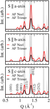
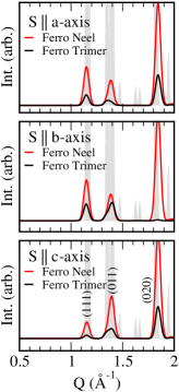
Figure 9: Elastic magnetic Bragg peaks for different spin alignments for trimer and Néel models for the AF (left) and Ferro (right) configurations, respectively. The gray lines in the background show the nuclear scattering.

VII INELASTIC SCATTERING SCATTERING CROSS SECTION

In this section we evaluate the inelastic cross section for the anti configuration at zero temperature. To do this we will construct the appropriate response functions, namely

$$\langle\langle A;B\rangle\rangle \equiv \sum_{n}\langle 0|A|n\rangle\langle n|B|0\rangle\delta(E_{n}-\hbar\omega)\ ,$$ (91)

where $|0\rangle$ denotes the ground state and the sum is over all states $|n\rangle$ with energy $E_{n}$ relative to the ground state. Here the operators $A$ and $B$ are proportional to the Fourier transforms of the spin operators. In particular we will need

$${\cal S}_{\alpha\beta}({\bf q},\omega) = \langle\langle S_{\alpha}({\bf q});S_{\beta}(-{\bf q})\rangle\rangle\ .$$ (92)

Thus

$${\cal S}_{+-}({\bf q},\omega) = \sum_{n}|\langle n|S_{-}({\bf q})|0\rangle|^{2}\delta(E_{n}-\hbar\omega)\ ,$$

$${\cal S}_{-+}({\bf q},\omega) = \sum_{n}|\langle n|S_{+}({\bf q})|0\rangle|^{2}\delta(E_{n}-\hbar\omega)\ ,$$

$${\cal S}_{zz}({\bf q},\omega) = \sum_{n}|\langle n|S_{z}({\bf q})|0\rangle|^{2}\delta(E_{n}-\hbar\omega)\ .$$ (93)

(We later set $\hbar=1$.) To analyze the single-magnon contributions to these quantities we need to relate the spin operators to the normal mode operators. Note that when we evaluate Eq. (93) at zero temperature, only contributions to the operator $S_{\beta}({\bf q})$ proportional to creation operators are nonzero. We will quote results for the transverse and longitudinal cross sections, given respectively by

$$I_{\rm trans}({\bf q},\omega) = {\cal S}_{+-}({\bf q},\omega)+{\cal S}_{-+}({\bf q},\omega),$$

$$I_{\rm long}({\bf q},\omega) = {\cal S}_{zz}({\bf q},\omega)\ .$$ (94)

In the calculations which follow we use the notation introduced in Sec. VI.

VII.0.1 GROUND-STATE EXCITATIONS

We first consider inelastic scattering from pseudo-spin waves. Accordingly, we discuss spin-wave theory for this situation. We express the pseudo-spin operators in terms of boson creation operators, $c_{A}^{\dagger}$ and $c_{B}^{\dagger}$ for the A (up) and B (down) trimers, respectively, as

$$\sigma_{z}(A) = 1/2-c_{A}^{\dagger}c_{A}$$

$$\sigma_{z}(B) = -1/2+c_{A}^{\dagger}c_{A}$$ (95)

and (with $\sigma_{\pm}=\sigma_{x}\pm i\sigma_{y}$)

$$\sigma_{-}(A) = c_{A}^{\dagger}\ ,\ \ \ \sigma_{-}(B)=c_{B}\ .$$ (96)

Then, following the standard spin-wave treatment for such a spin 1/2 system we write

$$c_{A}({\bf q}) = N^{-1/2}\sum_{\bf R\in A}e^{-i{\bf q}\cdot{\bf R}}c_{A}({\bf R})\ ,$$ (97)

and similarly for $c_{B}({\bf q})$, where ${\bf R}$ is summed over all the $N$ positions of A trimers. Then the boson Hamiltonian ${\cal H}\equiv\sum_{\bf q}{\cal H}_{\bf q}$ at quadratic order is

$${\cal H}_{\bf q} = 2{\cal J}\{c_{A}^{\dagger}({\bf q})c_{A}({\bf q})+c_{B}^{\dagger}(-{\bf q})c_{B}(-{\bf q})$$ (98)

$$+\gamma({\bf q})[c_{A}^{\dagger}({\bf q})c_{B}^{\dagger}(-{\bf q})+c_{A}({\bf q})c_{B}(-{\bf q})]\}\ .$$

Then the operators which create normal modes are $\rho^{\dagger}({\bf q})$ and $\eta^{\dagger}({\bf q})$, which are determined by

$$c_{A}^{\dagger}({\bf q}) = l({\bf q})\rho^{\dagger}({\bf q})-m({\bf q})\eta(-{\bf q})$$ (99)

and

$$c_{B}(-{\bf q}) = -m({\bf q})\rho^{\dagger}({\bf q})+l({\bf q})\eta(-{\bf q})\ ,$$ (100)

where

$$l({\bf q})^{2} = \frac{1+\epsilon({\bf q})}{2\epsilon({\bf q})}\ ,\ \ \ \ m({\bf q})^{2}=\frac{1-\epsilon({\bf q})}{2\epsilon({\bf q})}\ ,$$

$$l({\bf q})m({\bf q}) = \frac{\gamma({\bf q})}{2\epsilon({\bf q})}\ ,$$ (101)

with $\epsilon({\bf q})=[1-\gamma({\bf q})^{2}]^{1/2}$. Apart from the constant zero point energy one has

$${\cal H}=\sum_{\bf q}\omega({\bf q})[\rho^{\dagger}({\bf q})\rho({\bf q})+\eta^{\dagger}({\bf q})\eta({\bf q})]\ ,$$ (102)

where Eq. (8) is $\omega({\bf q})=2{\cal J}\epsilon({\bf q})$.

Using Eq. (4) we note that the Fourier transform of the spin operators is

$$S_{\alpha}({\bf q}) = N^{-1/2}\sum_{{\bf R}\in A}\sigma_{\alpha}({\bf R})e^{-i{\bf q}\cdot{\bf R}}\tau_{A}({\bf q})$$ (103)

$$\ +N^{-1/2}\sum_{{\bf R}\in B}\sigma_{\alpha}({\bf R})e^{-i{\bf q}\cdot{\bf R}}\tau_{B}({\bf q})\ .$$

Here we have introduced the trimer form factors

$$\tau_{X}({\bf q})=\frac{4}{3}\cos({\bf q}\cdot\hat{n}_{X})-\frac{1}{3}\ ,$$ (104)

where $\hat{n}_{X}$ incorporates the locations of the sites of trimer $X$ relative to its center of gravity:

$$\hat{n}_{A} = s(0,1/2,\sqrt{3}/2)$$

$$\hat{n}_{B} = s(0,-1/2,\sqrt{3}/2)\ .$$ (105)

Within the approximation of a Néel state

$$\tau_{X}({\bf q})=2\cos({\bf q}\cdot\hat{n}_{X})-1\ .$$ (106)

When $B$ in Eq. (91) is proportional to $S_{-}({\bf q})$ we have (at zero temperature)

$$B = \tau_{A}({\bf q})c_{A}^{\dagger}({\bf q})+\tau_{B}({\bf q})c_{B}(-{\bf q})$$ (107)

$$\rightarrow [l({\bf q})\tau_{A}({\bf q})-\tau_{B}({\bf q})m({\bf q})]\rho^{\dagger}({\bf q})+\dots$$

where the dots indiocate terms involving $\eta({\bf q})$ which do not contribute at zero temperature. In $I_{\rm trans}$ we also have the contribution when $B$ in Eq. (91) is proportional to $S_{+}({\bf q})$, in which case

$$B = [l({\bf q})\tau_{B}({\bf q})-\tau_{A}({\bf q})m({\bf q})]\eta^{\dagger}(-{\bf q})+\dots$$ (108)

Thus the contribution to the inelastic transverse cross section is given by

$${\cal I}_{\rm trans}({\bf q},\omega) = \{[l({\bf q})^{2}+m({\bf q})^{2}][\tau_{A}({\bf q})^{2}+\tau_{B}({\bf q})^{2}]$$ (109)

$$-4l({\bf q})m({\bf q})\tau_{A}({\bf q})\tau_{B}({\bf q})\}\delta[\omega-\omega({\bf q})]$$

$$= \frac{1}{\epsilon({\bf q})}\{[\tau_{A}({\bf q})^{2}+\tau_{B}({\bf q})^{2}]$$

$$\ -2\gamma({\bf q})\tau_{A}({\bf q})\tau_{B}({\bf q})\}\delta[\omega-\omega({\bf q})]\ .$$

In the case of a standard two-sublattice antiferromagnet, one has the same result but with
$\tau_{A}({\bf q})=\tau_{B}({\bf q})=1$. In that case inelastic scattering cross section for spin waves alternates in intensity as one goes from one Brillouin zone to the next due to the alternating sign of $\gamma({\bf q})$. Here the result is more complicated because of the form factor of the unit cell, reflected by the factor $\tau_{X}({\bf q})$.

VII.0.2 EXCITONS NEAR ENERGY $J$

To get the response near energy $J$ for the antiferro case we need to construct the nonzero matrix elements required to evaluate Eq. (93). To obtain the cross section near energy $J$ we only consider contributions which involve $a_{1}^{\dagger}({\bf R})$ or $a_{2}^{\dagger}({\bf R})$. From Eq. (16) and following we see that the only nonzero contributions of this type are,

$$S_{-}(a,{\bf R}) = a_{1}^{\dagger}({\bf R})/\sqrt{3}=-S_{-}(c,{\bf R})$$

$$S_{z}(a,{\bf R}) = a_{2}^{\dagger}({\bf R})/\sqrt{12}=-S_{z}(c,{\bf R})\ ,$$ (110)

where ${\bf R}$ is an A, or up, trimer and

$$S_{+}(a,{\bf R}) = a_{2}^{\dagger}({\bf R})/\sqrt{3}=-S_{+}(c,{\bf R})$$

$$S_{z}(a,{\bf R}) = -a_{1}^{\dagger}({\bf R})/\sqrt{12}=-S_{z}(c,{\bf R})\ ,$$ (111)

when ${\bf R}$ is a B, or down, trimer. These results lead to

$$S_{-}({\bf q}) = a_{1A}^{\dagger}({\bf q})[e^{i{\bf q}\cdot{\bf n}_{A}}-e^{-i{\bf q}\cdot{\bf n}_{A}}]/\sqrt{3}$$ (112)

$$= (2i/\sqrt{3})\xi_{A}({\bf q})a_{1A}^{\dagger}({\bf q})\ ,$$

where $\xi_{X}({\bf q})=\sin({\bf q}\cdot{\bf n}_{X})$. Similarly

$$S_{+}({\bf q}) = (2i/\sqrt{3}]\xi_{B}({\bf q})a_{2B}^{\dagger}({\bf q})\ ,$$

$$S_{z}({\bf q}) = (i/\sqrt{3})[\xi_{A}({\bf q})a_{2A}^{\dagger}({\bf q})-\xi_{B}({\bf q})a_{1B}^{\dagger}({\bf q})]\ .$$ (113)

Then, using Eq. (93), we have

$$I_{\rm trans} = (4\xi_{A}({\bf q})^{2}/3)\langle\langle a_{1A};a_{1A}^{\dagger}\rangle\rangle$$ (114)

$$\ +(4\xi_{B}({\bf q})^{2}/3)\langle\langle a_{2B};a_{2B}^{\dagger}\rangle\rangle\ ,$$

where Eq. (35) gives

$$\langle\langle a_{1A};a_{1A}^{\dagger}\rangle\rangle = \langle\langle a_{2B};a_{2B}^{\dagger}\rangle\rangle=\delta[\omega-\omega_{1A}({\bf q})]\ .$$ (115)

Also Eq. (34) gives

$$a_{1B}^{\dagger}({\bf q}) = [\rho_{+}^{\dagger}({\bf q})+\rho_{-}^{\dagger}({\bf q})\ /\sqrt{2}$$

$$a_{2A}^{\dagger}({\bf q}) = [\rho_{+}^{\dagger}({\bf q})-\rho_{-}^{\dagger}({\bf q})\ /\sqrt{2}\ ,$$ (116)

so that

$$S_{z}({\bf q}) = (i/\sqrt{6})\Biggl{(}[\xi_{A}({\bf q})-\xi_{B}({\bf q})]\rho_{+}^{\dagger}({\bf q})$$ (117)

$$-[\xi_{A}({\bf q})+\xi_{B}({\bf q})]\rho_{-}^{\dagger}({\bf q})]\Biggr{)}\ .$$

Then we obtain

$$\langle\langle S_{z}({\bf q});S_{z}(-{\bf q})\rangle\rangle$$

$$=(1/2)[\xi_{A}({\bf q})+\xi_{B}({\bf q})]^{2}\langle\langle\rho_{+}({\bf q});\rho_{+}^{\dagger}({\bf q})\rangle\rangle$$

$$+(1/2)[\xi_{A}({\bf q})-\xi_{B}({\bf q})]^{2}\langle\langle\rho_{-}({\bf q});\rho_{-}^{\dagger}({\bf q})\rangle\rangle\ ,$$ (118)

where Eq. (36) gives that

$$\langle\langle\rho_{\pm}({\bf q});\rho_{\pm}^{\dagger}({\bf q})\rangle\rangle = \delta[\omega-\omega_{\pm}({\bf q})]\ .$$ (119)

VII.0.3 EXCITONS NEAR ENERGY $3J/2$

Here we keep only contributions involving creation operators $a_{n}^{\dagger}$, with $n>2$. In this case

$$S_{-}(a,{\bf R}) = -a_{4A}^{\dagger}/\sqrt{18}=S_{-}(c,{\bf R})$$

$$S_{-}(b,{\bf R}) = 2a_{4A}^{\dagger}/\sqrt{18}$$

$$S_{+}(a,{\bf R}) = a_{6A}^{\dagger}/\sqrt{6}=S_{+}(c,{\bf R})$$

$$S_{+}(b,{\bf R}) = -2a_{6A}^{\dagger}/\sqrt{6}$$

$$S_{z}(a,{\bf R}) = -a_{5A}^{\dagger}/\sqrt{18}=S_{-}(c,{\bf R})$$

$$S_{z}(b,{\bf R}) = 2a_{5A}^{\dagger}/\sqrt{18}$$

when ${\bf R}$ is an A, up, site. Also

$$S_{+}(a,{\bf R}) = a_{5B}^{\dagger}/\sqrt{18}=S_{-}(c,{\bf R})$$

$$S_{+}(b,{\bf R}) = -2a_{5B}^{\dagger}/\sqrt{18}$$

$$S_{-}(a,{\bf R}) = -a_{3B}^{\dagger}/\sqrt{6}=S_{-}(c,{\bf R})$$

$$S_{-}(b,{\bf R}) = 2a_{3B}^{\dagger}/\sqrt{6}$$

$$S_{z}(a,{\bf R}) = -a_{4B}^{\dagger}/\sqrt{18}=S_{-}(c,{\bf R})$$

$$S_{z}(b,{\bf R}) = 2a_{4B}^{\dagger}/\sqrt{18}$$

when ${\bf R}$ is an B, down, site. Thus

$$S_{-}({\bf q}) = -\mu_{A}({\bf q})a_{4A}^{\dagger}({\bf q})/\sqrt{18}$$

$$\ -\mu_{B}({\bf q})a_{3B}^{\dagger}({\bf q})/\sqrt{6}$$

$$S_{+}({\bf q}) = \mu_{A}({\bf q})a_{6A}^{\dagger}({\bf q})/\sqrt{6}$$

$$-\mu_{B}({\bf q})a_{5B}^{\dagger}({\bf q})/\sqrt{18}$$

$$S_{z}({\bf q}) = -[\mu_{A}({\bf q})a_{5A}^{\dagger}({\bf q})+\mu_{B}({\bf q})a_{4B}^{\dagger}({\bf q})]/\sqrt{18}\ ,$$ (122)

where

$$\mu_{X}({\bf q})=2\cos({\bf q}\cdot{\bf n}_{X})-1\ .$$ (123)

The intensities can be obtained by inverting the transformation which diagonalizes $V(3J/2)$ whose eigenvalues are given in Eq. (69). Since the algebraic expression for the mode intensities are too complicated to be enlightening, we confine ourselves to some general remarks. We verify that $S_{-}({\bf q})$ involves the third and fourth rows and columns of the dynamical matrices of Eqs. (58) and (67). Likewise $S_{+}({\bf q})$ involves the seventh and eighth rows and columns of the dynamical matrices of Eqs. (58) and (67). Thus the transverse response is associated with modes $\omega_{4}$ and $\omega_{5}$, in agreement with our previous identification. Similarly we confirm the identification of $\omega_{2}$ and $\omega_{3}$ as belonging to the longitudinal response.

VIII CONCLUSIONS

We may summarize our results as follows.

A) The lowest energy modes of the trimer system shown in Fig. 4 are only slightly different from what one gets (see Fig. 8) using the Néel approximation for the ground state. There is a slight difference in symmetry in that the breaking of degeneracy of Néel spin wave in nonspecial directions does not occur in leading order of perturbation theory within the trimer approximation.

B) The elastic diffraction pattern shows differences (see Fig. 9) which, in principle, allow one to distinguish between a trimer system and one that is closer to the Néel limit.

C) The excitation spectra at high energy we have obtained show dramatic differences between the trimer and Néel limits. In the former case, well defined modes appear in the longitudinal response functions. In general the trimer limit gives rise to many more elementary excitations and thereby provides a conclusive way to identify a system as being in the trimer limit.

D) A possible future project would be to develop an interpolation scheme to pass between the qualitatively different Néel and trimer limits.

ACKNOWLEDGMENTS. ABH was supported in part by a grant from the department of commerce.

Appendix A Antiferro Excitations at Energy $J$

Here position coordinates are given relative to ${\bf R}$ a lattice site occupied by an ‘up’ trimer. Thus $a_{2}(0)$ denotes $a_{2}({\bf R})$, $a_{1}({\mbox{\boldmath{$\delta$}}}_{1})$ denotes $a_{1}({\bf R}+{\mbox{\boldmath{$\delta$}}}_{1})$ and so forth. We treat the interaction of one of the spins (a, b, or c) of the trimer at ${\bf R}$ with one of the spins (a, b, or c) of a neighboring trimer at ${\bf R}+{\mbox{\boldmath{$\delta$}}}_{n}$, for $n=1,2,3,4$. In this section we drop all terms referring to states $n>2$ since such states occur at energy $3J/2$. Also, as mentioned, we drop all terms which are off diagonal in $J$.

A.1 a at 0 interacts with b at ${\mbox{\boldmath{$\delta$}}}_{3}$

Within the band at energy $J$ we may write

$$S_{-}(a) = a_{1}^{\dagger}(0)/\sqrt{3}\ ,\hskip 10.84006ptS_{+}(a)=a_{1}(0)/\sqrt{3}\ ,$$ (124)

$$S_{z}(a) = \frac{1}{3}+\frac{a_{2}^{\dagger}(0)}{\sqrt{12}}+\frac{a_{2}(0)}{\sqrt{12}}-\frac{n_{1}(0)}{3}-\frac{n_{2}(0)}{3}$$ (125)

and

$$S_{-}(b,{\mbox{\boldmath{$\delta$}}}_{3}) = 0\ ,\hskip 28.90755ptS_{+}(b,{\mbox{\boldmath{$\delta$}}}_{3})=0$$ (126)

$$S_{z}(b,{\mbox{\boldmath{$\delta$}}}_{3}) = \frac{1}{6}-\frac{2n_{1}({\mbox{\boldmath{$\delta$}}}_{3})}{3}+\frac{n_{2}({\mbox{\boldmath{$\delta$}}}_{3})}{3}\ .$$ (127)

Thus this interaction leads to the Hamiltonian

$${\cal H} = j[-2n_{1}({\mbox{\boldmath{$\delta$}}}_{3})+n_{2}({\mbox{\boldmath{$\delta$}}}_{3})]/9$$ (128)

$$-j[n_{1}(0)+n_{2}(0)]/18\ .$$

A.2 a at 0 interacts with c at ${\mbox{\boldmath{$\delta$}}}_{3}$ and ${\mbox{\boldmath{$\delta$}}}_{4}$

Here

$$S_{-}(a) = a_{1}^{\dagger}(0)/\sqrt{3},\ \ S_{+}(a)=a_{1}(0)/\sqrt{3},$$ (129)

$$S_{z}(a) = \frac{1}{3}+\frac{a_{2}^{\dagger}(0)}{\sqrt{12}}+\frac{a_{2}(0)}{\sqrt{12}}-\frac{n_{1}(0)}{3}-\frac{n_{2}(0)}{3}$$ (130)

and, where $\delta$ assumes the values ${\mbox{\boldmath{$\delta$}}}_{3}$ and ${\mbox{\boldmath{$\delta$}}}_{4}$,

$$S_{-}(c,{\mbox{\boldmath{$\delta$}}}) = -a_{2}({\mbox{\boldmath{$\delta$}}})/\sqrt{3},$$ (131)

$$S_{+}(c,{\mbox{\boldmath{$\delta$}}}) = -a_{2}^{\dagger}({\mbox{\boldmath{$\delta$}}})/\sqrt{3}\ ,$$ (132)

$$S_{z}(c,{\mbox{\boldmath{$\delta$}}}) = -1/3+a_{1}^{\dagger}({\mbox{\boldmath{$\delta$}}})/\sqrt{12}+a_{1}({\mbox{\boldmath{$\delta$}}})/\sqrt{12}$$ (133)

$$\ +n_{1}({\mbox{\boldmath{$\delta$}}})/3+n_{2}({\mbox{\boldmath{$\delta$}}})/3\ .$$

Thus this interaction leads to the Hamiltonian

$${\cal H} = \frac{k}{9}\sum_{\mbox{\boldmath{$\delta$}}}[n_{1}({\mbox{\boldmath{$\delta$}}})+n_{2}({\mbox{\boldmath{$\delta$}}})+n_{1}(0)+n_{2}(0)]$$ (134)

$$+\frac{k}{12}\sum_{\mbox{\boldmath{$\delta$}}}[a_{2}^{\dagger}(0)a_{1}({\mbox{\boldmath{$\delta$}}})+a_{1}^{\dagger}({\mbox{\boldmath{$\delta$}}})a_{2}(0)]\ .$$

A.3 b at 0 interacts with a at ${\mbox{\boldmath{$\delta$}}}_{2}$

Here

$$S_{-}(b) = 0\hskip 25.29494ptS_{+}(b)=0$$ (135)

$$S_{z}(b) = -1/6+2n_{2}(0)/3-n_{1}(0)/3$$ (136)

and

$$S_{-}(a,{\mbox{\boldmath{$\delta$}}}_{2}) = \frac{a_{2}({\mbox{\boldmath{$\delta$}}}_{2})}{\sqrt{3}}\ ,\hskip 7.22743ptS_{+}(a,{\mbox{\boldmath{$\delta$}}}_{2})=\frac{a_{2}^{\dagger}({\mbox{\boldmath{$\delta$}}}_{2})}{\sqrt{3}}\ ,$$ (137)

$$S_{z}(a,{\mbox{\boldmath{$\delta$}}}_{2}) = -1/3-a_{1}^{\dagger}({\mbox{\boldmath{$\delta$}}}_{2})/\sqrt{12}-a_{1}({\mbox{\boldmath{$\delta$}}}_{2})/\sqrt{12}$$ (138)

$$+n_{1}({\mbox{\boldmath{$\delta$}}}_{2})/3+n_{2}({\mbox{\boldmath{$\delta$}}}_{2})/3\ .$$

These interactions lead to the Hamiltonian

$${\cal H} = -j[n_{2}({\mbox{\boldmath{$\delta$}}}_{2})+n_{1}({\mbox{\boldmath{$\delta$}}}_{2})]/18$$ (139)

$$+j[n_{1}(0)-2n_{2}(0)]/9\ .$$

A.4 b at 0 interacts with c at ${\mbox{\boldmath{$\delta$}}}_{4}$

Here

$$S_{-}(b) = 0\ ,\hskip 36.135ptS_{+}(b)=0\ ,$$ (140)

$$S_{z}(b) = -1/6+2n_{2}(0)/3-n_{1}(0)/3$$ (141)

and

$$S_{-}(c,{\mbox{\boldmath{$\delta$}}}_{4}) = -\frac{a_{2}({\mbox{\boldmath{$\delta$}}}_{4})}{\sqrt{3}},\hskip 7.22743ptS_{+}(c,{\mbox{\boldmath{$\delta$}}}_{4})=-\frac{a_{2}^{\dagger}({\mbox{\boldmath{$\delta$}}}_{4})}{\sqrt{3}}\ ,$$ (142)

$$S_{z}(c,{\mbox{\boldmath{$\delta$}}}_{4}) = -1/3+a_{1}^{\dagger}({\mbox{\boldmath{$\delta$}}}_{4})/\sqrt{12}+a_{1}({\mbox{\boldmath{$\delta$}}}_{4})/\sqrt{12}$$ (143)

$$+n_{1}({\mbox{\boldmath{$\delta$}}}_{4})/3+n_{2}({\mbox{\boldmath{$\delta$}}}_{4})/3\ .$$

These interactions lead to the Hamiltonian

$${\cal H} = -j[n_{1}({\mbox{\boldmath{$\delta$}}}_{4})+n_{2}({\mbox{\boldmath{$\delta$}}}_{4})]/18$$ (144)

$$+j[n_{1}(0)-2n_{2}(0)]/9\ .$$

A.5 c at 0 interacts with a at ${\mbox{\boldmath{$\delta$}}}_{1}$ and ${\mbox{\boldmath{$\delta$}}}_{2}$

Here

$$S_{-}(c) = -a_{1}^{\dagger}(0)/\sqrt{3},\hskip 7.22743ptS_{+}(c)=-a_{1}(0)/\sqrt{3},$$ (145)

$$S_{z}(c) = \frac{1}{3}-\frac{a_{2}^{\dagger}(0)}{\sqrt{12}}-\frac{a_{2}(0)}{\sqrt{12}}-\frac{n_{1}(0)}{3}-\frac{n_{2}(0)}{3}\ .$$ (146)

and, where $\delta$ assumes the values ${\mbox{\boldmath{$\delta$}}}_{1}$ and ${\mbox{\boldmath{$\delta$}}}_{2}$,

$$S_{-}(a,{\mbox{\boldmath{$\delta$}}}) = 0\ ,\hskip 25.29494ptS_{+}(b,{\mbox{\boldmath{$\delta$}}})=0\ ,$$ (147)

$$S_{z}(a,{\mbox{\boldmath{$\delta$}}}) = -1/3-a_{1}^{\dagger}({\mbox{\boldmath{$\delta$}}})/\sqrt{12}-a_{1}({\mbox{\boldmath{$\delta$}}})/\sqrt{12}$$ (148)

$$+n_{1}({\mbox{\boldmath{$\delta$}}})/3+n_{2}({\mbox{\boldmath{$\delta$}}})/3\ .$$

These interactions lead to the Hamiltonian

$${\cal H}=\frac{k}{9}\sum_{\mbox{\boldmath{$\delta$}}}[n_{1}({\mbox{\boldmath{$\delta$}}})+n_{2}({\mbox{\boldmath{$\delta$}}})+n_{1}(0)+n_{2}(0)]$$

$$+\frac{k}{12}\sum_{\mbox{\boldmath{$\delta$}}}[a_{2}^{\dagger}(0)a_{1}({\mbox{\boldmath{$\delta$}}})+a_{1}^{\dagger}({\mbox{\boldmath{$\delta$}}})a_{2}(0)]\ .$$ (149)

A.6 c at 0 interacts with b at ${\mbox{\boldmath{$\delta$}}}_{1}$

Here

$$S_{-}(c) = -a_{1}^{\dagger}(0)/\sqrt{3},\hskip 7.22743ptS_{+}(c)=-a_{1}(0)/\sqrt{3},$$ (150)

$$S_{z}(c) = \frac{1}{3}-\frac{a_{2}^{\dagger}(0)}{\sqrt{12}}-\frac{a_{2}(0)}{\sqrt{12}}+\frac{n_{1}(0)}{3}+\frac{n_{2}(0)}{3}$$ (151)

and

$$S_{-}(b,{\mbox{\boldmath{$\delta$}}}_{1}) = 0,\hskip 10.84006ptS_{+}(b,{\mbox{\boldmath{$\delta$}}}_{1})=0,$$

$$S_{z}(b,{\mbox{\boldmath{$\delta$}}}_{1}) = \frac{1}{6}-\frac{2n_{1}({\mbox{\boldmath{$\delta$}}}_{1})}{3}+\frac{n_{2}({\mbox{\boldmath{$\delta$}}}_{1})}{3}\ .$$ (152)

These lead to the Hamiltonian

$${\cal H} = -j[n_{1}(0)+n_{2}(0)]/18$$ (153)

$$+j[-2n_{1}({\mbox{\boldmath{$\delta$}}}_{1})+n_{2}({\mbox{\boldmath{$\delta$}}}_{1})]/9\ .$$

A.7 Summary

Summing all the above contributions we get the Hamiltonian for the band at energy $J$ for the antiferro configuration

$${\cal H}(J) = \sum_{\bf R}\Biggr{(}j[n_{1}({\bf R})-5n_{2}({\bf R})+n_{2}({\bf R}_{1})$$ (154)

$$-5n_{1}({\bf R}_{1})]/9+4k[n_{1}({\bf R})+n_{2}({\bf R})$$

$$+n_{1}({\bf R}_{1})+n_{2}({\bf R}_{1})]/9$$

$$+\sum_{\delta}k[a_{2}^{\dagger}({\bf R})a_{1}({\bf R}+{\mbox{\boldmath{$\delta$}}})$$

$$+a_{1}^{\dagger}({\bf R}+{\mbox{\boldmath{$\delta$}}})a_{2}({\bf R})]/12\Biggr{)}\ ,$$

where $\delta$ is summed over the four values shown in Fig. 1.

Appendix B Antiferro Excitations at Energy $3J/2$

B.1 a at 0 interacts with b at ${\mbox{\boldmath{$\delta$}}}_{3}$

Here

$$S_{-}(a) = -a_{4}^{\dagger}(0)/\sqrt{18}+a_{6}(0)/\sqrt{6}\ ,$$

$$S_{+}(a) = -a_{4}(0)/\sqrt{18}+a_{6}^{\dagger}(0)/\sqrt{6},$$ (155)

$$S_{z}(a) = \frac{1}{3}-\frac{a_{5}^{\dagger}(0)}{\sqrt{18}}-\frac{a_{5}(0)}{\sqrt{18}}+\frac{n_{6}(0)}{6}$$ (156)

$$-\frac{n_{5}(0)}{6}-\frac{n_{4}(0)}{2}-\frac{5n_{3}(0)}{6}\ .$$

and

$$S_{-}(b,{\mbox{\boldmath{$\delta$}}}_{3}) = -2a_{5}({\mbox{\boldmath{$\delta$}}}_{3})/\sqrt{18}+2a_{3}^{\dagger}({\mbox{\boldmath{$\delta$}}}_{3})/\sqrt{6},$$ (157)

$$S_{+}(b,{\mbox{\boldmath{$\delta$}}}_{3}) = -2a_{5}^{\dagger}({\mbox{\boldmath{$\delta$}}}_{3})/\sqrt{18}+2a_{3}({\mbox{\boldmath{$\delta$}}}_{3})/\sqrt{6},$$ (158)

$$S_{z}(b,{\mbox{\boldmath{$\delta$}}}_{3}) = \frac{1}{6}+\frac{2a_{4}^{\dagger}({\mbox{\boldmath{$\delta$}}}_{3})}{\sqrt{18}}+\frac{2a_{4}({\mbox{\boldmath{$\delta$}}}_{3})}{\sqrt{18}}$$ (159)

$$+\frac{n_{6}({\mbox{\boldmath{$\delta$}}}_{3})}{3}-\frac{n_{4}({\mbox{\boldmath{$\delta$}}}_{3})}{3}-\frac{2n_{3}({\mbox{\boldmath{$\delta$}}}_{3})}{3}\ .$$

These interactions give rise to the Hamiltonian

$${\cal H} = \sqrt{3}j[-a_{4}^{\dagger}(0)a_{3}({\mbox{\boldmath{$\delta$}}}_{3})-a_{5}^{\dagger}({{\mbox{\boldmath{$\delta$}}}_{3}})a_{6}(0)$$ (160)

$$-a_{3}^{\dagger}({\mbox{\boldmath{$\delta$}}}_{3})a_{4}(0)-a_{6}^{\dagger}(0)a_{5}({\mbox{\boldmath{$\delta$}}}_{3})]/18$$

$$+j[4n_{6}({\mbox{\boldmath{$\delta$}}}_{3})-4n_{4}({\mbox{\boldmath{$\delta$}}}_{3})-8n_{3}({\mbox{\boldmath{$\delta$}}}_{3})+n_{6}(0)$$

$$-n_{5}(0)-3n_{4}(0)-5n_{3}(0)]/36$$

$$+j[-a_{5}^{\dagger}(0)a_{4}({\mbox{\boldmath{$\delta$}}}_{3})-a_{5}(0)a_{4}^{\dagger}({\mbox{\boldmath{$\delta$}}}_{3})]/9\ .$$

B.2 a at 0 interacts with c at ${\mbox{\boldmath{$\delta$}}}_{3}$ and ${\mbox{\boldmath{$\delta$}}}_{4}$

Here

$$S_{-}(a) = -a_{4}^{\dagger}(0)/\sqrt{18}+a_{6}(0)/\sqrt{6}\ ,$$ (161)

$$S_{+}(a) = -a_{4}(0)/\sqrt{18}+a_{6}^{\dagger}(0)/\sqrt{6}\ ,$$ (162)

$$S_{z}(a) = \frac{1}{3}-\frac{a_{5}^{\dagger}(0)}{\sqrt{18}}-\frac{a_{5}(0)}{\sqrt{18}}+\frac{n_{6}(0)}{6}$$ (163)

$$-\frac{n_{5}(0)}{6}-\frac{n_{4}(0)}{2}-\frac{5n_{3}(0)}{6}\ ,$$

and, with ${\mbox{\boldmath{$\delta$}}}={\mbox{\boldmath{$\delta$}}}_{3}$ or ${\mbox{\boldmath{$\delta$}}}={\mbox{\boldmath{$\delta$}}}_{4}$, we have

$$S_{-}(c,{\mbox{\boldmath{$\delta$}}}) = a_{5}({\mbox{\boldmath{$\delta$}}})/\sqrt{18}-a_{3}^{\dagger}({\mbox{\boldmath{$\delta$}}})/\sqrt{6}\ ,$$ (164)

$$S_{+}(c,{\mbox{\boldmath{$\delta$}}}) = a_{5}^{\dagger}({\mbox{\boldmath{$\delta$}}})/\sqrt{18}-a_{3}({\mbox{\boldmath{$\delta$}}})/\sqrt{6}\ ,$$ (165)

$$S_{z}(c,{\mbox{\boldmath{$\delta$}}}) = -\frac{1}{3}-\frac{a_{4}^{\dagger}({\mbox{\boldmath{$\delta$}}})}{\sqrt{18}}-\frac{a_{4}({\mbox{\boldmath{$\delta$}}})}{\sqrt{18}}+\frac{5n_{6}({\mbox{\boldmath{$\delta$}}})}{6}$$ (166)

$$+\frac{n_{5}({\mbox{\boldmath{$\delta$}}})}{2}+\frac{n_{4}({\mbox{\boldmath{$\delta$}}})}{6}-\frac{n_{3}({\mbox{\boldmath{$\delta$}}})}{6}\ .$$

These interactions lead to the Hamiltonian

$${\cal H}=\sum_{\mbox{\boldmath{$\delta$}}}\Biggl{[}\frac{\sqrt{3}k}{36}\biggl{(}a_{4}^{\dagger}(0)a_{3}({\mbox{\boldmath{$\delta$}}})+a_{5}^{\dagger}({\mbox{\boldmath{$\delta$}}})a_{6}(0)$$

$$+a_{6}^{\dagger}(0)a_{5}({\mbox{\boldmath{$\delta$}}})+a_{3}^{\dagger}({\mbox{\boldmath{$\delta$}}})a_{4}(0)\biggr{)}$$

$$+\frac{k}{18}\biggl{(}5n_{6}({\mbox{\boldmath{$\delta$}}})+3n_{5}({\mbox{\boldmath{$\delta$}}})+n_{4}({\mbox{\boldmath{$\delta$}}})-n_{3}({\mbox{\boldmath{$\delta$}}})$$

$$-n_{6}(0)+n_{5}(0)+3n_{4}(0)+5n_{3}(0)\biggr{)}$$

$$+\frac{k}{18}\biggl{(}a_{5}^{\dagger}(0)a_{4}({\mbox{\boldmath{$\delta$}}})+a_{4}^{\dagger}({\mbox{\boldmath{$\delta$}}})a_{5}(0)\biggr{)}\Biggr{]}\ .$$ (167)

B.3 b at 0 interacts with a at ${\mbox{\boldmath{$\delta$}}}_{2}$

Here

$$S_{-}(b) = 2a_{4}^{\dagger}(0)/\sqrt{18}-2a_{6}(0)/\sqrt{6}\ ,$$ (168)

$$S_{+}(b) = 2a_{4}(0)/\sqrt{18}-2a_{6}^{\dagger}(0)/\sqrt{6}\ ,$$ (169)

$$S_{z}(b) = -\frac{1}{6}+\frac{2a_{5}^{\dagger}(0)}{\sqrt{18}}+\frac{2a_{5}(0)}{\sqrt{18}}$$ (170)

$$+\frac{2n_{6}(0)}{3}+\frac{n_{5}(0)}{3}-\frac{n_{3}(0)}{3}$$

and,

$$S_{-}(a,{\mbox{\boldmath{$\delta$}}}_{2}) = a_{5}({\mbox{\boldmath{$\delta$}}}_{2})/\sqrt{18}-a_{3}^{\dagger}({\mbox{\boldmath{$\delta$}}}_{2})/\sqrt{6},$$

$$S_{+}(a,{\mbox{\boldmath{$\delta$}}}_{2}) = a_{5}^{\dagger}({\mbox{\boldmath{$\delta$}}}_{2})/\sqrt{18}-a_{3}({\mbox{\boldmath{$\delta$}}}_{2})/\sqrt{6},$$ (171)

$$S_{z}(a,{\mbox{\boldmath{$\delta$}}}_{2}) = -\frac{1}{3}-\frac{a_{4}^{\dagger}({\mbox{\boldmath{$\delta$}}}_{2})}{\sqrt{18}}-\frac{a_{4}({\mbox{\boldmath{$\delta$}}}_{2})}{\sqrt{18}}+\frac{5n_{6}({\mbox{\boldmath{$\delta$}}}_{2})}{6}$$ (172)

$$+\frac{n_{5}({\mbox{\boldmath{$\delta$}}}_{2})}{2}+\frac{n_{4}({\mbox{\boldmath{$\delta$}}}_{2})}{6}-\frac{n_{3}({\mbox{\boldmath{$\delta$}}}_{2})}{6}\ .$$

Thus the Hamiltonian for this interaction is

$${\cal H}=\sqrt{3}j[-a_{4}^{\dagger}(0)a_{3}({\mbox{\boldmath{$\delta$}}}_{2})-a_{5}^{\dagger}({{\mbox{\boldmath{$\delta$}}}_{2}})a_{6}(0)$$

$$-a_{3}^{\dagger}({\mbox{\boldmath{$\delta$}}}_{2})a_{4}(0)-a_{6}^{\dagger}(0)a_{5}({\mbox{\boldmath{$\delta$}}}_{2})]/18$$

$$+j[-5n_{6}({\mbox{\boldmath{$\delta$}}}_{2})-3n_{5}({\mbox{\boldmath{$\delta$}}}_{2})-n_{4}({\mbox{\boldmath{$\delta$}}}_{2})+n_{3}({\mbox{\boldmath{$\delta$}}}_{2})$$

$$-8n_{6}(0)-4n_{5}(0)+4n_{3}(0)]/36$$

$$+j[-a_{5}^{\dagger}(0)a_{4}({\mbox{\boldmath{$\delta$}}}_{2})-a_{4}^{\dagger}({\mbox{\boldmath{$\delta$}}}_{2})a_{5}(0)]/9\ .$$ (173)

B.4 b at 0 interacts with c at ${\mbox{\boldmath{$\delta$}}}_{4}$

Here

$$S_{-}(b) = 2a_{4}^{\dagger}(0)/\sqrt{18}-2a_{6}(0)/\sqrt{6}\ ,$$ (174)

$$S_{+}(b) = 2a_{4}(0)/\sqrt{18}-2a_{6}^{\dagger}(0)/\sqrt{6}\ ,$$ (175)

$$S_{z}(b) = -\frac{1}{6}+\frac{2a_{5}^{\dagger}(0)}{\sqrt{18}}+\frac{2a_{5}(0)}{\sqrt{18}}+\frac{2n_{6}(0)}{3}$$ (176)

$$+\frac{n_{5}(0)}{3}-\frac{n_{3}(0)}{3}$$

and

$$S_{-}(c,{\mbox{\boldmath{$\delta$}}}_{4}) = a_{5}({\mbox{\boldmath{$\delta$}}}_{4})/\sqrt{18}-a_{3}^{\dagger}({\mbox{\boldmath{$\delta$}}}_{4})/\sqrt{6},$$

$$S_{+}(c,{\mbox{\boldmath{$\delta$}}}_{4}) = a_{5}^{\dagger}({\mbox{\boldmath{$\delta$}}}_{4})/\sqrt{18}-a_{3}({\mbox{\boldmath{$\delta$}}}_{4})/\sqrt{6},$$

$$S_{z}(c,{\mbox{\boldmath{$\delta$}}}_{4}) = -\frac{1}{3}-\frac{a_{4}^{\dagger}({\mbox{\boldmath{$\delta$}}}_{4})}{\sqrt{18}}-\frac{a_{4}({\mbox{\boldmath{$\delta$}}}_{4})}{\sqrt{18}}+\frac{5n_{6}({\mbox{\boldmath{$\delta$}}}_{4})}{6}$$ (177)

$$+\frac{n_{5}({\mbox{\boldmath{$\delta$}}}_{4})}{2}+\frac{n_{4}({\mbox{\boldmath{$\delta$}}}_{4})}{6}-\frac{n_{3}({\mbox{\boldmath{$\delta$}}}_{4})}{6}\ .$$

These results lead to the Hamiltonian

$${\cal H}=\sqrt{3}j[-a_{4}^{\dagger}(0)a_{3}({\mbox{\boldmath{$\delta$}}}_{4})-a_{5}^{\dagger}({{\mbox{\boldmath{$\delta$}}}_{4}})a_{6}(0)$$

$$-a_{3}^{\dagger}({\mbox{\boldmath{$\delta$}}}_{4})a_{4}(0)-a_{6}^{\dagger}(0)a_{5}({\mbox{\boldmath{$\delta$}}}_{4})]/18$$

$$+j[-5n_{6}({\mbox{\boldmath{$\delta$}}}_{4})-3n_{5}({\mbox{\boldmath{$\delta$}}}_{4})-n_{4}({\mbox{\boldmath{$\delta$}}}_{4})+n_{3}({\mbox{\boldmath{$\delta$}}}_{4})$$

$$-8n_{6}(0)-4n_{5}(0)+4n_{3}(0)]/36$$

$$+j[-a_{5}^{\dagger}(0)a_{4}({\mbox{\boldmath{$\delta$}}}_{4})-a_{4}^{\dagger}({\mbox{\boldmath{$\delta$}}}_{4})a_{5}(0)]/9\ .$$ (178)

B.5 c at 0 interacts with a at ${\mbox{\boldmath{$\delta$}}}_{1}$ and ${\mbox{\boldmath{$\delta$}}}_{2}$

Here

$$S_{-}(c) = -a_{4}^{\dagger}(0)/\sqrt{18}+a_{6}(0)/\sqrt{6}\ ,$$ (179)

$$S_{+}(c) = -a_{4}(0)/\sqrt{18}+a_{6}^{\dagger}(0)/\sqrt{6}$$ (180)

$$S_{z}(c) = \frac{1}{3}-\frac{a_{5}^{\dagger}(0)}{\sqrt{18}}-\frac{a_{5}(0)}{\sqrt{18}}+\frac{n_{6}(0)}{6}$$ (181)

$$-\frac{n_{5}(0)}{6}-\frac{n_{4}(0)}{2}-\frac{5n_{3}(0)}{6}$$

and, where $\delta$ assumes the values ${\mbox{\boldmath{$\delta$}}}_{1}$ and ${\mbox{\boldmath{$\delta$}}}_{2}$,

$$S_{-}(a,{\mbox{\boldmath{$\delta$}}})=a_{5}({\mbox{\boldmath{$\delta$}}})/\sqrt{18}-a_{3}^{\dagger}({\mbox{\boldmath{$\delta$}}})/\sqrt{6},$$

$$S_{+}(a,{\mbox{\boldmath{$\delta$}}})=a_{5}^{\dagger}({\mbox{\boldmath{$\delta$}}})/\sqrt{18}-a_{3}({\mbox{\boldmath{$\delta$}}})/\sqrt{6},$$ (182)

$$S_{z}(a,{\mbox{\boldmath{$\delta$}}})=-\frac{1}{3}-\frac{a_{4}^{\dagger}({\mbox{\boldmath{$\delta$}}})}{\sqrt{18}}-\frac{a_{4}({\mbox{\boldmath{$\delta$}}})}{\sqrt{18}}$$

$$+\frac{5n_{6}({\mbox{\boldmath{$\delta$}}})}{6}+\frac{n_{5}({\mbox{\boldmath{$\delta$}}})}{2}+\frac{n_{4}({\mbox{\boldmath{$\delta$}}})}{6}-\frac{n_{3}({\mbox{\boldmath{$\delta$}}})}{6}\ .$$ (183)

Thus the Hamiltonian from this interaction is

$${\cal H}=\sum_{\mbox{\boldmath{$\delta$}}}\Biggl{[}\frac{\sqrt{3}k}{36}\biggl{(}a_{4}^{\dagger}(0)a_{3}({\mbox{\boldmath{$\delta$}}})+a_{6}(0)a_{5}^{\dagger}({\mbox{\boldmath{$\delta$}}})$$

$$+a_{4}(0)a_{3}^{\dagger}({\mbox{\boldmath{$\delta$}}})+a_{6}^{\dagger}(0)a_{5}({\mbox{\boldmath{$\delta$}}})\Biggr{)}$$

$$+\frac{k}{18}\biggl{(}5n_{6}({\mbox{\boldmath{$\delta$}}})+3n_{5}({\mbox{\boldmath{$\delta$}}})+n_{4}({\mbox{\boldmath{$\delta$}}})-n_{3}({\mbox{\boldmath{$\delta$}}})$$

$$-2n_{6}(0)+2n_{5}(0)+6n_{4}(0)+10n_{3}(0)$$

$$+a_{5}^{\dagger}(0)a_{4}({\mbox{\boldmath{$\delta$}}})+a_{5}(0)a_{4}^{\dagger}({\mbox{\boldmath{$\delta$}}})\biggr{)}\Biggr{]}\ .$$ (184)

B.6 c at 0 interacts with b at ${\mbox{\boldmath{$\delta$}}}_{1}$

Here

$$S_{-}(c) = -a_{4}^{\dagger}(0)/\sqrt{18}+a_{6}(0)/\sqrt{6}$$ (185)

$$S_{+}(c) = -a_{4}(0)/\sqrt{18}+a_{6}^{\dagger}(0)/\sqrt{6}$$ (186)

$$S_{z}(c) = \frac{1}{3}-\frac{a_{5}^{\dagger}(0)}{\sqrt{18}}-\frac{a_{5}(0)}{\sqrt{18}}+\frac{n_{6}(0)}{6}$$ (187)

$$-\frac{n_{5}(0)}{6}-\frac{n_{4}(0)}{2}-\frac{5n_{3}(0)}{6}$$

and

$$S_{-}(b,{\mbox{\boldmath{$\delta$}}}_{1}) = -2a_{5}({\mbox{\boldmath{$\delta$}}}_{1})/\sqrt{18}+2a_{3}^{\dagger}({\mbox{\boldmath{$\delta$}}}_{1})/\sqrt{6}$$ (188)

$$S_{+}(b,{\mbox{\boldmath{$\delta$}}}_{1}) = -2a_{5}^{\dagger}({\mbox{\boldmath{$\delta$}}}_{1})/\sqrt{18}+2a_{3}({\mbox{\boldmath{$\delta$}}}_{1})/\sqrt{6},$$ (189)

$$S_{z}(b,{\mbox{\boldmath{$\delta$}}}_{1}) = \frac{1}{6}+\frac{2a_{4}^{\dagger}({\mbox{\boldmath{$\delta$}}}_{1})}{\sqrt{18}}+\frac{2a_{4}({\mbox{\boldmath{$\delta$}}}_{1})}{\sqrt{18}}$$ (190)

$$+\frac{n_{6}({\mbox{\boldmath{$\delta$}}}_{1})}{3}-\frac{n_{4}({\mbox{\boldmath{$\delta$}}}_{1})}{3}-\frac{2n_{3}({\mbox{\boldmath{$\delta$}}}_{1})}{3}\ .$$

Thus the Hamiltonian from this interaction is

$${\cal H}=\sqrt{3}j[-a_{4}^{\dagger}(0)a_{3}({\mbox{\boldmath{$\delta$}}})-a_{5}^{\dagger}({{\mbox{\boldmath{$\delta$}}}})a_{6}(0)$$

$$-a_{3}^{\dagger}({\mbox{\boldmath{$\delta$}}})a_{4}(0)-a_{6}^{\dagger}(0)a_{5}({\mbox{\boldmath{$\delta$}}})]/18$$

$$+j[4n_{6}({\mbox{\boldmath{$\delta$}}})-4n_{4}({\mbox{\boldmath{$\delta$}}})-8n_{3}({\mbox{\boldmath{$\delta$}}})+n_{6}(0)$$

$$-n_{5}(0)-3n_{4}(0)-5n_{3}(0)]/36$$

$$+j[-a_{5}^{\dagger}(0)a_{4}({\mbox{\boldmath{$\delta$}}})-a_{4}^{\dagger}({\mbox{\boldmath{$\delta$}}})a_{5}(0)]/9\ .$$ (191)

B.7 Summary

Summing all the above contributions we get the Hamiltonian for the band at energy $3J/2$ for the antiferro configuration

$${\cal H} = j\sum_{\bf R}\Biggl{[}[-n_{3}({\bf R})-3n_{4}({\bf R})-5n_{5}({\bf R})-7n_{6}({\bf R})$$ (192)

$$-n_{6}({\bf R}_{1})-3n_{5}({\bf R}_{1})-5n_{4}({\bf R}_{1})-7n_{3}({\bf R}_{1})]/18$$

$$+\sum_{\mbox{\boldmath{$\delta$}}}\Biggl{(}-[a_{5}^{\dagger}({\bf R})a_{4}({\bf R}+{\mbox{\boldmath{$\delta$}}})+a_{4}^{\dagger}({\bf R}+{\mbox{\boldmath{$\delta$}}})a_{5}({\bf R})]/9$$

$$-\sqrt{3}[a_{4}^{\dagger}({\bf R})a_{3}({\bf R}+{\mbox{\boldmath{$\delta$}}})+a_{3}^{\dagger}({\bf R}+{\mbox{\boldmath{$\delta$}}})a_{4}({\bf R})$$

$$+a_{5}^{\dagger}({\bf R}+{\mbox{\boldmath{$\delta$}}})a_{6}({\bf R})+a_{6}^{\dagger}({\bf R})a_{5}({\bf R}+{\mbox{\boldmath{$\delta$}}})]/18\Biggr{)}\Biggr{]}$$

$$+k\sum_{\bf R}\Biggl{[}2[-n_{6}({\bf R})+n_{5}({\bf R})+3n_{4}({\bf R})+5n_{3}({\bf R})$$

$$+5n_{6}({\bf R}_{1})+3n_{5}({\bf R}_{1})+n_{4}({\bf R}_{1})-n_{3}({\bf R}_{1})]/9$$

$$+\sum_{\mbox{\boldmath{$\delta$}}}\Biggl{(}\sqrt{3}[a_{4}^{\dagger}({\bf R})a_{3}({\bf R}+{\mbox{\boldmath{$\delta$}}})+a_{3}^{\dagger}({\bf R}+{\mbox{\boldmath{$\delta$}}})a_{4}({\bf R})$$

$$+a_{5}^{\dagger}({\bf R}+{\mbox{\boldmath{$\delta$}}})a_{6}({\bf R})+a_{6}^{\dagger}({\bf R})a_{5}({\bf R}+{\mbox{\boldmath{$\delta$}}})]/36$$

$$+[a_{5}^{\dagger}({\bf R})a_{4}({\bf R}+{\mbox{\boldmath{$\delta$}}})+a_{4}^{\dagger}({\bf R}+{\mbox{\boldmath{$\delta$}}})a_{5}({\bf R})]/18\Biggr{)}\Biggr{]}\ .$$

Appendix C Ferro Excitations at Energy $J$

C.1 a at 0 interacts with b at ${\mbox{\boldmath{$\delta$}}}_{3}$

Here

$$S_{-}(a) = a_{1}^{\dagger}(0)/\sqrt{3},S_{+}(a)=a_{1}(0)/\sqrt{3},$$ (193)

$$S_{z}(a) = \frac{1}{3}+\frac{a_{2}^{\dagger}(0)}{\sqrt{12}}+\frac{a_{2}(0)}{\sqrt{12}}-\frac{n_{1}(0)}{3}-\frac{n_{2}(0)}{3}\ ,$$ (194)

and

$$S_{-}(b,{\mbox{\boldmath{$\delta$}}}_{3}) = 0\ ,\hskip 10.84006ptS_{+}(b,{\mbox{\boldmath{$\delta$}}}_{3})=0\ ,$$ (195)

$$S_{z}(b,{\mbox{\boldmath{$\delta$}}}_{3}) = -\frac{1}{6}-\frac{n_{1}({\mbox{\boldmath{$\delta$}}}_{3})}{3}+\frac{2n_{2}({\mbox{\boldmath{$\delta$}}}_{3})}{3}\ .$$ (196)

These results lead to the Hamiltonian

$${\cal H} = j[2n_{2}({\mbox{\boldmath{$\delta$}}}_{3})-n_{1}({\mbox{\boldmath{$\delta$}}}_{3})]/9$$ (197)

$$+j[n_{1}(0)+n_{2}(0)]/18\ .$$

C.2 a at 0 interacts with c at ${\mbox{\boldmath{$\delta$}}}_{3}$ and ${\mbox{\boldmath{$\delta$}}}_{4}$

Here

$$S_{-}(a) = a_{1}^{\dagger}(0)/\sqrt{3},\hskip 10.84006ptS_{+}(a)=a_{1}(0)/\sqrt{3},$$ (198)

$$S_{z}(a) = \frac{1}{3}+\frac{a_{2}^{\dagger}(0)}{\sqrt{12}}+\frac{a_{2}(0)}{\sqrt{12}}-\frac{n_{1}(0)}{3}-\frac{n_{2}(0)}{3}$$ (199)

and, where $\delta$ assumes the values ${\mbox{\boldmath{$\delta$}}}_{3}$ and ${\mbox{\boldmath{$\delta$}}}_{4}$,

$$S_{-}(c,{\mbox{\boldmath{$\delta$}}}) = -\frac{a_{1}^{\dagger}({\mbox{\boldmath{$\delta$}}})}{\sqrt{3}},\hskip 7.22743ptS_{+}(c,{\mbox{\boldmath{$\delta$}}})=-\frac{a_{1}({\mbox{\boldmath{$\delta$}}})}{\sqrt{3}}\ ,$$ (200)

$$S_{z}(c,{\mbox{\boldmath{$\delta$}}}) = 1/3-a_{2}^{\dagger}({\mbox{\boldmath{$\delta$}}})/\sqrt{12}-a_{2}({\mbox{\boldmath{$\delta$}}})/\sqrt{12}$$ (201)

$$-n_{1}({\mbox{\boldmath{$\delta$}}})/3-n_{2}({\mbox{\boldmath{$\delta$}}})/3\ .$$

Thus, we have that

$${\cal H}=\sum_{\mbox{\boldmath{$\delta$}}}\Biggl{[}-\frac{k}{9}\biggl{(}n_{1}({\mbox{\boldmath{$\delta$}}})+n_{2}({\mbox{\boldmath{$\delta$}}})+n_{1}(0)+n_{2}(0)\biggr{)}$$

$$+\frac{k}{12}\biggl{(}-a_{2}^{\dagger}({\mbox{\boldmath{$\delta$}}})a_{2}(0)-a_{2}^{\dagger}({\mbox{\boldmath{$\delta$}}})a_{2}(0)\biggr{)}$$

$$-\frac{k}{6}\biggl{(}a_{1}^{\dagger}(0)a_{1}({\mbox{\boldmath{$\delta$}}})+a_{1}^{\dagger}({\mbox{\boldmath{$\delta$}}})a_{1}(0)\biggr{)}\Biggr{]}\ .$$ (202)

C.3 b at 0 interacts with a at ${\mbox{\boldmath{$\delta$}}}_{2}$

Here

$$S_{-}(b) = 0\ ,\hskip 10.84006ptS_{+}(b)=0\ ,$$ (203)

$$S_{z}(b) = -\frac{1}{6}+\frac{2n_{2}(0)}{3}-\frac{n_{1}(0)}{3}\ ,$$ (204)

and

$$S_{-}(a,{\mbox{\boldmath{$\delta$}}}_{2}) = \frac{a_{1}^{\dagger}({\mbox{\boldmath{$\delta$}}}_{2})}{\sqrt{3}}\ ,\hskip 7.22743ptS_{+}(a,{\mbox{\boldmath{$\delta$}}}_{2})=\frac{a_{1}({\mbox{\boldmath{$\delta$}}}_{2})}{\sqrt{3}}\ ,$$ (205)

$$S_{z}(a,{\mbox{\boldmath{$\delta$}}}_{2}) = 1/3+a_{2}^{\dagger}({\mbox{\boldmath{$\delta$}}}_{2})/\sqrt{12}+a_{2}({\mbox{\boldmath{$\delta$}}}_{2})/\sqrt{12}$$ (206)

$$-n_{1}({\mbox{\boldmath{$\delta$}}}_{2})/3-n_{2}({\mbox{\boldmath{$\delta$}}}_{2})/3\ .$$

Thus, we obtain the Hamiltonian

$${\cal H}=j[n_{1}({\mbox{\boldmath{$\delta$}}}_{2})+n_{2}({\mbox{\boldmath{$\delta$}}}_{2})]/18$$

$$+j[-n_{1}(0)+2n_{2}(0)]/9\ .$$ (207)

C.4 b at 0 interacts with c at ${\mbox{\boldmath{$\delta$}}}_{4}$

Here

$$S_{-}(b) = 0\ ,\hskip 10.84006ptS_{+}(b)=0,$$ (208)

$$S_{z}(b) = -\frac{1}{6}+\frac{2n_{2}(0)}{3}-\frac{n_{1}(0)}{3}$$ (209)

and

$$S_{-}(c,{\mbox{\boldmath{$\delta$}}}_{4}) = -\frac{a_{1}^{\dagger}({\mbox{\boldmath{$\delta$}}}_{4})}{\sqrt{3}},S_{+}(c,{\mbox{\boldmath{$\delta$}}}_{4})=-\frac{a_{1}({\mbox{\boldmath{$\delta$}}}_{4})}{\sqrt{3}},$$ (210)

$$S_{z}(c,{\mbox{\boldmath{$\delta$}}}_{4}) = 1/3-a_{2}^{\dagger}({\mbox{\boldmath{$\delta$}}}_{4})/\sqrt{12}-a_{2}({\mbox{\boldmath{$\delta$}}}_{4})/\sqrt{12}$$ (211)

$$-n_{1}({\mbox{\boldmath{$\delta$}}}_{4})/3-n_{2}({\mbox{\boldmath{$\delta$}}}_{4})/3\ .$$

These interactions give rise to the Hamltonian

$${\cal H}=j[n_{1}({\mbox{\boldmath{$\delta$}}}_{4})+n_{2}({\mbox{\boldmath{$\delta$}}}_{4})]/18$$

$$+j[-n_{1}(0)+2n_{2}(0)]\ 9\ .$$ (212)

C.5 c at 0 interacts with a at ${\mbox{\boldmath{$\delta$}}}_{1}$ and ${\mbox{\boldmath{$\delta$}}}_{2}$

Here

$$S_{-}(c) = -\frac{a_{1}^{\dagger}(0)}{\sqrt{3}}\ ,\hskip 10.84006ptS_{+}(c)=-\frac{a_{1}(0)}{\sqrt{3}}\ ,$$ (213)

$$S_{z}(c) = 1/3-a_{2}^{\dagger}(0)/\sqrt{12}-a_{2}(0)/\sqrt{12}$$ (214)

$$-n_{1}(0)/3-n_{2}(0)/3\ .$$

and, where $\delta$ assumes the values ${\mbox{\boldmath{$\delta$}}}_{1}$ and ${\mbox{\boldmath{$\delta$}}}_{2}$,

$$S_{-}(a,{\mbox{\boldmath{$\delta$}}}) = \frac{a_{1}^{\dagger})({\mbox{\boldmath{$\delta$}}})}{\sqrt{3}}\ ,\hskip 10.84006ptS_{+}(a,{\mbox{\boldmath{$\delta$}}})=\frac{a_{1}({\mbox{\boldmath{$\delta$}}})}{\sqrt{3}}\ ,$$ (215)

$$S_{z}(a,{\mbox{\boldmath{$\delta$}}}) = 1/3+a_{2}^{\dagger}({\mbox{\boldmath{$\delta$}}})/\sqrt{12}+a_{2}({\mbox{\boldmath{$\delta$}}})/\sqrt{12}$$ (216)

$$-n_{1}({\mbox{\boldmath{$\delta$}}})/3-n_{2}({\mbox{\boldmath{$\delta$}}})/3\ .$$

These results lead to the Hamiltonian

$${\cal H}=\sum_{\mbox{\boldmath{$\delta$}}}\Biggl{[}-\frac{k}{9}\biggl{(}n_{1}({\mbox{\boldmath{$\delta$}}})+n_{2}({\mbox{\boldmath{$\delta$}}})+n_{1}(0)+n_{2}(0)\biggr{)}$$

$$-\frac{k}{12}\biggl{(}a_{2}^{\dagger}(0)a_{2}({\mbox{\boldmath{$\delta$}}})+a_{2}^{\dagger}({\mbox{\boldmath{$\delta$}}})a_{2}(0)\biggr{)}$$

$$-\frac{k}{6}\biggl{(}a_{1}^{\dagger}(0)a_{1}({\mbox{\boldmath{$\delta$}}})+a_{1}^{\dagger}({\mbox{\boldmath{$\delta$}}})a_{1}(0)\biggr{)}\Biggr{]}\ .$$ (217)

C.6 c at 0 interacts with b at ${\mbox{\boldmath{$\delta$}}}_{1}$

Here

$$S_{-}(c) = -\frac{a_{1}^{\dagger}(0)}{\sqrt{3}}\ ,\hskip 7.22743ptS_{+}(c)=-\frac{a_{1}(0)}{\sqrt{3}}\ ,$$ (218)

$$S_{z}(c) = \frac{1}{3}-\frac{a_{2}^{\dagger}(0)}{\sqrt{12}}-\frac{a_{2}(0)}{\sqrt{12}}-\frac{n_{1}(0)}{3}-\frac{n_{2}(0)}{3}\ ,$$ (219)

and

$$S_{-}(b,{\mbox{\boldmath{$\delta$}}}_{1}) = 0\ ,\hskip 7.22743ptS_{+}(b,{\mbox{\boldmath{$\delta$}}}_{1})=0$$ (220)

$$S_{z}(b,{\mbox{\boldmath{$\delta$}}}_{1}) = -\frac{1}{6}+\frac{2n_{2}({\mbox{\boldmath{$\delta$}}}_{1})}{3}-\frac{n_{1}({\mbox{\boldmath{$\delta$}}}_{1})}{3}$$ (221)

These terms give rise to the Hamiltonian

$${\cal H}=j[n_{1}(0)+n_{2}(0)]/18$$

$$+j[2n_{2}({\mbox{\boldmath{$\delta$}}}_{1})-n_{1}({\mbox{\boldmath{$\delta$}}}_{1})]/9\ .$$ (222)

C.7 Summary

Summing all the above contributions we get the Hamiltonian for the band at energy $J$ for the ferroconfiguration as

$${\cal H} = \sum_{\bf R}\Biggl{[}j[5n_{2}({\bf R})-n_{1}({\bf R})-n_{1}({\bf R}_{1})+5n_{2}({\bf R}_{1})$$ (223)

$$-4k[n_{1}({\bf R})+n_{2}({\bf R})+n_{1}({\bf R}_{1})+n_{2}({\bf R}_{1})]/9$$

$$-\frac{k}{12}\sum_{\mbox{\boldmath{$\delta$}}}\Biggr{(}[2a_{1}^{\dagger}({\bf R})a_{1}({\bf R}+{\mbox{\boldmath{$\delta$}}})+a_{2}^{\dagger}({\bf R})a_{2}({\bf R}+{\mbox{\boldmath{$\delta$}}})$$

$$+2a_{1}^{\dagger}({\bf R}+{\mbox{\boldmath{$\delta$}}})a_{1}({\bf R})+a_{2}^{\dagger}({\bf R}+{\mbox{\boldmath{$\delta$}}})a_{2}({\bf R})\Biggr{)}\Biggr{]}\ .$$

Appendix D Ferro Excitations at Energy $3J/2$

D.1 a at 0 interacts with b at ${\mbox{\boldmath{$\delta$}}}_{3}$

Here

$$S_{-}(a) = -a_{4}^{\dagger}(0)/\sqrt{18}+a_{6}(0)/\sqrt{6}\ ,$$ (224)

$$S_{+}(a) = -a_{4}(0)/\sqrt{18}+a_{6}^{\dagger}(0)/\sqrt{6}\ ,$$ (225)

$$S_{z}(a) = \frac{1}{3}-\frac{a_{5}^{\dagger}(0)}{\sqrt{18}}-\frac{a_{5}(0)}{\sqrt{18}}+\frac{n_{6}(0)}{6}$$ (226)

$$-\frac{n_{5}(0)}{6}-\frac{n_{4}(0)}{2}-\frac{5n_{3}(0)}{6}\ ,$$

and

$$S_{-}(b,{\mbox{\boldmath{$\delta$}}}_{3}) = 2a_{4}^{\dagger}({\mbox{\boldmath{$\delta$}}}_{3})/\sqrt{18}-2a_{6}({\mbox{\boldmath{$\delta$}}}_{3})/\sqrt{6}\ ,$$ (227)

$$S_{+}(b,{\mbox{\boldmath{$\delta$}}}_{3}) = 2a_{4}({\mbox{\boldmath{$\delta$}}}_{3})/\sqrt{18}-2a_{6}^{\dagger}({\mbox{\boldmath{$\delta$}}}_{3})/\sqrt{6}\ ,$$ (228)

$$S_{z}(b,{\mbox{\boldmath{$\delta$}}}) = -1/6+2a_{5}^{\dagger}({\mbox{\boldmath{$\delta$}}}_{3})/\sqrt{18}+2a_{5}({\mbox{\boldmath{$\delta$}}}_{3})/\sqrt{18}$$ (229)

$$+2n_{6}({\mbox{\boldmath{$\delta$}}}_{3})/3+n_{5}({\mbox{\boldmath{$\delta$}}}_{3})/3-n_{3}({\mbox{\boldmath{$\delta$}}}_{3})/3\ .$$

Thus these interactions lead to the Hamiltonian

$${\cal H}=j[-a_{4}^{\dagger}(0)a_{4}({\mbox{\boldmath{$\delta$}}}_{3})-3a_{6}^{\dagger}({{\mbox{\boldmath{$\delta$}}}_{3}})a_{6}(0)$$

$$-a_{4}^{\dagger}({\mbox{\boldmath{$\delta$}}}_{3})a_{4}(0)-3a_{6}^{\dagger}(0)a_{6}({\mbox{\boldmath{$\delta$}}}_{3})]/18$$

$$+j[-4n_{3}({\mbox{\boldmath{$\delta$}}}_{3})+4n_{5}({\mbox{\boldmath{$\delta$}}}_{3})+8n_{6}({\mbox{\boldmath{$\delta$}}}_{3})$$

$$-n_{6}(0)+n_{5}(0)+3n_{4}(0)+5n_{3}(0)]/36$$

$$+j[-a_{5}^{\dagger}(0)a_{5}({\mbox{\boldmath{$\delta$}}}_{3})-a_{5}^{\dagger}({\mbox{\boldmath{$\delta$}}}_{3})a_{5}(0)]/9\ .$$ (230)

D.2 a at 0 interacts with c at ${\mbox{\boldmath{$\delta$}}}_{3}$ and ${\mbox{\boldmath{$\delta$}}}_{4}$

Here

$$S_{-}(a) = -a_{4}^{\dagger}(0)/\sqrt{18}+a_{6}(0)/\sqrt{6}\ ,$$ (231)

$$S_{+}(a) = -a_{4}(0)/\sqrt{18}+a_{6}^{\dagger}(0)/\sqrt{6}\ ,$$ (232)

$$S_{z}(a) = \frac{1}{3}-\frac{a_{5}^{\dagger}(0)}{\sqrt{18}}-\frac{a_{5}(0)}{\sqrt{18}}+\frac{n_{6}(0)}{6}$$ (233)

$$-\frac{n_{5}(0)}{6}-\frac{n_{4}(0)}{2}-\frac{5n_{3}(0)}{6}$$

and, where $\delta$ assumes the values ${\mbox{\boldmath{$\delta$}}}_{3}$ and ${\mbox{\boldmath{$\delta$}}}_{4}$,

$$S_{-}(c,{\mbox{\boldmath{$\delta$}}}) = -a_{4}^{\dagger}({\mbox{\boldmath{$\delta$}}})/\sqrt{18}+a_{6}({\mbox{\boldmath{$\delta$}}})/\sqrt{6}\ ,$$ (234)

$$S_{+}(c,{\mbox{\boldmath{$\delta$}}}) = -a_{4}({\mbox{\boldmath{$\delta$}}})/\sqrt{18}+a_{6}^{\dagger}({\mbox{\boldmath{$\delta$}}})/\sqrt{6}\ ,$$ (235)

$$S_{z}(c,{\mbox{\boldmath{$\delta$}}}) = \frac{1}{3}-\frac{a_{5}^{\dagger}({\mbox{\boldmath{$\delta$}}})}{\sqrt{18}}-\frac{a_{5}({\mbox{\boldmath{$\delta$}}})}{\sqrt{18}}-\frac{5n_{3}({\mbox{\boldmath{$\delta$}}})}{6}$$ (237)

$$-\frac{n_{4}({\mbox{\boldmath{$\delta$}}})}{2}-\frac{n_{5}({\mbox{\boldmath{$\delta$}}})}{6}+\frac{n_{6}({\mbox{\boldmath{$\delta$}}})}{6}\ .$$

Thus

$${\cal H}=\sum_{\mbox{\boldmath{$\delta$}}}\Biggl{[}\frac{k}{36}\biggl{(}a_{4}^{\dagger}({\mbox{\boldmath{$\delta$}}})a_{4}(0)+3a_{6}^{\dagger}({\mbox{\boldmath{$\delta$}}})a_{6}(0)$$

$$+a_{4}^{\dagger}(0)a_{4}({\mbox{\boldmath{$\delta$}}})+3a_{6}^{\dagger}(0)a_{6}({\mbox{\boldmath{$\delta$}}})\biggr{)}$$

$$+\frac{k}{18}\biggl{(}-5n_{3}({\mbox{\boldmath{$\delta$}}})-3n_{4}({\mbox{\boldmath{$\delta$}}})-n_{5}({\mbox{\boldmath{$\delta$}}})+n_{6}({\mbox{\boldmath{$\delta$}}})$$

$$+n_{6}(0)-n_{5}(0)-3n_{4}(0)-5n_{3}(0)\biggr{)}$$

$$+\frac{k}{18}\biggl{(}a_{5}^{\dagger}(0)a_{5}({\mbox{\boldmath{$\delta$}}})+a_{5}^{\dagger}({\mbox{\boldmath{$\delta$}}}_{3})a_{5}(0)\biggr{)}\Biggr{]}\ .$$ (238)

D.3 b at 0 interacts with a at ${\mbox{\boldmath{$\delta$}}}_{2}$

$$S_{-}(b) = 2a_{4}^{\dagger}(0)/\sqrt{18}-2a_{6}(0)/\sqrt{6}\ ,$$ (239)

$$S_{+}(b) = 2a_{4}(0)/\sqrt{18}-2a_{6}^{\dagger}(0)\sqrt{6}\ ,$$ (240)

$$S_{z}(b) = -1/6+2a_{5}^{\dagger}(0)/\sqrt{18}+2a_{5}(0)/\sqrt{18}$$ (241)

$$+2n_{6}(0)/3+n_{5}(0)/3-n_{3}(0)/3\ ,$$

and

$$S_{-}(a,{\mbox{\boldmath{$\delta$}}}_{2}) = -a_{4}^{\dagger}({\mbox{\boldmath{$\delta$}}}_{2})/\sqrt{18}+a_{6}({\mbox{\boldmath{$\delta$}}}_{2})/\sqrt{6}\ ,$$ (242)

$$S_{+}(a,{\mbox{\boldmath{$\delta$}}}_{2}) = -a_{4}({\mbox{\boldmath{$\delta$}}}_{2})/\sqrt{18}+a_{6}^{\dagger}({\mbox{\boldmath{$\delta$}}}_{2})/\sqrt{6}\ ,$$ (243)

$$S_{z}(a,{\mbox{\boldmath{$\delta$}}}_{2}) = \frac{1}{3}-\frac{a_{5}^{\dagger}({\mbox{\boldmath{$\delta$}}}_{2})}{\sqrt{18}}-\frac{a_{5}({\mbox{\boldmath{$\delta$}}}_{2})}{\sqrt{18}}-\frac{5n_{3}({\mbox{\boldmath{$\delta$}}}_{2})}{6}$$ (244)

$$-\frac{n_{4}({\mbox{\boldmath{$\delta$}}}_{2})}{2}-\frac{n_{5}({\mbox{\boldmath{$\delta$}}}_{2})}{6}+\frac{n_{6}({\mbox{\boldmath{$\delta$}}}_{2})}{6}\ .$$

Thus, we obtain the Hamiltonian

$${\cal H}=j[-a_{4}^{\dagger}(0)a_{4}({\mbox{\boldmath{$\delta$}}}_{2})-3a_{6}^{\dagger}({{\mbox{\boldmath{$\delta$}}}_{2}})a_{6}(0)$$

$$-a_{4}^{\dagger}({\mbox{\boldmath{$\delta$}}}_{2})a_{4}(0)-3a_{6}^{\dagger}(0)a_{6}({\mbox{\boldmath{$\delta$}}}_{2})\biggr{]}/18$$

$$+j[5n_{3}({\mbox{\boldmath{$\delta$}}}_{2})+3n_{4}({\mbox{\boldmath{$\delta$}}}_{2})+n_{5}({\mbox{\boldmath{$\delta$}}}_{2})$$

$$-n_{6}({\mbox{\boldmath{$\delta$}}}_{2})+8n_{6}(0)+4n_{5}(0)-4n_{3}(0)]/36$$

$$+j[-a_{5}^{\dagger}(0)a_{5}({\mbox{\boldmath{$\delta$}}}_{2})-a_{5}^{\dagger}({\mbox{\boldmath{$\delta$}}}_{2})a_{5}(0)]/9\ .$$ (245)

D.4 b at 0 interacts with c at ${\mbox{\boldmath{$\delta$}}}_{4}$

Here

$$S_{-}(b) = 2a_{4}^{\dagger}(0)/\sqrt{18}-2a_{6}(0)/\sqrt{6}$$ (246)

$$S_{+}(b) = 2a_{4}(0)/\sqrt{18}-2a_{6}^{\dagger}(0)/\sqrt{6}$$ (247)

$$S_{z}(b) = -1/6+2a_{5}^{\dagger}(0)/\sqrt{18}+2a_{5}(0)/\sqrt{18}$$ (248)

$$+2n_{6}(0)/3+n_{5}(0)/3-n_{3}(0)/3$$

and

$$S_{-}(c,{\mbox{\boldmath{$\delta$}}}_{4}) = -a_{4}^{\dagger}({\mbox{\boldmath{$\delta$}}}_{4})/\sqrt{18}+a_{6}({\mbox{\boldmath{$\delta$}}}_{4})/\sqrt{6}\ ,$$ (249)

$$S_{+}(c,{\mbox{\boldmath{$\delta$}}}_{4}) = -a_{4}({\mbox{\boldmath{$\delta$}}}_{4})/\sqrt{18}+a_{6}^{\dagger}({\mbox{\boldmath{$\delta$}}}_{4})/\sqrt{6}\ ,$$ (250)

$$S_{z}(c,{\mbox{\boldmath{$\delta$}}}_{4}) = \frac{1}{3}-\frac{a_{5}^{\dagger}({\mbox{\boldmath{$\delta$}}}_{4})}{\sqrt{18}}-\frac{a_{5}({\mbox{\boldmath{$\delta$}}}_{4})}{\sqrt{18}}-\frac{5n_{3}({\mbox{\boldmath{$\delta$}}}_{4})}{6}$$ (251)

$$-\frac{n_{4}({\mbox{\boldmath{$\delta$}}}_{4})}{2}-\frac{n_{5}({\mbox{\boldmath{$\delta$}}}_{4})}{6}+\frac{n_{6}({\mbox{\boldmath{$\delta$}}}_{4})}{6}\ .$$

Thus we obtain the Hamiltonian

$${\cal H}=j[-a_{4}^{\dagger}(0)a_{4}({\mbox{\boldmath{$\delta$}}}_{4})-3a_{6}^{\dagger}({{\mbox{\boldmath{$\delta$}}}_{4}})a_{6}(0)$$

$$-a_{4}^{\dagger}({\mbox{\boldmath{$\delta$}}}_{4})a_{4}(0)-3a_{6}^{\dagger}(0)a_{6}({\mbox{\boldmath{$\delta$}}}_{4})]/18$$

$$+j[5n_{3}({\mbox{\boldmath{$\delta$}}}_{4})+3n_{4}({\mbox{\boldmath{$\delta$}}}_{4})+n_{5}({\mbox{\boldmath{$\delta$}}}_{4})-n_{6}({\mbox{\boldmath{$\delta$}}}_{4})$$

$$+8n_{6}(0)+4n_{5}(0)-4n_{3}(0)]/36$$

$$+j[-a_{5}^{\dagger}(0)a_{5}({\mbox{\boldmath{$\delta$}}}_{4})-a_{5}^{\dagger}({\mbox{\boldmath{$\delta$}}}_{4})a_{5}(0)]/9\ .$$ (252)

D.5 c at 0 interacts with a at ${\mbox{\boldmath{$\delta$}}}_{1}$ and ${\mbox{\boldmath{$\delta$}}}_{2}$

Here

$$S_{-}(c) = -a_{4}^{\dagger}(0)/\sqrt{18}+a_{6}(0)/\sqrt{6}\ ,$$ (253)

$$S_{+}(c) = -a_{4}(0)/\sqrt{18}+a_{6}^{\dagger}(0)/\sqrt{6}$$ (254)

$$S_{z}(c) = \frac{1}{3}-\frac{a_{5}^{\dagger}(0)}{\sqrt{18}}-\frac{a_{5}(0)}{\sqrt{18}}+\frac{n_{6}(0)}{6}-\frac{n_{5}(0)}{6}$$ (255)

$$-\frac{n_{4}(0)}{2}-\frac{5n_{3}(0)}{6}$$

and, where $\delta$ assumes the values ${\mbox{\boldmath{$\delta$}}}_{1}$ and ${\mbox{\boldmath{$\delta$}}}_{2}$,

$$S_{-}(a,{\mbox{\boldmath{$\delta$}}}) = -a_{4}^{\dagger}({\mbox{\boldmath{$\delta$}}})/\sqrt{18}+a_{6}({\mbox{\boldmath{$\delta$}}})/\sqrt{6},$$ (256)

$$S_{+}(a,{\mbox{\boldmath{$\delta$}}}) = -a_{4}({\mbox{\boldmath{$\delta$}}})/\sqrt{18}+a_{6}^{\dagger}({\mbox{\boldmath{$\delta$}}})/\sqrt{6},$$ (257)

$$S_{z}(a,{\mbox{\boldmath{$\delta$}}}) = \frac{1}{3}-\frac{a_{5}^{\dagger}({\mbox{\boldmath{$\delta$}}})}{\sqrt{18}}-\frac{a_{5}({\mbox{\boldmath{$\delta$}}})}{\sqrt{18}}-\frac{5n_{3}({\mbox{\boldmath{$\delta$}}})}{6}$$ (258)

$$-\frac{n_{4}({\mbox{\boldmath{$\delta$}}})}{2}-\frac{n_{5}({\mbox{\boldmath{$\delta$}}})}{6}+\frac{n_{6}({\mbox{\boldmath{$\delta$}}})}{6}\ .$$

Thus

$${\cal H}=\sum_{\mbox{\boldmath{$\delta$}}}\Biggl{[}\frac{k}{36}\biggl{(}a_{4}^{\dagger}(0)a_{4}({\mbox{\boldmath{$\delta$}}})$$

$$+3a_{6}^{\dagger}({\mbox{\boldmath{$\delta$}}})a_{6}(0)+a_{4}^{\dagger}({\mbox{\boldmath{$\delta$}}})a_{4}(0)+3a_{6}^{\dagger}(0)a_{6}({\mbox{\boldmath{$\delta$}}})\biggr{)}$$

$$+\frac{k}{18}\biggl{(}-5n_{3}({\mbox{\boldmath{$\delta$}}})-3n_{4}({\mbox{\boldmath{$\delta$}}})-n_{5}({\mbox{\boldmath{$\delta$}}})+n_{6}({\mbox{\boldmath{$\delta$}}})$$

$$+n_{6}(0)-n_{5}(0)-3n_{4}(0)-5n_{3}(0)\biggr{)}$$

$$+\frac{k}{18}\biggl{(}a_{5}^{\dagger}(0)a_{5}({\mbox{\boldmath{$\delta$}}})+a_{5}(0)a_{5}^{\dagger}({\mbox{\boldmath{$\delta$}}})\biggr{)}\Biggr{]}\ .$$ (259)

D.6 c at 0 interacts with b at ${\mbox{\boldmath{$\delta$}}}_{1}$

Here

$$S_{-}(c) = -a_{4}^{\dagger}(0)/\sqrt{18}+a_{6}(0)/\sqrt{6}\ ,$$ (260)

$$S_{+}(c) = -a_{4}(0)/\sqrt{18}+a_{6}^{\dagger}(0)/\sqrt{6}\ ,$$ (261)

$$S_{z}(c) = \frac{1}{3}-\frac{a_{5}^{\dagger}(0)}{\sqrt{18}}-\frac{a_{5}(0)}{\sqrt{18}}+\frac{n_{6}(0)}{6}$$ (262)

$$-\frac{n_{5}(0)}{6}-\frac{n_{4}(0)}{2}-\frac{5n_{3}(0)}{6}$$

and

$$S_{-}(b,{\mbox{\boldmath{$\delta$}}}_{1}) = 2a_{4}^{\dagger}({\mbox{\boldmath{$\delta$}}}_{1})/\sqrt{18}-2a_{6}({\mbox{\boldmath{$\delta$}}}_{1})/\sqrt{6}\ ,$$ (263)

$$S_{+}(b,{\mbox{\boldmath{$\delta$}}}_{1}) = 2a_{4}({\mbox{\boldmath{$\delta$}}}_{1})/\sqrt{18}-2a_{6}^{\dagger}({\mbox{\boldmath{$\delta$}}}_{1})/\sqrt{6}\ ,$$ (264)

$$S_{z}(b,{\mbox{\boldmath{$\delta$}}}_{1}) = -\frac{1}{6}+\frac{2a_{5}^{\dagger}({\mbox{\boldmath{$\delta$}}}_{1})}{\sqrt{18}}+\frac{2a_{5}({\mbox{\boldmath{$\delta$}}}_{1})}{\sqrt{18}}-\frac{n_{3}({\mbox{\boldmath{$\delta$}}}_{1})}{3}$$ (265)

$$+\frac{n_{5}({\mbox{\boldmath{$\delta$}}}_{1})}{3}+\frac{2n_{6}({\mbox{\boldmath{$\delta$}}}_{1})}{3}\ .$$

Thus

$${\cal H}=j[-a_{4}^{\dagger}(0)a_{4}({\mbox{\boldmath{$\delta$}}})-3a_{6}^{\dagger}({{\mbox{\boldmath{$\delta$}}}})a_{6}(0)$$

$$-a_{4}^{\dagger}({\mbox{\boldmath{$\delta$}}})a_{4}(0)-3a_{6}^{\dagger}(0)a_{6}({\mbox{\boldmath{$\delta$}}})]/18$$

$$+j[-4n_{3}({\mbox{\boldmath{$\delta$}}})+4n_{5}({\mbox{\boldmath{$\delta$}}})+8n_{6}({\mbox{\boldmath{$\delta$}}})$$

$$-n_{6}(0)+n_{5}(0)+3n_{4}(0)+5n_{3}(0)]/36$$

$$+j[-a_{5}^{\dagger}(0)a_{5}({\mbox{\boldmath{$\delta$}}})-a_{5}(0)a_{5}^{\dagger}({\mbox{\boldmath{$\delta$}}})]/9\ .$$ (266)

D.7 Summary

Summing all the above contributions we get the Hamiltonian for the band at energy $J$ for the ferroconfiguration as

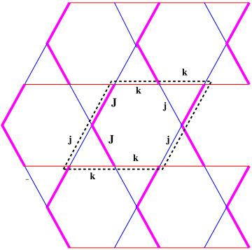
Figure 10: As Fig. 1 for a covering with one trimer per unit cell. In this case the paramagnetic unit cell contains a single trimer. The magnetic unit cell in the presence of antiferromagnetic trimer ordering is the same as that in Fig. 1 and contains two trimers.

$${\cal H} = \sum_{\bf R}\biggl{[}2k[n_{6}({\bf R})-n_{5}({\bf R})-3n_{4}({\bf R})-5n_{3}({\bf R})$$

$$-5n_{3}({\bf R}_{1})-3n_{4}({\bf R}_{1})-n_{5}({\bf R}_{1})+n_{6}({\bf R}_{1})]/9$$

$$+j[7n_{6}({\bf R})+5n_{5}({\bf R})+3n_{4}({\bf R})+n_{3}({\bf R})$$

$$+n_{3}({\bf R}_{1})+3n_{4}({\bf R}_{1})+5n_{5}({\bf R}_{1})+7n_{6}({\bf R}_{1})]/18$$

$$+\sum_{\mbox{\boldmath{$\delta$}}}j[-a_{4}^{\dagger}({\bf R})a_{4}({\bf R}+{\mbox{\boldmath{$\delta$}}})-a_{4}^{\dagger}({\bf R}+{\mbox{\boldmath{$\delta$}}})a_{4}({\bf R})$$

$$-3a_{6}^{\dagger}({\bf R})a_{6}({\bf R}+{\mbox{\boldmath{$\delta$}}})-3a_{6}^{\dagger}({\bf R}+{\mbox{\boldmath{$\delta$}}})a_{6}({\bf R})$$

$$-2a_{5}^{\dagger}({\bf R})a_{5}({\bf R}+{\mbox{\boldmath{$\delta$}}})-2a_{5}^{\dagger}({\bf R}+{\mbox{\boldmath{$\delta$}}})a_{5}({\bf R})]/18$$

$$+k[a_{4}^{\dagger}({\bf R})a_{4}({\bf R}+{\mbox{\boldmath{$\delta$}}})+a_{4}^{\dagger}({\bf R}+{\mbox{\boldmath{$\delta$}}})a_{4}({\bf R})$$

$$+2a_{5}^{\dagger}({\bf R})a_{5}({\bf R}+{\mbox{\boldmath{$\delta$}}})+2a_{5}^{\dagger}({\bf R}+{\mbox{\boldmath{$\delta$}}})a_{5}({\bf R})/36$$

$$+3a_{6}^{\dagger}({\bf R})a_{6}({\bf R}+{\mbox{\boldmath{$\delta$}}})+3a_{6}^{\dagger}({\bf R}+{\mbox{\boldmath{$\delta$}}})a_{6}({\bf R})]/36\biggr{]}\ .$$

Appendix E Another trimer covering

In Fig. 10 we show another covering of the Kagomé lattice with trimers. If the trimers are antiferromagnetically ordered, then the magnetic unit cell is the same as that of Fig. 1 and one can verify that the spectrum within the ground manifold is again given by Eqs. (8) and (10).

References

- (1) M. Weistein, Phys. Rev. D 61, 034505 (2000).
- (2) D. Grohol and D. G. Nocera, Chem. Mater, 19, 3061 (2007).
- (3) M. Kohno, O. A. Starykh, and L. Balents, Nat. Phys. 3, 790 (2007).
- (4) M. Ishii, H. Tanaka, M. Hori, H. Uekusa, Y. Ohashi, K. Tatani, Y. Narumi, and K. Kindo, J. Phys. Soc. Jpn, 69, 340 (2000).
- (5) A. Furrer and H. U. Güdel, J. Magn. Magn. Mater. 14, 256 (1979).
- (6) U. Falk, A. Furrer, N. Furrer, H. U. Gúdel, and J. K. Kjems, Phys. Rev. B 35, 4893 (1987).
- (7) Y. Qiu, C. Broholm, S. Ishiwata, M. Azuma, M. Takano, R. Bewley, and W. J. L. Buyers, Phys. Rev. B 71, 214439 (2005).
- (8) A. Podlesnyak, V. Pomjakushin, E. Pomjakushina, K. Conder, and A. Furrer, Phys. Rev. B 76, 064420 (2007).
- (9) K. Okamoto, T. Tonegawa, Y. Takahashi, and M. Kaburagi, J. Phys.: Condens. Matter 11, 10485 (1999).
- (10) A. Honecker and A. Läuchli, Phys. Rev. B 63, 174407 (2001).
- (11) S.-H. Lee, H. Kikuchi, Y. Qiu, B. Lake, Q. Huang, K. Habicht, and K. Keefer, Nature Mater. 6, 853 (2007).
- (12) J.-H. Kim, S. Ji, S.-H. Lee, B. Lake, T. Yildirim, H. Nojiri, H. Kikuchi, K. Habicht, Y. Qiu, and K. Kiefer, Phys. Rev. Lett. 101, 107201 (2008).
- (13) I. E. Dzialoshinskii, J. Phys. Chem. Solids 4, 241 (1958).
- (14) T. Moriya, Phys. Rev. 120, 91 (1960).
- (15) T. Yildirim and A. B. Harris, Phys. Rev. B 73, 214446 (2006).
- (16) O. Cépas, C. M. Fong, P. W. Leung, and C. Lhuillier, Phys. Rev. B 78 140405(R) (2008).
- (17) M. E. Rose, Elementary Theory of Angular Momentum (John Wiley & Sons, Inc. New York, 1957).
- (18) Note that if one uses the product wave functions of the Néel state, then the phase boundary between ferro- and antiferro-magnetic states occurs at . For large the zero-point corrections to the Néel state phase boundary are more severe than those to the trimer state phase boundary. The effects of such quantum fluctuations on phase boundaries were studied by E. Rastelli and A. B. Harris, Phys. Rev. B 41, 2449 (1990).
- (19) F. Keffer, in Encyclopedia of Physics: Ferromagnetism, edited by S. Flügge and H. P. J. Wijn (Springer, Berlin, Germany, 1966), p1.
- (20) V. Heine, Group Theory in Quantum Mechanics (Pergamon, New York, 1960) p284.
- (21) F. J. Dyson, Phys. Rev. 102, 1217 (1956); Phys. Rev. 102, 1230 (1956).
- (22) J. desCloizeaux and J. J. Pearson, Phys. Rev. 128, 2131 (1962).
- (23) T. Oguchi, Phys. Rev. 117, 117 (1959)
- (24) For a survey of the structural properties of polymorphs of Cu2(OH)2Cl see T. Malcherek and J. Schlüter, Acta. Cryst. B65, 334 (2009).
- (25) A. S. Wills and J.-Y. Henry, J. Phys.: Condens. Matter 20, 472206 (2008).