Capturing Patterns via Parsimonious $t$ Mixture Models

Abstract

This paper exploits a simplified version of the mixture of multivariate $t$-factor analyzers (MtFA) for robust mixture modelling and clustering of high-dimensional data that frequently contain a number of outliers. Two classes of eight parsimonious $t$ mixture models are introduced and computation of maximum likelihood estimates of parameters is achieved using the alternating expectation conditional maximization (AECM) algorithm. The usefulness of the methodology is illustrated through applications of image compression and compact facial representation.

Keywords:  Factor analysis; Facial representation; Image compression; PGMM; PTMM

1  Introduction

The mixture of factor analyzers (MFA) model, first introduced by Ghahramani and Hinton (1997) and further generalized by McLachlan and Peel (2000a), has provided a flexible dimensionality reduction approach to the statistical modelling of high-dimensional data arising from a wide variety of random phenomena. By combining the factor analysis model with finite mixture models, the MFA model allows simultaneous partitioning of the population into several subclasses while performing a local dimensionality reduction for each mixture component. In recent years, the study of MFA has received considerable interest; see McLachlan and Peel (2000b) and Fokoué and Titterington (2003) for some excellent reviews. McLachlan et al. (2002) and McLachlan et al. (2003) exploited the MFA approach to handle high-dimensional data such as clustering of microarray expression profiles. McNicholas and Murphy (2008) generalized the MFA model by introducing a family of parsimonious Gaussian mixture models (PGMMs).

In the MFA framework, component errors and factors are routinely assumed to have a Gaussian distribution due to their mathematical tractability and computational convenience. In practice, noise components or badly discrepant outliers often exist; the multivariate $t$ (MVT) distribution contains an additional tuning parameter, the degrees of freedom (df), which can be useful for outlier accommodation. Specifically, the density of a $g$-component multivariate $t$ mixture model is of the form

$$f(\mbox{\boldmath$y$})=\sum_{i=1}^{g}w_{i}t_{p}(\mbox{\boldmath$y$}|\mbox{\boldmath$\mu$}_{i},\mbox{\boldmath$\Sigma$}_{i},\nu_{i}),$$ (1)

where the $w_{i}$ are mixing proportions and $t_{p}(\mbox{\boldmath$y$}|\mbox{\boldmath$\mu$}_{i},\mbox{\boldmath$\Sigma$}_{i},\nu_{i})$ is the density of $p$-variate $t$ distribution with df $\nu_{i}$, mean vector $\mbox{\boldmath$\mu$}_{i}$, and scaling covariance matrix $\mbox{\boldmath$\Sigma$}_{i}$. Note that the general $t$ mixture (TMIX) model (1) has a total of $(g-1)+gp+gp(p+1)/2+g$ free parameters, of which $gp(p+1)/2+g$ parameters correspond to the component matrices $\mbox{\boldmath$\Sigma$}_{i}$ and df $\nu_{i}$, respectively. In a more parsimonious version of (1), wherein the $\mbox{\boldmath$\Sigma$}_{i}$ and $\nu_{i}$ are restricted to be identical across groups, the number of free parameters reduces to $(g-1)+gp+g(p+1)+p(p+1)/2$.

The TMIX model was first considered by McLachlan and Peel (1998) and Peel and McLachlan (2000), who presented expectation-maximization (EM) algorithms for parameter estimation and show the robustness of the model for clustering. Further developments along these directions followed, including work by Shoham (2002); Lin et al. (2004, 2009); Wang et al. (2004); Greselin and Ingrassia (2010); Andrews et al. (2011). An extension to mixture of $t$-factor analyzers (MtFA), adopting the family of MVT distributions for the component factor and errors, was first considered by McLachlan et al. (2007) and more recently by Andrews and McNicholas (2011a, b).

In this paper, our objective is to illustrate the efficacy of a class of TMIX models with several parsimonious covariance structures, called parsimonious $t$ mixture models (PTMMs). The PTMMs are based on assuming a constrained $t$-factor structure on each mixture component for parsimoniously modelling population heterogeneity in the presence of fat tails; the PTMMs are $t$-analogues of the PGMMs. We are devoted to developing additional tools for a simplified version of the MODt family of Andrews and McNicholas (2011b) and applying the proposed tools on image reconstruction tasks.

The EM algorithm (Dempster et al., 1977) and its extensions, such as the expectation conditional maximization (ECM) algorithm (Meng and Rubin, 1993) and the expectation conditional maximization either (ECME) algorithm (Liu and Rubin, 1994, 1995), have been practiced as useful tools for conducting maximum likelihood (ML) estimation in a variety of mixture modelling scenarios. To improve the computational efficiency for fitting PTMMs, we adopt a three-cycle AECM algorithm (Meng and van Dyk, 1997) that allows specification of different complete data at each cycle.

The rest of the paper is organized as follows. In Section 2, we briefly describe the single $t$ factor analysis model and study some related properties. In Section 3, we present the formulation of PTMM and discuss the methods for fitting these models. In Section 4, we demonstrate how PTMM can be applied to image compression and compact facial representation tasks. Some concluding remarks are given in Section 5.

2  The $t$ factor analysis model

We briefly review the $t$ factor analysis (tFA) model, which can be thought of as a single component MtFA model. Let $\mbox{\boldmath$Y$}=(\mbox{\boldmath$Y$}_{1},\ldots,\mbox{\boldmath$Y$}_{n})$ be a set of $p$-dimensional random vectors. In the tFA setting, each $\mbox{\boldmath$Y$}_{j}$ is modelled as

$$\mbox{\boldmath$Y$}_{j}=\mbox{\boldmath$\mu$}+\mbox{\bf B}\mbox{\boldmath$U$}_{j}+\mbox{\boldmath$\varepsilon$}_{j}$$ (2)

with

$$\left[\begin{array}[]{cc}\mbox{\boldmath$U$}_{j}\\ \mbox{\boldmath$\varepsilon$}_{j}\end{array}\right]\sim t_{q+p}\left(\left[\begin{array}[]{cc}\mbox{\bf 0}\\ \mbox{\bf 0}\\ \end{array}\right],\left[\begin{array}[]{cc}\mbox{\bf I}_{q}&\mbox{\bf 0}\\ \mbox{\bf 0}&\mbox{\boldmath$\Psi$}\\ \end{array}\right],\nu\right),$$

where $\mu$ is a $p$-dimensional mean vector, B is a $p\times q$ matrix of factor loadings, $\mbox{\boldmath$U$}_{j}$ is a $q$-dimensional ($q\ll p$) vector of latent variables called common factors, $\mbox{\boldmath$\varepsilon$}_{j}$ is $p$-dimensional vector of errors called specific factors, $\mbox{\bf I}_{q}$ is a $q$-dimensional identity matrix, $\mbox{\boldmath$\Psi$}={\rm diag}\{\psi_{1},\ldots,\psi_{p}\}$ is a diagonal matrix with positive entries, and $\nu$ is the df.

Note that $\mbox{\boldmath$U$}_{j}$ and $\mbox{\boldmath$\varepsilon$}_{j}$ are uncorrelated and marginally $t$-distributed, but not independent. Using the characterization of the $t$ distribution, model (2) can be hierarchically represented as

$$\mbox{\boldmath$Y$}_{j}\mid(\mbox{\boldmath$U$}_{j},\tau_{j}) \sim N_{p}(\mbox{\boldmath$\mu$}+\mbox{\bf B}\mbox{\boldmath$U$}_{j},\tau_{j}^{-1}\mbox{\boldmath$\Psi$}),$$

$$\mbox{\boldmath$U$}_{j}\mid\tau_{j} \sim N_{q}(\mbox{\bf 0},\tau^{-1}_{j}\mbox{\bf I}_{q}),$$

$$\tau_{j} \sim {\rm Gamma}(\nu/2,\nu/2),$$

where ${\rm Gamma}(\alpha,\beta)$ stands for the gamma distribution with mean $\alpha/\beta$. It follows that the marginal distribution of $\mbox{\boldmath$Y$}_{j}$, after integrating out $\mbox{\boldmath$U$}_{j}$ and $\tau_{j}$, can be expressed as $\mbox{\boldmath$Y$}_{j}\sim t_{p}(\mbox{\boldmath$\mu$},\mbox{\bf B}\mbox{\bf B}^{\rm T}+\mbox{\boldmath$\Psi$},\nu)$.

When handling high-dimensional data for large $p$ relative to $n$, say $p\gg n$, the inverse of $\mbox{\bf B}\mbox{\bf B}^{\rm T}+\mbox{\boldmath$\Psi$}$ plays an important role in computational complexity. In such a case, we use the following matrix inversion formula (Woodbury, 1950):

$$(\mbox{\bf B}\mbox{\bf B}^{\rm T}+\mbox{\boldmath$\Psi$})^{-1}=\mbox{\boldmath$\Psi$}^{-1}-\mbox{\boldmath$\Psi$}^{-1}\mbox{\bf B}(\mbox{\bf I}_{q}+\mbox{\bf B}^{\rm T}\mbox{\boldmath$\Psi$}^{-1}\mbox{\bf B})^{-1}\mbox{\bf B}^{\rm T}\mbox{\boldmath$\Psi$}^{-1},$$ (4)

which can be done more quickly because it involves only the low-dimensional $q\times q$ inverse plus the inversion of a diagonal $p\times p$ matrix. Moreover, the determinant of $\mbox{\bf B}\mbox{\bf B}^{\rm T}+\mbox{\boldmath$\Psi$}$ can be calculated as

$$|\mbox{\bf B}\mbox{\bf B}^{\rm T}+\mbox{\boldmath$\Psi$}|=|\mbox{\bf I}_{q}+\mbox{\bf B}^{\rm T}\mbox{\boldmath$\Psi$}^{-1}\mbox{\bf B}|\prod_{i=1}^{p}\psi_{i}.$$ (5)

The formulae (4) and (5) have been used many times before, including work by McLachlan and Peel (2000a) and McNicholas and Murphy (2008).

3  Parsimonious multivariate $t$ mixture models

Consider $n$ independent $p$-dimensional random vectors $\mbox{\boldmath$Y$}_{1},\ldots,\mbox{\boldmath$Y$}_{n}$ that come from a heterogeneous population with $g$ non-overlapping classes. Suppose that the density function of each feature $\mbox{\boldmath$Y$}_{j}$ can be modelled by a $g$-component MtFA:

$$f(\bm{Y}_{j}\mid\mbox{\boldmath$\Theta$})=\sum^{g}_{i=1}w_{i}t_{p}(\bm{Y}_{j}|\mbox{\boldmath$\mu$}_{i},\mbox{\bf B}_{i}\mbox{\bf B}^{\rm T}_{i}+\mbox{\boldmath$\Psi$}_{i},\nu_{i}),$$ (6)

where the $w_{i}$ are mixing proportions that are constrained to be positive and $\sum_{i=1}^{g}w_{i}=1$, $\mbox{\bf B}_{i}$ is a $p\times q$ matrix of factor loadings, and $\mbox{\boldmath$\Psi$}_{i}={\rm diag}\{\psi_{i1},\ldots,\psi_{ip}\}$ is a diagonal matrix. We use $\mbox{\boldmath$\Theta$}=(w_{1},\ldots,w_{g},\mbox{\boldmath$\theta$}_{1},\ldots,\bm{\theta}_{g})$ to represent all unknown parameters with $\mbox{\boldmath$\theta$}_{i}=(\mbox{\boldmath$\mu$}_{i},\mbox{\bf B}_{i},\bm{\Psi}_{i},\nu_{i})$ containing the parameters for the density of component $i$.

As in McLachlan et al. (2007), the MtFA model can be alternatively formulated by exploiting its link with the tFA model. Specifically, we assume that

$$\mbox{\boldmath$Y$}_{j}=\mbox{\boldmath$\mu$}_{i}+\mbox{\bf B}_{i}\mbox{\boldmath$U$}_{ij}+\mbox{\boldmath$\varepsilon$}_{ij}$$

with probability $w_{i}$, for $i=1,\ldots,g$ and $j=1,\ldots,n$, where $\mbox{\boldmath$U$}_{ij}$ and $\mbox{\boldmath$\varepsilon$}_{ij}$ are, respectively, the common and specific factors corresponding to component $i$. We assume that $\mbox{\boldmath$U$}_{ij}$ and $\mbox{\boldmath$\varepsilon$}_{ij}$ have a joint MVT distribution to be consistent with model (6) for the marginal distribution of $\mbox{\boldmath$Y$}_{j}$. Under a hierarchical mixture modelling framework, each $\mbox{\boldmath$Y$}_{j}$ is conceptualized to have originated from one of $g$ classes. It is convenient to construct unobserved allocation variables $\mbox{\boldmath$Z$}_{j}=(Z_{1j},\ldots,Z_{gj})^{\rm T}$, for $j=1,\ldots,n$, whose values are a set of binary variables with $Z_{ij}=1$ indexing so that $\mbox{\boldmath$Y$}_{j}$ belongs to class $i$ and are constrained to be $\sum_{i=1}^{g}Z_{ij}=1$ for each $j$. More specifically, $\mbox{\boldmath$Z$}_{j}$ is distributed as a multinomial random vector with one trial and cell probabilities $w_{1},\ldots,w_{g}$, denoted by $\mbox{\boldmath$Z$}_{j}\sim{\mathcal{M}}(1;w_{1},\ldots,w_{g})$. After a little algebra (cf. McLachlan et al., 2007), we have

$$\mbox{\boldmath$U$}_{ij}\mid(\mbox{\boldmath$Y$}_{j},Z_{ij}=1)\sim t_{q}\big{(}\mbox{\boldmath$\Gamma$}^{\rm T}_{i}(\mbox{\boldmath$Y$}_{j}-\mbox{\boldmath$\mu$}_{i}),\frac{\nu+\delta_{ij}}{\nu+p}\,\mbox{\boldmath$\Omega$}_{i},\nu+p\big{)},$$ (7)

where $\mbox{\boldmath$\Gamma$}_{i}=(\mbox{\bf B}_{i}\mbox{\bf B}^{\rm T}_{i}+\mbox{\boldmath$\Psi$}_{i})^{-1}\mbox{\bf B}_{i}$, $\mbox{\boldmath$\Omega$}_{i}=\mbox{\bf I}_{q}-\mbox{\boldmath$\Gamma$}^{\rm T}_{i}\mbox{\bf B}_{i}$ and $\delta_{ij}=(\mbox{\boldmath$Y$}_{j}-\mbox{\boldmath$\mu$}_{i})^{\rm T}(\mbox{\bf B}_{i}\mbox{\bf B}^{\rm T}_{i}+\mbox{\boldmath$\Psi$}_{i})^{-1}(\mbox{\boldmath$Y$}_{j}-\mbox{\boldmath$\mu$}_{i})$ denotes the Mahalanobis-squared distance between $\mbox{\boldmath$Y$}_{j}$ and $\mbox{\boldmath$\mu$}_{i}$.

Following McNicholas and Murphy (2008), we extend the MtFA model by allowing constraints across groups on matrices $\mbox{\bf B}_{i}$ and $\mbox{\boldmath$\Psi$}_{i}$. Specifically, we allow the following constraints on the scaling covariance matrices: $\mbox{\bf B}_{i}=\mbox{\bf B}$; $\mbox{\boldmath$\Psi$}_{i}=\mbox{\boldmath$\Psi$}$; or $\mbox{\boldmath$\Psi$}_{i}=\psi_{i}\mbox{\bf I}_{p}$, for $i=1,\ldots,g$. In addition, we consider the constraint $\nu_{i}=\nu~{}(i=1,\ldots,g)$ when we impose this constraint to reduce the number of parameter in PTMMs, our family of models (Table 1) is called ‘PTMM1’, and when the $\nu_{i}$ are allowed to vary across components, we call our family ‘PTMM2’. In this latter case (PTMM2), one simply adds $g-1$ parameters to the last column of Table 1. The number of free covariance parameters in the PTMM family — the union of PTMM1 and PTMM2 — can be reduced to as few as $qp-q(q-1)/2+2$ or inflated to as many as $g[pq-q(q-1)/2+p+1]$.

Table 1: The eight covariance structures, used by McNicholas and Murphy (2008), that form the basis of the PTMM considered herein. The “Constrained” in the columns “Loading”, “Error”, and “Isotropic” represent $\mbox{\bf B}_{i}=\mbox{\bf B}$, $\mbox{\boldmath$\Psi$}_{i}=\mbox{\boldmath$\Psi$}$ and $\psi_{ik}=\psi_{i}$ for $i=1,\ldots,g$ and $k=1,\ldots,k$, respectively.

Structure	Loading	Error	Isotropic	Number of parameters
CCC	Constrained	Constrained	Constrained	$(pq-q(q-1)/2)+1+1$
CCU	Constrained	Constrained	Unconstrained	$(pq-q(q-1)/2)+p+1$
CUC	Constrained	Unconstrained	Constrained	$(pq-q(q-1)/2)+g+1$
CUU	Constrained	Unconstrained	Unconstrained	$(pq-q(q-1)/2)+gp+1$
UCC	Unconstrained	Constrained	Constrained	$g(pq-q(q-1)/2)+1+1$
UCU	Unconstrained	Constrained	Unconstrained	$g(pq-q(q-1)/2)+p+1$
UUC	Unconstrained	Unconstrained	Constrained	$g(pq-q(q-1)/2)+g+1$
UUU	Unconstrained	Unconstrained	Unconstrained	$g(pq-q(q-1)/2)+gp+1$

The implementation of an efficient 3-cycle AECM algorithm for estimating PTMMs together with some practical issues including the specification of starting values, the stopping rule and the model selection criterion are described in Supplementary Material.

4  Applications

4.1   Image compression

A colour image is a digital image that includes 24-bit RGB colour information for each pixel. An RGB image is derived from the three primary colours — red (R), green (G), and blue (B) — for which each colour is 8 bits. The technique of image compression plays a central role in image transmission and storage for high quality. There are several unsupervised image compression approaches based on probabilistic models. The MFA model is well recognized as a dominant dimension reduction technique and is useful in block image transform coding (Ueda et al., 2000). In this subsection, we individually apply the PTMMs and PGMM to colour image compression and compare the quality of the reconstructed images. A $512\times 512$ RGB colour image ‘Lena’ (encoded in 24 bits per pixel) is subdivided into $n=16384$ non-overlapping RGB-blocks of $4\times 4\times 3$ pixels and each block is taken as a 48-dimensional data vector $y$. Let $\mathcal{Y}$ be a set of collected $y$ vector. Making a slight modification of Ueda et al. (2000), our compression procedure to transform the experimental image is summarized below.

1.

Set the desired number of components $g$ and dimensionality of factors $q$.

2.

Estimate $\Theta$ by fitting a parsimonious mixture model to $\mathcal{Y}$.

3.

Perform a model-based clustering according to the component membership of data point $y$, which is decided by maximizing the posterior probability $\Pr(Z_{ij}=1|\mbox{\boldmath$y$})$.

4.

For each $\mbox{\boldmath$y$}_{j}\in\mathcal{Y}$ classified to $\mathcal{C}_{i}$, calculate

$$\hat{\mbox{\boldmath$y$}}_{j}=\hat{\mbox{\boldmath$\mu$}}_{i}+\hat{\mbox{\bf B}}_{i}\hat{\mbox{\boldmath$U$}}_{ij},$$ (8)

where $\hat{\mbox{\boldmath$U$}}_{ij}=\hat{\mbox{\bf B}}^{\rm T}_{i}(\hat{\mbox{\bf B}}_{i}\hat{\mbox{\bf B}}^{\rm T}_{i}+\hat{\mbox{\boldmath$\Psi$}}_{i})^{-1}(\mbox{\boldmath$Y$}_{j}-\hat{\mbox{\boldmath$\mu$}}_{i})$ is the estimated posterior mean of (7).

5.

Reconstruct $\hat{\mbox{\boldmath$y$}}_{j}$, $j=1,\ldots,n$, into a compressed color image.

In what follows, we assumed that the characteristic of each components in the mixture model are the same, which leads to the MFA model with common factor loadings (CUU structure). The Lena image data are fitted by the CUU structure with $(g=4,q=4)$ and $(g=8,q=8)$ using the PGMM and PTMM approaches. To evaluate the quality of the reconstructed image, we compute the root mean squared error (RMSE) and peak signal-to-noise ratio (PSNR), which are widely used metrics in the image coding field. For an original color image $\{I_{R}(x,y),I_{G}(x,y),I_{B}(x,y)\}$ of size $M\times N$ and a reconstructed image $\{\hat{I}_{R}(x,y),\hat{I}_{G}(x,y),\hat{I}_{B}(x,y)\}$, the RMSE is defined as

$$\mbox{RMSE}=\sqrt{\frac{1}{3}\left(MSE_{R}+MSE_{G}+MSE_{B}\right)},$$

where

$$MSE_{R}=\frac{1}{MN}\sum_{x=1}^{M}\sum_{y=1}^{N}\big{[}I_{R}(x,y)-\hat{I}_{R}(x,y)\big{]}^{2},$$

and the other two quantities $MSE_{G}$ and $MSE_{B}$ are defined in the same fashion. The measure RMSE represents the average Euclidean distance from the original image to the output one. For a 24-bit colour $[0,255]^{3}$ image, the PSNR is given by

$$\mbox{PSNR}=20\log_{\rm 10}\left(\frac{255}{\mbox{RMSE}}\right).$$

Note that the higher PSNR value indicates a compressed (i.e., reconstructed) image of better quality.

Experimental results are provided in Table 2, including the log-likelihoods, the number of parameters, and BIC values, together with the RMSE and PSNR for the compressed images. The performance of PTMM1 and PTMM2 are almost the same in terms of RMSE and PSNR for the compressed images. Notably, the BIC and PSNR values obtained from the PTMM approaches are much higher than the PGMM for all cases.

Table 2: Comparisons of fitting adequacy and quality of image reconstruction using three CUU models with $(g=4;q=4)$ and $(g=8;q=8)$.

$(g=4;~{}q=4)$
Model	$\ell_{\mbox{max}}(\times 10^{3})$	$m$	BIC$(\times 10^{3})$	RMSE	PSNR
PGMM	2104.4	189	4206.8	7.62	30.5
PTMM1	2205.9	190	4409.7	5.22	33.8
PTMM2	2204.6	193	4407.1	5.26	33.7
$(g=8;~{}q=8)$
Model	$\ell_{\mbox{max}}(\times 10^{3})$	$m$	BIC$(\times 10^{3})$	RMSE	PSNR
PGMM	2235.1	363	4466.3	7.03	31.2
PTMM1	2348.8	364	4693.7	2.78	39.2
PTMM2	2351.2	371	4698.5	2.43	40.4

$\mbox{BIC}=2\ell_{\rm max}-m\log n$. Models with large BIC scores are preferred.

Figure 1 shows the original Lena image and three compressed images obtained by fitted the CUU $(g=8;q=8)$ models. The quality of the reconstructed images using the PTMMs is much better (i.e., smoother) than those reconstructed using the PGMM (for instance, observe the edge of Lena’s shoulder).

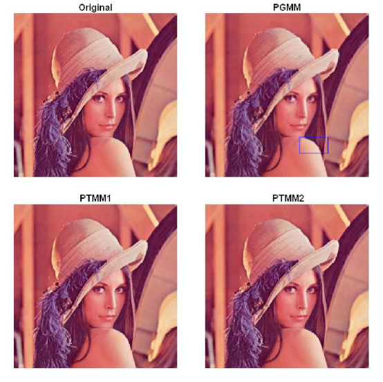
Figure 1: An example of Lena colour image reconstruction using three CUU models with $g=8$ and $q=8$.

4.2   Compact facial representation

Over the past few decades, numerous template matching approaches, along with their modifications and variants, have been proposed for human perception system face recognition; see Zhao et al. (2003) for an extensive survey. Motivated by a technique developed by Sirovitch and Kirby (1987), the eigenface method (Turk and Pentland, 1991) has become the most popular tool for facial feature extraction in computer vision research. Its implementation is primarily based on the use of PCA, also known as the Karhunen-Loève transform. The central idea of PCA is to find a multilinear subspace whose orthonormal basis maximizes the scatter matrix of all the projected samples.

Although the eigenface method is remarkably simple and quite straightforward, its performance depends heavily on pose, lighting and background conditions. Because PCA is a one-sample method, a single set of eigenfaces may not be enough to represent face images having a large amount of variation. Some efforts have been made to generalize it to the mixture-of-eigenfaces method Kim et al. (2002), which generates more than one set of eigenfaces for better representation of the whole face. However, such a method will produce an over-parameterized solution in many circumstances. To capture the heterogeneity among the underlying face images while maintaining parsimony in modeling, we apply the PTMM approach with common factor loadings (CUU) as a novel strategy for robust facial representation.

Consider a training set of $n$ face images ${I_{1},\ldots,I_{n}}$. Suppose that all images are exactly the same size; $a$ pixels in width by $b$ in height. Let $\mbox{\boldmath$y$}=\{\mbox{\boldmath$y$}_{j}={\rm vec}(I_{j})\}_{j=1}^{n}$ be the transformed image vectors taking intensity values in a $p$-dimensional image space, where $p=a\times b$. In what follows, we briefly review the eigenface method. Define the total scatter matrix of the sample images as

$$\mbox{\bf S}_{T}=\sum_{j=1}^{n}(\mbox{\boldmath$y$}_{j}-\bar{\mbox{\boldmath$y$}})(\mbox{\boldmath$y$}_{j}-\bar{\mbox{\boldmath$y$}})^{\rm T},$$

where $\bar{\mbox{\boldmath$y$}}$ is the mean image vector of all samples. In PCA, the optimal orthonormal basis vectors $\mbox{\boldmath$\Omega$}_{\rm PCA}\in R^{p\times K}$, where $K<<p$, are chosen to maximize the following objective function

$$\mbox{\boldmath$E$}_{\rm PCA}=[\mbox{\boldmath$e$}_{1}\cdots\mbox{\boldmath$e$}_{K}]=\mbox{argmax}_{\mbox{\boldmath$E$}}|\mbox{\boldmath$E$}^{\rm T}\mbox{\bf S}_{T}\mbox{\boldmath$E$}|,$$

where $\{\mbox{\boldmath$e$}_{k}\}_{k=1}^{K}$ is the set of $p$-dimensional vectors of $\mbox{\bf S}_{T}$ corresponding to the $K$ largest eigenvectors, which are referred to as eigenfaces in Turk and Pentland (1991) because they have exactly the same dimension as the original images. Each face image vector $\mbox{\boldmath$y$}_{i}$ can be represented as a linear combination of the best $K$ eigenvectors:

$$\hat{\mbox{\boldmath$y$}}^{{\rm PCA}}_{j}=\bar{\mbox{\boldmath$y$}}+\sum_{k=1}^{K}\omega_{jk}\mbox{\boldmath$e$}_{k},$$ (9)

where $\omega_{jk}=\mbox{\boldmath$e$}^{\rm T}_{k}(\mbox{\boldmath$y$}_{j}-\bar{\mbox{\boldmath$y$}})$.

As another illustration, we compare the face reconstruction performance among the PGMM and PTMM approaches using the image compression algorithm described in the above example and the eigenface method. We use the face images in the Yale face database, which contains 165 grayscale images of 15 individuals in GIF format. There are 11 images per person with pose and lighting variations, but for illustrative purposes and simplicity we consider only 11 images of one individual. For each image, we manually select the centers of eyes, denoted by $(x,y)$. The four boundaries of each cropped central part of the face are $x-60$, $x+60$, $y-100$, and $y+60$, which gives images of $121\times 161$ pixels as a sample in our experiment.

In this experiment, the 11 face images are trained by seven models: the PCA, PGMM, and PTMM1 models with CUU structure, where $K=q=5$ and $g=1,2,3$. The reconstructed images can be obtained by following two steps.

1.

In each model, the fitted vector is obtained as a reconstructed image, say $\hat{}\mbox{\boldmath$y$}_{j}$. For the PCA method, $\hat{}\mbox{\boldmath$y$}_{j}=\hat{}\mbox{\boldmath$y$}_{j}^{{\rm PCA}}$ as defined in (9). As for the PGMM and PTMM1, the solution is obtained by using (8).

2.

If the entries of $\hat{}\mbox{\boldmath$y$}_{j}$ do not fall in the color space, such as $[0,1]$, the reproductions $\hat{}\mbox{\boldmath$y$}_{j}^{\ast}$ are normalized by

$$\hat{y}_{jr}^{\ast}=\frac{\hat{y}_{jr}-\min\{\hat{}\mbox{\boldmath$y$}_{j}\}}{\max\{\hat{}\mbox{\boldmath$y$}_{j}\}-\min\{\hat{}\mbox{\boldmath$y$}_{j}\}},\quad\hbox{for $r=1,\ldots,p$}.$$

Figure 2 shows the original and the reconstructed images obtained from the seven training models. PCA clearly has the worst performance, while the PGMM and PTMM lead to somewhat comparable results. For explicitly measuring the reconstruction quality, we further calculated the RMSE, denoted by $[(\mbox{\boldmath$y$}_{j}-\hat{}\mbox{\boldmath$y$}_{j}^{\ast})^{\top}(\mbox{\boldmath$y$}_{j}-\hat{}\mbox{\boldmath$y$}_{j}^{\ast})]^{1/2}$, for each image and each model. Figure 3 displays the patterns of RMSE values. When comparing these models, smaller RMSEs indicate better reconstructions. In general, PTMM1 yields lower RMSE values than those from PGMM. As a result, we conclude that PTMM1 can be a prominent tool for facial coding.

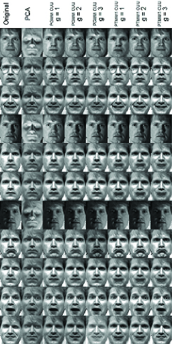
Figure 2: Reconstructed images based on PCA, PGMM and PTMM approaches. The first column shows sample images for one individual of the Yale database.

Figure 3: RMSE values of seven trained models for 11 face images.

5  Concluding remarks

We have utilized a class of parsimonious $t$ mixture models, called the PTMMs, which may create tremendous flexibility in robust clustering of high-dimensional data as they are relatively insensitive to outliers. This model-based tool allows practitioners to analyze heterogeneous multivariate data in a broad variety of considerations and works particularly well in high-dimensional settings. Numerical results show that the proposed PTMM approach performs reasonably well for the experimental image data. As pointed by by Zhao and Yu (2008) and Wang and Lin (2013), the convergence of the AECM algorithm can be painfully slow in certain situations. It is a worthwhile task to pursue some modified algorithms toward fast convergence.

Appendix

A: ML estimation via the AECM algorithm

We discuss how to carry out the AECM algorithm for computing the ML estimates of the parameters in PTMMs. To formulate the algorithm which consists of three cycles, we partition the unknown parameters $\Theta$ as $(\mbox{\boldmath$\Theta$}_{1},\mbox{\boldmath$\Theta$}_{2},\mbox{\boldmath$\Theta$}_{3})$, where $\mbox{\boldmath$\Theta$}_{1}$ contains $w_{i}$’s, $\mbox{\boldmath$\Theta$}_{2}$ contains $\mbox{\boldmath$\mu$}_{i}$’s and $\nu_{i}$’s, while $\mbox{\boldmath$\Theta$}_{3}$ contains $\mbox{\bf B}_{i}$’s and $\mbox{\boldmath$\Psi$}_{i}$’s. Let $\mbox{\boldmath$Z$}=(\mbox{\boldmath$Z$}_{1},\ldots,\mbox{\boldmath$Z$}_{n})$ be the collection of latent group labels. In the first cycle of the algorithm, we treat $Z$ as missing data. So the complete data is $\mbox{$\mbox{\boldmath$Y$}_{\hbox{aug}}^{[1]}$}=(\mbox{\boldmath$Y$},\mbox{\boldmath$Z$})$ and our aim is to estimate $\mbox{\boldmath$\Theta$}_{1}$ with $\mbox{\boldmath$\Theta$}_{2}$ and $\mbox{\boldmath$\Theta$}_{3}$ fixed at their current estimates $\hat{\mbox{\boldmath$\Theta$}}_{2}$ and $\hat{\mbox{\boldmath$\Theta$}}_{3}$.
       The log-likelihood of $\bm{\Theta}_{1}$ based on the complete data $\mbox{\boldmath$Y$}_{\hbox{aug}}^{[1]}$, apart from an additive constant, is given by

$$\ell_{c}^{[1]}(\mbox{\boldmath$\Theta$}_{1}|\mbox{$\mbox{\boldmath$Y$}_{\hbox{aug}}^{[1]}$}) = \sum_{j=1}^{n}\sum_{i=1}^{g}Z_{ij}\log w_{i}.$$ (10)

Conditioning on $Y$ and $\hat{\mbox{\boldmath$\Theta$}}$, taking expectation for (10) leads to

$$Q^{[1]}(\mbox{\boldmath$\Theta$}_{1}|\hat{\bm{\Theta}}) = \sum_{i=1}^{g}\sum_{j=1}^{n}\hat{z}_{ij}\log w_{i}$$ (11)

with

$$\hat{z}_{ij}=\frac{\hat{w}_{i}\,t_{p}(\bm{Y}_{j}\mid\hat{\mbox{\boldmath$\mu$}}_{i},\hat{\mbox{\bf B}}_{i}\hat{\mbox{\bf B}}^{\rm T}_{i}+\hat{\mbox{\boldmath$\Psi$}}_{i},\hat{\nu}_{i})}{\sum_{h=1}^{g}\hat{w}_{h}\,t_{p}(\bm{Y}_{j}\mid\hat{\mbox{\boldmath$\mu$}}_{h},\hat{\mbox{\bf B}}_{h}\hat{\mbox{\bf B}}^{\rm T}_{h}+\hat{\mbox{\boldmath$\Psi$}}_{h},\hat{\nu}_{h})}.$$

Maximizing (11) with respect to $w_{i}$, that restricted to $\sum_{i=1}^{g}w_{i}=1$, yields

$$\hat{w}_{i}=\frac{\sum_{j=1}^{n}\hat{z}_{ij}}{n}.$$

At the second cycle, when estimating $\mbox{\boldmath$\Theta$}_{2}$, we treat $\tau$ and $Z$ as the missing data. The log-likelihood function of $\mbox{\boldmath$\Theta$}_{2}$ based on the complete data $\mbox{$\mbox{\boldmath$Y$}_{\hbox{aug}}^{[2]}$}=(\mbox{$\mbox{\boldmath$Y$}_{\hbox{aug}}^{[1]}$},\mbox{\boldmath$\tau$})$ takes the form of

$$\ell_{c}^{[2]}(\mbox{\boldmath$\Theta$}_{2}|\mbox{$\mbox{\boldmath$Y$}_{\hbox{aug}}^{[2]}$}) = \sum_{j=1}^{n}\sum_{i=1}^{g}Z_{ij}\Big{\{}-\frac{1}{2}\tau_{j}(\bm{Y}_{j}-\mbox{\boldmath$\mu$}_{i})^{\rm T}(\hat{\mbox{\bf B}}_{i}\hat{\mbox{\bf B}}_{i}^{\rm T}+\hat{\mbox{\boldmath$\Psi$}}_{i})^{-1}(\bm{Y}_{j}-\mbox{\boldmath$\mu$}_{i})$$ (12)

$$+\frac{\nu_{i}}{2}\log\Big{(}\frac{\nu_{i}}{2}\Big{)}-\log\Gamma\Big{(}\frac{\nu_{i}}{2}\Big{)}+\frac{\nu_{i}}{2}(\log\tau_{j}-\tau_{j})\Big{\}}.$$

Conditioning on $Y$ and $\hat{\mbox{\boldmath$\Theta$}}$, taking expectation for (12) leads to

$$Q^{[2]}(\mbox{\boldmath$\Theta$}_{2}|\hat{\bm{\Theta}}) = -\frac{1}{2}\sum_{i=1}^{g}\sum_{j=1}^{n}\hat{z}_{ij}\hat{\tau}_{ij}(\mbox{\boldmath$Y$}_{j}-\mbox{\boldmath$\mu$}_{i})^{\rm T}(\hat{\mbox{\bf B}}_{i}\hat{\mbox{\bf B}}_{i}^{\rm T}+\hat{\mbox{\boldmath$\Psi$}}_{i})^{-1}(\bm{Y}_{j}-\mbox{\boldmath$\mu$}_{i})$$ (13)

$$+\sum_{i=1}^{g}\sum_{j=1}^{n}\hat{z}_{ij}\Big{[}\frac{\nu_{i}}{2}\log\Big{(}\frac{\nu_{i}}{2}\Big{)}-\log\Gamma\Big{(}\frac{\nu_{i}}{2}\Big{)}+\frac{\nu_{i}}{2}(\hat{\kappa}_{ij}-\hat{\tau}_{ij})\Big{]}$$

with

$$\hat{\tau}_{ij} = \frac{\hat{\nu}_{i}+p}{\hat{\nu}_{i}+\hat{\delta}_{ij}}~{}~{}\mbox{and}~{}~{}\hat{\kappa}_{ij}=\mbox{DG}\left(\frac{\hat{\nu}_{i}+p}{2}\right)-\log\left(\frac{\hat{\nu}_{i}+\hat{\delta}_{ij}}{2}\right),$$

where $\hat{\delta}_{ij}=(\mbox{\boldmath$Y$}_{j}-\hat{\mbox{\boldmath$\mu$}}_{i})^{\rm T}(\hat{\mbox{\bf B}_{i}}\hat{\mbox{\bf B}_{i}}^{\rm T}+\hat{\mbox{\boldmath$\Psi$}}_{i})^{-1}(\mbox{\boldmath$Y$}_{j}-\hat{\mbox{\boldmath$\mu$}}_{i})$ and DG$(\alpha)=\Gamma^{\prime}(\alpha)/\Gamma(\alpha)$ is the digamma function.
       Maximizing (13) with respect to $\mbox{\boldmath$\mu$}_{i}$ and $\nu_{i}$ yields

$$\hat{\mbox{\boldmath$\mu$}}_{i}=\frac{\sum_{j=1}^{n}\hat{z}_{ij}\hat{\tau}_{ij}\bm{Y}_{j}}{\sum_{j=1}^{n}\hat{z}_{ij}\hat{\tau}_{ij}},$$

and

$$\hat{\nu}_{i}={\rm argmax}_{\nu_{i}}\left\{\frac{\nu_{i}}{2}\log\Big{(}\frac{\nu_{i}}{2}\Big{)}-\log\Gamma\Big{(}\frac{\nu_{i}}{2}\Big{)}+\frac{\nu_{i}}{2}\left[\frac{\sum^{n}_{j=1}\hat{z}_{ij}(\hat{\kappa}_{ij}-\hat{\tau}_{ij})}{\sum^{n}_{j=1}\hat{z}_{ij}}\right]\right\},$$

which is equivalently the solution of the following equation:

$$\log\Big{(}\frac{\nu_{i}}{2}\Big{)}-{\rm DG}\Big{(}\frac{\nu_{i}}{2}\Big{)}+1+\frac{\sum^{n}_{j=1}\hat{z}_{ij}(\hat{\kappa}_{ij}-\hat{\tau}_{ij})}{\sum^{n}_{j=1}\hat{z}_{ij}}=0.$$

In the case of $\nu_{1}=\cdots=\nu_{g}=\nu$, we obtain $\hat{\nu}$ as the solution of the following equation:

$$\log\Big{(}\frac{\nu}{2}\Big{)}-{\rm DG}\Big{(}\frac{\nu}{2}\Big{)}+1+\frac{\sum^{g}_{i=1}\sum^{n}_{j=1}\hat{z}_{ij}(\hat{\kappa}_{ij}-\hat{\tau}_{ij})}{n}=0.$$

At the third cycle, when estimating $\mbox{\boldmath$\Theta$}_{3}$, we treat $U$, $\tau$ and $Z$ as the missing data. The log-likelihood function of $\mbox{\boldmath$\Theta$}_{3}$ based on the complete data $\mbox{$\mbox{\boldmath$Y$}_{\hbox{aug}}^{[3]}$}=(\mbox{$\mbox{\boldmath$Y$}_{\hbox{aug}}^{[2]}$},\mbox{\boldmath$U$})$ takes the form of

$$\ell_{c}^{[3]}(\mbox{\boldmath$\Theta$}_{3}\mid\mbox{$\mbox{\boldmath$Y$}_{\hbox{aug}}^{[3]}$}) = \sum_{i=1}^{g}\sum_{j=1}^{n}Z_{ij}\Big{\{}-\frac{1}{2}\log|\mbox{\boldmath$\Psi$}_{i}|-\frac{1}{2}\tau_{j}(\bm{Y}_{j}-\hat{\mbox{\boldmath$\mu$}}_{i})^{\rm T}\mbox{\boldmath$\Psi$}_{i}^{-1}(\bm{Y}_{j}-\hat{\mbox{\boldmath$\mu$}}_{i})$$ (14)

$$+\frac{1}{2}\tau_{j}(\bm{Y}_{j}-\hat{\mbox{\boldmath$\mu$}}_{i})^{\rm T}\mbox{\boldmath$\Psi$}_{i}^{-1}\mbox{\bf B}_{i}\mbox{\boldmath$U$}_{ij}+\frac{1}{2}\tau_{j}\mbox{\boldmath$U$}_{ij}^{\rm T}\mbox{\bf B}^{\rm T}_{i}\bm{\Psi}_{i}^{-1}(\bm{Y}_{j}-\hat{\mbox{\boldmath$\mu$}}_{i})$$

$$-\frac{1}{2}\tau_{j}\mbox{\boldmath$U$}_{ij}^{\rm T}\mbox{\bf B}^{\rm T}_{i}\bm{\Psi}_{i}^{-1}\mbox{\bf B}_{i}\mbox{\boldmath$U$}_{ij}\Big{\}}.$$

Therefore, the expectation of (14) conditioning on the observed data $Y$ and the updated vales of $\hat{\mbox{\boldmath$\Theta$}}$ is

$$Q^{[3]}(\mbox{\boldmath$\Theta$}_{3}\mid\hat{\bm{\Theta}}) = \frac{1}{2}\sum_{i=1}^{g}\hat{n}_{i}\log|\mbox{\boldmath$\Psi$}_{i}^{-1}|-\frac{1}{2}\sum_{i=1}^{g}\hat{n}_{i}\mbox{tr}\Big{\{}\mbox{\boldmath$\Psi$}_{i}^{-1}\mbox{\bf S}_{i}-\bm{\Psi}_{i}^{-1}\mbox{\bf B}_{i}\hat{\mbox{\boldmath$\Gamma$}}_{i}^{\rm T}\mbox{\bf S}_{i}$$

$$-\mbox{\boldmath$\Psi$}_{i}^{-1}\mbox{\bf S}_{i}\hat{\mbox{\boldmath$\Gamma$}}_{i}\mbox{\bf B}_{i}^{\rm T}+\mbox{\boldmath$\Psi$}_{i}^{-1}\mbox{\bf B}_{i}(\hat{\bm{\Omega}}_{i}+\hat{\mbox{\boldmath$\Gamma$}}_{i}\mbox{\bf S}_{i}\hat{\mbox{\boldmath$\Gamma$}}_{i}^{\rm T})\mbox{\bf B}_{i}^{\rm T}\Big{\}},$$

where $\hat{n}_{i}=\sum_{j=1}^{n}\hat{z}_{ij}$, $\mbox{\bf S}_{i}=\hat{n}^{-1}_{i}\sum_{j=1}^{n}\hat{z}_{ij}\hat{\tau}_{ij}(\bm{Y}_{j}-\hat{\mbox{\boldmath$\mu$}}_{i})(\bm{Y}_{j}-\hat{\mbox{\boldmath$\mu$}}_{i})^{\rm T}$ and $\hat{\bm{\Omega}}_{i}=\mbox{\bf I}_{q}-\hat{\bm{\Gamma}}^{\rm T}_{i}\hat{\mbox{\bf B}}_{i}$. The resulting CM-steps for the updates of $\mbox{\bf B}_{i}$ and $\mbox{\boldmath$\Psi$}_{i}$ under eight constrained/unconstrained situations are given in the next Section. Note that the above procedure is also applicable for the tFA model by treating $Z_{ij}=1$.

B: Calculations for eight parsimonious models

To facilitate the derivation, we adopt the following notation:

$$\tilde{\mbox{\bf S}}=\sum_{i=1}^{g}\hat{w}_{i}\mbox{\bf S}_{i}=n^{-1}\sum_{i=1}^{g}\sum_{j=1}^{n}\hat{z}_{ij}\hat{\tau}_{ij}(\bm{Y}_{j}-\hat{\mbox{\boldmath$\mu$}}_{i})(\bm{Y}_{j}-\hat{\mbox{\boldmath$\mu$}}_{i})^{\rm T}$$

B.1: Model CCC

For model CCC, we have $\mbox{\bf B}_{i}=\mbox{\bf B}$, $\bm{\Psi}_{i}=\bm{\Psi}=\psi\mbox{\bf I}_{p}$. The $Q^{[2]}$-function can be expressed as

$$Q^{[2]}=\frac{np}{2}p\log\psi^{-1}-\psi^{-1}\frac{n}{2}\Big{[}\mbox{tr}\{\tilde{\mbox{\bf S}}\}-2\mbox{tr}\{\mbox{\bf B}\hat{\bm{\Gamma}}^{\rm T}\tilde{\mbox{\bf S}}\}+\mbox{tr}\{\mbox{\bf B}(\hat{\mbox{\boldmath$\Omega$}}+\hat{\mbox{\boldmath$\Gamma$}}^{\rm T}\tilde{\mbox{\bf S}}\hat{\bm{\Gamma}})\mbox{\bf B}^{\rm T}\}\Big{]},$$

where $\hat{\mbox{\boldmath$\Gamma$}}=(\hat{\mbox{\bf B}}\hat{\mbox{\bf B}}^{\rm T}+\hat{\psi}\mbox{\bf I}_{p})^{-1}\hat{\mbox{\bf B}}$ and $\hat{\mbox{\boldmath$\Omega$}}=\mbox{\bf I}_{q}-\hat{\mbox{\bf B}}^{\rm T}\hat{\mbox{\boldmath$\Gamma$}}$. Differentiating $Q^{[2]}(\bm{\Theta}_{2}|\hat{\bm{\Theta}})$ with respect to B and $\psi^{-1}$, respectively, and set the derivations equal to zero, we obtain

$$\hat{\mbox{\bf B}}=\tilde{\mbox{\bf S}}\hat{\bm{\Gamma}}(\tilde{\bm{\Omega}}+\hat{\bm{\Gamma}}^{\rm T}\tilde{\mbox{\bf S}}\hat{\bm{\Gamma}})^{-1}~{}~{}\mbox{and}~{}~{}\hat{\psi}=\frac{1}{p}\mbox{tr}\{\tilde{\mbox{\bf S}}-\hat{\mbox{\bf B}}\hat{\mbox{\boldmath$\Gamma$}}^{\rm T}\tilde{\mbox{\bf S}}\}.$$

B.2: Model CCU

For model CCU, we have $\mbox{\bf B}_{i}=\mbox{\bf B}$, $\bm{\Psi}_{i}=\bm{\Psi}$. The $Q^{[2]}$-function can be expressed as

$$Q^{[2]}(\bm{\Theta}_{2}|\hat{\bm{\Theta}})=\frac{n}{2}\log|\bm{\Psi}^{-1}|-\frac{n}{2}\Big{[}\mbox{tr}\{\bm{\Psi}^{-1}\tilde{\mbox{\bf S}}\}-2\mbox{tr}\{\bm{\Psi}^{-1}\mbox{\bf B}\hat{\bm{\Gamma}}^{\rm T}\tilde{\mbox{\bf S}}\}+\mbox{tr}\{\bm{\Psi}^{-1}\mbox{\bf B}(\tilde{\bm{\Omega}}+\hat{\bm{\Gamma}}^{\rm T}\tilde{\mbox{\bf S}}\hat{\bm{\Gamma}})\mbox{\bf B}^{\rm T}\}\Big{]},$$

where $\hat{\mbox{\boldmath$\Gamma$}}=(\hat{\mbox{\bf B}}\hat{\mbox{\bf B}}^{\rm T}+\hat{\bm{\Psi}})^{-1}\hat{\mbox{\bf B}}$. Differentiating $Q^{[2]}(\bm{\Theta}_{2}|\hat{\bm{\Theta}})$ with respect to B and $\bm{\Psi}^{-1}$, respectively, and set the results equal to zero, we obtain

$$\hat{\mbox{\bf B}}=\tilde{\mbox{\bf S}}\hat{\bm{\Gamma}}(\tilde{\mbox{\boldmath$\Omega$}}+\hat{\mbox{\boldmath$\Gamma$}}^{\rm T}\tilde{\mbox{\bf S}}\hat{\mbox{\boldmath$\Gamma$}})^{-1}~{}~{}\mbox{and}~{}~{}\hat{\mbox{\boldmath$\Psi$}}=\mbox{Diag}\{\tilde{\mbox{\bf S}}-\hat{\mbox{\bf B}}\hat{\bm{\Gamma}}^{\rm T}\tilde{\mbox{\bf S}}\}.$$

B.3: Model CUC

For model CUC, we have $\mbox{\bf B}_{i}=\mbox{\bf B}$, $\bm{\Psi}_{i}=\psi_{i}\mbox{\bf I}_{p}$. The $Q^{[2]}$-function can be expressed as

$$Q^{[2]}=\sum^{g}_{i=1}\frac{\hat{n}_{i}}{2}\Big{[}p\log|\psi^{-1}_{i}|-\psi^{-1}_{i}\mbox{tr}\{\mbox{\bf S}_{i}\}+2\psi^{-1}_{i}\mbox{tr}\{\mbox{\bf B}\hat{\bm{\Gamma}}_{i}^{\rm T}\mbox{\bf S}_{i}\}-\psi^{-1}_{i}\mbox{tr}\{\mbox{\bf B}(\hat{\bm{\Omega}}_{i}+\hat{\bm{\Gamma}}_{i}^{\rm T}\mbox{\bf S}_{i}\hat{\bm{\Gamma}}_{i})\mbox{\bf B}^{\rm T}\}\Big{]},$$

where $\hat{\bm{\Gamma}}_{i}=(\hat{\mbox{\bf B}}\hat{\mbox{\bf B}}^{\rm T}+\hat{\psi}_{i}\mbox{\bf I}_{p})^{-1}\hat{\mbox{\bf B}}$ and $\hat{\bm{\Omega}}_{i}=\mbox{\bf I}_{q}-\hat{\bm{\Gamma}}_{i}^{\rm T}\hat{\mbox{\bf B}}$. Differentiating $Q^{[2]}(\bm{\Theta}_{2}|\hat{\bm{\Theta}})$ with respect to B and $\psi_{i}^{-1}$, respectively, and set the results equal to zero, we obtain

$$\hat{\mbox{\bf B}}=\left[\sum_{i=1}^{g}\frac{\hat{n}_{i}}{\psi_{i}}\mbox{\bf S}_{i}\hat{\bm{\Gamma}}_{i}\right]\left[\sum_{i=1}^{g}\frac{\hat{n}_{i}}{\psi_{i}}(\hat{\bm{\Omega}}_{i}+\hat{\bm{\Gamma}}_{i}^{\rm T}\mbox{\bf S}_{i}\hat{\bm{\Gamma}}_{i})\right]^{-1}$$

and

$$\hat{\psi}_{i}=\frac{1}{p}\mbox{tr}\{\mbox{\bf S}_{i}-2\hat{\mbox{\bf B}}\hat{\bm{\Gamma}}_{i}^{\rm T}\mbox{\bf S}_{i}+\hat{\mbox{\bf B}}(\hat{\bm{\Omega}}_{i}+\hat{\bm{\Gamma}}_{i}^{\rm T}\mbox{\bf S}_{i}\hat{\bm{\Gamma}}_{i})\hat{\mbox{\bf B}}^{\rm T}\}.$$

B.4: Model CUU

For model CUU we have $\mbox{\bf B}_{i}=\mbox{\bf B}$. The $Q^{[2]}$-function can be expressed as

$$Q^{[2]}=\sum^{g}_{i=1}\frac{\hat{n}_{i}}{2}\Big{[}\log|\mbox{\boldmath$\Psi$}^{-1}_{i}|-\mbox{tr}\{\mbox{\boldmath$\Psi$}^{-1}_{i}\mbox{\bf S}_{i}\}+2\mbox{tr}\{\mbox{\boldmath$\Psi$}^{-1}_{i}\bm{B}\hat{\bm{\Gamma}}_{i}^{\rm T}\mbox{\bf S}_{i}\}-\mbox{tr}\{\mbox{\boldmath$\Psi$}^{-1}_{i}\bm{B}(\hat{\bm{\Omega}}_{i}+\hat{\bm{\Gamma}}_{i}^{\rm T}\mbox{\bf S}_{i}\hat{\bm{\Gamma}}_{i})\bm{B}^{\rm T}\}\Big{]},$$

where $\hat{\bm{\Gamma}}_{i}=(\hat{\mbox{\bf B}}\hat{\mbox{\bf B}}^{\rm T}+\hat{\mbox{\boldmath$\Psi$}}_{i})^{-1}\hat{\mbox{\bf B}}$ and $\hat{\bm{\Omega}}_{i}=\mbox{\bf I}_{q}-\hat{\bm{\Gamma}}_{i}^{\rm T}\hat{\mbox{\bf B}}$. Differentiating $Q^{[2]}(\bm{\Theta}_{2}|\hat{\bm{\Theta}})$ with respect to B and $\mbox{\boldmath$\Psi$}_{i}^{-1}$, respectively, and set the results equal to zero, we have

$$\hat{\mbox{\boldmath$\Psi$}}_{i}=\mbox{diag}\{\mbox{\bf S}_{i}-2\hat{\mbox{\bf B}}\hat{\bm{\Gamma}}_{i}^{\rm T}\mbox{\bf S}_{i}+\hat{\mbox{\bf B}}(\hat{\bm{\Omega}}_{i}+\hat{\bm{\Gamma}}_{i}^{\rm T}\mbox{\bf S}_{i}\hat{\bm{\Gamma}}_{i})\hat{\mbox{\bf B}}^{\rm T}\}.$$

However, there is no closed form for the loading matrix $\hat{\mbox{\bf B}}$. One can solve it through a row-by-row manner. Set

$$\hat{\mbox{\bf B}}_{(p\times q)}=\left[\hat{\mbox{\boldmath$b$}}^{\rm T}_{1}\cdots\hat{\mbox{\boldmath$b$}}^{\rm T}_{k}\cdots\hat{\mbox{\boldmath$b$}}^{\rm T}_{p}\right]^{\rm T},$$

where $\hat{\mbox{\boldmath$b$}}_{k}=[\hat{b}_{k1}~{}\hat{b}_{k2}~{}\cdots~{}\hat{b}_{kq}]$ represents the $k$th row of the matrix $\hat{\mbox{\bf B}}$. Let $\mbox{\boldmath$R$}=\sum_{i=1}^{g}\hat{n}_{i}\mbox{\boldmath$\Psi$}_{i}^{-1}\mbox{\bf S}_{i}\hat{\bm{\Gamma}}_{i}$ and $\bm{r}_{h}$ be $h$th row of the matrix $R$. The $h$th row of $\hat{\mbox{\bf B}}$ can be expressed as

$$\hat{\bm{b}}_{h}\sum_{i=1}^{g}\frac{\hat{n}_{i}}{\hat{\psi}_{i(h)}}(\hat{\bm{\Omega}}_{i}+\hat{\bm{\Gamma}}_{i}^{\rm T}\mbox{\bf S}_{i}\hat{\bm{\Gamma}}_{i})=\bm{r}_{h},$$

where $\psi_{i(h)}$ denotes the $h$th element along the diagonal of $\mbox{\boldmath$\Psi$}_{i}$. Hence,

$$\hat{\bm{b}}_{h}=\bm{r}_{h}\left[\sum_{i=1}^{g}\frac{\hat{n}_{i}}{\hat{\psi}_{i(h)}}(\hat{\mbox{\boldmath$\Omega$}}_{i}+\hat{\mbox{\boldmath$\Gamma$}}_{i}^{\rm T}\mbox{\bf S}_{i}\hat{\mbox{\boldmath$\Gamma$}}_{i})\right]^{-1},~{}~{}\mbox{for}~{}h=1,\ldots,p.$$

B.5: Model UCC

For model UCC we have $\mbox{\boldmath$\Psi$}_{i}=\psi\mbox{\bf I}_{p}$. The $Q^{[2]}$-function can be expressed as

$$Q^{[2]}=\sum^{g}_{i=1}\frac{\hat{n}_{i}}{2}\Big{[}p\log|\psi^{-1}|-\psi^{-1}\mbox{tr}\{\mbox{\bf S}_{i}\}+2\psi^{-1}\mbox{tr}\{\mbox{\bf B}_{i}\hat{\bm{\Gamma}}_{i}^{\rm T}\mbox{\bf S}_{i}\}-\psi^{-1}\mbox{tr}\{\mbox{\bf B}_{i}(\hat{\bm{\Omega}}_{i}+\hat{\bm{\Gamma}}_{i}^{\rm T}\mbox{\bf S}_{i}\hat{\bm{\Gamma}}_{i})\mbox{\bf B}_{i}^{\rm T}\}\Big{]},$$

where $\hat{\mbox{\boldmath$\Gamma$}}_{i}=(\hat{\mbox{\bf B}_{i}}\hat{\mbox{\bf B}}_{i}^{\rm T}+\hat{\psi}\mbox{\bf I}_{p})^{-1}\hat{\mbox{\bf B}}_{i}$ and $\hat{\bm{\Omega}}_{i}=\bm{I}_{q}-\hat{\bm{\Gamma}}_{i}^{\rm T}\hat{\mbox{\bf B}}_{i}$. Differentiating $Q^{[2]}(\bm{\Theta}_{2}|\hat{\bm{\Theta}})$ with respect to $\mbox{\bf B}_{i}$ and $\psi^{-1}$, respectively, and set the results equal to zero, we obtain

$$\hat{\mbox{\bf B}}_{i}=\mbox{\bf S}_{i}\hat{\mbox{\boldmath$\Gamma$}}_{i}(\hat{\mbox{\boldmath$\Omega$}}_{i}+\hat{\mbox{\boldmath$\Gamma$}}_{i}^{\rm T}\mbox{\bf S}_{i}\hat{\mbox{\boldmath$\Gamma$}}_{i})^{-1}~{}~{}\mbox{and}~{}~{}\hat{\psi}=\frac{1}{p}\sum_{i=1}^{g}\hat{w}_{i}\mbox{tr}\{\mbox{\bf S}_{i}-\hat{\mbox{\bf B}}_{i}\hat{\bm{\Gamma}}_{i}^{\rm T}\mbox{\bf S}_{i}\}.$$

B.6: Model UCU

For model UCU we have $\mbox{\boldmath$\Psi$}_{i}=\mbox{\boldmath$\Psi$}$. The $Q^{[2]}$-function can be expressed as

$$Q^{[2]}=\sum^{g}_{i=1}\frac{\hat{n}_{i}}{2}\Big{[}\log|\mbox{\boldmath$\Psi$}^{-1}|-\mbox{tr}\{\mbox{\boldmath$\Psi$}^{-1}\mbox{\bf S}_{i}\}+2\mbox{tr}\{\mbox{\boldmath$\Psi$}^{-1}\mbox{\bf B}_{i}\hat{\bm{\Gamma}}_{i}^{\rm T}\mbox{\bf S}_{i}\}-\mbox{tr}\{\mbox{\boldmath$\Psi$}^{-1}\mbox{\bf B}_{i}(\hat{\mbox{\boldmath$\Omega$}}_{i}+\hat{\mbox{\boldmath$\Gamma$}}_{i}^{\rm T}\mbox{\bf S}_{i}\hat{\mbox{\boldmath$\Gamma$}}_{i})\mbox{\bf B}_{i}^{\rm T}\}\Big{]},$$

where $\hat{\mbox{\boldmath$\Gamma$}}_{i}=(\hat{\mbox{\bf B}_{i}}\hat{\mbox{\bf B}}_{i}^{\rm T}+\hat{\mbox{\boldmath$\Psi$}})^{-1}\hat{\mbox{\bf B}}_{i}$ and $\hat{\mbox{\boldmath$\Omega$}}_{i}=\mbox{\bf I}_{q}-\hat{\mbox{\boldmath$\Gamma$}}_{i}^{\rm T}\hat{\mbox{\bf B}}_{i}$. Differentiating $Q^{[2]}(\bm{\Theta}_{2}|\hat{\mbox{\boldmath$\Theta$}})$ with respect to $\mbox{\bf B}_{i}$ and $\mbox{\boldmath$\Psi$}^{-1}$, respectively, and set the results equal to zero, we obtain

$$\hat{\mbox{\bf B}}_{i}=\mbox{\bf S}_{i}\hat{\bm{\Gamma}}_{i}(\hat{\mbox{\boldmath$\Omega$}}_{i}+\hat{\bm{\Gamma}}_{i}^{\rm T}\mbox{\bf S}_{i}\hat{\mbox{\boldmath$\Gamma$}}_{i})^{-1}~{}~{}\mbox{and}~{}~{}\hat{\mbox{\boldmath$\Psi$}}=\sum_{i=1}^{g}\hat{w}_{i}\mbox{Diag}\{\mbox{\bf S}_{i}-\hat{\mbox{\bf B}}_{i}\hat{\mbox{\boldmath$\Gamma$}}_{i}^{\rm T}\mbox{\bf S}_{i}\}.$$

B.7: Model UUC

For model UUC we have $\mbox{\boldmath$\Psi$}_{i}=\psi_{i}\mbox{\bf I}_{p}$. The $Q^{[2]}$-function can be expressed as

$$Q^{[2]}=\sum^{g}_{i=1}\frac{\hat{n}_{i}}{2}\Big{[}p\log|\psi_{i}^{-1}|-\psi_{i}^{-1}\mbox{tr}\{\mbox{\bf S}_{i}\}+2\psi_{i}^{-1}\mbox{tr}\{\mbox{\bf B}_{i}\hat{\bm{\Gamma}}_{i}^{\rm T}\mbox{\bf S}_{i}\}-\psi_{i}^{-1}\mbox{tr}\{\mbox{\bf B}_{i}(\hat{\bm{\Omega}}_{i}+\hat{\bm{\Gamma}}_{i}^{\rm T}\mbox{\bf S}_{i}\hat{\bm{\Gamma}}_{i})\mbox{\bf B}_{i}^{\rm T}\}\Big{]},$$

where $\hat{\mbox{\boldmath$\Gamma$}}_{i}=(\hat{\mbox{\bf B}_{i}}\hat{\mbox{\bf B}}_{i}^{\rm T}+\hat{\psi}_{i}\mbox{\bf I}_{p})^{-1}\hat{\mbox{\bf B}}_{i}$ and $\hat{\mbox{\boldmath$\Omega$}}_{i}=\mbox{\bf I}_{q}-\hat{\mbox{\boldmath$\Gamma$}}_{i}^{\rm T}\hat{\mbox{\bf B}}_{i}$. Differentiating $Q^{[2]}(\bm{\Theta}_{2}|\hat{\bm{\Theta}})$ with respect to $\mbox{\bf B}_{i}$ and $\psi_{i}^{-1}$, respectively, and set the results equal to zero, we obtain

$$\hat{\mbox{\bf B}}_{i}=\mbox{\bf S}_{i}\hat{\bm{\Gamma}}_{i}(\hat{\mbox{\boldmath$\Omega$}}_{i}+\hat{\mbox{\boldmath$\Gamma$}}_{i}^{\rm T}\mbox{\bf S}_{i}\hat{\mbox{\boldmath$\Gamma$}}_{i})^{-1}~{}~{}\mbox{and}~{}~{}\hat{\psi}_{i}=\frac{1}{p}\mbox{ tr}\{\mbox{\bf S}_{i}-\hat{\mbox{\bf B}}_{i}\hat{\bm{\Gamma}}_{i}^{\rm T}\mbox{\bf S}_{i}\}.$$

B.8: Model UUU

For model UUU, there are no constraints, so that

$$Q^{[2]}=\sum_{i=1}^{g}\frac{\hat{n}_{i}}{2}\Big{[}\log|\bm{\Psi}_{i}^{-1}|-\mbox{tr}\{\bm{\Psi}_{i}^{-1}\mbox{\bf S}_{i}\}+2\mbox{tr}\{\bm{\Psi}_{i}^{-1}\mbox{\bf B}_{i}\hat{\bm{\Gamma}}_{i}^{\rm T}\mbox{\bf S}_{i}\}-\mbox{tr}\{\bm{\Psi}_{i}^{-1}\mbox{\bf B}_{i}(\hat{\bm{\Omega}}_{i}+\hat{\bm{\Gamma}}_{i}\mbox{\bf S}_{i}\hat{\bm{\Gamma}}_{i}^{\rm T})\mbox{\bf B}_{i}^{\rm T}\}\Big{]}.$$

Differentiating $Q^{[2]}(\bm{\Theta}_{2}|\hat{\bm{\Theta}})$ with respect to $\mbox{\bf B}_{i}$ and $\bm{\Psi}^{-1}_{i}$, respectively, and set the results equal to zero, we obtain

$$\hat{\mbox{\bf B}}_{i}=\mbox{\bf S}_{i}\hat{\mbox{\boldmath$\Gamma$}}_{i}(\hat{\bm{\Omega}}_{i}+\hat{\mbox{\boldmath$\Gamma$}}_{i}^{\rm T}\mbox{\bf S}_{i}\hat{\mbox{\boldmath$\Gamma$}}_{i})^{-1}~{}~{}\mbox{and}~{}~{}\hat{\bm{\Psi}}_{i}=\mbox{Diag}\{\mbox{\bf S}_{i}-\hat{\mbox{\bf B}}_{i}\hat{\mbox{\boldmath$\Gamma$}}_{i}^{\rm T}\mbox{\bf S}_{i}\}.$$

C: Some computational issues

C.1: Specification of initial values

We investigate the issue of getting admissible initial values for the implementation of the AECM algorithm. Essentially, good initial values of parameter estimates may speed up the convergence to the global maximum. A simple procedure of automatically constructing a set of initial values is outlined below.

1.

Perform the $k$-means algorithm initialized with a random seed. Subtract each observation from its initial cluster means. Then, do a single tFA fit to these “centering samples”. The resulting ML estimates $\hat{\mbox{\boldmath$\theta$}}=(\hat{\mbox{\bf B}},\hat{\mbox{\boldmath$\Psi$}},\hat{\psi},\hat{\nu})$ are taken as initial values of constrained parameters, namely $\hat{\mbox{\bf B}}^{(0)}=\hat{\mbox{\bf B}}$ for the common factor loading restriction, $\hat{\mbox{\boldmath$\Psi$}}^{(0)}=\hat{\mbox{\boldmath$\Psi$}}$ for the homoscedastic error covariance restriction, and $\hat{\psi}^{(0)}=\hat{\psi}$ for the isotropic restriction. The starting values for the dfs are set as $\hat{\nu}_{i}^{(0)}=50$, for $i=1,\ldots,g$, corresponding to an initial assumption of PGMM.

2.

Initialize the zero-one membership indicator $\hat{\mbox{\boldmath$Z$}}^{(0)}_{j}=\{\hat{z}^{(0)}_{ij}\}_{i=1}^{g}$ according to the $k$-means clustering result. The initial values for the mixing proportions and component locations are then given by

$$\hat{w}^{(0)}_{i}=\frac{\sum_{j=1}^{n}\hat{z}^{(0)}_{ij}}{n}~{}~{}\mbox{and}~{}~{}\hat{\mbox{\boldmath$\mu$}}^{(0)}_{i}=\frac{\sum_{j=1}^{n}\hat{z}^{(0)}_{ij}\mbox{\boldmath$y$}_{j}}{\sum_{j=1}^{n}\hat{z}^{(0)}_{ij}}.$$

3.

Divide the data into $g$ groups corresponding to $\hat{\mbox{\boldmath$Z$}}^{(0)}_{j}~{}(j=1,\ldots,n)$. Compute the sample variance-covariance matrix, namely $\mbox{\boldmath$V$}_{i}$, of each group. Following McNicholas and Murphy (2008), the initial values for the unconstrained $\mbox{\bf B}_{i}$ are set as

$$\hat{\mbox{\bf B}}^{(0)}_{i}=\Big{[}\sqrt{\hat{\lambda}_{i1}}\hat{\mbox{\boldmath$e$}}_{i1}~{}~{}\cdots~{}~{}\sqrt{\hat{\lambda}_{iq}}\hat{\mbox{\boldmath$e$}}_{iq}\Big{]},$$

where $\sqrt{\hat{\lambda}_{ir}}$ is the $r$th largest eigenvalue of $\mbox{\boldmath$V$}_{i}$ and $\hat{\mbox{\boldmath$e$}}_{ir}$ is the corresponding eigenvector. Straightforwardly, the initial values for $\mbox{\boldmath$\Psi$}_{i}$ and $\psi_{i}$ are respectively taken as

$$\ \begin{split}\hat{\mbox{\boldmath$\Psi$}}^{(0)}_{i}&={\rm diag}\{\mbox{\boldmath$V$}_{i}-\hat{\mbox{\bf B}}^{(0)}_{i}\hat{\mbox{\bf B}}^{(0){\rm T}}_{i}\},\\ \hat{\psi}^{(0)}_{i}&=\frac{1}{p}{\rm tr}\{\mbox{\boldmath$V$}_{i}-\hat{\mbox{\bf B}}^{(0)}_{i}\hat{\mbox{\bf B}}^{(0){\rm T}}_{i}\}.\end{split}$$

In practice, multiple modes typically exist on the complete-data log-likelihood surface. Thus, the algorithm needs to be initialized with a variety of starting values. This can be done by performing $k$-means clustering with various random seeds.

C.2: Stopping rule

To assess the convergence of the algorithm, various stopping criteria have been proposed in the literature. The most commonly used stopping criteria are based on lack-of-progress in the log-likelihood or parameter estimates and such criteria are not bona fide convergence criteria.
       We apply the Aitken acceleration scheme to determine the convergence of each AECM algorithm. The Aitken’s acceleration at iteration $k$ is defined by

$$a^{(k)}=\frac{l^{(k+1)}-l^{(k)}}{l^{(k)}-l^{(k-1)}},$$

where for brevity of notation $l^{(k)}$ means the log-likelihood value evaluated at $\hat{\mbox{\boldmath$\Theta$}}^{(k)}$. The asymptotic estimate of the log-likelihood at iteration $k+1$ is given by

$$l^{(k+1)}_{\infty}=l^{(k)}+\frac{1}{1-a^{(k)}}(l^{(k+1)}-l^{(k)}).$$

The algorithm is claimed to have reached convergence when $|l^{(k+1)}_{\infty}-l^{(k)}|<\epsilon$, where $\epsilon$ is the desired tolerance. Unless otherwise stated, $\epsilon=10^{-5}$ herein.

C.3: Model selection

The widely used Bayesian information criterion can be used to choose the best member of the PTMM family and the number of factors. Herein, the BIC is defined as

$$\mbox{BIC}=2\ell_{\rm max}-m\log n,$$

where $\ell_{\rm max}$ is the maximized log-likelihood and $m$ is the number of free parameters in the model. Accordingly, models with large BIC scores are preferred.

References

- Ghahramani and Hinton (1997) Z. Ghahramani and G. E. Hinton, “The EM algorithm for factor analyzers”, Tech. Rep. CRG-TR-96-1, University Of Toronto, Toronto, 1997.
- McLachlan and Peel (2000a) G. J. McLachlan and D. Peel, “Mixtures of factor analyzers”, in “Proceedings of the Seventh International Conference on Machine Learning”, pp. 599–606. Morgan Kaufmann, San Francisco, 2000a.
- McLachlan and Peel (2000b) G. J. McLachlan and D. Peel, “Finite mixture models”, John Wiley & Sons, New York, 2000b.
- Fokoué and Titterington (2003) E. Fokoué and D. M. Titterington, “Mixtures of factor analysers. Bayesian estimation and inference by stochastic simulation”, Machine Learning 50 (2003) 73–94.
- McLachlan et al. (2002) G. J. McLachlan, R. W. Bean, and D. Peel, “A mixture model-based approach to the clustering of microarray expression data”, Bioinformatics 18 (2002), no. 3, 412–422.
- McLachlan et al. (2003) G. J. McLachlan, D. Peel, and R. W. Bean, “Modelling high-dimensional data by mixtures of factor analyzers”, Comput. Statist. Data Anal. 41 (2003), no. 3–4, 379–388.
- McNicholas and Murphy (2008) P. D. McNicholas and T. B. Murphy, “Parsimonious Gaussian mixture models”, Stat. Comput. 18 (2008) 285–296.
- McLachlan and Peel (1998) G. J. McLachlan and D. Peel, “Robust cluster analysis via mixtures of multivariate -distributions”, in “Lecture Notes in Computer Science”, vol. 1451, pp. 658–666. Springer-Verlag, Berlin, 1998.
- Peel and McLachlan (2000) D. Peel and G. J. McLachlan, “Robust mixture modeling using the distribution”, Stat. Comput. 10 (2000) 339–348.
- Shoham (2002) S. Shoham, “Robust clustering by deterministic agglomeration EM of mixtures of multivariate -distributions”, Pattern Recogn. 35 (2002), no. 5, 1127–1142.
- Lin et al. (2004) T. I. Lin, J. C. Lee, and H. F. Ni, “Bayesian analysis of mixture modelling using the multivariate distribution”, Stat. Comput. 14 (2004) 119–130.
- Lin et al. (2009) T. I. Lin, H. J. Ho, and P. S. Shen, “Computationally efficient learning of multivariate mixture models with missing information”, Comp. Stat. 24 (2009) 375–392.
- Wang et al. (2004) H. X. Wang, Q. B. Zhang, B. Luo, and S. Wei, “Robust mixture modelling using multivariate distribution with missing information”, Pattern Recogn. Lett. 25 (2004) 701–710.
- Greselin and Ingrassia (2010) F. Greselin and S. Ingrassia, “Constrained monotone EM algorithms for mixtures of multivariate distributions”, Stat. Comput. 20 (2010) 9–22.
- Andrews et al. (2011) J. L. Andrews, P. D. McNicholas, and S. Subedi, “Model-based classification via mixtures of multivariate -distributions”, Comput. Statist. Data Anal. 55 (2011), no. 1, 520–529.
- McLachlan et al. (2007) G. J. McLachlan, R. W. Bean, and L. B.-T. Jones, “Extension of the mixture of factor analyzers model to incorporate the multivariate -distribution”, Comput. Statist. Data Anal. 51 (2007), no. 11, 5327–5338.
- Andrews and McNicholas (2011a) J. L. Andrews and P. D. McNicholas, “Extending mixtures of multivariate -factor analyzers”, Stat. Comput. 21 (2011)a, no. 3, 361–373.
- Andrews and McNicholas (2011b) J. L. Andrews and P. D. McNicholas, “Mixtures of modified -factor analyzers for model-based clustering, classification, and discriminant analysis”, J. Statist. Plann. Inf. 141 (2011)b, no. 4, 1479–1486.
- Dempster et al. (1977) A. P. Dempster, N. M. Laird, and D. B. Rubin, “Maximum likelihood from incomplete data via the EM algorithm”, J. Roy. Statist. Soc. B 39 (1977), no. 1, 1–38.
- Meng and Rubin (1993) X.-L. Meng and D. B. Rubin, “Maximum likelihood estimation via the ECM algorithm: a general framework”, Biometrika 80 (1993) 267–278.
- Liu and Rubin (1994) C. Liu and D. B. Rubin, “The ECME algorithm: a simple extension of EM and ECM with faster monotone convergence”, Biometrika 81 (1994) 633–648.
- Liu and Rubin (1995) C. Liu and D. B. Rubin, “ML estimation of the distribution using EM and its extensions, ECM and ECME”, Statistica Sinica 5 (1995) 19–39.
- Meng and van Dyk (1997) X.-L. Meng and D. van Dyk, “The EM algorithm — an old folk song sung to a fast new tune (with discussion)”, J. Roy. Statist. Soc. B 59 (1997) 511–567.
- Woodbury (1950) M. A. Woodbury, “Inverting modified matrices”, Princeton University, Princeton, New Jersey, 1950.
- Ueda et al. (2000) N. Ueda, R. Nakano, Z. Ghahramani, and G. E. Hinton, “SMEM algorithm for mixture models”, Neural Computation 12 (2000) 2109–2128.
- Zhao et al. (2003) W. Zhao, R. Chellappa, A. Rosenfeld, and P. J. Phillips, “Face recognition: A literature survey”, ACM Computing Surveys 35 (2003) 399–458.
- Sirovitch and Kirby (1987) L. Sirovitch and M. Kirby, “Low-dimensional procedure for the characterization of human faces”, J. Optical Soc. of Am. 2 (1987) 519–524.
- Turk and Pentland (1991) M. Turk and A. Pentland, “Eigenfaces for recognition”, J. Cognitive Neuroscience 3 (1991) 71–86.
- Kim et al. (2002) H. C. Kim, D. Lim, and S. Y. Bang, “Face recognition using the mixture-of-eigenfaces method”, Patt. Recog. Lett. 23 (2002) 1549–1558.
- Zhao and Yu (2008) J. H. Zhao and P. L. H. Yu, “Fast ML estimation for the mixture of factor analyzers via an ECM algorithm”, IEEE Trans. on Neu. Net. 19 (2008) 1956–1961.
- Wang and Lin (2013) W. L. Wang and T. I. Lin, “An efficient ecm algorithm for maximum likelihood estimation in mixtures of -factor analyzers”, Comput. Statist. DOI 10.1007/s00180-012-0327-z (2013).