Floquet generation of Majorana end modes and topological invariants

Abstract

We show how Majorana end modes can be generated in a one-dimensional system by varying some of the parameters in the Hamiltonian periodically in time. The specific model we consider is a chain containing spinless electrons with a nearest-neighbor hopping amplitude, a $p$-wave superconducting term and a chemical potential; this is equivalent to a spin-1/2 chain with anisotropic $XY$ couplings between nearest neighbors and a magnetic field applied in the $\hat{z}$ direction. We show that varying the chemical potential (or magnetic field) periodically in time can produce Majorana modes at the ends of a long chain. We discuss two kinds of periodic driving, periodic $\delta$-function kicks and a simple harmonic variation with time. We discuss some distinctive features of the end modes such as the inverse participation ratio of their wave functions and their Floquet eigenvalues which are always equal to $\pm 1$ for time-reversal symmetric systems. For the case of periodic $\delta$-function kicks, we use the effective Hamiltonian of a system with periodic boundary conditions to define two topological invariants. The first invariant is a well-known winding number while the second invariant has not appeared in the literature before. The second invariant is more powerful in that it always correctly predicts the numbers of end modes with Floquet eigenvalues equal to $+1$ and $-1$, while the first invariant does not. We find that the number of end modes can become very large as the driving frequency decreases. We show that periodic $\delta$-function kicks in the hopping and superconducting terms can also produce end modes. Finally, we study the effect of electron-phonon interactions (which are relevant at finite temperatures) and a random noise in the chemical potential on the Majorana modes.

I Introduction

Topological phases of quantum matter have been extensively studied for several years hasan ; qi ; fidkowski1 . Typically, these are phases which have only gapped states in the bulk (which therefore do not contribute at low temperatures to properties like transport) but have gapless states at the boundaries. (For three-, two- and one-dimensional systems, the boundaries are given by surfaces, edges and end points respectively). Further, the number of species of gapless boundary modes is given by a topological invariant whose nature depends on the spatial dimensionality of the system and the symmetries that it possesses, like spin rotation symmetry, particle-hole symmetry and time-reversal symmetry. The significance of a topological invariant is that it does not change if the system is perturbed (say, by impurities), as long as the bulk states remain gapped and the symmetry of the system is not changed by the perturbation. Examples of systems with topological phases include two- and three-dimensional topological insulators, quantum Hall systems, and wires with $p$-wave superconductivity.

Recently, there has been considerable interest in systems in which the Hamiltonian varies with time in a periodic way which gives rise to some topological features kita1 ; lind1 ; jiang ; gu ; kita2 ; lind2 ; trif ; russo ; basti1 ; liu ; tong ; cayssol ; rudner ; basti2 ; tomka ; gomez ; dora ; katan ; kundu ; basti3 ; schmidt ; reynoso ; wu . Some of these papers have discussed boundary modes and topological invariants kita1 ; lind1 ; jiang ; trif ; liu ; tong ; cayssol ; rudner ; kundu . Recently a photonic topological insulator has been demonstrated experimentally; a two-dimensional lattice of helical waveguides has been shown to exhibit topologically protected edge states recht . However, the existence of topological invariants and the relation between them and the number of Majorana modes at the boundary seems to be unclear, particularly if the driving frequency is small tong . Further, the Majorana boundary modes are of two types (corresponding to eigenvalues of the Floquet operator being $+1$ or $-1$, as discussed below); it would be interesting to know how the numbers of these two types of modes can be obtained from a topological invariant. The effect of time-reversal symmetry breaking on the boundary modes have also not been studied in detail. In this paper, we address all these questions for a one-dimensional model where both Majorana end modes and topological invariants can be numerically studied without great difficulty.

The plan of this paper is as follows. In Sec. II we introduce the system of interest and review some of its properties. Our system is a tight-binding model of spinless electrons with $p$-wave superconducting pairing and a chemical potential. By the Jordan-Wigner transformation lieb , this can be shown to be equivalent to a spin-1/2 $XY$ chain placed in a magnetic field pointing in the $\hat{z}$ direction. We discuss the energy spectrum and the three phases that this model has when the Hamiltonian is time-independent. In Sec. III, we review the topological invariants which one-dimensional models with and without time-reversal symmetry have when periodic boundary conditions are imposed. In Sec. IV, we discuss our numerical method of studying the Floquet evolution and the modes which appear at the ends of a system when the Hamiltonian varies with time in a periodic way. In Sec. V, we study what happens when one of the terms in the Hamiltonian (the chemical potential in the electron language or the magnetic field in the spin language) is given a periodic $\delta$-function kick stock . We study the ranges of parameters in which Majorana end modes appear at the ends of an open system and various properties of these modes such as their number and Floquet eigenvalues. We then use the Floquet operator for a system with periodic boundary conditions to define two topological invariants. The first invariant is a winding number which gives the total number of end modes. The second invariant appears to be new; we find that it correctly predicts the numbers of end modes with Floquet eigenvalues equal to $+1$ and $-1$ separately. We find that end modes can either appear or disappear as the driving frequency is varied, and our second topological invariant predicts where this occurs. For a special choice of parameters, we are able to find analytical expressions for the wave functions of the Majorana end modes and to confirm that the second topological invariant correctly gives the numbers of end modes with Floquet eigenvalues equal to $\pm 1$. The effect of time-reversal symmetry breaking on the end modes is studied; we find that that the end modes may survive but they are no longer of the Majorana type. In Sec. VI, we briefly study what happens if the hopping amplitude and superconducting term are given periodic $\delta$-function kicks. We show that the effect of this on the Majorana end modes is quite different from the case in which the chemical potential is given $\delta$-function kicks. In Sec. VII, we consider the case in which the chemical potential varies in time in a simple harmonic way, and we show that the wave function of the end modes can change significantly with time. In Sec. VIII, we study the effects of some aperiodic perturbations such as electron-phonon interactions and noise on the Majorana end modes. We summarize our main results and point out some directions for future work in Sec. IX.

II The Model

We consider a lattice model of spinless electrons with a nearest-neighbor hopping amplitude $\gamma$, a $p$-wave superconducting pairing $\Delta$ between neighboring sites, and a chemical potential $\mu$. For a finite and open chain with $N$ sites, the Hamiltonian takes the form

$$H = \sum_{n=1}^{N-1}[\gamma(f_{n}^{\dagger}f_{n+1}+f_{n+1}^{\dagger}f_{n})+\Delta(f_{n}f_{n+1}+f_{n+1}^{\dagger}f_{n}^{\dagger})]$$ (1)

$$-\sum_{n=1}^{N}\mu(2f_{n}^{\dagger}f_{n}-1),$$

where $\gamma$, $\Delta$ and $\mu$ are all real; we may assume that $\gamma>0$ without loss of generality. In this section we will assume that all these parameters are time-independent. The operators $f_{n}$ in Eq. (1) satisfy the usual anticommutation relations $\{f_{m},f_{n}\}=0$ and $\{f_{m},f_{n}^{\dagger}\}=\delta_{mn}$. (We will set both Planck’s constant $\hbar$ and the lattice spacing equal to 1 in this paper). We introduce the Majorana operators

$$a_{2n-1}=f_{n}+f_{n}^{\dagger}~{}~{}~{}~{}{\rm and}~{}~{}~{}~{}a_{2n}=i(f_{n}-f_{n}^{\dagger}),$$ (2)

for $n=1,2,\cdots,N$. We can check that these are Hermitian operators satisfying $\{a_{m},a_{n}\}=2\delta_{mn}$. In terms of these operators, Eq. (1) takes the form

$$H = i~{}\sum_{n=1}^{N-1}~{}[~{}J_{x}a_{2n}a_{2n+1}~{}-~{}J_{y}a_{2n-1}a_{2n+2}]$$

$$+~{}i~{}\sum_{n=1}^{N}~{}\mu a_{2n-1}a_{2n},$$

$$J_{x} = \frac{1}{2}(\gamma-\Delta)~{}~{}~{}~{}{\rm and}~{}~{}~{}~{}J_{y}=\frac{1}{2}(\gamma+\Delta).$$ (3)

Note that the Hamiltonian is invariant under the parity transformation $\cal P$ corresponding to a reflection of the system about its mid-point, i.e., $a_{2n}\to(-1)^{n}a_{2N+1-2n}$ and $a_{2n+1}\to a_{2N-2n}$.

We can map the above system to a spin-1/2 $XY$ chain placed in a magnetic field pointing in the $\hat{z}$ direction. We define the Jordan-Wigner transformation from $N$ spin-1/2’s to $2N$ Majorana operators lieb ,

$$a_{2n-1} = \left(\prod_{j=1}^{n-1}\sigma_{j}^{z}\right)~{}\sigma_{n}^{x},$$

$$a_{2n} = \left(\prod_{j=1}^{n-1}\sigma_{j}^{z}\right)~{}\sigma_{n}^{y},$$ (4)

where the $\sigma_{n}^{a}$ denote the Pauli matrices at site $n$, and $n=1,2,\cdots,N$. Eq. (3) can then be rewritten as

$$H~{}=~{}-\sum_{n=1}^{N-1}~{}[~{}J_{x}\sigma_{n}^{x}\sigma_{n+1}^{x}~{}+~{}J_{y}\sigma_{n}^{y}\sigma_{n+1}^{y}]~{}-\sum_{n=1}^{N}~{}\mu\sigma_{n}^{z}.$$ (5)

In all our numerical calculations, we will set $\gamma=-\Delta$; this implies that $J_{y}=0$ and $J_{x}=\gamma$, so that our system will be equivalent to an Ising model (with interaction $J_{x}$) in a transverse magnetic field $\mu$.

The system discussed above is time-reversal symmetric. The time-reversal transformation involves complex conjugating all objects, including $i\to-i$. With the usual convention for the Pauli matrices, Eq. (4) implies that

$$a_{2n}\to-~{}a_{2n}~{}~{}~{}~{}{\rm and}~{}~{}~{}~{}a_{2n+1}\to a_{2n+1}.$$ (6)

Hence Eq. (3) is time-reversal symmetric.

The energy spectrum of this system in the bulk can be found by considering a chain with periodic boundary conditions. We define the Fourier transform $f_{k}=\frac{1}{\sqrt{N}}~{}\sum_{n=1}^{N}f_{n}e^{ikn}$, where the momentum $k$ goes from $-\pi$ to $\pi$ in steps of $2\pi/N$. Then Eq. (1)) can be written in momentum space as

$$H = 2(\gamma-\mu)f_{0}^{\dagger}f_{0}~{}+~{}2(-\gamma-\mu)f_{\pi}^{\dagger}f_{\pi}$$ (10)

$$+~{}\sum_{0<k<\pi}~{}\left(\begin{array}[]{cc}f_{k}^{\dagger}&f_{-k}\end{array}\right)~{}h_{k}~{}\left(\begin{array}[]{c}f_{k}\\ f_{-k}^{\dagger}\end{array}\right),$$

$$h_{k} = 2(\gamma\cos k-\mu)~{}\tau^{z}~{}+~{}2\Delta\sin k~{}\tau^{y},$$ (11)

where the $\tau^{a}$ are Pauli matrices denoting pseudo-spin. The dispersion relation follows from Eq. (11) and is given by gott1 ; gott2

$$E_{k}~{}=~{}\sqrt{4(\gamma\cos k-\mu)^{2}~{}+~{}4\Delta^{2}\sin^{2}k}.$$ (12)

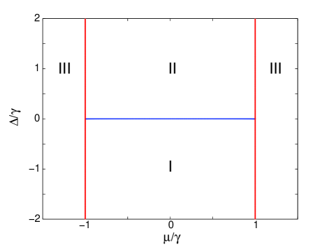
Figure 1: (Color online) Phase diagram of the model in Eq. (1) as a function of $\mu/\gamma$ and $\Delta/\gamma$. Phases I and II are topological while III is non-topological.

Depending on the values of $\gamma$, $\Delta$ and $\mu$, the system has three phases where $E_{k}$ is non-zero for all values of $k$ gott1 ; gott2 . The phase diagram is shown in Fig. 1. Phase I lies in the region $\Delta/\gamma<0$ and $-1<\mu/\gamma<1$. In this phase, a long and open chain has a zero energy Majorana mode at the left (right) end in which $a_{m}$ is non-zero only if $m$ is odd (even). This can be seen by considering the extreme case $J_{x}>0$ and $J_{y}=\mu=0$ in Eq. (3). Then that Hamiltonian is independent of $a_{1}$ at the left end and $a_{2N}$ at the right end; hence we have zero energy modes corresponding to these two operators. In the spin-1/2 language of Eq. (5), phase I corresponds to long-range ferromagnetic order of $\sigma^{x}$. Next, phase II lies in the region $\Delta/\gamma>0$ and $-1<\mu/\gamma<1$; here a long and open chain has a zero energy Majorana mode at the left (right) end in which $a_{m}$ is non-zero only if $m$ is even (odd). In the spin-1/2 language, this phase corresponds to long-range ferromagnetic order of $\sigma^{y}$. Finally, phase III consists of the two regions with $\mu/\gamma<-1$ and $\mu/\gamma>1$. In this phase, there are no zero energy Majorana modes at either end of an open chain. In the spin language, this is a paramagnetic phase with no long-range order. The three phases are separated from each other by quantum critical lines where the energy $E_{k}$ vanishes for some values of $k$. The critical lines are given by $\mu/\gamma=\pm 1$ for all values of $\Delta$, and $-1\leq\mu/\gamma\leq 1$ for $\Delta=0$. We will see in the next section that the three phases can be distinguished from each other by a topological invariant which is given by a winding number.

III Topological Invariants for a Time-independent Hamiltonian

In this section, we review the meaning of a topological phase and the topological invariants which exist for a one-dimensional system with a time-independent Hamiltonian which may or may not have time-reversal symmetry gott2 . This discussion will be useful for Sec. V where we will study if similar topological invariants exist for a system in which the Hamiltonian varies periodically with time.

We begin by considering a general Hamiltonian which is quadratic in terms of Majorana fermions,

$$H~{}=~{}i\sum_{m,n=1}^{2N}~{}a_{m}M_{mn}a_{n},$$ (13)

where $M$ is a real antisymmetric matrix; hence $iM$ is Hermitian. We can show that the non-zero eigenvalues of $iM$ come in pairs $\pm\lambda_{j}$ (where $\lambda_{j}>0$), and the corresponding eigenvectors are complex conjugates of each other, $x_{j}$ and $x^{*}_{j}$. This follows because $iMx_{j}=\lambda_{j}x_{j}$ implies $iMx_{j}^{*}=-\lambda_{j}x^{*}_{j}$. The zero eigenvalues must be even in number and their eigenvectors can be chosen to be real. This is because $iMx_{j}=0$ implies $iMx^{*}_{j}=0$, and we can then choose the eigenvectors to be the real combinations $x_{j}+x^{*}_{j}$ and $i(x_{j}-x^{*}_{j})$.

Given the time-reversal transformation in Eq. (6), we see that the Hamiltonian in Eq. (13) will have time-reversal symmetry if the matrix elements $M_{mn}$ are zero whenever both $m$ and $n$ are even or both are odd. Further, let us assume that the system is translation invariant and has periodic boundary conditions so that $M_{mn}$ is only a function of $m-n$ modulo $2N$. Defining the Dirac fermions $f_{n}$ using Eq. (2), we then find that the Hamiltonian will have the form given in Eq. (11), with gott2

$$h_{k}~{}=~{}a_{2,k}~{}\tau^{y}~{}+~{}a_{3,k}~{}\tau^{z},$$ (14)

where $a_{2/3,k}$ are some real and periodic functions of $k$. The corresponding dispersion is then given by $E_{k}=\sqrt{a_{2,k}^{2}+a_{3,k}^{2}}$. Although Eq. (11) defines $a_{2/3,k}$ only for $0\leq k\leq\pi$, it is convenient to analytically continue these definitions to the entire range $-\pi\leq k\leq\pi$. Next we map $h_{k}$ to the vector $\vec{V}_{k}=a_{2,k}\hat{y}+a_{3,k}\hat{z}$ in the $y-z$ plane. Let us define the angle $\phi_{k}=\tan^{-1}(a_{3,k}/a_{2,k})$ made by the vector $\vec{V}_{k}$ with respect to the $\hat{z}$ axis. Following Refs. [niu, ; tong, ], we now define a winding number by following the change in $\phi_{k}$ as we go around the Brillouin zone, i.e.,

$$W~{}=~{}\int_{-\pi}^{\pi}~{}\frac{dk}{2\pi}~{}\frac{d\phi_{k}}{dk}.$$ (15)

This can take any integer value and is a topological invariant, namely, it does not change under small changes in $h_{k}$ unless $h_{k}$ happens to pass through zero for some value of $k$ in which case the winding number becomes ill-defined; this can only happen if the energy $E_{k}=0$ at some value of $k$ which means that the bulk gap is zero. In a gapped phase, therefore, Eq. (15) defines a $Z$-valued topological invariant. We call a phase topological if $W\neq 0$; such a phase will have $W$ zero energy Majorana modes at each end of long chain gott2 . If $W=0$, the phase is non-topological and does not have any Majorana end modes.

We can now look at the three phases discussed after Eq. (12). We discover, by taking appropriate limits (like $\mu\ll\gamma,~{}\Delta$ or $\mu\gg\gamma,~{}\Delta$) that the winding number takes the values $-1$, $+1$ and $0$ in phases I, II and III respectively.

Next, we note that if time-reversal symmetry breaking terms were present in the Hamiltonian in (13), terms proportional to $\tau^{x}$ and the identity matrix $I$ will appear in $h_{k}$ in addition to terms proportional to $\tau^{y}$ and $\tau^{z}$. Then as $k$ goes from $-\pi$ to $\pi$, $h_{k}$ will generate a closed curve in three or four dimensions instead of only two dimensions, and it would not be possible to define a winding number as a topological invariant. However, it turns out that one can define a $Z_{2}$-valued topological invariant in that case kitaev ; gott2 . We find that at $k=0$ and $\pi$, $h_{k}$ only has a component along $\tau^{z}$; this is essentially because $k=-k$ in those two cases, hence terms proportional to $\tau^{x}$, $\tau^{y}$ and $I$ cannot appear in $h_{k}$. Let us denote $h_{0}=g_{0}\tau^{z}$ and $h_{\pi}=g_{\pi}\tau^{z}$. Assuming that we are in a gapped phase, so that $h_{k}\neq 0$ for all values of $k$, the $Z_{2}$-valued topological invariant is defined as $\nu=sgn(g_{0}g_{\pi})$ (here $sgn$ denotes the signum function). If $\nu=-1$, the phase is topological and has one zero energy Majorana mode at each end of a long chain, but if $\nu=1$, the phase is non-topological and does not have any Majorana end modes.

Finally, we can ask what would happen if one considered a time-reversal symmetric system which is in a topological phase with winding number $W$ (and hence has $W$ zero energy Majorana modes at each end of a long chain), and introduced a weak time-reversal breaking term in the Hamiltonian. Generally, what happens is that pairs of end modes move away from zero energy to energies $\pm E$; the number of modes which remain at zero energy (and hence are Majorana modes) is $1$ if $W$ is odd and zero if $W$ is even. Thus, the $Z$-valued invariant $W$ would reduce to the $Z_{2}$-valued invariant $\nu$ as $\nu=(-1)^{W}$.

IV Floquet Evolution

We will now study what happens when the Hamiltonian varies periodically in time, namely, the matrix $M$ in Eq. (13) changes with time as $M(t)$ such that $M(t+T)=M(t)$, where $T$ denotes the time period.

We consider the Heisenberg operators $a_{n}(t)$. These satisfy the equations

$$\frac{da_{n}(t)}{dt}~{}=~{}i~{}[H(t),a_{n}(t)].$$ (16)

Given that $H(t)=i\sum_{mn}a_{m}(t)M_{mn}(t)a_{n}(t)$, we obtain

$$\frac{da_{m}(t)}{dt}~{}=~{}4\sum_{n=1}^{2N}~{}M_{mn}(t)~{}a_{n}(t).$$ (17)

If $a$ denotes the column vector $(a_{1}a_{2},\cdots,a_{2N})^{T}$ and $M$ denotes the matrix $M_{mn}$, we can write the above equation as $da(t)/dt=4M(t)a(t)$. The solution of this is given by

$$a(t) = U(t,0)~{}a(0),$$

$${\rm where}~{}~{}U(t_{2},t_{1}) = {\cal T}e^{4\int_{t_{1}}^{t_{2}}dtM(t)},$$ (18)

and $\cal T$ denotes the time-ordering symbol. The time evolution operator $U(t_{1},t_{2})$ is a unitary (in fact, real and orthogonal) matrix which can be numerically computed given the form of $M(t)$. It satisfies the properties $U(t_{2},t_{1})=U^{-1}(t_{1},t_{2})$ and $U(t_{3},t_{1})=U(t_{3},t_{2})U(t_{2},t_{1})$.

If $M(t)$ varies with a time period $T$, we will call $U(T,0)$ the Floquet operator. The eigenvalues of $U(T,0)$ are given by phases, $e^{i\theta_{j}}$, and they come in complex conjugate pairs if $e^{i\theta_{j}}\neq 1$. This is because $U(T,0)\psi_{j}=e^{i\theta_{j}}\psi_{j}$ implies that $U(T,0)\psi_{j}^{*}=e^{-i\theta_{j}}\psi_{j}^{*}$. For eigenvalues $e^{i\theta_{j}}=\pm 1$ (these eigenvalues may, in principle, appear with no degeneracy), the eigenvectors can be chosen to be real; one can show this using an argument similar to the one given above for zero eigenvalues of the matrix $iM$.

In Secs. V and VII, we will consider two kinds of periodic driving of the chemical potential $\mu(t)$ with a time period $T$, namely, periodic $\delta$-function kicks stock and a simple harmonic variation with time. In Sec. VI, we will consider what happens if the hopping amplitude and superconducting term are given periodic $\delta$-function kicks. In each case, we will look for eigenvectors of $U(T,0)$ which are localized near the ends of the chain. Before discussing the specific results in the next three sections, let us describe our method of finding Majorana end modes and some of their general properties.

A convenient numerical method for finding eigenvectors of $U(T,0)$ which are localized at the ends is to look at the inverse participation ratio (IPR). We assume that the eigenvectors, denoted as $\psi_{j}$, are normalized so that $\sum_{m=1}^{2N}|\psi_{j}(m)|^{2}=1$ for each value of $j$; here $m=1,2,\cdots,2N$ labels the components of the eigenvector. We then define the IPR of an eigenvector as $I_{j}=\sum_{m=1}^{2N}|\psi_{j}(m)|^{4}$. If $\psi_{j}$ is extended equally over all sites so that $|\psi_{j}(m)|^{2}=1/(2N)$ for each $m$, then $I_{j}=1/(2N)$; this will approach zero as $N\to\infty$. But if $\psi_{j}$ is localized over a distance $\xi$ (which is of the order of the decay length of the eigenvector and remains constant as $N\to\infty$), then we will have $|\psi_{j}(m)|^{2}\sim 1/\xi$ in a region of length $\xi$ and $\sim 0$ elsewhere; then we have $I_{j}\sim 1/\xi$ which will remain finite as $N\to\infty$. If $N$ is sufficiently large, a plot of $I_{j}$ versus $j$ will be able to distinguish between states which are localized (over a length scale $\ll N$) and states which are extended. Once we find a state $j$ for which $I_{j}$ is significantly larger than $1/(2N)$ (which is the value of the IPR for a completely extended state), we look at a plot of the probabilities $|\psi_{j}(m)|^{2}$ versus $m$ to see whether it is indeed an end state. Finally, we check if the form of $|\psi_{j}(m)|^{2}$ and the value of IPR remain unchanged if $N$ is increased.

In all the periodic driving protocols discussed in Secs. V, VI and VII, we find, for certain ranges of the parameter values, that $U(T,0)$ has one or more pairs of eigenvectors with substantial values of the IPR. For each such pair, we find that the corresponding Floquet eigenvalues are complex conjugates of each other and they are both close to 1 (or $-1$); the two eigenvalues approach 1 (or $-1$) as we increase the system size $N$ keeping all the other parameters the same. Let us denote the corresponding eigenvectors by $\psi_{1}(m)$ and $\psi_{2}(m)$, where $m=1,2,\cdots,2N$. In the limit that $N\to\infty$ and the eigenvalues approach 1 (or $-1$), any linear combination of $\psi_{1}$ and $\psi_{2}$ will also be an eigenvector of $U(T,0)$ with the same eigenvalue. In that limit, suppose that we find that the probabilities of the two orthogonal linear combinations, given by $|(\psi_{1}(m)\pm\psi_{2}(m))|^{2}$, are peaked close to $m=1$ and $2N$, and that they decay as $m$ moves away from 1 or $2N$. We can then interpret these linear combinations as edge states produced by the time-dependent chemical potential. The deviation of the two Floquet eigenvalues from 1 (or $-1$) is a measure of the tunneling between the two edge states. The larger the tunneling, the greater is the deviation of the eigenvalues from $\pm 1$; this, in turn, implies that the two edge states decay less rapidly as we go away from the ends of the chain since a slower decay increases the tunneling between the two states.

The situation discussed in the previous paragraph is similar in some respects to the problem of a time-independent double well potential in one dimension which is reflection symmetric about one point, say, $x=0$. Then the eigenstates of the Hamiltonian are simultaneously eigenstates of the parity operator. The lowest energy states in the parity even and parity odd sectors differ in energy by an amount which depends on the tunneling amplitude between the two wells; the corresponding wave functions, denoted by $\psi_{+}$ and $\psi_{-}$, are symmetric and antisymmetric combinations of wave functions which are localized in the two wells separately. In the limit that the tunneling amplitude goes to zero, the two states become degenerate in energy; further, the linear combinations $\psi_{+}\pm\psi_{-}$ describe states which are localized in the two separate wells. In our Floquet problem, the two end states with opposite parity have complex conjugate eigenvalues of $U(T,0)$ given by $e^{\pm i\theta}$. In the limit that $N\to\infty$ and the tunneling between the two states goes to zero, the eigenvalues of $U(T,0)$ must become degenerate; this can only happen if $e^{\pm i\theta}$ approach either $+1$ or $-1$.

Finally, after finding the end modes, we check if their wave functions are real in the limit of large $N$. We call the end modes Majorana if they satisfy three properties: their Floquet eigenvalues must be equal to $\pm 1$, they must be separated by a finite gap from all the other eigenvalues, and their wave functions must be real.

V Periodic $\delta$-function Kicks in Chemical Potential

In this section, we consider the case where the chemical potential is given $\delta$-function kicks periodically in time. One reason for choosing to consider periodic kicks is that this is known to produce interesting effects in quantum systems such as dynamical localization stock . We will also see that this system is considerably easier to study both numerically and analytically than the case of a simple harmonic time-dependence which will be discussed in Sec. VII.

We begin by taking the chemical potential in Eq. (3) to be of the form

$$\mu(t)~{}=~{}c_{0}~{}+~{}c_{1}\sum_{n=-\infty}^{\infty}\delta(t-nT),$$ (19)

where $T=2\pi/\omega$ is the time period and $\omega$ is the driving frequency. Using Eq. (6), we note that this system has time-reversal symmetry: $H^{*}(-t)=H(t)$ for all values of $t$. (In general, we say that a system has time-reversal symmetry if we can find a time $t_{0}$ such that $H^{*}(t_{0}-t)=H(t)$ for all $t$, and does not have time-reversal symmetry if no such $t_{0}$ exists). As discussed below, we numerically compute the operator $U(T,0)$ for various values of the parameters $\gamma$, $\Delta$, $c_{0}$, $c_{1}$, $\omega$ and the system size $N$. We then find all the eigenvalues and eigenvectors of $U(T,0)$. Since the system is invariant under parity, $\cal P$, one can choose the eigenvectors of $U(T,0)$ to also be eigenvectors of $\cal P$.

The Floquet operator for a periodic $\delta$-function kick can be written as a product of two terms: an evolution with a constant chemical potential $c_{0}$ for time $T$ followed by an evolution with a chemical potential $c_{1}\delta(t-T)$. Namely,

$$U(T,0)~{}=~{}e^{4M_{1}}~{}e^{4M_{0}T},$$ (20)

where $M_{0/1}$ are $(2N)$-dimensional antisymmetric matrices whose non-zero matrix elements can be found using Eqs. (3) and (13):

$$(M_{0})_{2n+1,2n} = -~{}(M_{0})_{2n,2n+1}~{}=~{}-\frac{1}{4}(\gamma-\Delta),$$

$$(M_{0})_{2n-1,2n+2} = -~{}(M_{0})_{2n+2,2n-1}~{}=~{}-\frac{1}{4}(\gamma+\Delta),$$

$$(M_{0})_{2n-1,2n} = -~{}(M_{0})_{2n,2n-1}~{}=~{}\frac{c_{0}}{2},$$

$$(M_{1})_{2n-1,2n} = -~{}(M_{1})_{2n,2n-1}~{}=~{}\frac{c_{1}}{2},$$ (21)

for an appropriate range of values of $n$. However, in order to make the time-reversal symmetry more transparent, it turns out to be more convenient to use the symmetrized expression

$$U(T,0)~{}=~{}e^{2M_{1}}~{}e^{4M_{0}T}~{}e^{2M_{1}}.$$ (22)

It is easy to show that the Floquet operators in Eqs. (20) and (22) have the same eigenvalues, while their eigenvectors are related by a unitary transformation. We will see below that the symmetrized form in Eq. (22) leads to some simplifications when we derive an effective Hamiltonian and a topological invariant.

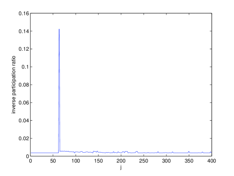
Figure 2: (Color online) IPRs of different eigenvectors of the Floquet operator for a 200-site system with a periodic $\delta$-function kick with $\gamma=1$, $\Delta=-1$, $c_{0}=2.5$, $c_{1}=0.2$ and $\omega=12$. The two eigenvectors with the largest IPRs both have an IPR equal to $0.142$ and Floquet eigenvalue equal to $-1$.

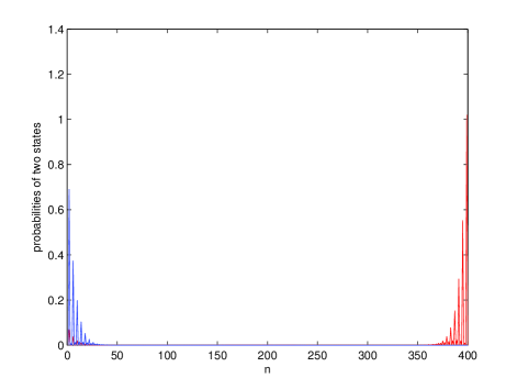
Figure 3: (Color online) Majorana end states for a 200-site system with a periodic $\delta$-function kick with $\gamma=1$, $\Delta=-1$, $c_{0}=2.5$, $c_{1}=0.2$ and $\omega=12$. These states correspond to the two eigenvectors with the largest IPRs in Fig. 2.

We now consider a 200-site system (hence with a $400$-dimensional Hamiltonian) with $\gamma=1$, $\Delta=-1$, $c_{0}=2.5$, $c_{1}=0.2$ and $\omega=12$. Fig. 2 shows the IPRs of the different eigenvectors. Two of the IPRs clearly stand out with a value of $0.142$ each. We find that they both have Floquet eigenvalue $e^{i\theta}=-1$, and the value of $\theta=\pi$ is separated by a gap of $0.148$ from the values of $\theta$ for all the other eigenvalues. The corresponding eigenvectors are localized at the two ends of the system and are real; the corresponding probabilities are shown in Fig. 3. The state at the left end has non-zero $a_{m}$ only if $m$ is even, while the state at the right end has non-zero $a_{m}$ only for $m$ odd. It is important to note that the periodic driving has produced Majorana end modes even though for the parameter values given above, $\mu(t)\geq\gamma$ at all values of $t$ according to Eq. (19), i.e., even though the corresponding time-independent system lies at all times in phase III (discussed in the paragraph after Eq. (12)) which is a non-topological phase.

We now vary $\omega$ to see how many Majorana end modes there are at each end of the system, and, more specifically, how many of these modes have Floquet eigenvalues equal to $\pm 1$. We denote the number of eigenvalues lying near $+1$ and $-1$ by the integers $N_{+}$ and $N_{-}$ respectively. Fig. 4 shows a plot of $N_{\pm}$ versus $\omega$ for a 200-site system with $\gamma=1$, $\Delta=-1$, $c_{0}=2.5$ and $c_{1}=0.2$. (We have checked that these eigenvalues are separated from all the other eigenvalues by a gap which remains finite as $N$ becomes large). We see that although the number of end modes is not a monotonic function of $\omega$, the number generally increases as $\omega$ decreases. The reason for this will become clear below.

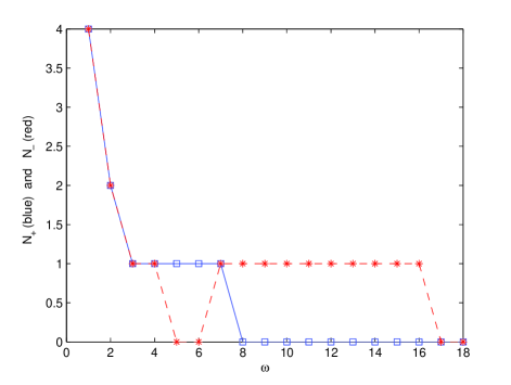
Figure 4: (Color online) Plot of the number of end states versus $\omega$ for a 200-site system, with Floquet eigenvalues $+1$ ($N_{+}$, blue squares) and $-1$ ($N_{-}$, red stars), for a periodic $\delta$-function kick with $\gamma=1$, $\Delta=-1$, $c_{0}=2.5$ and $c_{1}=0.2$.

V.1 Topological Invariants

We saw above that there are a number of Majorana end modes, which can be further separated into $N_{\pm}$ depending on whether the Floquet eigenvalues $e^{i\theta}$ lie near $+1$ or $-1$. Further, the eigenvalues $\theta=0$ and $\pi$ are separated from all the other eigenvalues by a gap which remains finite as $N\to\infty$. We then expect the integers $N_{+}$ and $N_{-}$ to be topological invariants, i.e., they will not change under small changes in the various parameters of the system. The only way in which these integers can change is if the eigenvalue gap closes and reopens as we vary the system parameters.

We therefore look for a topological invariant for this time-dependent problem kita1 ; jiang ; trif ; tong ; rudner . Interestingly, we will discover that we can define a topological invariant in two different ways: one is a winding number which only gives the total number of Majorana modes at each end of a chain, while the other also gives the individual values of $N_{+}$ and $N_{-}$ which are the numbers of end modes with Floquet eigenvalues equal to $+1$ and $-1$.

To define the topological invariants, we consider a system with periodic boundary conditions. Then the system is translation invariant and the momentum $k$ is a good quantum number; the system decomposes into a sum of subsystems labeled by different values of $k$ lying in the range $[0,\pi]$. For each value of $k$, we define a Floquet operator $U_{k}(T,0)$ which is a $2\times 2$ unitary matrix. Using Eqs. (11), (19) and (22), we find that

$$U_{k}(T,0)=e^{ic_{1}\tau^{z}}e^{-i2T[(\gamma\cos k-c_{0})\tau^{z}+\Delta\sin k\tau^{y}]}e^{ic_{1}\tau^{z}},$$ (23)

where we take $k$ to lie in the full range $-\pi\leq k\leq\pi$.

Let us assume that $2c_{1}/\pi$ is not equal to an integer and $\Delta\neq 0$. We now prove an interesting fact about $U_{k}(T,0)$, namely, that it can be equal to $\pm I$ only if $k=0$ or $\pi$ and if $T$ is given by a discrete set of values. First, given the above conditions on $c_{1}$ and $\Delta$, we can show that $U_{k}(T,0)\neq\pm I$ for any value of $k\neq 0$ or $\pi$. Next, if $k=0$ or $\pi$, we see from Eq. (23) that $U_{k}(T,0)\neq\pm I$ unless $2T(c_{0}\pm\gamma)+2c_{1}=n\pi$, i.e., unless $\omega=2\pi/T$ satisfies

$$\omega~{}=~{}\frac{4\pi(c_{0}\pm\gamma)}{n\pi-2c_{1}}$$ (24)

for some integer value of $n$. The $\pm$ sign in Eq. (24) corresponds to $k=\pi$ and $0$ respectively. Eq. (24) holds only for a discrete set of values $\omega$. For all other values of $\omega$, therefore, $U_{k}(T,0)$ will not be equal to $\pm I$ for any value of $k$. This also means that for all $k$, the Floquet eigenvalues (which are given by the eigenvalues of $U_{k}(T,0)$) will be separated by a gap from $\pm 1$. We are now ready to define our topological invariants.

First topological invariant: Given Eq. (23), let us define an effective Hamiltonian $h_{eff,k}$ as

$$U_{k}(T,0)~{}=~{}e^{-ih_{eff,k}}.$$ (25)

The structure of Eq. (23) is such that $h_{eff,k}$ takes the form

$$h_{eff,k}~{}=~{}a_{2,k}~{}\tau^{y}~{}+~{}a_{3,k}~{}\tau^{z}$$ (26)

as in Eq. (14). (Indeed, this is the reason we choose the Floquet operator of the form given in Eq. (22) rather than in Eq. (20)). Note that Eqs. (23) and (25) do not determine $h_{eff,k}$ uniquely. To define $h_{eff,k}$ uniquely, we impose the condition that the coefficients in Eq. (26) satisfy $0<\sqrt{a_{2,k}^{2}+a_{3,k}^{2}}<\pi$. (It is possible to impose this if $U_{k}(T,0)\neq\pm I$; this will be true if $\omega$ does not satisfy Eq. (24)). Given the form in Eq. (26), we can then compute a winding number $W$ as described in Eq. (15).

We note in passing that the condition $0<a_{2,k}^{2}+a_{3,k}^{2}<\pi$ implies that $h_{eff,k}$ can be mapped to a point on the surface of a sphere whose polar angles $(\alpha,\beta)$ are given by $\alpha=\sqrt{a_{2,k}^{2}+a_{3,k}^{2}}$ and $\beta=\tan^{-1}(a_{3,k}/a_{2,k})$. As $k$ goes from 0 to $2\pi$, we obtain a closed curve which does not pass through the north and south poles. The integer $W$ can then be related to the winding number of this curve around either the north pole or the south pole. Note that the winding numbers around the north and south pole are given by the same integer.

In Fig. 5, we show the closed curves in the $(a_{2,k},a_{3,k})$ plane for four values of $\omega$ for a 200-site system with $\gamma=1$, $\Delta=-1$, $c_{0}=2.5$ and a periodic $\delta$-function kick with $c_{1}=0.2$. For $\omega=3,~{}7,~{}12$ and 17, the winding numbers around the origin are given by 2, 2, 1 and 0 respectively. These agree exactly with the number of Majorana modes at each end of an open chain for those values of $\omega$ as shown in Fig. 6.

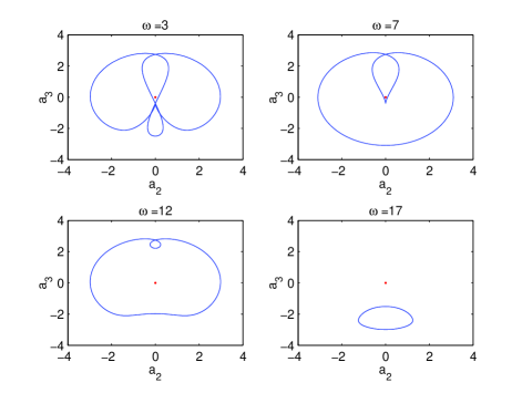
Figure 5: (Color online) Closed curves in the $(a_{2,k},a_{3,k})$ plane for $\omega=3,~{}7,~{}12$ and 17, for a 200-site system with $\gamma=1$, $\Delta=-1$, $c_{0}=2.5$ and a periodic $\delta$-function kick with $c_{1}=0.2$. The corresponding winding numbers around the origin (the point $(0,0)$ shown by a red dot) are given by 2, 2, 1 and 0 respectively.

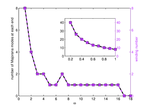
Figure 6: (Color online) Comparison of the number of Majorana modes at each end of a 200-site system (black solid, $y$-axis on left) and the winding number (magenta dashed, $y$-axis on right) as a function of $\omega$ from 1 to 18, for $\gamma=1$, $\Delta=-1$, $c_{0}=2.5$ and a periodic $\delta$-function kick with $c_{1}=0.2$. The inset shows a range of $\omega$ from $0.2$ to 1 where there is a large number of Majorana modes.

In Fig. 6, we compare the number of Majorana modes at each end of a chain and the winding number as a function of $\omega$, for a 200-site system with $\gamma=1$, $\Delta=-1$, $c_{0}=2.5$ and $c_{1}=0.2$. In preparing that figure, we have considered only those values of $\omega$ for which Eq. (24) is not satisfied. We see that the number of end modes and the winding number completely agree in the range $0.2\leq\omega\leq 18$. Note that in the limit $\omega\to\infty$, i.e., $T\to 0$, Eq. (23) becomes independent of $k$, and we therefore obtain a single point in the $(a_{2,k},a_{3,k})$ plane. This corresponds to a curve with zero winding number which is consistent with the observation that there is a maximum value of $\omega$ beyond which there are no Majorana end modes.

In Fig. 6, we have not shown the number of Majorana end modes for $\omega<0.2$. For small $\omega$, we see that the number of end modes increases. (We will make this more precise below). However, it becomes more and more difficult to identify the end modes as $\omega$ becomes small; we find that there are a large number of what appear to be end modes, but many of them have decay lengths which are not much smaller than the system sizes that we have considered and their Floquet eigenvalues differ slightly from $\pm 1$. Thus we have to go to very large system sizes to confirm if all of these are really Majorana end modes, i.e., if their Floquet eigenvalues approach $\pm 1$ and if these are separated from all other eigenvalues by a finite gap in the limit of infinite system size.

Second topological invariant: We observe that the momenta $k=0$ and $\pi$ play a special role since $U_{k}(T,0)$ can be equal to $\pm I$ at only those two values. Eq. (23) shows that $U_{0}(T,0)=e^{i\pi b_{0}\tau^{z}}$ and $U_{\pi}(T,0)=e^{i\pi b_{\pi}\tau^{z}}$, where we choose $b_{0/\pi}$ in the simplest possible way, namely,

$$b_{0} = \frac{4(c_{0}-\gamma)}{\omega}~{}+~{}\frac{2c_{1}}{\pi},$$

$$b_{\pi} = \frac{4(c_{0}+\gamma)}{\omega}~{}+~{}\frac{2c_{1}}{\pi},$$ (27)

where $\omega=2\pi/T$. We now define a finite line segment, called $L_{\omega}$, which goes from $b_{0}$ to $b_{\pi}$ in one dimension which we will call the $z$-axis.

For $\omega\to\infty$, the line $L_{\omega}$ collapses to a single point given by $z=2c_{1}/\pi$. We have assumed earlier that this is not an integer. As $\omega$ is decreased, $L_{\omega}$ will move and also increase in size. For our system parameters $\gamma=1$, $c_{0}=2.5$ and $c_{1}=0.2$, we find that the right end of $L_{\omega}$, given by $b_{\pi}$ in Eq. (27), crosses the point $z=n$ with $n=1$ at some value of $\omega$. At this point, we see from Eq. (23) that the Floquet eigenvalue at $k=\pi$ is equal to $e^{in\pi}=-1$. We therefore expect that when $\omega$ decreases a little more and $L_{\omega}$ includes the point $z=1$, a Majorana mode will appear at each end of an open chain with the Floquet eigenvalue equal to $-1$. For our parameters, we therefore predict, by setting $b_{\pi}=1$, that the first Majorana end mode will appear at $\omega\simeq 16.04$. This agrees well with Fig. 6 which shows that a Majorana end mode first appears in the range $16\leq\omega\leq 17$ and it has a Floquet eigenvalue equal to $-1$. As $\omega$ is decreased further, the right end of $L_{\omega}$ given by $b_{\pi}$ crosses the point $z=n$ with $n=2$ at another value of $\omega$; Eq. (23) then shows that the Floquet eigenvalue at $k=\pi$ is equal to $e^{in\pi}=1$. As $\omega$ is decreased a little more, $L_{\omega}$ will include the point $z=2$, and we then expect that Majorana end modes will appear with the Floquet eigenvalue equal to $1$. For our parameters, $b_{\pi}=2$ occurs at $\omega\simeq 7.48$. This also agrees well with Fig. 6 which shows that a Majorana end mode appears in the range $7\leq\omega\leq 8$ with a Floquet eigenvalue equal to $1$. As $\omega$ is decreased further, the left end of $L_{\omega}$, given by $b_{0}$ in Eq. (27), crosses the point $z=n$ with $n=1$ at some value of $\omega$; Eq. (23) then shows that the Floquet eigenvalue at $k=0$ is equal to $e^{in\pi}=-1$. As $\omega$ is decreased a little more, $L_{\omega}$ no longer includes the point $z=1$ and we expect that the Majorana end modes with Floquet eigenvalue equal to $-1$ will disappear. For our parameters, $b_{0}=1$ occurs at $\omega=6.88$. We see in Fig. 6 that a Majorana end mode with Floquet eigenvalue equal to $-1$ disappears in the range $6\leq\omega\leq 7$.

The general pattern is now clear. If $c_{0}\pm\gamma$ are both positive, the left and right ends of the line segment $L_{\omega}$ will both move in the $+z$ direction as $\omega$ decreases, i.e., as $T$ increases. Then a Majorana end mode with Floquet eigenvalue $(-1)^{n}$ will appear whenever the right end of $L_{\omega}$ crosses a point $z=n$, while an end mode with Floquet eigenvalue $(-1)^{n}$ will disappear whenever the left end of $L_{\omega}$ crosses $z=n$. These will happen, respectively, when $b_{\pi}$ and $b_{0}$ in Eq. (27) become equal to an integer $n$.

The above arguments can be rephrased as follows. For any value of $\omega$, the number of points $z=n$ (where $n$ is an integer) which lie inside the line segment $L_{\omega}$ is equal to the number of Majorana modes at each end of a chain. Further, the numbers of points with $n$ odd and even will give the numbers of end modes with Floquet eigenvalue equal to $-1$ and $1$ respectively. We have numerically verified these statements for all the values of $\omega$ shown in Fig. 4. In Fig. 7, we show $b_{0}$ and $b_{\pi}$ (i.e., the left and right ends of $L_{\omega}$) as functions of $\omega$ for the parameters $\gamma=1$, $\Delta=-1$, $c_{0}=2.5$ and $c_{1}=0.2$. The Majorana end modes correspond to the integers lying within the shaded region.

It is clear that the numbers of odd and even integers lying inside $L_{\omega}$ are topological invariants since these numbers do not change for small changes of the system parameters. These numbers can change only at values of $\omega$ where either $b_{0}$ or $b_{\pi}$ in Eq. (27) becomes equal to an integer. When that happens, Eq. (23) becomes equal to $\pm I$ at either $k=0$ or $\pi$, and there is no gap to the Floquet eigenvalues at neighboring values of $k$.

We have studied what happens for arbitrary (not necessarily positive) values of $\gamma$, $\Delta$, $c_{0}$, non-integer values of $2c_{1}/\pi$, and $\omega$. The general result is as follows. Assuming that $b_{0/\pi}$ are not integers, we consider all the integers lying between $b_{0}$ and $b_{\pi}$. Of these, let $n_{e}^{>}$ ($n_{o}^{>}$) and $n_{e}^{<}$ ($n_{o}^{<}$) respectively denote the numbers of even (odd) integers which are greater than and less than $2c_{1}/\pi$. Then the numbers $N_{+}$ and $N_{-}$ of modes at each end of a chain with Floquet eigenvalues $+1$ and $-1$ are given by $N_{+}~{}=~{}|n_{e}^{>}-n_{e}^{<}|$ and $N_{-}~{}=~{}|n_{o}^{>}-n_{o}^{<}|$. (We will present an explicit proof of this in Sec. V B for a special choice of parameters). We also find that the winding number $W$ is given by $|W|=|n_{e}^{>}-n_{e}^{<}+n_{o}^{>}-n_{o}^{<}|$. Hence $|W|$ is generally not equal to the total number of modes, $N_{+}+N_{-}$, at each end of a chain (although $|W|-(N_{+}+N_{-})$ is always an even integer). In Table I, we list the values of $N_{+}$, $N_{-}$ and $|W|$ versus $\omega$ for a 200-site system with $\gamma=1$, $\Delta=-1$, $c_{0}=0.5$ and $c_{1}=0.2$. In this case $c_{0}+\gamma>0$, $c_{0}-\gamma<0$ and $0<2c_{1}/\pi<1$. Hence $n_{e}^{<},~{}n_{o}^{<}\neq 0$ and $|W|\neq N_{+}+N_{-}$ in general. In all cases, the values of $N_{+}$, $N_{-}$ and $|W|$ obtained numerically and from Eq. (26) match those obtained using $b_{0}$ and $b_{\pi}$ in Eq. (27).

$\omega$	1	2	3	4	5	6	7	8	9	10	11	12	13	14	15	16	17	18
$N_{+}$	2	0	0	1	1	1	1	1	1	1	1	1	1	1	1	0	0	0
$N_{-}$	2	2	1	1	1	1	0	0	0	0	0	0	0	0	0	0	0	0
$|W|$	4	2	1	0	0	0	1	1	1	1	1	1	1	1	1	0	0	0

Table 1: Values of $N_{+}$, $N_{-}$ and $|W|$ versus $\omega$ for $\gamma=1$, $\Delta=-1$, $c_{0}=0.5$ and $c_{1}=0.2$. $|W|\neq N_{+}+N_{-}$ for $4\leq\omega\leq 6$.

In the limit $\omega\to 0$, we can show from Eq. (27) that the number of Majorana end modes diverges asymptotically as $8|\gamma|/\omega$ if $c_{0}\pm\gamma$ have the same sign and as $8|c_{0}|/\omega$ if $c_{0}\pm\gamma$ have opposite signs. We see in Fig. 6, particularly in the inset, that the number of end modes does diverge as $8/\omega$ (recall that we have set $\gamma=1$).

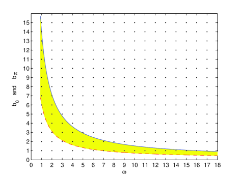
Figure 7: (Color online) Plot of $b_{0}$ and $b_{\pi}$ as a function of $\omega$ for a system with $\gamma=1$, $\Delta=-1$, $c_{0}=2.5$ and a periodic $\delta$-function kick with $c_{1}=0.2$. For each value of $\omega$, the number of even and odd integers lying in the shaded region between $b_{0}$ and $b_{\pi}$ gives the number of Majorana modes at each end of a chain with Floquet eigenvalues equal to $+1$ and $-1$ respectively.

V.2 Analytical results for Majorana end modes in a special case

For the case $\Delta=-\gamma$ and $c_{0}=0$, it turns out that we can analytically find the wave functions of the Majorana end modes. Further, we can explicitly prove that the number of Majorana modes is indeed governed by the quantities $b_{0}$, $b_{\pi}$ and $2c_{1}/\pi$ as discussed above.

We consider a semi-infinite chain in which $n$ goes from 1 to $\infty$ in Eq. (1); we will only discuss the Majorana modes at the left end of this chain. As discussed above, the Floquet operator which performs a time evolution for one time period $T=2\pi/\omega$ consists of a symmetrized product of three steps. The first step evolves from time $t=0$ to $t=\epsilon$ (where $\epsilon$ denotes an infinitesimal quantity), the second step evolves from $t=\epsilon$ to $t=T-\epsilon$, and the third step evolves from $t=T-\epsilon$ to $t=T$. At all times, the Heisenberg operators $a_{n}(t)$ satisfy the equations $da_{n}(t)/dt=i[H(t),a_{n}(t)]$. The first step corresponds to a Hamiltonian

$$H_{1}~{}=~{}\frac{ic_{1}}{2}~{}\delta(t-\frac{\epsilon}{2})~{}\sum_{n=1}^{\infty}~{}a_{2n-1}a_{2n}.$$ (28)

This gives

$$a_{2n-1}(\epsilon) = a_{2n-1}(0)~{}\cos c_{1}~{}+~{}a_{2n}(0)~{}\sin c_{1},$$

$$a_{2n}(\epsilon) = a_{2n}(0)~{}\cos c_{1}~{}-~{}a_{2n-1}(0)~{}\sin c_{1},$$ (29)

for all $n\geq 1$. The second step corresponds to the Hamiltonian

$$H_{0}~{}=~{}i\gamma~{}\sum_{n=1}^{\infty}~{}a_{2n}a_{2n+1}$$ (30)

for $\Delta=-\gamma$ and $c_{0}=0$. (The simple form in Eq. (30) is a special feature of this particular choice of $\gamma$, $\Delta$ and $c_{0}$. For any other choice of these parameters, the Hamiltonian would not decompose into terms involving pairs of different Majorana operators, and the time evolution in this step would not have a simple form). Eq. (30) gives

$$a_{2n}(T-\epsilon) = a_{2n}(\epsilon)~{}\cos(2\gamma T)~{}+~{}a_{2n+1}(\epsilon)~{}\sin(2\gamma T),$$

$$a_{2n+1}(T-\epsilon) = a_{2n+1}(\epsilon)~{}\cos(2\gamma T)~{}-~{}a_{2n}(\epsilon)~{}\sin(2\gamma T),$$

for all $n\geq 1$. Note that $a_{1}(t)$ does not evolve in this step as $H_{0}$ does not contain $a_{1}$; hence $a_{1}(T-\epsilon)=a_{1}(\epsilon)$. Finally, the third step corresponds to the Hamiltonian

$$H_{1}~{}=~{}\frac{ic_{1}}{2}~{}\delta(t-T+\frac{\epsilon}{2})~{}\sum_{n=1}^{\infty}~{}a_{2n-1}a_{2n},$$ (32)

which gives

$$a_{2n-1}(T) = a_{2n-1}(T-\epsilon)~{}\cos c_{1}~{}+~{}a_{2n}(T-\epsilon)~{}\sin c_{1},$$

$$a_{2n}(T) = a_{2n}(T-\epsilon)~{}\cos c_{1}~{}-~{}a_{2n-1}(T-\epsilon)~{}\sin c_{1}.$$

We now discover that the equations above have two solutions for Majorana end modes which correspond to Floquet eigenvalues being equal to $+1$ and $-1$, i.e., with $a_{n}(T)=\pm a_{n}(0)$ respectively for all $n\geq 1$.
(i) For eigenvalues equal to $+1$, we find an unnormalized solution of the form

$$a_{2n-1}(0)=[\tan c_{1}\cot(\gamma T)]^{n}~{}~{}~{}{\rm and}~{}~{}~{}a_{2n}(0)=0$$ (34)

for all $n\geq 1$.
(ii) For eigenvalues equal to $-1$, we find a solution of the form

$$a_{2n-1}(0)=0~{}~{}~{}{\rm and}~{}~{}~{}a_{2n}(0)=[-\cot c_{1}\cot(\gamma T)]^{n}$$ (35)

for all $n\geq 1$.
We see that the wave function $a_{n}(0)$ is real, and the probability $|a_{n}(0)|^{2}$ has a very simple structure; depending on the Floquet eigenvalue, it vanishes for all odd $n$ or all even $n$, while for the other values of $n$ it decreases exponentially as $n$ increases.

Eqs. (34-35) imply that Majorana end modes appear or disappear when $|\tan c_{1}\cot(\gamma T)|$ or $|\cot c_{1}\cot(\gamma T)|$ becomes equal to 1. These are precisely the same conditions as $b_{0}$ or $b_{\pi}$ in Eq. (27) becoming equal to an integer $n$, with Floquet eigenvalue equal to $(-1)^{n}$. We can also explicitly confirm the following result stated above. Namely, we consider all the integers lying between $b_{0}$ and $b_{\pi}$, assuming that $b_{0}$, $b_{\pi}$ and $2c_{1}/\pi$ are not integers. Of these, let $n_{e}^{>}$ ($n_{o}^{>}$) and $n_{e}^{<}$ ($n_{o}^{<}$) respectively denote the numbers of even (odd) integers which are greater than and less than $2c_{1}/\pi$. Then the numbers $N_{+}$ and $N_{-}$ of Majorana modes at the left of the chain with Floquet eigenvalue equal to $+1$ and $-1$ are given by $N_{+}~{}=~{}|n_{e}^{>}-n_{e}^{<}|$ and $N_{-}~{}=~{}|n_{o}^{>}-n_{o}^{<}|$. Interestingly, we find that $N_{\pm}$ can only be equal to 0 or 1 in this case.

V.3 Effect of Time-Reversal Symmetry Breaking

Given a periodically driven time-reversal symmetric system which has Majorana end modes (namely, modes with real eigenvectors and Floquet eigenvalues equal to $\pm 1$ which are separated from all other eigenvalues by a gap), we may ask what would happen if we add small terms which break time-reversal symmetry. We discover that the end modes persist and their Floquet eigenvalues continue to be separated from all other eigenvalues by a gap. However, the Floquet eigenvalues move slightly away from $\pm 1$ in complex conjugate pairs, and the eigenvectors become complex; hence they can no longer be called Majorana modes. This is illustrated in Fig. 8 which shows the Floquet eigenvalues for the modes at each end of the chain for the time-reversal symmetric case given in Eq. (19), while Fig. 9 shows the Floquet eigenvalues for a case with

$$\mu_{n}(t) = c_{0}~{}+~{}c_{1}\sum_{n=-\infty}^{\infty}\delta(t-nT)$$ (36)

$$+~{}c_{2}\sum_{n=-\infty}^{\infty}\delta(t-\frac{T}{4}-nT),$$

which breaks time-reversal symmetry. Although we cannot clearly see from Fig. 9 that the Floquet eigenvalues of the end modes have moved away from $\pm 1$, we have checked numerically that this is so. For a 2800-site system (this is a large enough system size that there is no mixing between the two ends), we find that at each end, the Floquet eigenvalues near $-1$ are given by $-1\pm 0.0015i$ and $-1\pm 0.0037i$, and the eigenvalues near $+1$ are given by $1\pm 0.0007i$ and $1\pm 0.0040i$.

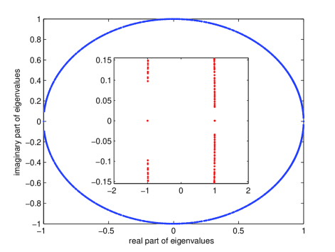
Figure 8: (Color online) Floquet eigenvalues close to $\pm 1$ for a 1000-site system with $\gamma=1$, $\Delta=-1$, $c_{0}=2.5$, and a $\delta$-function kick with $c_{1}=0.2$ at $t=0$ which is repeated with a time period $T=2\pi$. For this time-reversal symmetric case, there are four eigenvalues at exactly $+1$ and $-1$ each, separated by a gap from all other eigenvalues; these are shown more clearly in the inset.

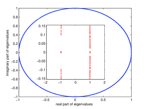
Figure 9: (Color online) Floquet eigenvalues close to $\pm 1$ for a 1000-site system with $\gamma=1$, $\Delta=-1$, $c_{0}=2.5$, and two $\delta$-function kicks with $c_{1}=0.2$ and $c_{2}=0.1$ at $t=0$ and $T/4$ which are repeated with a time period $T=2\pi$. For this case with no time-reversal symmetry, there are four eigenvalues close to but not exactly at $+1$ and $-1$, separated by a gap from all other eigenvalues; these are shown more clearly in the inset.

VI Periodic $\delta$-function Kicks in Hopping and Superconducting Terms

In this section, we will briefly discuss the case where the hopping and superconducting terms in Eq. (1) are given $\delta$-function kicks periodically in time. We will again show that this too can produce Majorana end modes. In particular, we find that there is a Majorana mode at each end of a chain even in the limit of very large driving frequency $\omega$; this is in contrast to the case of periodic $\delta$-function kicks in the chemical potential where there is an upper limit on $\omega$ beyond which there are no Majorana modes. We will limit our discussion to some observations on the Floquet operator and the winding number; we will not consider the possibility of a second topological invariant here.

We consider the case where the chemical potential $\mu$ is independent of time, while

$$\gamma~{}=~{}-\Delta~{}=~{}\gamma_{0}~{}+~{}\gamma_{1}~{}\sum_{n=-\infty}^{\infty}\delta(t-nT).$$ (37)

(As mentioned earlier, this corresponds to an Ising model in a transverse magnetic field, where the Ising interaction $J_{x}$ is given periodic $\delta$-function kicks while the magnetic field does not vary with time). Eqs. (11) and (22) then imply that

$$U_{k}(T,0) = e^{-i\gamma_{1}(\cos k~{}\tau^{z}-\sin k~{}\tau^{y})}$$ (38)

$$\times~{}e^{-i2T[(\gamma_{0}\cos k-\mu)\tau^{z}-\gamma_{0}\sin k~{}\tau^{y}]}$$

$$\times~{}e^{-i\gamma_{1}(\cos k~{}\tau^{z}-\sin k~{}\tau^{y})}.$$

Eq. (38) implies that in the limit $\omega\to\infty$, i.e., $T\to 0$, $U_{k}(T,0)=e^{-i(a_{2,k}\tau^{y}+a_{2,k}\tau^{z})}$, where

$$a_{2,k}~{}=~{}-2\gamma_{1}\sin k~{}~{}~{}~{}{\rm and}~{}~{}~{}~{}a_{3,k}~{}=~{}2\gamma_{1}\cos k.$$ (39)

As $k$ goes from $-\pi$ to $\pi$, this generates a closed curve with winding number $+1$. This implies that there will be one Majorana mode at each end of the chain when $\omega\to\infty$. Numerically, we find that this is indeed the case. We will now prove this analytically for a special set of parameters following a procedure similar to the one followed in Sec. V B.

We consider the case $\gamma_{0}=0$. Considering only the left end of the chain starting from $n=1$ and assuming some initial values of the Heisenberg operators $a_{n}(0)$, we can successively find $a_{n}(\epsilon)$, $a_{n}(T-\epsilon)$ and $a_{n}(T)$ using three sets of evolution equations,

$$a_{2n+1}(\epsilon) = a_{2n+1}(0)~{}\cos\gamma_{1}~{}-~{}a_{2n}(0)~{}\sin\gamma_{1},$$

$$a_{2n}(\epsilon) = a_{2n}(0)~{}\cos\gamma_{1}~{}+~{}a_{2n+1}(0)~{}\sin\gamma_{1},$$ (40)

$$a_{2n-1}(T-\epsilon) = a_{2n-1}(\epsilon)~{}\cos(2\mu T)~{}+~{}a_{2n}(\epsilon)~{}\sin(2\mu T),$$

$$a_{2n}(T-\epsilon) = a_{2n}(\epsilon)~{}\cos(2\mu T)~{}-~{}a_{2n-1}(\epsilon)~{}\sin(2\mu T),$$

and

$$a_{2n+1}(T) = a_{2n+1}(T-\epsilon)~{}\cos\gamma_{1}~{}-~{}a_{2n}(T-\epsilon)~{}\sin\gamma_{1},$$

$$a_{2n}(T) = a_{2n}(T-\epsilon)~{}\cos\gamma_{1}~{}+~{}a_{2n+1}(T-\epsilon)~{}\sin\gamma_{1}.$$

Eqs. (40-LABEL:time3) are valid for all $n\geq 1$. Note that $a_{1}$ does not evolve at all from $t=0$ to $t=\epsilon$ and again from $t=T-\epsilon$ to $t=T$.

We then discover that the above equations have two kinds of solutions.
(i) For Floquet eigenvalue equal to $+1$, i.e., $a_{n}(T)=a_{n}(0)$ for all $n$, we find an unnormalized solution of the form $a_{1}(0)=1$, while $a_{2n+1}=[\tan(\mu T)\cot\gamma_{1}]^{n}/\cos\gamma_{1}$ and $a_{2n}(0)=0$ for all $n\geq 1$. This solution exists if $|\tan(\mu T)\cot\gamma_{1}|<1$. In the limit $T\to 0$, it reduces to $a_{1}(0)=1$ and all other $a_{n}(0)=0$.
(i) For Floquet eigenvalue equal to $-1$, i.e., $a_{n}(T)=-a_{n}(0)$, we find an unnormalized solution of the form $a_{1}(0)=1$, while $a_{2n+1}=[-\cot(\mu T)\cot\gamma_{1}]^{n}/\cos(\gamma_{1})$ and $a_{2n}(0)=0$ for all $n\geq 1$. This solution exists if $|\cot(\mu T)\cot\gamma_{1}|<1$.

VII Simple Harmonic Variation of Chemical Potential with Time

In this section, we discuss the case where the chemical potential varies harmonically with $t$. Namely, the chemical potential in Eq. (3) takes the form

$$\mu(t)~{}=~{}c_{0}~{}+~{}c_{1}\cos(\omega t+\phi).$$ (43)

The Floquet operator can be written as the time-ordered product

$$U(T,0)={\cal T}e^{4\int_{0}^{T}dtM(t)},$$ (44)

where $M(t)$ is an antisymmetric matrix with the non-zero elements

$$(M)_{2n+1,2n} = -~{}(M)_{2n,2n+1}~{}=~{}-\frac{1}{4}(\gamma-\Delta),$$

$$(M)_{2n-1,2n+2} = -~{}(M)_{2n+2,2n-1}~{}=~{}-\frac{1}{4}(\gamma+\Delta),$$

$$(M)_{2n-1,2n} = -~{}(M)_{2n,2n-1}$$ (45)

$$= \frac{1}{2}[c_{0}+c_{1}\cos(\omega t+\phi)].$$

Unlike the case of the periodic $\delta$-function kick, the Floquet operator is no longer a product of only two or three operators; it has to be computed by dividing the time-period $T$ into a large number of time steps of size $\Delta t$ each, and then multiplying $T/\Delta t$ operators in a time-ordered way. Finally, we have to check that the results do not change significantly once $\Delta t$ has been made sufficiently small. Hence this problem takes much more computational time. For the same reason, a numerical calculation of the Floquet operator $U_{k}(T,0)$ takes more time here than the corresponding expression given in Eq. (23) for a periodic $\delta$-function kick. We will not consider the existence of topological invariants here.

Having computed the operator $U(T,0)$, where $T=2\pi/\omega$, we again find all the eigenvalues and eigenvectors of $U(T,0)$ which are also eigenvectors of the parity operator $\cal P$. As functions of the parameters $\gamma$, $\Delta$, $c_{0}$, $c_{1}$, $\phi$, $\omega$ and $N$, we find that the qualitative features of the Majorana end modes that we find are similar to the case of the periodic $\delta$-function kicks. As before, we find that end modes can appear even when the chemical potential places the corresponding time-independent system in a non-topological phase at all times $t$.

The effect of the phase $\phi$ in Eqs. (43) and (45) turns out to be interesting. The Floquet operator $U(T,0)$, now denoted by $U_{\phi}(T,0)$, clearly depends on $\phi$. However, we can show that the eigenvalues of $U_{\phi}(T,0)$ are independent of $\phi$ soori . To see this, note that a shift in the phase $\phi$ by an amount $\delta$ is equivalent to a shift in time by the amount $\delta/\omega$. Hence

$$U_{\phi}(T,0) = U_{0}(T+\phi/\omega,\phi/\omega)$$ (46)

$$= U_{0}(T+\phi/\omega,T)U_{0}(T,\phi/\omega)$$

$$= U_{0}(T+\phi/\omega,T)U_{0}(T,0)U_{0}^{-1}(\phi/\omega,0)$$

$$= U_{0}(\phi/\omega,0)U_{0}(T,0)U_{0}^{-1}(\phi/\omega,0),$$

where we have used the fact that $U_{0}(T+\phi/\omega,T)=U_{0}(\phi/\omega,0)$. Eq. (46) shows that $U_{\phi}(T,0)$ is related to $U_{0}(T,0)$ by a unitary transformation involving $U_{0}(\phi/\omega,0)$; hence they have the same eigenvalues while their eigenvectors are related by the same unitary transformation. This also implies that studying how an eigenvector corresponding to a particular eigenvalue of $U_{\phi}(T,0)$ changes with $\phi$ is equivalent to studying how that eigenvector changes with time under evolution with $U_{0}(t=\phi/\omega,0)$.

The effect of a phase change on the wave functions of the Majorana end modes can sometimes be quite dramatic. We consider a 100-site system with $\gamma=1$, $\Delta=-1$, $c_{0}=2.5$, $c_{1}=0.3$ and $\omega=14$. Figs. 10 and 11 show the probabilities of the two end modes for $\phi=0$ and $\pi/2$ respectively; equivalently, we can think of these figures as showing the effect of evolving the end modes by a time of $T/4$. We see that the detailed form of the end mode wave functions are quite different in the two cases. For $\phi=0$, the wave function $a_{m}$ of the mode at the left (right) end is non-zero only if $m$ is even (odd). For $\phi=\pi/2$, both end modes have wave functions in which $a_{m}$ is non-zero for both even and odd values of $m$.

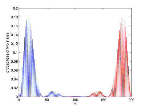
Figure 10: (Color online) Plot of the probabilities of the two end states for a 100-site system with $\gamma=1$, $\Delta=-1$, $c_{0}=2.5$, and a simple harmonic driving with $c_{1}=0.3$, $\omega=14$ and $\phi=0$.

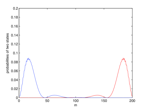
Figure 11: (Color online) Plot of the probabilities of the two end states for a 100-site system with $\gamma=1$, $\Delta=-1$, $c_{0}=2.5$, and a simple harmonic driving with $c_{1}=0.3$, $\omega=14$ and $\phi=\pi/2$.

VIII Effects of electron-phonon interactions and noise on Majorana end modes

An important question relevant to the experimental detection of Majorana end modes generated by periodic driving is whether such modes are stable under perturbations which do not have the same periodicity as the driving term. For instance, at finite temperature, there will be phonons with a range of frequencies $\omega^{\prime}$, and we may be interested in effect of electron-phonon interactions on the Majorana end modes. We may also be interested in the effect of a random noise in some of the parameters in the Hamiltonian. We will discuss both these questions here.

Given a Majorana mode produced by driving with a frequency $\omega$, let us define the quasienergy gap as $\Delta E=\omega\Delta\theta/(2\pi)$, where $\Delta\theta$ is the gap between the Floquet eigenvalues of the bulk modes (which are of the form $e^{i\theta}$) and the Majorana mode (which must have $e^{i\theta}=\pm 1$, i.e., $\theta=0$ or $\pi$). It has been shown in Ref. kita2, that the Majorana mode will survive if the phonon frequencies $\omega^{\prime}$ (which are mainly governed by the temperature) are much smaller than the gap $\Delta E$ and the driving frequency $\omega$ is much larger than both $\omega^{\prime}$ and the bandwidth. The basic argument for this result is that the driving with frequency $\omega$ and an interaction between an electron and a phonon with frequency $\omega^{\prime}$ can combine to produce transitions between two states whose energies differ by $\omega^{\prime}+n\omega$, where $n$ is an integer. (We are assuming here that the electron-phonon interaction is small so that only one-phonon processes are important). If $n=0$, then we cannot have a transition between the Majorana mode and a bulk mode if $\omega^{\prime}\ll\Delta E$. On the other hand, if $n\neq 0$, then $\omega^{\prime}+n\omega$ is much larger than the bandwidth; then there is no bulk mode available to which we can make a transition from the Majorana mode.

Applied to our model, the argument outline above implies that if $\omega$ is much larger than the bandwidth of the time-independent part of the Hamiltonian (this is equal to $4|\gamma+c_{0}|$ as we can show using Eq. (12)), a Majorana mode will survive if the phonon frequencies are much smaller than the corresponding quasienergy gap $\Delta E$. Conversely, if $\omega$ is of the order of or smaller than the bandwidth, then the Majorana mode may not be stable against electron-phonon interactions. The large number of Majorana modes that we found in Sec. V A for very small values of $\omega$ may therefore not be stable against electron-phonon interactions.

We have numerically also studied what happens when the chemical potential has a term which is uniform in space but varies randomly in time; in addition, the chemical potential is given periodic $\delta$-function kicks. We compute the Floquet operator by dividing the total time $\bar{T}$ into a large number of steps (of size $\Delta\bar{T}$ each) and multiplying the time evolution operators over all the steps in a time-ordered way. We consider a chain with $\gamma=1$, $\Delta=-1$, $c_{0}=2.5$, $c_{1}=0.2$, with a range of system sizes from 200 to 1000 and a range of frequencies $\omega$ from 1 to 16. To study the effect of noise, we add a term to the chemical potential $\mu(t)$ which is of the form $rp(t)$, where $p(t)$ is a random variable which is uniformly distributed from $-1$ to $1$ and is uncorrelated at different times (this is achieved by choosing $p(t)$ to be a different random number at each time step of our numerical calculations), and $r$ is the coefficient of the random term. We have studied the effect of the noise over a total time $\bar{T}$ ranging from $T$ to $11T$, where $T=2\pi/\omega$. (This implies that our noise has a period varying from $T$ to $11T$, rather than being truly aperiodic). We find that for $4\leq\omega\leq 16$, the Majorana end modes survive up to a value of $r$ which is about $0.3$. For smaller values of $\omega=2,3$, the Majorana modes survive up to a value of $r$ of about $0.05$, while for $\omega=1$, they survive up to $r$ of about $0.025$. The critical value of $r$ varies somewhat from one run to another as is expected for a random noise. (We have not studied how $r$ depends on the quasienergy gap $\omega\Delta\theta/(2\pi)$; note that this gap also generally decreases as $\omega$ decreases). To conclude, a noise in the chemical potential does not destroy the Majorana modes if the strength of the noise is less than some value which decreases with the driving frequency $\omega$.

We note that electron-phonon interactions and noise do not have the same effects in our system. The random noise that we have considered contains terms with a very large number of frequencies ranging from $2\pi/\bar{T}$ to $2\pi/\Delta\bar{T}$, and all these terms interact with the electrons. On the other hand, we have only considered processes in which only one phonon interacts with the electrons and each phonon has a single frequency $\omega^{\prime}$. The electron-phonon interactions and noise therefore affect the Majorana modes in different ways.

IX Conclusions

In this work we have shown that periodic driving of a one-dimensional model of electrons with $p$-wave superconductivity or a spin-1/2 $XY$ chain in a transverse magnetic field can generate Majorana modes at the ends if we have a large and open system which is time-reversal symmetric. To simplify the calculations, we have mainly studied the case in which the chemical potential of the electrons (or the transverse magnetic field in the spin language) is given a periodic $\delta$-function kick. However, similar results are found when the chemical potential (or magnetic field) is driven in a simple harmonic way, or when the hopping and superconducting terms are given periodic $\delta$-function kicks.

The Majorana end modes exist only for very large system sizes and have three characteristic features: the Floquet eigenvalues are exactly equal to $\pm 1$, they are separated from all the other eigenvalues by a finite gap, and the wave functions are real. If the system is not time-reversal symmetric, we find that there may still be end modes whose eigenvalues are separated from all the others by a finite gap may; however, the eigenvalues are no longer exactly at $\pm 1$, and the wave functions are not real. Hence these cannot be called Majorana modes.

In analogy with the known topological invariants which predict the number of zero energy Majorana end modes for a system with a time-independent Hamiltonian, we have studied if the driven system has topological invariants which can correctly predict the number of end modes. We have shown that there are two topological invariants which work for a wide range of the driving frequency $\omega$ for the case of the periodic $\delta$-function kick. The first invariant is a winding number which is similar in form to the topological invariant for a time-independent Hamiltonian with time-reversal symmetry; this invariant sometimes, but not always, gives the total number of end modes. The second invariant is superior in that it separately gives us the numbers of end modes with Floquet eigenvalues equal to $+1$ and $-1$ for all values of the parameters. The second invariant also gives us a simple condition which can predict the values of $\omega$ at which end modes appear or disappear.

We have studied the effects of some experimentally relevant perturbations such as electron-phonon interactions and a random noise on the Majorana end modes. We generally find that the Majorana modes become more robust as the driving frequency $\omega$ increases.

Recently there has been considerable excitement over claims of the detection of Majorana modes in semiconducting/superconducting nanowires kouwenhoven ; deng ; rokhinson ; das ; finck following some theoretical proposals lutchyn1 ; oreg ; alicea ; stanescu . A zero bias peak has been observed in the tunneling conductance into one end of the nanowire, and it has been suggested that this is the signature of a Majorana end mode. Our results can be tested in similar systems by applying a gate voltage to the nanowire which varies periodically in time in some way. One would like to see if such a time-dependent gate voltage can give rise to a zero bias peak; this has recently been studied in Ref. kundu, . An important question which needs to be investigated in this context is how the Majorana end modes appear in the steady state after the oscillatory part of the gate voltage is switched on. This would require a treatment of various relaxation mechanisms which may be present in the system lind1 . Finally, the effects that disorder in the chemical potential motrunich ; brouwer1 ; lobos ; cook ; pedrocchi and electron-electron interactions ganga ; lobos ; lutchyn2 ; fidkowski2 have on the Majorana end modes also need to be examined.

References

- (1)
- (2) M. Z. Hasan and C. L. Kane, Rev. Mod. Phys. 82, 3045 (2010).
- (3) X.-L. Qi and S.-C. Zhang, Rev. Mod. Phys. 83, 1057 (2011).
- (4) L. Fidkowski and A. Kitaev, Phys. Rev. B 83, 075103 (2011).
- (5) T. Kitagawa, E. Berg, M. Rudner, and E. Demler, Phys. Rev. B 82, 235114 (2010).
- (6) N. H. Lindner, G. Refael, and V. Galitski, Nature Phys. 7, 490 (2011).
- (7) L. Jiang, T. Kitagawa, J. Alicea, A. R. Akhmerov, D. Pekker, G. Refael, J. I. Cirac, E. Demler, M. D. Lukin, and P. Zoller, Phys. Rev. Lett. 106, 220402 (2011).
- (8) Z. Gu, H. A. Fertig, D. P. Arovas, and A. Auerbach, Phys. Rev. Lett. 107, 216601 (2011).
- (9) T. Kitagawa, T. Oka, A. Brataas, L. Fu, and E. Demler, Phys. Rev. B 84, 235108 (2011).
- (10) N. H. Lindner, D. L. Bergman, G. Refael, and V. Galitski, Phys. Rev. B 87, 235131 (2013).
- (11) M. Trif and Y. Tserkovnyak, Phys. Rev. Lett. 109, 257002 (2012).
- (12) A. Russomanno, A. Silva, and G. E. Santoro, Phys. Rev. Lett. 109, 257201 (2012).
- (13) V. M. Bastidas, C. Emary, G. Schaller, and T. Brandes, Phys. Rev. A 86, 063627 (2012).
- (14) V. M. Bastidas, C. Emary, B. Regler, and T. Brandes, Phys. Rev. Lett. 108, 043003 (2012).
- (15) M. Tomka, A. Polkovnikov, and V. Gritsev, Phys. Rev. Lett. 108, 080404 (2012).
- (16) A. Gomez-Leon and G. Platero, Phys. Rev. B 86, 115318 (2012), and Phys. Rev. Lett. 110, 200403 (2013).
- (17) B. Dóra, J. Cayssol, F. Simon, and R. Moessner, Phys. Rev. Lett. 108, 056602 (2012).
- (18) D. E. Liu, A. Levchenko, and H. U. Baranger, Phys. Rev. Lett. 111, 047002 (2013).
- (19) Q.-J. Tong, J.-H. An, J. Gong, H.-G. Luo, and C. H. Oh, Phys. Rev. B 87, 201109(R) (2013).
- (20) M. S. Rudner, N. H. Lindner, E. Berg, and M. Levin, Phys. Rev. X 3, 031005 (2013).
- (21) J. Cayssol, B. Dóra, F. Simon, and R. Moessner, Phys. Status Solidi RRL 7, 101 (2013).
- (22) Y. T. Katan and D. Podolsky, Phys. Rev. Lett. 110, 016802 (2013).
- (23) A. Kundu and B. Seradjeh, arXiv:1301.4433v2, to appear in Phys. Rev. Lett.
- (24) V. M. Bastidas, C. Emary, G. Schaller, A. Gómez-León, G. Platero, and T. Brandes, arXiv:1302.0781.
- (25) T. L. Schmidt, A. Nunnenkamp, and C. Bruder, New J. Phys. 15, 025043 (2013).
- (26) A. A. Reynoso and D. Frustaglia, Phys. Rev. B 87, 115420 (2013).
- (27) C.-C. Wu, J. Sun, F.-J. Huang, Y.-D. Li, and W.-M. Liu, arXiv:1306.3870.
- (28) M. C. Rechtsman, J. M. Zeuner, Y. Plotnik, Y. Lumer, S. Nolte, M. Segev, and A. Szameit, arXiv:1212.3146.
- (29) E. Lieb, T. Schultz, and D. Mattis, Ann. Phys. (NY) 16, 407 (1961).
- (30) H.-J. Stöckmann, Quantum Chaos (Cambridge University Press, Cambridge, 1999).
- (31) W. DeGottardi, D. Sen, and S. Vishveshwara, New J. Phys. 13, 065028 (2011).
- (32) W. DeGottardi, M. Thakurathi, S. Vishveshwara, and D. Sen, arXiv:1303:3304, to appear in Phys. Rev. B.
- (33) Y. Niu, S. B. Chung, C.-H. Hsu, I. Mandal, S. Raghu, and S. Chakravarty, Phys. Rev. B 85, 035110 (2012).
- (34) A. Kitaev, Physics-Uspekhi 44, 131 (2001), arXiv:cond-mat/0010440v2 (2000).
- (35) A. Soori and D. Sen, Phys. Rev. B 82, 115432 (2010).
- (36) V. Mourik, K. Zuo, S. M. Frolov, S. R. Plissard, E. P. A. M. Bakkers, and L. P. Kouwenhoven, Science 336, 1003 (2012).
- (37) M. T. Deng, C. L. Yu, G. Y. Huang, M. Larsson, P. Caroff, and H. Q. Xu, Nano Lett. 12, 6414 (2012).
- (38) L. P. Rokhinson, X. Liu, and J. K. Furdyna, Nature Phys. 8, 795 (2012).
- (39) A. Das, Y. Ronen, Y. Most, Y. Oreg, M. Heiblum, and H. Shtrikman, Nature Phys. 8, 887 (2012).
- (40) A. D. K. Finck, D. J. Van Harlingen, P. K. Mohseni, K. Jung, and X. Li, Phys. Rev. Lett. 110, 126406 (2013).
- (41) R. M. Lutchyn, J. D. Sau, S. Das Sarma, Phys. Rev. Lett. 105, 077001 (2010).
- (42) Y. Oreg, G. Refael, and F. von Oppen, Phys. Rev. Lett. 105, 177002 (2010).
- (43) J. Alicea, Rep. Prog. Phys. 75, 076501 (2012).
- (44) T. D. Stanescu and S. Tewari, J. Phys.: Condens. Matter 25, 233201 (2013).
- (45) O. Motrunich, K. Damle, and D. A. Huse, Phys. Rev. B 63, 224204 (2001).
- (46) P. W. Brouwer, M. Duckheim, A. Romito, and F. von Oppen, Phys. Rev. Lett. 107, 196804 (2011).
- (47) A. M. Cook, M. M. Vazifeh, and M. Franz, Phys. Rev. B 86, 155431 (2012).
- (48) F. L. Pedrocchi, S. Chesi, S. Gangadharaiah, and D. Loss, Phys. Rev. B 86, 205412 (2012).
- (49) A. M. Lobos, R. M. Lutchyn, and S. Das Sarma, Phys. Rev. Lett. 109, 146403 (2012).
- (50) S. Gangadharaiah, B. Braunecker, P. Simon, and D. Loss, Phys. Rev. Lett. 107, 036801 (2011).
- (51) R. M. Lutchyn and M. P. A. Fisher, Phys. Rev. B 84, 214528 (2011).
- (52) L. Fidkowski, J. Alicea, N. H. Lindner, R. M. Lutchyn, and M. P. A. Fisher, Phys. Rev. B 85, 245121 (2012).