Continuous third harmonic generation in a terahertz driven modulated nanowire

Abstract

We consider the possibility of observing continuous third-harmonic generation using a strongly driven, single-band one-dimensional metal. In the absence of scattering, the quantum efficiency of frequency tripling for such a system can be as high as 93%. Combining the Floquet quasi-energy spectrum with the Keldysh Green’s function technique, we derive the semiclassical master equation for a one-dimensional band of strongly and rapidly driven electrons in the presence of weak scattering by phonons. The power absorbed from the driving field is continuously dissipated by phonon modes, leading to a quasi-equilibrium in the electron distribution. We use the Kronig-Penney model with varying effective mass to establish growth parameters of an InAs/InP nanowire near optimal for third harmonic generation at terahertz frequency range.

1 Introduction

When electrons in a crystal band are driven by an external time-independent electric field, they move periodically across the Brillouin zone, creating characteristic Bloch oscillations^{1, 2, 3, 4, 5}. The frequency of the oscillations, $\omega_{\mathrm{B}}=eEa/\hbar$, where $a$ is the unit cell size, coincides with the energy separation between neighboring states localized on a Wannier-Stark ladder ^{5, 6}. The effect has been observed for electrons/holes in semiconducting superlattices^{7, 8}, for atoms trapped in a periodic optical potential⁹, and for light propagating in a periodic array of waveguides, with gradient of the temperature or of the refraction index working as an effective electric field^{10, 11, 12}.

Combining the effects of a strong, time-periodic driving field, with the nonlinearity of the Bloch oscillations leads to higher harmonic generation of the driving frequency^{13, 14, 15}. This effect has recently been observed in bulk ZnO crystals strongly driven by a few-cycle pulsed infrared laser¹⁶. The application of the infrared field in short, 100-femtosecond, pulses was necessary to ensure that the absorbed energy could be transferred to the lattice and dissipated.

In this work, we suggest that frequency multiplication due to periodically-driven Bloch oscillations could also be observed in a steady-state setting, e.g., a periodically modulated nanowire (or an array of such nanowires) continuously driven by high-amplitude terahertz radiation (see Fig. 1). In the weak-scattering limit, the quantum efficiency of frequency tripling for such a system can be as high as 93%.

For a nanowire in mechanical contact with an insulating, optically transparent substrate, a quasi-equilibrium electron distribution will be reached as the power absorbed from the driving field will be continuously dissipated into phonon modes. This distribution can be quite different from the initial, equilibrium Fermi distribution. In particular, at the driving field amplitude which is optimal for third harmonic generation, the distribution can be both broadened and inverted. The inversion of the distribution occurs once the driving field amplitude exceeds the dynamical localization threshold^{17, 18}.

Figure 1: (a) A nanowire made with alternating InAs/InP regions. (b), (c) Schematic of the third harmonic generation with a planar array of such nanowires. The driving field is $s$-polarized so that the electric field $E_{1}$ be parallel to the nanowires. The generated third harmonic will have the same polarization but propagate at a different angle.

In our analytic derivation, we combine the Floquet quasi-energy description with the Keldysh Green’s function technique to obtain the semiclassical master equation for a one-dimensional band of strongly and rapidly driven electrons in the presence of weak scattering by phonons. We solve these equations numerically to find the electron distribution function for a cosine energy band at a given driving field frequency (fixed at $\Omega/2\pi=1$ THz) and the field amplitude chosen to suppress the generation of the principal harmonic. This electron distribution is used as an input for calculating the time-dependent current and the intensity radiated at different harmonics of the driving field frequency. We use these results to find the optimal dimensions of a periodically modulated InAs/InP nanowire, which would yield the most efficient frequency tripling of $1$ THz radiation.

2 Theoretical approach

We consider a single-band one-dimensional metallic wire driven by a harmonic electric field with the amplitude $E_{0}$ and frequency $\Omega$, and coupled to substrate phonons,

$$H=H_{0}+H_{\mathrm{e-ph}}+H_{\mathrm{ph}},$$ (1)

where the electron, electron-phonon, and phonon Hamiltonians are, respectively

$$H_{0} = \sum_{k}\varepsilon\biglb(k+A(t)\bigrb)c_{k}^{\dagger}c_{k},$$ (2)

$$H_{\mathrm{e-ph}} = V^{-1/2}\sum_{\mathbf{q},k}{M_{{\bf q},k}}c_{k+q_{\parallel}}^{\dagger}c_{k}(b_{\bf q}+b_{-\bf q}^{\dagger}),$$ (3)

$$H_{\rm ph} = \sum_{\bf q}\omega_{\bf q}b_{\bf q}^{\dagger}b_{\bf q}.$$ (4)

Here $c_{k}$ $(c_{k}^{\dagger})$ is the annihilation (creation) operator for an electron with one-dimensional momentum $\hbar k$ and energy $\varepsilon(k)$. To apply our results to a periodically modulated nanowire, we assume a tight-binding model with the electronic spectrum,

$$\varepsilon(k)=-2J\cos(ka),$$ (5)

where $J$ is the hopping matrix element and $a$ is the period of the potential along the chain. The electric field is incorporated into the Hamiltonian through the vector potential $A(t)=A_{0}\sin\Omega t$ with $A_{0}=eE_{0}/\hbar\Omega$ representing the vector potential of the driving field. Phonon annihilation (creation) operators $b_{\mathbf{q}}$ and $b_{\mathbf{q}}^{\dagger}$ are labeled with the three-dimensional wavevector $\mathbf{q}\equiv(q_{\parallel},\mathbf{q}_{\perp})$ and $\omega_{\mathbf{q}}$ is the phonon frequency (electron spin and phonon branch indices are suppressed). The factors $M_{{\bf q},k}=\alpha_{\mathbf{q},k}(\hbar/2\omega_{\mathbf{q}})^{1/2}$ are the matrix elements for electron-phonon scattering.

We ignore the effects of disorder or electron-electron interactions, and consider lattice phonons in thermal equilibrium at temperature $\hbar/k_{B}\beta$. We do not include directly the scattering by phonon modes of the nanowire, assuming that they are strongly hybridized with those of the substrate, with the corresponding effects incorporated in the matrix elements $M_{\mathbf{q},k}$. The electron-phonon coupling is considered to be weak, meaning that the phonon scattering time is long compared to the period $\tau\equiv 2\pi/\Omega$ of the driving field.

2.1 Modified energy spectrum of the driven system

The dynamics of the strongly-driven electrons with the Hamiltonian (2) is characterized by non-monotonous phases

$$\varphi_{k}(t)=\int_{0}^{t}dt^{\prime}\varepsilon\biglb(k+A(t^{\prime})\bigrb).$$ (6)

The phase accumulated over a period, $\varphi_{k}(\tau)$, can be expressed in terms of the average particle energy with the momentum $\hbar k$,

$$\langle\varepsilon(k+A)\rangle\equiv{\tau}^{-1}\int_{0}^{\tau}dt\,\varepsilon\biglb(k+A(t)\bigrb);$$ (7)

clearly, this energy can be also identified as the Floquet energy of a single-electron state. While Eq. (7) does not include the usual additive uncertainty $m\Omega$, this particular choice has the advantage that in the weak-field limit, $A_{0}\to 0$, $\langle\varepsilon(k+A)\rangle$ recovers the zero-field spectrum $\varepsilon(k)$.

The average energy (7) also coincides with that introduced in the theory of dynamical localization^{17, 18}. Dynamical localization occurs when the effective band becomes flat, i.e., $\langle\varepsilon(k+A)\rangle\to 0$. The corresponding condition is most easily obtained in the special case of tight-binding model with the spectrum (5),

$$\langle\varepsilon(k+A)\rangle=-2\widetilde{J}\cos(ka),\quad\widetilde{J}\equiv J\,J_{0}(A_{0}a),$$ (8)

where $J_{0}(z)$ is the zeroth order Bessel function. With the driving field amplitude increasing from zero the bandwidth is gradually reduced; it switches sign at the roots of the Bessel function, $A_{0}\,a=\zeta_{0n}$. The first time this happens corresponds to the electric field $E_{0}=\zeta_{01}\hbar\Omega/ea$, where $\zeta_{01}\approx 2.405$.

2.2 Frequency Multiplication with weak scattering

We obtain the instantaneous current by averaging the canonical velocity operator $\partial H/\partial A$ over the electron distribution function $f_{k}\equiv\langle c_{k}^{\dagger}c_{k}\rangle$,

$$i(t)=C_{f}(t)\,\sin A(t)a+S_{f}(t)\,\cos A(t)a,$$ (9)

where we assumed the tight-binding spectrum (5) and used the definitions

$$C_{f}(t)\equiv 2J\int\frac{dk}{2\pi}\cos(k)f_{k},\quad S_{f}(t)\equiv 2J\int\frac{dk}{2\pi}\sin(k)f_{k}.$$ (10)

In the limit of weak scattering, the distribution function $f_{k}$ is time- independent and always symmetric, $f_{-k}=f_{k}$. Thus, $S_{f}(t)=0$ while $C_{f}(t)=C_{f}$ is a time-independent pre-factor. The Fourier components of the current are obtained directly,

$$i(t)=2C_{f}\sum_{m=1,3,5,\ldots}J_{m}(A_{0}a)\sin(m\Omega t),$$ (11)

where the summation is over the odd harmonics $m$. By choosing $A_{0}a=\zeta_{11}\approx 3.8317$, the first harmonic can be fully suppressed, which leaves the third harmonic dominant. The maximal value for the fraction of the energy emitted into the third harmonic ($93.34\%$) is found in close vicinity of this amplitude, see Fig. 2.

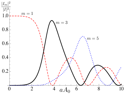
Figure 2: Normalized magnitude squared of the Fourier harmonics of the instantaneous current, $|I_{m}|^{2}$, for $m=1$ (red dashed), $m=3$ (black, solid), and $m=5$ (blue, dotted) plotted as a function of the dimensionless amplitude of the vector potential of the driving field, see Eq. (2). The intensities $|I_{m}|^{2}$ correspond to the power emitted in the corresponding harmonics when multiple nanowires are used in a planar geometry, see Fig. 1 (b),(c).

2.3 Transition kinetics in a driven system

We use the Keldysh non-equilibrium Green’s function (GF) formalism^{19, 20, 21, 22} along with a perturbation theory expansion with respect to the entire time-dependent electron Hamiltonian (2); the corresponding evolution is solved exactly in terms of the phases (6). Previously, related approaches have been used, e.g., for describing ionization of atoms^{23, 24} and the high-order harmonic generation²⁵ in the field of ultrashort laser pulses. Here, instead of solving the corresponding equations numerically, we take the limit of weak electron-phonon coupling and analytically derive the semiclassical master equation for electron distribution function averaged over the period of the driving field, see Eqs. (17) and (18). The same master equation can also be derived from the formalism by Konstantinov and Perel’²⁶ with the help of an appropriate resummation of the perturbation series²⁷.

In the interaction representation with respect to the time-dependent Hamiltonian (2), the electron operators acquire time-dependence $e^{-i\varphi_{k}(t)}c_{k}$ with quasiperiodic phases (6). We separate these phases by defining the “lower-case” GFs

$$g_{k}(t_{2},t_{1})=e^{-i\varphi_{k}(t_{2})}G_{k}(t_{2},t_{1})e^{i\varphi_{k}(t_{1})},$$ (12)

where the “upper-case” $G_{k}(t_{2},t_{1})$ is any of the conventional GFs introduced in the Keldysh formalism^{19, 20, 21, 22}. These phases introduce rapid oscillations in the self-energy, making the direct Wigner transformation difficult. We notice, however, that in the limit of weak electron-phonon coupling, the GFs (12) are expected to change only weakly when both time arguments are incremented by the driving period $\tau$. This implies that in the following decomposition,

$$g_{k}(t_{2},t_{1})=\sum_{m}g_{k,m}(t,T)e^{-im\Omega T},$$ (13)

$t\equiv t_{2}-t_{1}$ is the “fast” time, while $T\equiv(t_{2}+t_{1})/2$ is the “slow” time when it appears as an argument of thus defined Floquet components $g_{k,m}(t,T)$ of the GF. The Dyson equations for thus defined Keldysh $g_{k,m}^{K}$ and retarded $g_{k,m}^{R}$ GFs²⁰ have the form

$$(i\partial_{T}+m\Omega)g_{k,m}^{K}(t,T) = I^{K}_{\mathrm{coll}},$$ (14)

$$i\partial_{t}g_{k,m}^{R}(t,T) = \delta_{m,0}\,\delta(t)+I^{R}_{\mathrm{coll}},$$ (15)

where $I^{K}_{\mathrm{coll}}$ and $I^{R}_{\mathrm{coll}}$ are the collision integrals originating from the corresponding self-energy functions. The collision integrals being relatively small, both $g_{k,m}^{K}$ and $g_{k,m}^{R}$ are dominated by the $m=0$ components²⁸.

To derive the semiclassical master equation, we write the equations for the $m=0$ components of the “lesser” $g^{<}$ and “greater” $g^{>}$ GFs²⁰, perform the Wigner transformation replacing the fast time variable $t$ by the frequency $\omega$, and use a version of the Kadanoff-Baym approximation²⁹

$$g^{<}_{k,0}(\omega,T)=iA_{k,0}(\omega,T)f_{k}(T),\quad A_{k,0}(\omega)\approx\delta(\omega),$$ (16)

for the corresponding spectral function, $A_{k,0}(\omega,T)=i[g^{<}_{k,0}(\omega,T)-g^{>}_{k,0}(\omega,T)]=2\,{\Im\rm m}\mathop{g}^{R}_{k,0}(\omega,T)$, where $f_{k}(T)$ is the non-equilibrium electron distribution function averaged over the period. This requires that the electron-phonon coupling be weak, and assumes that the electron spectrum renormalization has been included in the Hamiltonian (2).

The resulting master equation for weak electron-phonon interactions has the following standard form²⁸

$$\frac{d}{dt}{f}_{k}(T) = \int\frac{dk^{\prime}}{2\pi}\Bigl{\{}\Gamma_{k,k^{\prime}}\,[1-f_{k^{\prime}}(T)]f_{k}(T)$$ (17)

$$\qquad\;\;-\Gamma_{k^{\prime},k}\,f_{k^{\prime}}(T)[1-f_{k}(T)]\Bigr{\}},$$

where the transition rates are

$$\Gamma_{k,k^{\prime}} = 2\sum_{m}|S_{k,k^{\prime}}(m)|^{2}\int_{0}^{\infty}\!\!\!{d\omega}\,W_{k,k^{\prime}}(\omega)$$ (18)

$$\hskip-32.52127pt\times\left[(n_{\omega}+1)\delta(\Delta\varepsilon_{k,k^{\prime}}^{(m)}-\hbar\omega)+n_{\omega}\delta(\Delta\varepsilon_{k,k^{\prime}}^{(m)}+\hbar\omega)\right].\;\;$$

Here $W_{k,k^{\prime}}(\omega)$ is the phonon spectral function (density of states weighted by the square of the coupling) for a given momentum $q_{\parallel}=k^{\prime}-k$ along the wire, see Eq. (3), $n_{\omega}\equiv[\exp(\beta\omega)-1]^{-1}$ is the phonon distribution function, and the energy increment

$$\Delta\varepsilon_{k,k^{\prime}}^{(m)}\equiv\langle\varepsilon(k+A)\rangle-\langle\varepsilon(k^{\prime}+A)\rangle-m\,\hbar\Omega,$$ (19)

is the energy carried in or out by phonons, depending on its sign. Note that this energy includes $m$ quanta of the driving field, emitted or absorbed, depending on the sign of $m=0,\pm 1,\ldots$. The matrix elements $S_{k,k^{\prime}}(m)$ are the Fourier expansion coefficients of the product of the two phase factors, $e^{i\delta\varphi_{k}(t)-i\delta\varphi_{k^{\prime}}(t)}$, where $\delta\varphi_{k}(t)\equiv\varphi_{k}(t)-t\langle\varepsilon(k+A)\rangle$ is the periodic part of the phase. They satisfy the sum rule

$$\sum_{m=-\infty}^{\infty}|S_{k,k^{\prime}}(m)|^{2}=1.$$ (20)

Clearly, the equilibrium Fermi distribution for $f_{k}$ is only obtained in the limit of small electric field amplitudes, such that $S_{k,k^{\prime}}(m)$ with $m=0$ gives the dominant contribution.

3 Simulation results

The results presented in this section have been obtained by numerically finding the stationary solution of the discretized version of the master equation (17) with transition rates (18). A simple model for the phonon spectral function, $W_{k,k^{\prime}}(\omega)=\gamma^{2}\,\theta(\omega-s\left|k-k^{\prime}\right|)$, was used, with the sound speed $s=5\times 10^{3}$ m/s as appropriate for typical 3D acoustical phonons. Since we assume no other scattering mechanisms, the quasi-equilibrium distribution functions $f_{k}$ and other results do not depend on the magnitude of the electron-phonon coupling $\gamma^{2}$.

We fix the phonon temperature at $4.2$K, the lattice period $a=8.64$ nm, the average electron filling at $1/2$ and choose the driving field frequency $\Omega/2\pi=10^{12}$ Hz (energy $\hbar\Omega\approx 4.14$ meV). Also, the amplitude $A_{0}a=\zeta_{11}\approx 3.8317$ is fixed, which corresponds to the point where the first harmonic generation is fully suppressed [see Fig. 2]. At this point the effective coupling is $\widetilde{J}=J\,J_{0}(\zeta_{11})\approx-0.403\,J$, which creates an inverted and somewhat narrowed band. The effective bandwidth is smaller than $\hbar\Omega$ for $J<2.57$ meV.

In Fig. 3, we show the intensity $|I_{3}|^{2}$ of the radiated third harmonic (in arbitrary units) as a function of the tight-binding hopping parameter $J$. The overall upward trend reflects the linear scaling of the current with $J$. The plot has a series of pronounced maxima and minima related to the structure of the distribution function $f_{k}$, see Fig. 4. Indeed, at the first maximum of the radiated intensity $|I_{3}|^{2}$, $J=2.7$ meV, the distribution function has a well-defined minimum at $k=0$ and symmetric maxima at $k=\pm\pi/a$ [Fig. 4(b)]; notice the population inversion consistent with negative $\widetilde{J}$. On the other hand, the distribution in Fig. 4(c) corresponding to the first minimum of radiated intensity, $J=4.5$ meV, is much flatter. This flattening can be traced to a sharp increase of the transition rates connecting the regions of momentum space near $k=0$ and $k=\pi/a$. This is illustrated in Fig. 5, where transition rates between $k=0$ and $k=\pi/a$ are shown. The corresponding phases $\delta\varphi_{\pi/a}=-\delta\varphi_{0}$ have only even harmonics $m\Omega$, $m=2,4,\ldots$, and the threshold values of $J$ for different $m$ correspond to sharp maxima of $\Gamma_{0,\pi/a}$.

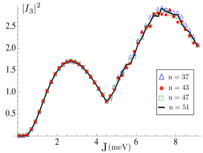
Figure 3: Magnitude squared of the third harmonic of the instantaneous current (arbitrary units), plotted as a function of the tight-binding parameter $J$, computed with $N_{k}=37,43,47,51$ discrete momentum points as indicated in the caption. See text for other simulation parameters. The pronounced minima are caused by the flattening of the distribution function near thresholds of $m$-photon-assisted scattering between the vicinities of $k=0$ and $k=\pm\pi/a$, with $m$ even.

In Fig. 6, we show how the average power ${\cal P}$ radiated into the phonon modes scales with the tight-binding parameter $J$. While general dependence on $J$ is monotonic, at $J=4.5$ meV, where the third harmonic has a minimum, ${\cal P}$ changes slope.

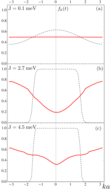
Figure 4: Solid lines: the stationary distribution functions obtained by solving discretized versions of Eqs. (17), (18) with $N_{k}=51$ momentum points and the tight-binding parameters $J$ as indicated. See text for other simulation parameters. Dashed lines: equilibrium Fermi distribution functions.

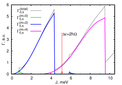
Figure 5: The transition rate (18) (arbitrary units) for scattering between the sites at $k=-\pi/a$ and $k=0$ (black, solid) and the individual contributions from $m$-photon assisted processes as indicated. The vertical dashed line at $J=5.1$ meV indicates the threshold for the $m=2$ transition, $|4\widetilde{J}|=2\hbar\Omega$; the peaks to the left and to the right of this point correspond to phonon emission and absorption, respectively.

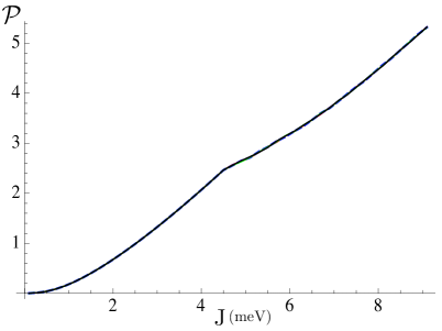
Figure 6: Scaling of the average power (arbitrary units) dissipated into the phonon modes as a function of the tight-binding parameter $J$. The four curves on top of each other correspond to the same numbers of discrete momentum points $N_{k}$ as in Fig. 3.

4 Proposed Experimental Design

The simulation results in the previous section suggest that the optimal system for third harmonic generation would be a one-dimensional metallic conductor with an unrenormalized bandwidth close to $2.6$ times the energy $\hbar\Omega$ of the driving field quanta (bandwidth of about $11$ meV for $\Omega/2\pi=1$ THz is needed), and a wide gap to reduce the absorption of the generated harmonics. One option to satisfy these requirements is to use modulated semiconductor nanowires. Here we estimate the growth parameters of an InAs/InP nanowire³⁰, which would have a near optimal band structure for generating the third harmonic of a 1 THz driving field.

We calculate the band structure of the modulated nanowire modeling it as a stack of cylinders with isotropic (bulk) electron effective masses $m^{*}_{\rm InAs}=0.073{m}_{e}$ and $m^{*}_{\rm InP}=0.027{m}_{e}$ for the InAs and InP carriers respectively, as appropriate for the nanowire diameter we used³¹. We used the barrier height of $V_{0}=0.636$ eV, found from the four-band model simulations, which is close to experimentally observed^{32, 30} $0.6$ eV. To ensure a relatively large gap, we chose the nanowire diameter $d=20$ nm, and InAs well width $w=6.0$ nm. Separating the radial and angular parts of the corresponding wave functions, we obtained a version of the Kronig-Penney model with effective mass modulation, and effective barrier dependent on the transverse momentum $\hbar\kappa_{nl}$. We plot the first few allowed energy bads as a function of InP barrier width $b$ in Fig. 7.

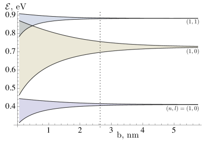
Figure 7: Energies of the three lowest bands computed using the Kronig-Penney model with effective mass modulation corresponding to an InAs/InP nanowire with diameter $d=20$ nm, InAs well width $w=6.0$ nm, plotted as a function of InP barrier width, ${b}$. The labels indicate the radial $n$ and angular $l$ quantum numbers of dimensional quantization. The dashed line at $b=2.64$ nm gives a bandwidth $10.9$ meV, or tight-binding parameter $J=2.7$, corresponding to the first maximum of the third harmonic in Fig. 3.

In particular, we conclude that an InAs/InP nanowire of diameter $d=20.0$ nm, well width of $w=6.0$ nm, and barrier width of $b=2.64$ nm [Fig. 1 (a)] would have the lowest band with a width of approximately $10.9$ meV. The next band would be separated by a gap of $280$ meV [Fig. 7]. These parameters are near optimal for third harmonic generation at $\Omega/2\pi=1$ THz.

One possible device design could involve depositing of a number of parallel modulated nanowires on a substrate, with an $s$-polarized driving field incident on the surface at angle $\theta$ so that the electric field of the wave be directed along the nanowires [Fig. 1 (b),(c)]. Then both the reflected signal and the first harmonic are going to be propagating at the same reflection angle $\theta$, while the propagation direction of the third harmonic can be found from the Snell’s law, $\sin\theta=3\sin\phi$, which accounts for the wavelengths ratio.

5 Discussion

In this work we suggest a possibility that frequency multiplication due to periodically-driven Bloch oscillation may be possible in a quasistationary setting, with the help of a narrow-band one-dimensional conductor. A quasi-equilibrium electron distribution is possible because the energy absorbed from the driving field is continuously dissipated by the bulk phonons.

For a periodically modulated InAs/InP nanowire with the period $a=8.64$ nm, and the driving field frequency $\Omega/2\pi=1$ THz, the emission of the first harmonic is suppressed with the dimensionless vector potential amplitude $A_{0}\,a\approx 3.83$, which gives the electric field amplitude $E_{0}=\hbar\Omega\,A_{0}/e\approx 1.8\times 10^{6}$ V/m, corresponding to the energy flux of about $0.5$ MWt/cm². At this kind of power, many effects could lead to eventual run-away overheating of the system, e.g., direct absorption by the substrate, or even a relatively weak disorder scattering in the nanowire. We hope that a quasi-continuous operation would still be possible, with the driving field pulse duration of a few microseconds, as opposed to few picoseconds in the experiment¹⁶.

6 Acknowledgements

The authors are grateful to Goutam Chattopadhyay, Ken Cooper, and Robert A. Suris for multiple helpful discussions, and to Craig Pryor for letting us use his dot code for nanowire calculations. This work was supported in part by the U.S. Army Research Office Grant No. W911NF-11-1-0027, and by the NSF Grant No. 1018935.

References

- Bloch 1928 Bloch, F. Z. Phys. A 1928, 52, 555–600
- Yakovlev 1961 Yakovlev, V. A. Sov. Phys.-Solid State 1961, 3, 1442, [Fiz. Tv. Tela III 1983 (1961)]
- Yakovlev 1961 Yakovlev, V. A. Sov. Phys. JETP-USSR 1961, 13, 1194, [JETP 40, 1695 (1961)]
- Keldysh 1963 Keldysh, L. V. Sov. Phys. JETP-USSR 1963, 16, 471, [JETP 43, 661 (1962)]
- Wannier 1962 Wannier, G. H. Rev. Mod. Phys. 1962, 34, 645–655
- Fukuyama et al. 1973 Fukuyama, H.; Bari, R. A.; Fogedby, H. C. Phys. Rev. B 1973, 8, 5579–5586
- Waschke et al. 1993 Waschke, C.; Roskos, H. G.; Schwedler, R.; Leo, K.; Kurz, H.; Köhler, K. Phys. Rev. Lett. 1993, 70, 3319–3322
- Mendez and Bastard 1993 Mendez, E. E.; Bastard, G. Physics Today 1993, 46, 34
- Ben Dahan et al. 1996 Ben Dahan, M.; Peik, E.; Reichel, J.; Castin, Y.; Salomon, C. Phys. Rev. Lett. 1996, 76, 4508–4511
- Pertsch et al. 1999 Pertsch, T.; Dannberg, P.; Elflein, W.; Bräuer, A.; Lederer, F. Phys. Rev. Lett. 1999, 83, 4752–4755
- Morandotti et al. 1999 Morandotti, R.; Peschel, U.; Aitchison, J. S.; Eisenberg, H. S.; Silberberg, Y. Phys. Rev. Lett. 1999, 83, 4756–9
- Christodoulides et al. 2003 Christodoulides, D. N.; Lederer, F.; Silberberg, Y. Nature 2003, 424, 817–23
- Faisal and Kamiński 1997 Faisal, F. H. M.; Kamiński, J. Z. Phys. Rev. A 1997, 56, 748–762
- Gupta et al. 2003 Gupta, A. K.; Alon, O. E.; Moiseyev, N. Phys. Rev. B 2003, 68, 205101
- Golde et al. 2008 Golde, D.; Meier, T.; Koch, S. W. Phys. Rev. B 2008, 77, 075330
- Ghimire et al. 2011 Ghimire, S.; DiChiara, A. D.; Sistrunk, E.; Agostini, P.; DiMauro, L. F.; Reis, D. A. Nature Physics 2011, 7, 138–141
- Dunlap and Kenkre 1986 Dunlap, D. H.; Kenkre, V. M. Phys. Rev. B 1986, 34, 3625–3633
- Grossmann et al. 1991 Grossmann, F.; Dittrich, T.; Jung, P.; Hänggi, P. Phys. Rev. Lett. 1991, 67, 516–519
- Keldysh 1964 Keldysh, L. V. Zh. Eksp. Teor. Fiz. 1964, 47, 1515, [Sov. Phys. JETP 20, 1018 (1965)]
- Rammer and Smith 1986 Rammer, J.; Smith, H. Rev. Mod. Phys. 1986, 58, 323–59
- Kamenev 2004 Kamenev, A. Lectures notes for 2004 Les Houches Summer School on ”Nanoscopic Quantum Transport”
- Haug and Jauho 2008 Haug, H.; Jauho, A.-P. Quantum kinetics in transport and optics of semiconductors, 2nd ed.; Springer: New York, 2008
- DeVries 1990 DeVries, P. L. J. Opt. Soc. Am. B 1990, 7, 517–520
- Joachain et al. 2011 Joachain, C. J.; Kylstra, N. J.; Potvliege, R. M. Atoms in Intense Laser Fields; Cambridge University Press: Cambridge, UK, 2011
- Kemper et al. 2013 Kemper, A. F.; Moritz, B.; Freericks, J. K.; Devereaux, T. P. New Journal of Physics 2013, 15, 023003
- Konstantinov and Perel 1960 Konstantinov, O. V.; Perel, V. I. Zh. Exp. Teor. Fiz. 1960, 39, 197–208
- Pryadko and Sengupta 2006 Pryadko, L. P.; Sengupta, P. Phys. Rev. B 2006, 73, 085321
- Hamilton et al. 2012 Hamilton, K. E.; Kovalev, A. A.; Pryadko, L. P. unpublished
- Kadanoff and Baym 1962 Kadanoff, L. P.; Baym, G. Quantum Statistical Mechanics; Benjamin: New York, 1962
- Bjork et al. 2002 Bjork, M. T.; Ohlsson, B. J.; Sass, T.; Persson, A. I.; Thelander, C.; Magnusson, M. H.; Deppert, K.; Wallenberg, L. R.; Samuelson, L. Applied Physics Letters 2002, 80, 1058–1060
- Moreira et al. 2010 Moreira, M. D.; Venezuela, P.; Miwa, R. H. Nanotechnology 2010, 21, 285204
- Thelander et al. 2004 Thelander, C.; Björk, M. T.; Larsson, M. W.; Hansen, A. E.; Wallenberg, L. R.; Samuelson, L. Solid State Communications 2004, 131, 573 – 579