Robust Adaptive Dynamic Programming for Optimal Nonlinear Control Design

Abstract

This paper studies the robust optimal control design for uncertain nonlinear systems from a perspective of robust adaptive dynamic programming (robust-ADP). The objective is to fill up a gap in the past literature of ADP where dynamic uncertainties or unmodeled dynamics are not addressed. A key strategy is to integrate tools from modern nonlinear control theory, such as the robust redesign and the backstepping techniques as well as the nonlinear small-gain theorem, with the theory of ADP. The proposed robust-ADP methodology can be viewed as a natural extension of ADP to uncertain nonlinear systems. A practical learning algorithm is developed in this paper, and has been applied to a sensorimotor control problem.

I Introduction

Reinforcement learning (RL) [30] is an important branch in machine learning theory. It is concerned with how an agent should modify its actions based on the reward from its reactive unknown environment so as to achieve a long term goal. In 1968, Werbos pointed out that the policy iteration technique devised in [6] for dynamic programming can be employed to perform RL [34]. Starting from then, many real-time RL methods for finding online optimal control policies have emerged and they are broadly called approximate/adaptive dynamic programming (ADP) [35], [36] or neurodynamic programming [5]. See [1], [2], [7], [22], [24], [31], [32], [33], for some recently developed results.

In the past literature of ADP, it is commonly assumed that the system order is known and the state variables are either fully available or reconstructible from the output; see [21], [22] and reference therein. However, in practice, the system order may be unknown due to the presence of dynamic uncertainties (or unmodeled dynamics), which are motivated by engineering applications in situations where the exact mathematical model of a physical system is not easy to be obtained. Of course, dynamic uncertainties also make sense for the mathematical modeling in other branches of science such as biology and economics. This problem, often formulated as robust control, cannot be viewed as a special case of output feedback control, and the ADP methods developed in the past literature may not only fail to guarantee optimality, but also the stability of the closed-loop system when dynamic uncertainty occurs. To fill up the above-mentioned gap in the past literature of ADP, we recently developed a new theory of robust adaptive dynamic programming (robust-ADP) [8], [10], [11], which can be viewed as a natural extension of ADP to linear and partially linear systems with dynamic uncertainties.

The primary objective of this paper is to study robust-ADP designs for genuinely nonlinear systems in the presence of dynamic uncertainties. We first decompose the open-loop system into two parts: The system model (ideal environment) with known system order and fully accessible state, and the dynamic uncertainty, with unknown system order and dynamics, interacting with the ideal environment. In order to handle the dynamic interaction between two systems, we then resort to the gain assignment idea [14], [15], [26]. More specifically, we need to assign a suitable gain for the system model with disturbance in the sense of Sontag’s input-to-state stability (ISS) [29]. The backstepping, robust redesign, and small-gain techniques in modern nonlinear control theory are incorporated into the robust-ADP theory, such that the system model is made ISS with an arbitrarily small gain. At last, the nonlinear small-gain theorem [15] is applied to analyze the stability for the interconnected systems.

Throughout this paper, vertical bars $|\!\cdot\!|$ represent the Euclidean norm for vectors, or the induced matrix norm for matrices. For any piecewise continuous function $u$, $\|u\|$ denotes ${\rm sup}\{|u(t)|,t\geq 0\}$. A function $\gamma:\mathbb{R}_{+}\rightarrow\mathbb{R}_{+}$ is said to be of class $\mathcal{K}$ if it is continuous, strictly increasing with $\gamma(0)=0$. It is of class $\mathcal{K}_{\infty}$ if additionally $\gamma(s)\rightarrow\infty$ as $s\rightarrow\infty$. A function $\beta:\mathbb{R}_{+}\times\mathbb{R}_{+}\rightarrow\mathbb{R}_{+}$ is of class $\mathcal{KL}$ if $\beta(\cdot,t)$ is of class $\mathcal{K}$ for every fixed $t\geq 0$, and $\beta(s,t)\rightarrow 0$ as $t\rightarrow\infty$ for each fixed $s\geq 0$. The notation $\gamma_{1}>\gamma_{2}$ means $\gamma_{1}(s)>\gamma_{2}(s)$, $\forall s>0$.

II Preliminaries

In this section, let us review a policy iteration technique to solve optimal control problems [27].

To begin with, consider the system

$$\dot{x}=f(x)+g(x)u$$ (1)

where $x\in\mathbb{R}^{n}$ is the system state, $u\in\mathbb{R}$ is the control input, $f,g:\mathbb{R}^{n}\rightarrow\mathbb{R}^{n}$ are locally Lipschitz functions. For any initial condition $x_{0}\in\mathbb{R}^{n}$, the cost function associated with (1) is defined as

$$J(x_{0})=\int_{0}^{\infty}\left[Q(x)+ru^{2}\right]dt,~{}~{}x(0)=x_{0}$$ (2)

where $Q(\cdot)$ is a positive definite function, and $r>0$ is a constant. In addition, assume there exists an admissible control policy $u=u_{0}(x)$ in the sense that, under this policy, the system (1) is globally asymptotically stable and the cost (2) is finite. By [20], the control policy that minimizes the cost (2) can be solved from the following Hamilton-Jacobi-Bellman (HJB) equation:

$$0=\nabla V(x)f(x)+Q(x)-\frac{1}{4r}\left[\nabla V(x)g(x)\right]^{2}$$ (3)

with the boundary condition $V(0)=0$. Indeed, if the solution $V^{*}(x)$ of (3) exists, the optimal control policy is given by

$$u^{*}(x)=-\frac{1}{2r}g(x)^{T}\nabla V^{*}(x)^{T}.$$ (4)

In general, the analytical solution of (3) is difficult to be solved. However, if $V^{*}(x)$ exists, it can be approximated using the policy iteration technique [27]:

1. Find an admissible control policy $u_{0}(x)$.

2. For any integer $i\geq 0$, solve for $V_{i}(x)$, with $V_{i}(0)=0$, using

   $$0=\nabla V_{i}(x)\left[f(x)\!+\!g(x)u_{i}(x)\right]\!+\!Q(x)\!+\!ru_{i}(x)^{2}.$$ (5)

3. Update the control policy using

   $$u_{i+1}(x)=-\frac{1}{2r}g(x)^{T}\nabla V_{i}(x)^{T}.$$ (6)

Convergence of the policy iteration (5) and (6) is concluded in the following theorem, which can be seen as a trivial extension of Theorem 4 in [27].

Theorem II.1

Consider $V_{i}(x)$ and $u_{i}(x)$ defined in (5) and (6). Then, for all $i=0,1,\cdots$,

$$V_{i+1}(x)\leq V_{i}(x),~{}~{}\forall x\in R^{n}$$ (7)

and $u_{i}(x)$ is admissible. In addition, if the solution $V^{*}(x)$ of (3) exists, then for each fixed $x$, $V_{i}(x)$ and $u_{i}(x)$ converge pointwise to $V^{*}(x)$ and $u^{*}(x)$, respectively.

III Online Learning via Robust-ADP

In this section, we develop the robust-ADP methodology for nonlinear systems as follows:

$$\dot{w} = \Delta_{w}(w,x)$$ (8)

$$\dot{x} = f(x)+g(x)\left[u+\Delta(w,x)\right]$$ (9)

where $x\in\mathbb{R}^{n}$ is the measured component of the state available for feedback control, $w\in\mathbb{R}^{p}$ is the unmeasurable part of the state with unknown order $p$, $u\in\mathbb{R}$ is the control input, $\Delta_{w}:\mathbb{R}^{p}\times\mathbb{R}^{n}\rightarrow\mathbb{R}^{p}$, $\Delta:\mathbb{R}^{p}\times\mathbb{R}^{n}\rightarrow\mathbb{R}$ are unknown locally Lipschitz functions, $f$ and $g$ are defined the same as in (1) but are assumed to be unknown.

Our design objective is to find online the control policy which stabilizes the system at the origin. Also, in the absence of the dynamic uncertainty (i.e., $\Delta=0$ and the $w$-subsystem is absent), the control policy becomes the optimal control policy that minimizes (2).

III-A Online policy iteration

The iterative technique introduced in Section 2 relies on the knowledge of $f(x)$ and $g(x)$. To remove this requirement, we develop a novel online policy iteration technique, which can be viewed as the nonlinear extension of [7].

To begin with, notice that (9) can be rewritten as

$$\dot{x} = f(x)+g(x)u_{i}(x)+g(x)v_{i}$$ (10)

where $v_{i}=u+\Delta-u_{i}$. For each $i\geq 0$, the time derivative of $V_{i}(x)$ along the solutions of (10) satisfies

$$\dot{V}_{i}(x) = -Q(x)-{r}u_{i}^{2}(x)-2ru_{i+1}(x)v_{i}.$$ (11)

Integrating both sides of (11) on any time interval $[t,t+T]$, it follows that

$$V_{i}(x(t+T))-V_{i}(x(t))$$ (12)

$$= \int_{t}^{t+T}\left[-Q(x)-ru_{i}^{2}(x)-2ru_{i+1}(x)v_{i}\right]\!dt.$$

Notice that if $u_{i}(x)$ is given, the unknown functions $V_{i}(x)$ and $u_{i+1}(x)$ can be approximated using (12). To be more specific, for any given compact set $\Omega\subset\mathbb{R}^{n}$ containing the origin as an interior point, let $\{\phi_{j}(x)\}_{j=1}^{\infty}$ be an infinite sequence of linearly independent smooth basis functions on $\Omega$, where $\phi_{j}(0)=0$ for all $j=1,2,\cdots$. Then, for each $i=0,1,\cdots$, the cost function and the control policy are approximated by $\hat{V}_{i}(x)=\sum\limits_{j=1}^{N_{1}}\hat{c}_{i,j}\phi_{j}(x)$, and $\hat{u}_{i+1}(x)=\sum\limits_{j=1}^{N_{2}}\hat{w}_{i,j}\phi_{j}(x)$, respectively, where $N_{1}>0$, $N_{2}>0$ are two sufficiently large integers, and $\hat{c}_{i,j}$, $\hat{w}_{i,j}$ are constant weights to be determined.

Replacing $V_{i}(x)$, $u_{i}(x)$, and $u_{i+1}(x)$ in (12) with their approximations, we obtain

$$\sum\limits_{j=1}^{N_{1}}\hat{c}_{i,j}\left[\phi_{j}(x(t_{k+1}))-\phi_{j}(x(t_{k}))\right]$$

$$= -\int_{t_{k}}^{t_{k+1}}2r\sum\limits_{j=1}^{N_{2}}\hat{w}_{i,j}\phi_{j}(x)\hat{v}_{i}dt$$

$$-\int_{t_{k}}^{t_{k+1}}\left[Q(x)+r\hat{u}_{i}^{2}(x)\right]dt+e_{i,k}$$

where $\hat{u}_{0}=u_{0}$, $\hat{v}_{i}=u+\Delta-\hat{u}_{i}$, and $\{t_{k}\}_{k=0}^{l}$ is a strictly increasing sequence with $l>0$ a sufficiently large integer. Then, the weights $\hat{c}_{i,j}$ and $\hat{w}_{i,j}$ can be solved in the sense of least-squares (i.e., by minimizing $\sum_{k=0}^{l}e_{i,k}^{2}$).

Now, starting from $u_{0}(x)$, two sequences $\{\hat{V}_{i}(x)\}_{i=0}^{\infty}$, and $\{\hat{u}_{i+1}(x)\}^{\infty}_{i=0}$ can be generated via the online policy iteration technique (III-A). Next, we show the convergence of the sequences to $V_{i}(x)$ and $u_{i+1}(x)$, respectively.

Assumption III.1

There exist $l_{0}>0$ and $\delta>0$, such that for all $l\geq l_{0}$, we have

$$\frac{1}{l}\sum\limits_{k=0}^{l}\theta_{i,k}^{T}\theta_{i,k}\geq\delta I_{N_{1}+N_{2}}$$ (14)

where

$$\theta_{i,k}^{T}=\left[\begin{array}[]{c}\phi_{1}(x({t_{k+1}}))-\phi_{1}(x(t_{k}))\\ \phi_{2}(x({t_{k+1}}))-\phi_{2}(x(t_{k}))\\ \vdots\\ \phi_{N_{1}}(x({t_{k+1}}))-\phi_{N_{1}}(x(t_{k}))\\ 2r\int_{t_{k}}^{t_{k+1}}\phi_{1}(x)\hat{v}_{i}(x)dt\\ 2r\int_{t_{k}}^{t_{k+1}}\phi_{2}(x)\hat{v}_{i}(x)dt\\ \vdots\\ 2r\int_{t_{k}}^{t_{k+1}}\phi_{N_{2}}(x)\hat{v}_{i}(x)dt\end{array}\right]\in\mathbb{R}^{N_{1}+N_{2}}.$$

Assumption III.2

For all $t\geq 0$, we have $x(t)\in\Omega$.

Notice that, Assumption III.2 is not very restrictive and can be satisfied if $\Omega$ is an invariant set for the $x$-subsystem. This issue will be further elaborated in Section V.

Theorem III.1

Under Assumptions III.1 and III.2, for each $i\geq 0$, we have

$$\lim_{N_{1},N_{2}\rightarrow\infty}\hat{V}_{i}(x)~{}~{} = {V}_{i}(x),$$ (16)

$$\lim_{N_{1},N_{2}\rightarrow\infty}\hat{u}_{i+1}(x) = {u}_{i+1}(x),$$ (17)

for all $x\in\Omega.$

Proof:

See the Appendix. ∎

Corollary III.1

Under Assumptions III.1 and III.2, for any arbitrary $\epsilon>0$, there exist integers $i^{*}>0$, $N_{1}^{*}>0$ and $N^{*}_{2}>0$, such that

$$|\hat{V}_{i}(x)-V^{*}(x)|\leq\epsilon,~{}~{}{\rm and}~{}~{}|\hat{u}_{i+1}(x)-u^{*}(x)|\leq\epsilon,$$

for all $x\in\Omega$, if $i>i^{*}$, $N_{1}>N_{1}^{*}$, and $N_{2}>N_{2}^{*}$.

III-B Robust redesign

In the presence of the dynamic uncertainty, we redesign the approximated optimal control policy so as to achieve asymptotic stability. This method is an integration of optimal control theory [20] with the gain assignment technique [15], [26]. To begin with, let us assume the following:

Assumption III.3

There exists a function ${\underline{\alpha}}$ of class $\mathcal{K}_{\infty}$, such that for $i=0,1,\cdots$,

$${\underline{\alpha}}(|x|)\leq V_{i}(x),~{}~{}\forall x\in\mathbb{R}^{n}.$$ (18)

In addition, assume there exists a constant $\epsilon>0$ such that $Q(x)-\epsilon^{2}|x|^{2}$ is a positive definite function.

Notice that, we can also find a class $\mathcal{K}_{\infty}$ function ${\bar{\alpha}}$, such that for $i=0,1,\cdots$,

$$V_{i}(x)\leq{\bar{\alpha}}(|x|),~{}~{}\forall x\in\mathbb{R}^{n}.$$ (19)

Assumption III.4

Consider (8). There exist functions ${\underline{\lambda}},{\bar{\lambda}}\in\mathcal{K}_{\infty}$, $\kappa_{1},\kappa_{2},\kappa_{3}\in\mathcal{K}$, and positive definite functions $W$ and $\kappa_{4}$, such that for all $w\in\mathbb{R}^{p}$ and $x\in\mathbb{R}^{n}$, we have

$${{\underline{\lambda}}}(|w|)\leq W(w)\leq{{\bar{\lambda}}}(|w|),$$ (20)

$$|\Delta(w,x)|\leq\max\{\kappa_{1}(|w|),\kappa_{2}(|x|)\},$$ (21)

together with the following implication:

$$W(w)\geq\kappa_{3}(|x|)\Rightarrow\nabla W(w)\Delta_{w}(w,x)\leq-\kappa_{4}(w).$$ (22)

Assumption III.4 implies that the $w$-system (8) is input-to-state stable (ISS) [29] when $x$ is considered as the input, i.e.,

$$|w(t)|\leq\beta_{w}(|w(0)|,t)+\gamma_{w}(\|x\|)$$ (23)

where $\beta_{w}$ is of class $\mathcal{KL}$ and $\gamma_{w}$ is of class $\mathcal{K}$.

Now, consider the following type of control policy

$$u_{ro}(x)=\left[1+\frac{r}{2}\rho^{2}(|x|^{2})\right]\hat{u}_{i^{*}+1}(x)$$ (24)

where $i^{*}>0$ is a sufficiently large integer as defined in Corollary III.1, $\rho$ is a smooth, non decreasing function, with $\rho(s)>0$ for all $s\geq 0$. Notice that $u_{ro}$ can be viewed as a robust redesign of the approximated optimal control law $\hat{u}_{i^{*}+1}$.

As in [14], let us define a class $\mathcal{K}_{\infty}$ function $\gamma$ by

$$\gamma(s)=\frac{1}{2}\epsilon\rho(s^{2})s,~{}~{}\forall s\geq 0.$$ (25)

In addition, define

$$e_{ro}(x) = \frac{r}{2}\rho^{2}(|x|^{2})\left[\hat{u}_{i^{*}+1}(x)-{u}_{i^{*}+1}(x)\right]$$ (26)

$$+\hat{u}_{i^{*}+1}(x)-u_{i^{*}}(x).$$

Theorem III.2

Under Assumptions III.3 and III.4, suppose

$${\gamma}>\max\{\kappa_{2},\kappa_{1}\circ{\underline{\lambda}}^{-1}\circ\kappa_{3}\circ{\underline{\alpha}}^{-1}\circ{\bar{\alpha}}\},$$ (27)

and the following implication holds for some constant $d>0$:

$$0<V_{i^{*}}(x)\leq d\Rightarrow|e_{ro}(x)|<{\gamma}(|x|).$$ (28)

Then, the closed-loop system composed of (8), (9), and (24) is asymptotically stable at the origin. In addition, there exists $\sigma\in\mathcal{K}_{\infty}$, such that $\Omega_{i^{*}}=\{(w,x):\max\left[\sigma(V_{i^{*}}(x)),W(w)\right]\leq\sigma(d)\}$ is an estimate of the region of attraction of the closed-loop system.

Proof:

See the Appendix. ∎

Remark III.1

In the absence of the dynamic uncertainty (i.e., $\Delta=0$ and the $w$-system is absent), the control policy (24) can be replaced by $\hat{u}_{i^{*}+1}(x)$, which is an approximation of the optimal control policy $u^{*}(x)$ that minimizes the following cost function

$$J(x_{0})=\int_{0}^{\infty}\left[Q(x)+{r}u^{2}\right]dt,~{}~{}x(0)=x_{0}.$$ (29)

IV Robust-ADP with unmatched dynamic uncertainty

In this section, we extend the robust-ADP methodology to nonlinear systems with unmatched dynamic uncertainties. To begin with, consider the system:

$$\dot{w} = \Delta_{w}(w,x)$$ (30)

$$\dot{x} = f(x)+g(x)\left[z+\Delta(w,x)\right]$$ (31)

$$\dot{z} = f_{1}(x,z)+u+\Delta_{1}(w,x,z)$$ (32)

where $[x^{T},z]^{T}\in\mathbb{R}^{n}\times\mathbb{R}$ is the measured component of the state available for feedback control; $w$, $u$, $\Delta_{w}$, $f$, $g$, and $\Delta$ are defined in the same way as in (8)-(9); $f_{1}:\mathbb{R}^{n}\times\mathbb{R}\rightarrow\mathbb{R}$ and $\Delta_{1}:\mathbb{R}^{p}\times\mathbb{R}^{n}\times\mathbb{R}\rightarrow\mathbb{R}$ are locally Lipschitz functions and are assumed to be unknown.

Assumption IV.1

There exist class $\mathcal{K}$ functions $\kappa_{5},\kappa_{6},\kappa_{7}$, such that the following inequality holds:

$$|\Delta_{1}(w,x,z)|\leq\max\{\kappa_{5}\left(|w|\right),\kappa_{6}\left(|x|\right),\kappa_{7}\left(|z|\right)\}.$$ (33)

IV-A Online learning

Let us define a virtual control policy $\xi=u_{ro}$, as defined in (24). Then, a state transformation can be performed as $\zeta=z-\xi$. Along the trajectories of (31)-(32), it follows that

$$\dot{\zeta}=\bar{f}_{1}(x,z)+u+\Delta_{1}-\bar{g}_{1}(x)\Delta$$ (34)

where $\bar{f}_{1}(x,z)=f_{1}(x,z)-\frac{\partial\xi}{\partial x}f(x)-\frac{\partial\xi}{\partial x}g(x)z$, and $\bar{g}_{1}(x)=\frac{\partial\xi}{\partial x}g(x)$ are two unknown functions that can be approximated by $\hat{f}_{1}(x,z)=\sum_{j=1}^{N_{3}}\hat{w}_{f,j}\psi_{j}(x,z)$ and $\hat{g}_{1}(x)=\sum_{j=0}^{N_{4}-1}\hat{w}_{g,j}\phi_{j}(x)$, respectively, where $\{\psi_{j}(x,z)\}_{j=1}^{\infty}$ is a sequence of linearly independent basis functions on some compact set $\Omega_{1}\in\mathbb{R}^{n+1}$ containing the origin as its interior, $\phi_{0}(x)\equiv 1$, $\hat{w}_{f,j}$ and $\hat{w}_{g,j}$ are constant weights to be trained. As in the matched case, $\Omega_{1}$ is selected to be an invariant set for the system (31) and (32).

IV-A1 Phase-one learning

To approximate the virtual control input $\xi$ for the $x$-subsystem, the same procedure as in (III-A) can be applied, with $\hat{v}_{i}=z+\Delta-\hat{u}_{i}$.

IV-A2 Phase two learning

To approximate the unknown functions $\bar{f}_{1}$ and $\bar{g}_{1}$, The constant weights can be solved, in the sense of least-squares, from

$$\frac{1}{2}\zeta^{2}(t_{k+1}^{\prime})-\frac{1}{2}\zeta^{2}(t_{k}^{\prime})$$ (35)

$$= \int_{t_{k}^{\prime}}^{t_{k+1}^{\prime}}\left[\sum_{j=1}^{N_{3}}\hat{w}_{f,j}\psi_{j}(x,z)-\sum_{j=0}^{N_{4}-1}\hat{w}_{g,j}\phi_{j}(x)\Delta\right]\zeta dt$$

$$+\int_{t_{k}^{\prime}}^{t_{k+1}^{\prime}}(u+\Delta_{1})\zeta dt+\bar{e}_{k}$$

where $\{t_{k}^{\prime}\}_{k=1}^{l}$ is a strictly increasing positive constant sequence with $l>0$ a sufficiently large integer, and $\bar{e}_{k}$ denotes the approximation error. Similarly as in the previous section, let us introduce the following assumption:

Assumption IV.2

There exist $l_{1}>0$ and $\delta_{1}>0$, such that for all $l\geq l_{1}$, we have

$$\frac{1}{l}\sum\limits_{k=0}^{l}\bar{\theta}_{k}^{T}\bar{\theta}_{k}\geq\delta_{1}I_{N_{3}+N_{4}}$$ (36)

where

$$\bar{\theta}_{k}^{T}=\left[\begin{array}[]{c}\int_{t_{k}^{\prime}}^{t_{k+1}^{\prime}}\psi_{1}(x,z)\zeta dt\\ \int_{t_{k}^{\prime}}^{t_{k+1}^{\prime}}\psi_{2}(x,z)\zeta dt\\ \vdots\\ \int_{t_{k}^{\prime}}^{t_{k+1}^{\prime}}\psi_{N_{3}}(x,z)\zeta dt\\ \int_{t_{k}^{\prime}}^{t_{k+1}^{\prime}}\phi_{0}(x)\Delta\zeta dt\\ \int_{t_{k}^{\prime}}^{t_{k+1}^{\prime}}\phi_{1}(x)\Delta\zeta dt\\ \vdots\\ \int_{t_{k}^{\prime}}^{t_{k+1}^{\prime}}\phi_{N_{4}-1}(x)\Delta\zeta dt\end{array}\right]\in\mathbb{R}^{N_{3}+N_{4}}.$$

Theorem IV.1

Consider $(x(0),z(0))\in\Omega_{1}$. Then, under Assumption IV.2 we have

$$\lim_{N_{3},N_{4}\rightarrow\infty}\hat{f}(x,z) = \bar{f}_{1}(x,z),$$ (38)

$$\lim_{N_{3},N_{4}\rightarrow\infty}\hat{g}(x)~{}~{}~{} = \bar{g}_{1}(x),~{}~{}\forall(x,z)\in\Omega_{1}.$$ (39)

Theorem IV.1 can be proved following the same idea as in the proof of Theorem 3.1, and is omitted here for want of space.

IV-B Robust redesign

Next, we study robust stabilization of the system (30)-(32). To this end, let $\kappa_{8}$ be a function of $\mathcal{K}$ such that

$$\kappa_{8}(|x|)\geq|\xi(x)|,~{}~{}\forall x\in\mathbb{R}^{n}.$$ (40)

Then, Assumption IV.1 implies

$$|\Delta_{1}| \leq \max\{\kappa_{5}\left(|w|\right),\kappa_{6}\left(|x|\right),\kappa_{7}\left(|z|\right)\}$$

$$\leq \max\{\kappa_{5}\left(|w|\right),\kappa_{6}\left(|x|\right),\kappa_{7}\left(|\xi|+\kappa_{8}(|x|)\right)\}$$

$$\leq \max\{\kappa_{5}\left(|w|\right),\kappa_{9}\left(|X_{1}|\right)\}$$

where $\kappa_{9}(s)=\max\{\kappa_{6},\kappa_{7}\circ\kappa_{8}\circ(2s),\kappa_{7}\circ(2s)\}$, $\forall s\geq 0$. In addition, we denote $\tilde{\kappa}_{1}=\max\{\kappa_{1},\kappa_{5}\}$, $\tilde{\kappa}_{2}=\max\{\kappa_{2},\kappa_{9}\}$, $\gamma_{1}(s)=\frac{1}{2}\epsilon\rho(\frac{1}{2}s^{2})s$, and

$$U_{i^{*}}(X_{1})=V_{i^{*}}(x)+\frac{1}{2}\zeta^{2}.$$ (41)

Notice that, under Assumptions III.3 and III.4, there exist $\bar{\alpha}_{1},\underline{\alpha}_{1}\in\mathcal{K}_{\infty}$, such that $\underline{\alpha}_{1}(|X_{1}|)\leq U_{i^{*}}(X_{1})\leq\bar{\alpha}_{1}(|X_{1}|)$.

The control policy can be approximated by

$$\!\!{u}_{ro1}\!\! \!\!=\!\! \!\!-\hat{f}_{1}(x,z)+2r\hat{u}_{i^{*}+1}(x)$$

$$-\frac{\hat{g}^{2}(x)\rho_{1}^{2}(|X_{1}|^{2})\zeta}{4}-\epsilon^{2}\zeta$$

$$-\frac{\rho_{1}^{2}(|X_{1}|^{2})\zeta}{4}-\frac{\epsilon^{2}\rho^{2}(\zeta^{2})\zeta}{2\rho^{2}(|x|^{2})}$$

where ${X}_{1}=[x^{T},\zeta]^{T}$, and $\rho_{1}(s)=2\rho(\frac{1}{2}s)$.

Next, define the approximation error as

$$\!\!e_{ro1}(X_{1})\!\! \!\!=\!\! \!\!-\bar{f}_{1}(x,z)+\hat{f}_{1}(x,z)$$ (43)

$$+2r\left[{u}_{i^{*}+1}(x)-\hat{u}_{i^{*}+1}(x)\right]$$

$$-\frac{\left[\bar{g}_{1}^{2}(x)-\hat{g}_{1}^{2}(x)\right]\rho_{1}^{2}(|X_{1}|^{2})\zeta}{4}$$

Then, conditions for asymptotic stability are summarized in the following Theorem:

Theorem IV.2

Under Assumptions III.3, III.4, and IV.1, if

$$\gamma_{1}>\max\{\tilde{\kappa}_{2},\tilde{\kappa}_{1}\circ\underline{\lambda}^{-1}\circ\kappa_{3}\circ\underline{\alpha}_{1}^{-1}\circ\bar{\alpha}_{1}\},$$ (44)

and if the following implication holds for some constant $d_{1}>0$:

$$0<U_{i^{*}}(X_{1})\leq d_{1}\Rightarrow\max\{|e_{ro1}(X_{1})|,|e_{ro}(x)|\}<{\gamma}_{1}(|X_{1}|),$$

then the closed-loop system comprised of (30)-(32), and (IV-B) is asymptotically stable at the origin. In addition, there exists $\sigma_{1}\in\mathcal{K}_{\infty}$, such that

$${\Omega}_{1,i^{*}}=\{(w,X_{1}):\max\left[\sigma_{1}(U_{i^{*}}(X_{1})),W(w)\right]\leq\sigma_{1}(d_{1})\}$$

is an estimate of the region of attraction.

Proof:

See the Appendix. ∎

Remark IV.1

In the absence of the dynamic uncertainty (i.e., $\Delta=0$, $\Delta_{1}=0$ and the $w$-system is absent), the smooth functions $\rho$ and $\rho_{1}$ can all be replaced by $0$, and the system dynamics becomes

$$\dot{X}_{1}=F_{1}(X_{1})+G_{1}u_{o1}$$ (45)

where $F_{1}(X_{1})=\left[\begin{array}[]{c}f(x)+g(x)\zeta+g(x)\xi\\ -\nabla V_{i^{*}}(x)g(x)\end{array}\right]$, $G_{1}=\left[\begin{array}[]{c}0\\ 1\end{array}\right]$, and $u_{o1}=-\epsilon^{2}\zeta^{2}$. As a result, it can be concluded that the control policy $u=u_{o1}$ is an approximate optimal control policy with respect to the cost function

$$J_{1}(X_{1}(0))=\int_{0}^{\infty}\left[Q_{1}\left(x,\zeta\right)+\frac{1}{2\epsilon^{2}}u^{2}\right]dt$$ (46)

with $X_{1}(0)=[x_{0}^{T},z_{0}-u_{i^{*}}(x_{0})]^{T}$ and $Q_{1}\left(x,\zeta\right)=Q\left(x\right)+\frac{1}{4r}\left[\nabla V_{i^{*}}(x)g(x)\right]^{2}+\frac{\epsilon^{2}}{2}\zeta^{2}.$

V Implementation Issues

In this section, we study a few implementation issues on the robust-ADP based online learning methodology, and give a practical algorithm. Due to the space limitation, we will mainly focus on the systems with matched dynamic uncertainties. These results can be easily extended to the unmatched case.

V-A The compact set for approximation

Assumption V.1

The closed-loop system composed of (8), (9), and

$$u=u_{0}(x)+e$$ (47)

is ISS when $e$, the exploration noise, is considered to be the input.

The reason for imposing Assumption V.1 is two fold. First, like in many other policy iteration based ADP algorithms, an initial admissible control policy is desired. In this paper we further assume the initial control policy is stabilizing in the presence of dynamic uncertainties. Such an assumption is feasible and realistic by means of the designs in [14], [26]. Second, by adding the exploration noise, we are able to satisfy Assumptions III.1 and IV.2, and at the same time keep the system solutions bounded.

Under Assumption V.1, we can find a compact set $\Omega_{0}$ which is an invariant set of the closed-loop system compose of (8), (9), and $u=u_{0}(x)$. In addition, we can also let $\Omega_{0}$ contain $\Omega_{i^{*}}$ as its subset. Then, the compact set for approximation can be selected as $\Omega=\{x|\exists w,{\rm~{}s.t.}~{}(x,w)\in\Omega_{0}\}$.

V-B Two-loop optimization scheme

In general cases, it may be difficult to determine the number of basis functions to be used for approximation. In this paper we propose a two-loop online optimization scheme as shown in Fig. 1. In the inner loop, least-squares method is used to train the weights. If the residual sum of errors is greater than a given threshold $\bar{\epsilon}>0$, in the outer loop the number of basis functions are increased and online data are recollected to solve the minimization problem until sufficient small residual error can be obtained.

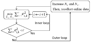
Figure 1: Two-loop online optimization scheme

V-C Robust-ADP algorithm

The robust-ADP algorithm is given in Algorithm 1.

1. Let $(w(0),x(0))\in\Omega_{i^{*}}$, employ the initial control policy (47) and collect the system state and input information.

2. Apply the online policy iteration using (III-A), and redesign the control policy using (24).

3. Terminate the exploration noise $e$.

4. If $(w(t),x(t))\in\Omega_{i^{*}}$, apply the approximate robust optimal control policy (24).

Algorithm 1 Robust-ADP Algorithm

VI Application to a single-joint human arm movement control problem

In this section, we apply the proposed online learning strategy to study a sensorimotor control problem. A linear version of this problem has been studied in [12].

Consider a single-joint arm movement as shown in Fig. 2, where the position of the elbow is fixed. The dynamic model is shown below [28].

$$I\ddot{\theta}=-mgl\cos(\theta)+n+T_{m}$$ (48)

where $m$ is the mass of segment, $I$ is the inertia, $g$ is the gravitational constant, $l$ is the distance of the center of mass from the joint, $\theta$ is the joint angular position, $T_{m}$ is the input to the muscle from the motorneurons, and $n$ denotes the inputs from the neural integrator, which can be modeled by a low pass filter as follows with a time constant $\tau_{N}$.

$$\dot{n}=-\frac{n}{\tau_{N}}+T_{m}.$$ (49)

Let us define $x_{1}=\theta-\theta_{0}$, $x_{2}=\dot{\theta}$, $w=n-\frac{\tau_{N}mgl\cos(\theta_{0})}{\tau_{N}+1}-Ix_{2}$, $u=T_{m}-\frac{mgl\cos(\theta_{0})}{\tau_{N}+1}$, where $\theta_{0}$ is the desired end point angular position. Then, the system can be converted to

$$\dot{w}_{~{}} = -\frac{1+\tau_{N}}{\tau_{N}}(w+Ix_{2})$$ (51)

$$-{2mgl}\sin(\frac{x_{1}}{2})\sin(\frac{x_{1}}{2}+\theta_{0})$$

$$\dot{x}_{1} = x_{2}$$ (52)

$$\dot{x}_{2} = \frac{2mgl}{I}\sin(\frac{x_{1}}{2})\sin(\frac{x_{1}}{2}+\theta_{0})$$

$$+\frac{1}{I}\left(u+Ix_{2}+w\right)$$

To apply the proposed robust-ADP method, the basis functions we used are polynomials with degrees less than or equal to five. The invariant set is chosen to contain the region $\{(w,x_{1},x_{2}):|w|\leq 1,|x_{1}|\leq 0.8,|x_{2}|\leq 3.5\}$. Only for simulation purpose, we set $\theta_{0}=\frac{\pi}{4}$, $m=1.65$, $l=0.179$, $g=9.81$, $I=0.0779$. An initial control policy is set to be $u_{0}=-0.5x_{1}-0.5x_{2}$. The initial condition is set to be $w(0)=1$, $x_{1}(0)=-\frac{\pi}{4}$, and $x_{2}(0)=0$. The optimal cost is specified as $J=\int_{0}^{\infty}\left(100x_{1}^{2}+x_{2}^{2}+u^{2}\right)dt$.

In this simulation, the convergence is attained after $10$ iterations. It can be seen from Fig. 3 that the approximated cost function $\hat{V}_{10}(x)$ is remarkably reduced compared with the initial approximated cost $\hat{V}_{0}(x)$. Also, in Fig. 4, we compare the speed curves under the initial control policy, the policy after two iterations, and the policy after 10 iterations. Clearly, after enough iteration steps, the speed profile becomes a bell-shaped curve which is consistent with experimental observations (see, for example, [3]).

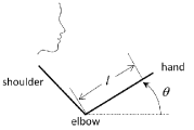
Figure 2: Single-joint arm movement control problem.

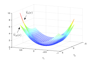
Figure 3: Comparison of the approximated cost functions.

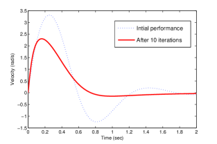
Figure 4: Comparison of the speed profiles.

VII Conclusions

In this paper, computational robust optimal controller design has been studied for nonlinear systems with dynamic uncertainties. Both the matched and the unmatched cases are studied. We have presented for the first time a recursive, online, adaptive optimal controller design when dynamic uncertainties, characterized by input-to-state stable systems with unknown order and states/dynamics, are taken into consideration. We have achieved this goal by integration of approximate/adaptive dynamic programming (ADP) theory and several tools recently developed within the nonlinear control community. Systematic robust-ADP based online learning algorithm has been developed. Rigorous stability analysis based on Lyapunov and small-gain techniques is carried out. The effectiveness of the proposed methodology has been validated by its application to a single-joint arm movement control problem.

Proof of Theorem 3.1

To begin with, given $\hat{u}_{i}$, let $\tilde{V}_{i}(x)$ be the solution of the following equation with $\tilde{V}_{i}(0)=0$.

$$\nabla{\tilde{V}_{i}}(x)\left(f(x)+g(x)\hat{u}_{i}(x)\right)+Q(x)+r\hat{u}_{i}^{2}(x)=0$$ (54)

and denote $\displaystyle\tilde{u}_{i+1}(x)=-\frac{1}{2r}g(x)^{T}\nabla\tilde{V}_{i}(x)^{T}$.

Lemma .1

For each $i\geq 0$, we have $\lim\limits_{N_{1},N_{2}\rightarrow\infty}\hat{V}_{i}(x)=\tilde{V}_{i}(x)$, $\lim\limits_{N_{1},N_{2}\rightarrow\infty}\hat{u}_{i+1}(x)=\tilde{u}_{i+1}(x)$, $\forall x\in\Omega$.

Proof:

By definition

$$\tilde{V}_{i}(x(t_{k+1}))-\tilde{V}_{i}(x(t_{k}))$$ (55)

$$= -\int_{t_{k}}^{t_{k+1}}[Q(x)+r\hat{u}_{i}^{2}(x)+2r\tilde{u}_{i+1}(x)\hat{v}_{i}(x)]dt$$

Let $\tilde{c}_{i,j}$ and $\tilde{w}_{i,j}$ be the constant weights such that $\tilde{V}_{i}(x)=\sum_{j=1}^{\infty}\tilde{c}_{i,j}\phi_{j}(x)$ and $\tilde{u}_{i+1}(x)=\sum_{j=1}^{\infty}\tilde{w}_{i,j}\phi_{j}(x)$. Then, by (III-A) and (55), we have $e_{i,k}=\theta_{i,k}^{T}\bar{W}_{i}+\xi_{i,k}$, where

$$\bar{W_{i}}\! \!=\! \!~{}~{}\left[\begin{array}[]{cccccccc}\!\tilde{c}_{i,1}\!&\!\tilde{c}_{i,2}\!&\!\cdots\!&\!\tilde{c}_{i,N_{{}_{1}}}\!&\!\tilde{w}_{i,1}\!&\!\tilde{w}_{i,2}\!&\!\cdots\!&\!\tilde{w}_{i,N_{{}_{2}}}\end{array}\right]^{T}$$

$$\!-\left[\begin{array}[]{cccccccc}\hat{c}_{i,1}\!&\!\hat{c}_{i,2}\!&\!\cdots\!&\!\hat{c}_{i,N_{{}_{1}}}\!&\!\hat{w}_{i,1}\!&\!\hat{w}_{i,2}\!&\!\cdots\!&\!\hat{w}_{i,N_{{}_{2}}}\end{array}\right]^{T},$$

$$\xi_{i,k}\!\! \!\!=\! \!\sum_{j=N_{1}+1}^{\infty}\tilde{c}_{i,j}\left[\phi_{j}(x(t_{k+1}))-\phi_{j}(x(t_{k}))\right]$$

$$+\sum_{j=N_{2}+1}^{\infty}\tilde{w}_{i,j}\int_{t_{k}}^{t_{k+1}}2r\phi_{j}(x)\hat{v}_{i}dt.$$

Since the weights are found using the least-squares method, we have

$$\sum_{k=1}^{l}e_{i,k}^{2}\leq\sum_{k=1}^{l}\xi_{i,k}^{2}$$

Also notice that,

$$\sum\limits_{k=1}^{l}\bar{W}_{i}^{T}\theta_{i,k}^{T}\theta_{i,k}\bar{W_{i}}=\sum\limits_{k=1}^{l}(e_{i,k}-\xi_{i,k})^{2}$$

Then, under Assumption III.1, it follows that

$$\bar{|W_{i}|}^{2}\leq\frac{4|\Xi_{i,l}|^{2}}{l\delta}=\frac{4}{\delta}\max_{1\leq k\leq l}\xi_{i,k}^{2}.$$

Therefore, given any arbitrary $\epsilon>0$, we can find $N_{10}>0$ and $N_{20}>0$, such that when $N_{1}>N_{10}$ and $N_{2}>N_{20}$, we have

$$|\hat{V}_{i}(x)-\tilde{V}_{i}(x)|$$ (58)

$$\leq \sum_{j=1}^{N_{1}}|c_{i,j}-\hat{c}_{i,j}||\phi_{j}(x)|+\sum_{j=N_{1}+1}^{\infty}|c_{i,j}\phi_{j}(x)|$$ (59)

$$\leq \frac{\epsilon}{2}+\frac{\epsilon}{2}=\epsilon,~{}~{}\forall x\in\Omega.$$ (60)

Similarly, $|\hat{u}_{i+1}(x)-\tilde{u}_{i+1}(x)|\leq\epsilon$. The proof is complete. ∎

We now prove Theorem 3.1 by induction:

1) If $i=0$ we have $\tilde{V_{0}}(x)=V_{0}(x)$, and $\tilde{u}_{1}(x)=u_{1}(x)$. Hence, the convergence can directly be proved by Lemma A.1.

2) Suppose for some $i>0$, we have $\lim_{N_{1},N_{2}\rightarrow\infty}\hat{V}_{i-1}(x)={V}_{i-1}(x)$, $\lim_{N_{1},N_{2}\rightarrow\infty}\hat{u}_{i}(x)={u}_{i}(x)$, $\forall x\in\Omega$. By definition, we have

$$|V_{i}(x(t))-\tilde{V}_{i}(x(t))|$$

$$= r|\int_{t}^{\infty}\left[\hat{u}_{i}(x)^{2}-u_{i}(x)^{2}\right]dt|$$

$$+ 2r|\int_{t}^{\infty}u_{i+1}(x)g(x)\left[\hat{u}_{i}(x)-u_{i}(x)\right]dt|$$

$$+ 2r|\int_{t}^{\infty}\left[\hat{u}_{i+1}(x)-u_{i+1}(x)\right]g(x)\hat{v}_{i}dt|,~{}~{}\forall x\in\Omega.$$

By the induction assumptions, we known

$$\lim\limits_{N_{1},N_{2}\rightarrow\infty}\int_{t}^{\infty}\left[\hat{u}_{i}(x)^{2}-u_{i}(x)^{2}\right]dt=0$$ (61)

$$\lim\limits_{N_{1},N_{2}\rightarrow\infty}\int_{t}^{\infty}u_{i+1}(x)g(x)\left[\hat{u}_{i}(x)-u_{i}(x)\right]dt=0$$ (62)

Also, by Assumption III.1, we conclude

$$\lim\limits_{N_{1},N_{2}\rightarrow\infty}|{u}_{i+1}(x)-\hat{u}_{i+1}(x)|=0$$ (63)

and

$$\lim\limits_{N_{1},N_{2}\rightarrow\infty}|{V}_{i}(x)-\tilde{V}_{i}(x)|=0.$$ (64)

Finally, since

$$|\hat{V}_{i}(x)-V_{i}(x)|\leq|V_{i}(x)-\tilde{V}_{i}(x)|+|\tilde{V}_{i}(x)-\hat{V}_{i}(x)|$$

and by the induction assumption, we have

$$\lim\limits_{N_{1},N_{2}\rightarrow\infty}|{V}_{i}(x)-\hat{V}_{i}(x)|=0.$$ (65)

The proof is thus complete.

Proof of Theorem 3.2

Define

$$\bar{e}_{ro}(x)=\left\{\begin{array}[]{cc}e_{ro}(x),&V_{i^{*}}(x)\leq d\\ 0,&V_{i^{*}}(x)>d\end{array}\right.$$ (68)

and

$$u(x)=u_{i^{*}}(x)+\frac{r}{2}\rho^{2}(|x|^{2}){u}_{i^{*}+1}(x)+\bar{e}_{ro}(x)$$ (69)

Then, along the solutions of (9), by completing the squares, we have

$$\dot{V}_{i^{*}}(x)$$

$$\leq -Q(x)+\frac{1}{\rho^{2}(|x|^{2})}(\Delta+\bar{e}_{ro}(x))^{2}$$

$$= -(Q(x)-\epsilon^{2}|x|^{2})-\frac{4\gamma^{2}-(\Delta+\bar{e}_{ro}(x))^{2}}{\rho^{2}(|x|^{2})}$$

$$\leq -Q_{0}(x)-4\frac{\gamma^{2}-\max\{\kappa^{2}_{1}(|w|),\kappa^{2}_{2}(|x|),\bar{e}_{ro}^{2}(|x|)\}}{\rho^{2}(|x|^{2})}$$

where $Q_{0}(x)=Q(x)-\epsilon^{2}|x|^{2}$ is a positive definite function of $x$.

Therefore, under Assumptions III.3, III.4 and the gain condition (27), we have the following implication:

$$\!\!V_{i^{*}}(x)\geq{\bar{\alpha}}\!\circ\!\gamma^{-1}\!\circ\!\kappa_{1}\!\circ\!{\underline{\lambda}}^{-1}\!\left(W(w)\right)$$

$$\!\!\Rightarrow\!\! \!\!|x|\geq\gamma^{-1}\circ\kappa_{1}\circ{\underline{\lambda}}^{-1}\left(W(w)\right)$$

$$\!\!\Rightarrow\!\! \!\!\gamma\left(|x|\right)\geq\kappa_{1}\left(|w|\right)$$

$$\!\!\Rightarrow\!\! \!\!\gamma\left(|x|\right)\geq\max\{\kappa_{1}\left(|w|\right),\kappa_{2}\left(|x|\right),\bar{e}_{ro}\left(|x|\right)\}$$

$$\!\!\Rightarrow\!\! \!\!\dot{V}_{i^{*}}(x)\leq-Q_{0}(x).$$

Also, under Assumption III.4, we have

$$W(w)\geq\kappa_{3}\circ{{\underline{\alpha}}^{-1}(V_{i^{*}}(x))}$$ (71)

$$\Rightarrow W(w)\geq\kappa_{3}(|x|)$$

$$\Rightarrow \nabla W(w)\Delta_{w}(w,x)\leq-\kappa_{4}(|w|).$$

Finally, under the gain condition (27), it follows that

$${\gamma}(s)>\kappa_{1}\circ{\underline{\lambda}}^{-1}\circ\kappa_{3}\circ{\underline{\alpha}}^{-1}\circ{\bar{\alpha}}(s)$$

$$\Rightarrow {\gamma}\circ{\bar{\alpha}}^{-1}(s^{\prime})>\kappa_{1}\circ{\underline{\lambda}}^{-1}\circ\kappa_{3}\circ{\underline{\alpha}}^{-1}(s^{\prime})$$

$$\Rightarrow s^{\prime}>{\bar{\alpha}}\circ\gamma^{-1}\circ\kappa_{1}\circ{\underline{\lambda}}^{-1}\circ\kappa_{3}\circ{\underline{\alpha}}^{-1}(s^{\prime})$$

where $s^{\prime}=\bar{\alpha}(s)$. Hence, the following small-gain condition holds:

$$\left[{\bar{\alpha}}\circ\gamma^{-1}\circ\kappa_{1}\circ{\underline{\lambda}}^{-1}\right]\circ\left[\kappa_{3}\circ{\underline{\alpha}}^{-1}(s)\right]<s,~{}~{}\forall s>0.$$ (73)

By Theorem 3.1 in [13], the system (8), (9), (69) is globally asymptotically stable at the origin.

Next, denote $\chi_{1}={\bar{\alpha}}\circ\gamma^{-1}\circ\kappa_{1}\circ{\underline{\lambda}}^{-1}$, and $\chi_{2}=\kappa_{3}\circ{\underline{\alpha}}^{-1}$. Also, let $\hat{\chi}_{1}$ be a function of class $\mathcal{K}_{\infty}$ such that

1. $\hat{\chi}_{1}(s)\leq\chi_{1}^{-1}(s)$, $\forall s\in[0,\lim\limits_{s\rightarrow\infty}\chi_{1}(s))$,

2. ${\chi}_{2}(s)\leq\hat{\chi}_{1}(s)$, $\forall s\geq 0$.

Then, as shown in [13], there exists a continuously differentiable class $\mathcal{K}_{\infty}$ function $\sigma(s)$ satisfying $\sigma^{\prime}(s)>0$ and $\chi_{2}(s)<\sigma(s)<\hat{\chi}_{1}(s)$, $\forall s>0$, such that the set

$$\Omega_{i^{*}}=\{(w,x):\max\left[\sigma(V_{i^{*}}(x)),W(w)\right]\leq d\}$$ (74)

is an estimate of the region of attraction of the closed-loop system composed of (8), (9), and (24).

The proof is thus complete.

Proof of Theorem 4.2

Define

$$\bar{e}_{ro1}(X_{1}) = \left\{\begin{array}[]{cc}e_{ro1}(X_{1}),&U_{i^{*}}(X_{1})\leq d_{1},\\ 0,&U_{i^{*}}(X_{1})>d_{1},\end{array}\right.$$

$$\bar{\bar{e}}_{ro}(x) = \left\{\begin{array}[]{cc}e_{ro}(x),&U_{i^{*}}(X_{1})\leq d_{1},\\ 0,&U_{i^{*}}(X_{1})>d_{1},\end{array}\right.$$

Along the solutions of (30)-(32) with the control policy

$$\!\!{u}\!\! \!\!=\!\! \!\!-\bar{f}_{1}(x,z)+2r\hat{u}_{i^{*}+1}(x)-\frac{\bar{g}^{2}(x)\rho_{1}^{2}(|X_{1}|^{2})\zeta}{4}$$

$$-\frac{\rho_{1}^{2}(|X_{1}|^{2})\zeta}{4}-\frac{\epsilon^{2}\rho^{2}(\zeta^{2})\zeta}{2\rho^{2}(|x|^{2})}-\epsilon^{2}\zeta-\bar{e}_{ro1}(X_{1}),$$

it follows that

$$\dot{U}_{i^{*}}(X_{1})\!\! \!\leq\! \!-Q_{0}(x)-\frac{1}{2}\epsilon^{2}\zeta^{2}$$

$$\!-\frac{\gamma^{2}_{1}(|X_{1}|)\!-\!\max\{\tilde{\kappa}_{1}^{2}(|w|),\tilde{\kappa}_{2}^{2}(|X_{1}|),\bar{\bar{e}}_{ro}^{2}(x)\}}{\frac{1}{4}\rho^{2}(|x|^{2})}$$

$$\!-\frac{\gamma^{2}_{1}(|X_{1}|)\!-\!\max\{\tilde{\kappa}_{1}^{2}(|w|),\tilde{\kappa}_{2}^{2}(|X_{1}|),\bar{\bar{e}}_{ro}^{2}(x)\}}{\frac{1}{4}\rho^{2}_{1}(|X_{1}|^{2})}$$

$$\!-\frac{\gamma^{2}_{1}(|X_{1}|)\!-\!\max\{\tilde{\kappa}_{1}^{2}(|w|),\tilde{\kappa}_{2}^{2}(|X_{1}|),\bar{e}_{ro1}^{2}(X_{1})\}}{\frac{1}{4}\rho^{2}_{1}(|X_{1}|^{2})}$$

As a result,

$$U_{i^{*}}(X_{1})\leq\max\{\bar{\alpha}_{1}\!\circ\!\gamma^{-1}_{1}\!\circ\!\tilde{\kappa}_{1}\!\circ\!\underline{\lambda}^{-1}(W(w)),\bar{\alpha}_{1}\!\circ\!\gamma^{-1}_{1}(|v|)\}$$

$$\Rightarrow\dot{U}_{i^{*}}(X_{1})\leq-Q_{0}(x)+\frac{1}{2}\epsilon^{2}|\zeta|^{2}$$ .

The rest of the proof follows the same reasoning as in the proof of Theorem 3.2.

References

- [1] M. Abu-Khalaf and F. L. Lewis, “Neurodynamic programming and zero-sum games for constrained control systems,” IEEE Trans. Neural Networks, vol. 19, no. 7, pp. 1243-1252, 2008.
- [2] A. Al-Tamimi, F. L. Lewis, and M. Abu-Khalaf, “Model-free Q-learning designs for linear discrete-time zero-sum games with application to H-infinity control,” Automatica, vol. 43, pp. 473-481, 2007.
- [3] C. G. Atkeson and J. M. Hollerbach, “Kinematic features of unrestrained vertical arm movements,” The Journal of Neurosaence, vol. 5., no. 9, pp. 2318-2330, 1985.
- [4] R. E. Bellman, Dynamic Programming. Princeton, NJ: Princeton University Press, 1957.
- [5] D. P. Bersekas, and J. N. Tsitsiklis, Neuro-dynamic programming, Athena Scientific, Nashua, NH, 1996.
- [6] R. Howard, Dynamic Programming and Markov Processes. Cambridge, MA: MIT Press, 1960.
- [7] Y. Jiang and Z. P. Jiang, “Computational adaptive optimal control for continuous-time linear systems with completely unknown dynamics,” Automatica, vol. 48, no. 10, pp. 2699-2704, 2012.
- [8] Y. Jiang and Z. P. Jiang, “Robust adaptive dynamic programming with an application to power systems,” IEEE Trans. Neural Networks and Learning Systems, in press, DOI: 10.1109/TNNLS.2013.2249668
- [9] Y. Jiang and Z. P. Jiang, “Robust adaptive dynamic programming and feedback stabilization of nonlinear systems,” submitted to IEEE Trans. Neural Networks and Learning Systems, 2012.
- [10] Y. Jiang and Z. P. Jiang, “Robust approximate dynamic programming and global stabilization with nonlinear dynamic uncertainties,” in Proceedings of the 50th IEEE Conference on Decision and Control and European Control Conference, Orlando, FL, USA, pp. 115–120, 2011.
- [11] Y. Jiang and Z. P. Jiang, “Robust adaptive dynamic programming,” in Reinforcement Learning and Approximate Dynamic Programming for Feedback Control, F. L. Lewis and D. Liu, Eds, John Wiley and Sons, pp. 281-302, 2012.
- [12] Y. Jiang and Z. P. Jiang, Jiang, ”Adaptive dynamic programming as a theory of sensorimotor control,” in Proceedings of the 2012 IEEE Signal Processing in Medicine and Biology Symposium, pp. 1-4, 2012.
- [13] Z. P. Jiang, I. Mareels and Y. Wang, “A Lyapunov formulation of the nonlinear small gain theorem for interconnected ISS systems,” Automatica, vol. 32, no. 8, pp. 1211-1215, 1996.
- [14] Z. P. Jiang and I. M. Y. Mareels, “A small-gain control method for nonlinear cascaded systems with dynamic uncertainties,” IEEE Trans. Automatic Control, vol. 42, no. 3, pp. 292-308, 1997.
- [15] Z. P. Jiang, A. R. Teel, and L. Praly, “Small-gain theorem for ISS systems and applications,” Mathematics of Control, Signals, and Systems, vol. 7, no. 2, pp. 95-120, 1994.
- [16] I. Karafyllis and Z. P. Jiang, Stability and Stabilization of Nonlinear Systems, Springer, 2011.
- [17] H. K. Khalil, Nonlinear Systems (3rd edition), Prentice Hall, 2002.
- [18] M. Krstic, I. Kanellakopoulos and P. V. Kokotovic, Nonlinear and Adaptive Control Design, John Wiley, 1995.
- [19] P. Kundur, N. J. Balu, and M. G. Lauby, Power System Stability and Control, McGraw-Hill: New York, 1994.
- [20] F. L. Lewis and V. L. Syrmos, Optimal Control, Wiley, 1995.
- [21] F. L. Lewis and D. Vrabie, “Reinforcement learning and adaptive dynamic programming for feedback control,” IEEE Trans. Circuits and Systems Magazine, vol. 9, no. 3, pp. 32-50, 2009.
- [22] F. L. Lewis, K. G. Vamvoudakis, “Reinforcement learning for partially observable dynamic processes: Adaptive dynamic programming using measured output data,” IEEE Transactions Systems, Man, and Cybernetics, Part B, vol. 41, no. 1, pp. 14-23, 2011.
- [23] F. Y. Wang, H. Zhang, and D. Liu, “Adaptive dynamic programming: an introduction,” IEEE Computational Intelligence Magazine, vol. 4, no. 2, pp. 39-47, 2009.
- [24] J. J. Murray, C. J. Cox, G. G. Lendaris, “Adaptive dynamic programming”, IEEE Trans. Systems, Man, and Cybernetics Part C: Applications and Reviews, vol. 32, no. 2, pp. 140–153, 2002.
- [25] K. S. Narendra and K. Parthasarathy, “Identification and control of dynamical systems using neural networks,” IEEE Trans. Neural Networks, vol. 1, no. 1, pp. 4-27, 1990.
- [26] L. Praly and Y. Wang, “Stabilization in spite of matched unmodeled dynamics and an equivalent definition of input-to-state stability,” Mathematics of Control, Signals, and Systems, vol. 9, pp. 1-33, 1996.
- [27] G. N. Saridis and C.-S. G. Lee, “An approximation theory of optimal control for trainable manipulators,” IEEE Trans. System, Man, and Cybernetics, vol. 9, no. 3, pp. 152-159, 1979.
- [28] R. Shadmehr and S. P. Wise, The Computational Neurobiology of Reaching and Pointing, MIT Press, 2005.
- [29] E. D. Sontag, “Input to state stability: basic concepts and results,” in Nonlinear and Optimal Control Theory, Berlin: Springer-Verlag, pp. 163-220, 2007.
- [30] R. S. Sutton and A. G. Barto, Reinforcement Learning: An Introduction, MIT Press, 1998.
- [31] K. G. Vamvoudakis, F. L. Lewis, “Multi-player non zero sum games: online adaptive learning solution of coupled hamilton-jacobi equations,” Automatica, vol. 47, no. 8, pp. 1556-1569, 2011.
- [32] D. Vrabie and F. Lewis, “Neural network approach to continuous-time direct adaptive optimal control for partially unknown nonlinear systems,” Neural Networks, vol. 22, no. 3, pp. 237–246, 2009.
- [33] D. Vrabie, O. Pastravanu, M. Abu-Khalaf, and F. L. Lewis, “Adaptive optimal control for continuous-time linear systems based on policy iteration,” Automatica, vol. 45, no. 2, pp. 477-484, 2009.
- [34] P. J. Werbos, The Elements of Intelligence, Namur, Belgium: Cybernetica, 1968. No. 3.
- [35] P. J. Werbos, Beyond regression: New tools for prediction and analysis in the behavioural sciences, Ph.D. Thesis, Harvard University, 1974.
- [36] P. J. Werbos, “Approximate dynamic programming for real-time control and neural modeling,” in Handbook of Intelligent Control: Neural, Fuzzy, and Adaptive Approaches, D. A. White and D. A. Sofge, Eds, New York: Van Nostrand Reinhold, 1992.
- [37] Y. Zhang, P. Y. Peng, and Z. P. Jiang, “Stable neural controller design for unknown nonlinear systems using backstepping,” IEEE Trans. Neural Networks, vol. 11, no. 6, pp. 1347-1360, 2000.