COBRA: A Combined Regression Strategy

Abstract

A new method for combining several initial estimators of the regression function is introduced. Instead of building a linear or convex optimized combination over a collection of basic estimators $r_{1},\dots,r_{M}$, we use them as a collective indicator of the proximity between the training data and a test observation. This local distance approach is model-free and very fast. More specifically, the resulting nonparametric/nonlinear combined estimator is shown to perform asymptotically at least as well in the $L^{2}$ sense as the best combination of the basic estimators in the collective. A companion R package called COBRA (standing for COmBined Regression Alternative) is presented (downloadable on http://cran.r-project.org/web/packages/COBRA/index.html). Substantial numerical evidence is provided on both synthetic and real data sets to assess the excellent performance and velocity of our method in a large variety of prediction problems.

Index terms — Combining estimators, Consistency, Nonlinearity, Nonparametric regression, Prediction.

2010 Mathematics Subject Classification: 62G05, 62G20.

1 Introduction

Recent years have witnessed a growing interest in combined statistical procedures, supported by a considerable research and extensive empirical evidence. Indeed, the increasing number of available estimation and prediction methods (hereafter denoted machines) in a wide range of modern statistical problems naturally suggests using some efficient strategy for combining procedures and estimators. Such an approach would be a valuable research and development tool, for example when dealing with high or infinite dimensional data.

There exists an extensive literature on linear aggregation of estimators, in a wide range of statistical models: A review of these methods may be found for example in Giraud (2014). Our contribution relies on a nonparametric/nonlinear approach based on an original proximity criterion to combine estimators. In that sense, it is different from existing techniques.

Indeed, the present article investigates a novel point of view, motivated by the sense that nonlinear, data-dependent techniques are a source of analytic flexibility. Instead of forming a linear combination of estimators, we propose an original nonlinear method for combining the outcomes over some list of candidate procedures. We call this combined scheme a regression collective over the given basic machines. We consider the problem of building a new estimator by combining $M$ estimators of the regression function, thereby exploiting an idea proposed in the context of supervised classification by Mojirsheibani (1999). Given a set of preliminary estimators $r_{1},\dots,r_{M}$, the idea behind this combining method is a “unanimity” concept, which is based on the values predicted by $r_{1},\dots,r_{M}$ for the data and for a new observation $\mathbf{x}$. In a nutshell, a data point is considered to be “close” to $\mathbf{x}$, and consequently, reliable for contributing to the estimation of this new observation, if all estimators predict values which are close to each other for $\mathbf{x}$ and this data item, i.e., not more distant than a prespecified threshold $\varepsilon$. The predicted value corresponding to this query point $\mathbf{x}$ is then set to the average of the responses of the selected observations. Let us stress here that the average is over the original outcome values of the selected observations, and not over the estimates provided by the several machines for these observations.

To make the concept clear, consider the following toy example illustrated by Figure 1. Assume we are given the observations plotted in circles, and the values predicted by two known machines $r_{1}$ and $r_{2}$ (triangles pointing up and down, respectively). The goal is to predict the response for the new point $\mathbf{x}$ (along the dotted line). Setting a threshold $\varepsilon$, the black solid circles are the data points $(\mathbf{x}_{i},y_{i})$ within the two dotted intervals, i.e., such that for $m=1,2$, $|r_{m}(\mathbf{x}_{i})-r_{m}(\mathbf{x})|\leq\varepsilon$. Averaging the corresponding $y_{i}$’s yields the prediction for $\mathbf{x}$ (diamond).

Figure 1: A toy example: Combining two primal estimators.

(a) How should we predict the response for the query point $\mathbf{x}$ (dotted line)?

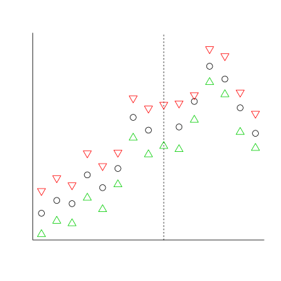
(b) The two primal estimators $r_{1}$ and $r_{2}$.

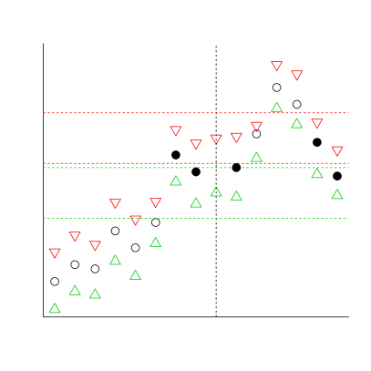
(c) The collective operates.

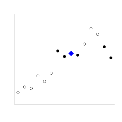
(d) Predicted value (diamond) for the query point $\mathbf{x}$.

We stress that the central and original idea behind our approach is that the resulting regression predictor is a nonlinear, nonparametric, data-dependent function of the basic predictors $r_{1},\dots,r_{M}$, where the predictors are used to determine a local distance between a new test instance and the original training data. To the best of our knowledge there exists no formalized procedure in the machine learning and aggregation literature that operates as ours does. In particular, note that the original nonparametric nature of our combined estimator opens up new perspectives of research.

Indeed, though we have in mind a batch setting where the data collected consists in an $n$-sample of i.i.d. replications of some variable $(\mathbf{X},Y)$, our procedure may be linked to other situations. For example, consider the case of functional data analysis (see Ferraty and Vieu, 2006, and Bongiorno et al., 2014, for a survey on recent developments). Even though our method is fitted for finite dimensional data, it may be naturally extended to functional data after a suitable preprocessing of the curves. For example, this can be achieved using an expansion of the curves on an appropriate functional dictionary, and/or via a variable selection approach, as in Aneiros and Vieu (2014). Note that in a recent work, Cholaquidis et al. (2015) adapts our procedure in a classification setting, also in a functional example.

Along with this paper, we release the software COBRA (Guedj, 2013) which implements the method as an additional package to the statistical software R (see R Core Team, 2014). COBRA is freely downloadable on the CRAN website. As detailed in Section 3, we undertook a lengthy series of numerical experiments, over which COBRA proved extremely successful. These stunning results lead us to believe that regression collectives can provide valuable insights on a wide range of prediction problems. Further, these same results demonstrate that COBRA has remarkable speed in terms of CPU timings. In the context of high-dimensional (such as genomic) data, such velocity is critical, and in fact COBRA can natively take advantage of multi-core parallel environments.

The paper is organized as follows. In Section 2, we describe the combined estimator—the regression collective—and derive a nonasymptotic risk bound. Next we present the main result, that is, the collective is asymptotically at least as good as any functional of the basic estimators. We also provide a rate of convergence for our procedure. Section 3 is devoted to the companion R package COBRA and presents benchmarks of its excellent performance on both simulated and real data sets, including high-dimensional models. We also show that COBRA compares favorably with two competitors, Super Learner (van der Laan et al., 2007) and the exponentially weighted aggregate (see for example Giraud, 2014), in that it performs similarly in most situations, much better in some, while it is consistently faster than the Super Learner in every case. Finally, for ease of exposition, proofs and additional simulation results (figures and tables with (SM) as suffix) are postponed to a Supplementary Material.

2 The combined estimator

2.1 Notation

Throughout the article, we assume that we are given a training sample denoted by $\mathcal{D}_{n}=\{(\mathbf{X}_{1},Y_{1}),\dots,(\mathbf{X}_{n},Y_{n})\}$. $\mathcal{D}_{n}$ is composed of i.i.d. random variables taking their values in $\mathbb{R}^{d}\times\mathbb{R}$, and distributed as an independent prototype pair $(\mathbf{X},Y)$ satisfying $\mathbb{E}Y^{2}<\infty$ (with the notation $\mathbf{X}=(X_{1},\dots,X_{d})$). The space $\mathbb{R}^{d}$ is equipped with the standard Euclidean metric. Our goal is to consistently estimate the regression function $r^{\star}(\mathbf{x})=\mathbb{E}[Y|\mathbf{X}=\mathbf{x}]$, $\mathbf{x}\in\mathbb{R}^{d}$, using the data $\mathcal{D}_{n}$.

To begin with, the original data set $\mathcal{D}_{n}$ is split into two data sequences $\mathcal{D}_{k}=\{(\mathbf{X}_{1},Y_{1}),\dots,(\mathbf{X}_{k},Y_{k})\}$ and $\mathcal{D}_{\ell}=\{(\mathbf{X}_{k+1},Y_{k+1}),\dots,(\mathbf{X}_{n},Y_{n})\}$, with $\ell=n-k\geq 1$. For ease of notation, the elements of $\mathcal{D}_{\ell}$ are renamed $\{(\mathbf{X}_{1},Y_{1}),\dots,(\mathbf{X}_{\ell},Y_{\ell})\}$. There is a slight abuse of notation here, as the same letter is used for both subsets $\mathcal{D}_{k}$ and $\mathcal{D}_{\ell}$—however, this should not cause any trouble since the context is clear.

Now, suppose that we are given a collection of $M\geq 1$ competing candidates $r_{k,1},\dots,r_{k,M}$ to estimate $r^{\star}$. These basic estimators—basic machines—are assumed to be generated using only the first subsample $\mathcal{D}_{k}$. These machines can be any among the researcher’s favorite toolkit, such as linear regression, kernel smoother, SVM, Lasso, neural networks, naive Bayes, or random forests. They could equally well be any ad hoc regression rules suggested by the experimental context. The essential idea is that these basic machines can be parametric, nonparametric, or semi-parametric, with possible tuning rules. All that is asked for is that each of the $r_{k,m}(\mathbf{x})$, $m=1,\dots,M$, is able to provide an estimation of $r^{\star}(\mathbf{x})$ on the basis of $\mathcal{D}_{k}$ alone. Thus, any collection of model-based or model-free machines are allowed, and our way of combining such a collection is here called the regression collective. Let us emphasize that the number of basic machines $M$ is considered as fixed throughout this paper. Hence, the number of machines is not expected to grow and is typically of a reasonable size ($M$ is chosen on the order of $10$ in Section 3).

Given the collection of basic machines $\mathbf{r}_{k}=(r_{k,1},\dots,r_{k,M})$, we define the collective estimator $T_{n}$ to be

$$T_{n}\left(\mathbf{r}_{k}(\mathbf{x})\right)=\sum_{i=1}^{\ell}W_{n,i}(\mathbf{x})Y_{i},\quad\mathbf{x}\in\mathbb{R}^{d},$$

where the random weights $W_{n,i}(\mathbf{x})$ take the form

$$W_{n,i}(\mathbf{x})=\frac{\mathbf{1}_{\bigcap_{m=1}^{M}\{|r_{k,m}(\mathbf{x})-r_{k,m}(\mathbf{X}_{i})|\leq\varepsilon_{\ell}\}}}{\sum_{j=1}^{\ell}\mathbf{1}_{\bigcap_{m=1}^{M}\{|r_{k,m}(\mathbf{x})-r_{k,m}(\mathbf{X}_{j})|\leq{\varepsilon}_{\ell}\}}}.$$ (2.1)

In this definition, ${\varepsilon}_{\ell}$ is some positive parameter and, by convention, $0/0=0$.

The weighting scheme used in our regression collective is distinctive but not obvious. Starting from Devroye et al. (1996) and Györfi et al. (2002), we see that $T_{n}$ is a local averaging estimator in the following sense: The predicted value for $r^{\star}(\mathbf{x})$, that is, the estimated outcome at the query point $\mathbf{x}$, is the unweighted average over those $Y_{i}$’s such that $\mathbf{X}_{i}$ is “close” to the query point. More precisely, for each $\mathbf{X}_{i}$ in the sample $\mathcal{D}_{\ell}$, “close” means that the output at the query point, generated from each basic machine, is within an $\varepsilon_{\ell}$-distance of the output generated by the same basic machine at $\mathbf{X}_{i}$. If a basic machine evaluated at $\mathbf{X}_{i}$ is close to the basic machine evaluated at the query point $\mathbf{x}$, then the corresponding outcome $Y_{i}$ is included in the average, and not otherwise. Also, as a further note of clarification: “Closeness” of the $\mathbf{X}_{i}$’s is not here to be understood in the Euclidean sense. It refers to closeness of the primal estimators outputs at the query point as compared to the outputs over all points in the training data. Training points $\mathbf{X}_{i}$ that are close, in this sense, to the corresponding outputs at the query point contribute to the indicator function for the corresponding outcome $Y_{i}$. This alternative approach is motivated by the fact that a major issue in learning problems consists of devising a metric that is suited to the data (see, e.g., the monograph by Pekalska and Duin, 2005).

In this context, $\varepsilon_{\ell}$ plays the role of a smoothing parameter: Put differently, in order to retain $Y_{i}$, all basic estimators $r_{k,1},\dots,r_{k,M}$ have to deliver predictions for the query point $\mathbf{x}$ which are in a $\varepsilon_{\ell}$-neighborhood of the predictions $r_{k,1}(\mathbf{X}_{i}),\dots,r_{k,M}(\mathbf{X}_{i})$. Note that the greater $\varepsilon_{\ell}$, the more tolerant the process. It turns out that the practical performance of $T_{n}$ strongly relies on an appropriate choice of $\varepsilon_{\ell}$. This important question will be discussed in Section 3, where we devise an automatic (i.e., data-dependent) selection strategy of $\varepsilon_{\ell}$.

Next, we note that the subscript $n$ in $T_{n}$ may be a little confusing, since $T_{n}$ is a weighted average of the $Y_{i}$’s in $\mathcal{D}_{\ell}$ only. However, $T_{n}$ depends on the entire data set $\mathcal{D}_{n}$, as the rest of the data is used to set up the original machines $r_{k,1},\dots,r_{k,M}$. Most importantly, it should be noticed that the combined estimator $T_{n}$ is nonlinear with respect to the basic estimators $r_{k,m}$. As such, it is inspired by the preliminary work of Mojirsheibani (1999) in the supervised classification context.

In addition, let us mention that, in the definition of the weights (2.1), all original estimators are invited to have the same, equally valued opinion on the importance of the observation $\mathbf{X}_{i}$ (within the range of $\varepsilon_{\ell}$) for the corresponding $Y_{i}$ to be integrated in the combination $T_{n}$. However, this unanimity constraint may be relaxed by imposing, for example, that a fixed fraction $\alpha\in\{1/M,2/M,\dots,1\}$ of the machines agrees on the importance of $\mathbf{X}_{i}$. In that case, the weights take the more sophisticated form

$$W_{n,i}(\mathbf{x})=\frac{\mathbf{1}_{\{\sum_{m=1}^{M}\mathbf{1}_{\{|r_{k,m}(\mathbf{x})-r_{k,m}(\mathbf{X}_{i})|\leq\varepsilon_{\ell}\}}\geq M\alpha\}}}{\sum_{j=1}^{\ell}{\mathbf{1}_{\{\sum_{m=1}^{M}\mathbf{1}_{\{|r_{k,m}(\mathbf{x})-r_{k,m}(\mathbf{X}_{j})|\leq\varepsilon_{\ell}\}}\geq M\alpha\}}}}.$$

It turns out that adding the parameter $\alpha$ does not change the asymptotic properties of $T_{n}$, provided $\alpha\to 1$. Thus, to keep a sufficient degree of clarity in the mathematical statements and subsequent proofs, we have decided to consider only the case $\alpha=1$ (i.e., unanimity). Extension of the results to more general values of $\alpha$ is left for future work. On the other hand, as highligthed by Section 3, $\alpha$ has a nonnegligible impact on the performance of the combined estimator. Accordingly, we will discuss in Section 3 an automatic procedure to select this extra parameter.

2.2 Theoretical performance

This section is devoted to the study of some asymptotic and nonasymptotic properties of the combined estimator $T_{n}$, whose quality will be assessed by the quadratic risk

$$\mathbb{E}\left|T_{n}\left(\mathbf{r}_{k}(\mathbf{X})\right)-r^{\star}(\mathbf{X})\right|^{2}.$$

Here and later, $\mathbb{E}$ denotes the expectation with respect to both $\mathbf{X}$ and the sample $\mathcal{D}_{n}$. Everywhere in the document, it is assumed that $\mathbb{E}|r_{k,m}(\mathbf{X})|^{2}<\infty$ for all $m=1,\dots,M$.

For any $m=1,\dots,M$, let $r_{k,m}^{-1}$ denote the inverse image of machine $r_{k,m}$. Assume that for any $m=1,\dots,M$,

$$r_{k,m}^{-1}((t,+\infty))\underset{t\uparrow+\infty}{\searrow}\emptyset\quad\mbox{and}\quad r_{k,m}^{-1}((-\infty,t))\underset{t\downarrow-\infty}{\searrow}\emptyset.$$ (2.2)

It is stressed that this is a mild assumption which is met, for example, whenever the machines are bounded. Throughout, we let

$$T\left(\mathbf{r}_{k}(\mathbf{X})\right)=\mathbb{E}\left[Y|\mathbf{r}_{k}(\mathbf{X})\right]$$

and note that, by the very definition of the $L^{2}$ conditional expectation,

$$\mathbb{E}\left|T(\mathbf{r}_{k}(\mathbf{X}))-Y\right|^{2}\leq\inf_{f}\ \mathbb{E}\left|f(\mathbf{r}_{k}(\mathbf{X}))-Y\right|^{2},$$ (2.3)

where the infimum is taken over all square integrable functions of $\mathbf{r}_{k}(\mathbf{X})$.

Our first result is a nonasymptotic inequality, which states that the combined estimator behaves as well as the best one in the original list, within a term measuring how far $T_{n}$ is from $T$.

Proposition 2.1.

Let $\mathbf{r}_{k}=(r_{k,1},\dots,r_{k,M})$ be the collection of basic estimators, and let $T_{n}(\mathbf{r}_{k}(\mathbf{x}))$ be the combined estimator. Then, for all distributions of $(\mathbf{X},Y)$ with $\mathbb{E}Y^{2}<\infty$,

$$\mathbb{E}| T_{n}(\mathbf{r}_{k}(\mathbf{X}))-r^{\star}(\mathbf{X})|^{2}$$

$$\leq\mathbb{E}|T_{n}(\mathbf{r}_{k}(\mathbf{X}))-T(\mathbf{r}_{k}(\mathbf{X}))|^{2}+\inf_{f}\ \mathbb{E}|f(\mathbf{r}_{k}(\mathbf{X}))-r^{\star}(\mathbf{X})|^{2},$$

where the infimum is taken over all square integrable functions of $\mathbf{r}_{k}(\mathbf{X})$. In particular,

$$\mathbb{E}|T_{n}(\mathbf{r}_{k}(\mathbf{X}))-r^{\star}(\mathbf{X})|^{2}$$

$$\quad\leq\min_{m=1,\dots,M}\mathbb{E}|r_{k,m}(\mathbf{X})-r^{\star}(\mathbf{X})|^{2}+\mathbb{E}|T_{n}(\mathbf{r}_{k}(\mathbf{X}))-T(\mathbf{r}_{k}(\mathbf{X}))|^{2}.$$

Proposition 2.1 guarantees the performance of $T_{n}$ with respect to the basic machines, whatever the distribution of $(\mathbf{X},Y)$ is and regardless of which initial estimator is actually the best. The term $\min_{m=1,\dots,M}\mathbb{E}|r_{k,m}(\mathbf{X})-r^{\star}(\mathbf{X})|^{2}$ may be regarded as a bias term, whereas the term $\mathbb{E}|T_{n}(\mathbf{r}_{k}(\mathbf{X}))-T(\mathbf{r}_{k}(\mathbf{X}))|^{2}$ is a variance-type term, which can be asymptotically neglected, as shown by the following result.

Proposition 2.2.

Assume that $\varepsilon_{\ell}\to 0$ and $\ell\varepsilon_{\ell}^{M}\to\infty$ as $\ell\to\infty.$ Then

$$\mathbb{E}\left|T_{n}\left(\mathbf{r}_{k}(\mathbf{X})\right)-T\left(\mathbf{r}_{k}(\mathbf{X})\right)\right|^{2}\to 0\quad\mbox{as }\ell\to\infty,$$

for all distributions of $(\mathbf{X},Y)$ with $\mathbb{E}Y^{2}<\infty$. Thus,

$$\limsup_{\ell\to\infty}\mathbb{E}\left|T_{n}\left(\mathbf{r}_{k}(\mathbf{X})\right)-r^{\star}(\mathbf{X})\right|^{2}\leq\inf_{f}\ \mathbb{E}\left|f(r_{k,m}(\mathbf{X}))-r^{\star}(\mathbf{X})\right|^{2}.$$

In particular,

$$\limsup_{\ell\to\infty}\mathbb{E}\left|T_{n}\left(\mathbf{r}_{k}(\mathbf{X})\right)-r^{\star}(\mathbf{X})\right|^{2}\leq\min_{m=1,\dots,M}\mathbb{E}\left|r_{k,m}(\mathbf{X})-r^{\star}(\mathbf{X})\right|^{2}.$$

This result is remarkable, for two reasons. Firstly, it shows that, in terms of predictive quadratic risk, the combined estimator does asymptotically at least as well as the best primitive machine. Secondly, the result is nearly universal, in the sense that it is true for all distributions of $(\mathbf{X},Y)$ such that $\mathbb{E}Y^{2}<\infty$.

This is especially interesting because the performance of any estimation procedure eventually depends upon some model and smoothness assumptions on the observations. For example, a linear regression fit performs well if the distribution is truly linear, but may behave poorly otherwise. Similarly, the Lasso procedure is known to do a good job for non-correlated designs, with no clear guarantee however in adversarial situations. Likewise, performance of nonparametric procedures such as the $k$-nearest neighbor method, kernel estimators and random forests dramatically deteriorate as the ambient dimension increases, but may be significantly improved if the true underlying dimension is reasonable. Note that this phenomenon is thoroughly analyzed for the random forests algorithm in Biau (2012).

The result exhibited in Proposition 2.2 holds under a minimal regularity assumption on the basic machines. However, this universality comes at a price since we have no guarantee on the rate of convergence of the variance term. Nevertheless, assuming some light additional smoothness conditions, one has the following result, which is the central statement of the paper.

Theorem 2.1.

Assume that $Y$ and the basic machines $\mathbf{r}_{k}$ are bounded by some constant $R$. Assume moreover that there exists a constant $L\geq 0$ such that, for every $k\geq 1$,

$$|T(\mathbf{r}_{k}(\mathbf{x}))-T(\mathbf{r}_{k}(\mathbf{y}))|\leq L|\mathbf{r}_{k}(\mathbf{x})-\mathbf{r}_{k}(\mathbf{y})|,\quad\mathbf{x},\mathbf{y}\in\mathbb{R}^{d}.$$

Then, with the choice $\varepsilon_{\ell}\propto\ell^{-\frac{1}{M+2}}$, one has

$$\mathbb{E}\left|T_{n}\left(\mathbf{r}_{k}(\mathbf{X})\right)-r^{\star}(\mathbf{X})\right|^{2}\leq\min_{m=1,\dots,M}\mathbb{E}\left|r_{k,m}(\mathbf{X})-r^{\star}(\mathbf{X})\right|^{2}+C\ell^{-\frac{2}{M+2}},$$

for some positive constant $C=C(R,L)$, independent of $k$.

Theorem 2.1 offers an oracle-type inequality with leading constant $1$ (i.e., sharp oracle inequality), stating that the risk of the regression collective is bounded by the lowest risk among those of the basic machines, i.e., our procedure mimics the performance of the oracle over the set $\{r_{k,m}\colon m=1,\dots,M\}$, plus a remainder term of the order of $\ell^{-2/(M+2)}$ which is the price to pay for combining $M$ estimators. In our setting, it is important to observe that this term has a limited impact. As a matter of fact, since the number of basic machines $M$ is assumed to be fixed and not too large (the implementation presented in Section 3 considers $M$ at most $6$), the remainder term is negligible compared to the standard nonparametric rate $\ell^{-2/(d+2)}$ in dimension $d$. While the rate $\ell^{-2/(d+2)}$ is affected by the curse of dimensionality when $d$ is large, this is not the case for the term $\ell^{-2/(M+2)}$. That way, our procedure appears well armed to face high dimensional problems. When $d\gg n$, many methods deteriorate and suffer from the curse of dimensionality. However, it is important to note here that even if some of the basic machines $r_{k,1},\dots,r_{k,M}$ might be less performant in that context, this does not affect in any way our combining procedure. Indeed, forming the regression collective $T_{n}$ does not require any additional effort if $d$ grows. Obviously, when $d$ is large, the best choice would be to include as basic machines methods and models which are adapted to the high dimensional setting. This is an interesting track for future research, which is connected to functional data analysis and dimension-reduction models (see Goia and Vieu, 2014).

Obviously, under the assumption that the distribution of $(\mathbf{X},Y)$ might be described parametrically and that one of the initial estimators is adapted to this distribution, faster rates of the order of $1/\ell$ could emerge in the bias term. Nonetheless, the regression collective is designed for much more adversarial regression problems, hence the rate exhibited in Theorem 2.1 appears satisfactory. We stress that our approach carries no assumption on the random design and mild ones over the primal estimators, in line with our attempt to design a procedure which is as model-free as possible.

The central motivation for our method is that model and smoothness assumptions are usually unverifiable, especially in modern high-dimensional and large scale data sets. To circumvent this difficulty, researchers often try many different methods and retain the one exhibiting the best empirical (e.g., cross-validated) results. Our combining strategy offers a nice alternative, in the sense that if one of the initial estimators is consistent for a given class $\mathcal{M}$ of distributions, then, under light smoothness assumptions, $T_{n}$ inherits the same property. To be more precise, assume that the initial pool of estimators includes a consistent estimator, i.e., that one of the original estimators, say $r_{k,m_{0}}$, satisfies

$$\mathbb{E}\left|r_{k,m_{0}}(\mathbf{X})-r^{\star}(\mathbf{X})\right|^{2}\to 0\quad\mbox{as }k\to\infty,$$

for all distributions of $(\mathbf{X},Y)$ in some class $\mathcal{M}$. Then, under the assumptions of Theorem 2.1, with the choice $\varepsilon_{\ell}\propto\ell^{-\frac{1}{M+2}}$, one has

$$\lim_{k,\ell\to\infty}\mathbb{E}\left|T_{n}\left(\mathbf{r}_{k}(\mathbf{X})\right)-r^{\star}(\mathbf{X})\right|^{2}=0.$$

3 Implementation and numerical studies

This section is devoted to the implementation of the described method. Its excellent performance is then assessed in a series of experiments. The companion R package COBRA (standing for COmBined Regression Alternative) is available on the CRAN website, for Linux, Mac and Windows platforms (see Guedj, 2013). Note that in a will to favor its execution speed, COBRA includes a parallel option, allowing for improved performance on multi-core computers (from Knaus, 2010).

As raised in the previous section, a precise calibration of the smoothing parameter $\varepsilon_{\ell}$ is crucial. Clearly, a value that is too small will discard many machines and most weights will be zero. Conversely, a large value sets all weights to $1/\Sigma$ with

$$\Sigma=\sum_{j=1}^{\ell}\mathbf{1}_{\bigcap_{m=1}^{M}\{|r_{k,m}(\mathbf{x})-r_{k,m}(\mathbf{X}_{j})|\leq{\varepsilon}_{\ell}\}},$$

giving the naive predictor that does not account for any new data point and predicts the mean over the sample $\mathcal{D}_{\ell}$. We also consider a relaxed version of the unanimity constraint: Instead of requiring global agreement over the implemented machines, consider some $\alpha\in(0,1]$ and keep observation $Y_{i}$ in the construction of $T_{n}$ if and only if at least a proportion $\alpha$ of the machines agrees on the importance of $\mathbf{X}_{i}$. This parameter requires some calibration. To understand this better, consider the following toy example: On some data set, assume most machines but one have nice predictive performance. For any new data point, requiring global agreement will fail since the pool of machines is heterogeneous. In this regard, $\alpha$ should be seen as a measure of homogeneity: If a small value is selected, it may be an indicator that some machines perform (possibly much) better than some others. Conversely, a large value indicates that the predictive abilities of the machines are close.

A natural measure of the risk in the prediction context is the empirical quadratic loss, namely

$$\hat{R}(\hat{\mathbf{Y}})=\frac{1}{p}\sum_{j=1}^{p}(\hat{Y}_{j}-Y_{j})^{2},$$

where $\hat{\mathbf{Y}}=(\hat{Y}_{1},\dots,\hat{Y}_{p})$ is the vector of predicted values for the responses $Y_{1},\dots,Y_{p}$ and $\{(\mathbf{X}_{j},Y_{j})\}_{j=1}^{p}$ is a testing sample. We adopted the following protocol: Using a simple data-splitting device, $\varepsilon_{\ell}$ and $\alpha$ are chosen by minimizing the empirical risk $\hat{R}$ over the set $\{\varepsilon_{\ell,\mathrm{min}},\dots,\varepsilon_{\ell,\mathrm{max}}\}\times\{1/M,\dots,1\}$, where $\varepsilon_{\ell,\mathrm{min}}=10^{-300}$ and $\varepsilon_{\ell,\mathrm{max}}$ is proportional to the largest absolute difference between two predictions of the pool of machines.

In the package, the number $\#\{\varepsilon_{\ell,\mathrm{min}},\dots,\varepsilon_{\ell,\mathrm{max}}\}$ of evaluated values may be modified by the user, otherwise the default value $200$ is chosen. It is also possible to choose either a linear or a logistic scale. Figure 2 (SM) illustrates the discussion about the choice of $\varepsilon_{\ell}$ and $\alpha$.

By default, COBRA includes the following classical packages dealing with regression estimation and prediction. However, note that the user has the choice to modify this list to her/his own convenience:

• Lasso (R package lars, see Hastie and Efron, 2012).

• Ridge regression (R package ridge, see Cule, 2012).

• $k$-nearest neighbors (R package FNN, see Li, 2013).

• CART algorithm (R package tree, see Ripley, 2012).

• Random Forests algorithm (R package randomForest, see Liaw and Wiener, 2002).

First, COBRA is benchmarked on synthetic data. For each of the following eight models, two designs are considered: Uniform over $(-1,1)^{d}$ (referred to as “Uncorrelated” in Table 1, Table 3 and Table 3), and Gaussian with mean $0$ and covariance matrix $\Sigma$ with $\Sigma_{ij}=2^{-|i-j|}$ (“Correlated”). Models considered cover a wide spectrum of contemporary regression problems. Indeed, Model 1 is a toy example, Model 2 comes from van der Laan et al. (2007), Model 3 and Model 4 appear in Meier et al. (2009). Model 5 is somewhat a classic setting. Model 6 is about predicting labels, Model 7 is inspired by high-dimensional sparse regression problems. Finally, Model 8 deals with probability estimation, forming a link with nonparametric model-free approaches such as in Malley et al. (2012). In the sequel, we let $\mathcal{N}(\mu,\sigma^{2})$ denote a Gaussian random variable with mean $\mu$ and variance $\sigma^{2}$. In the simulations, the training data set was usually set to $80\%$ of the whole sample, then split into two equal parts corresponding to $\mathcal{D}_{k}$ and $\mathcal{D}_{\ell}$.

Model 1.

$n=800$, $d=50$, $Y=X_{1}^{2}+\exp(-X_{2}^{2})$.

Model 2.

$n=600$, $d=100$, $Y=X_{1}X_{2}+X_{3}^{2}-X_{4}X_{7}+X_{8}X_{10}-X_{6}^{2}+\mathcal{N}(0,0.5)$.

Model 3.

$n=600$, $d=100$, $Y=-\sin(2X_{1})+X_{2}^{2}+X_{3}-\exp(-X_{4})+\mathcal{N}(0,0.5)$.

Model 4.

$n=600$, $d=100$, $Y=X_{1}+(2X_{2}-1)^{2}+\sin(2\pi X_{3})/(2-\sin(2\pi X_{3}))+\sin(2\pi X_{4})+2\cos(2\pi X_{4})+3\sin^{2}(2\pi X_{4})+4\cos^{2}(2\pi X_{4})+\mathcal{N}(0,0.5)$.

Model 5.

$n=700$, $d=20$, $Y=\mathbf{1}_{\{X_{1}>0\}}+X_{2}^{3}+\mathbf{1}_{\{X_{4}+X_{6}-X_{8}-X_{9}>1+X_{14}\}}+\exp(-X_{2}^{2})+\mathcal{N}(0,0.5)$.

Model 6.

$n=500$, $d=30$, $Y=\sum_{k=1}^{10}\mathbf{1}_{\{X^{3}_{k}<0\}}-\mathbf{1}_{\{\mathcal{N}(0,1)>1.25\}}$.

Model 7.

$n=600$, $d=300$, $Y=X_{1}^{2}+X_{2}^{2}X_{3}\exp(-|X_{4}|)+X_{6}-X_{8}+\mathcal{N}(0,0.5)$.

Model 8.

$n=600$, $d=50$, $Y=\mathbf{1}_{\{X_{1}+X_{4}^{3}+X_{9}+\sin(X_{12}X_{18})+\mathcal{N}(0,0.1)>0.38\}}$.

Table 1 presents the empirical mean quadratic error and standard deviation over $100$ independent replications, for each model and design. Bold numbers identify the lowest error, i.e., the apparent best competitor. Boxplots of errors are presented in Figure 3 (SM) and Figure 4 (SM). Further, Figure 5 (SM) and Figure 6 (SM) show the predictive capacities of COBRA, and Figure 7 (SM) depicts its ability to reconstruct the functional dependence over the covariates in the context of additive regression, assessing the striking performance of our approach in a wide spectrum of statistical settings. A persistent and notable fact is that COBRA performs at least as well as the best machine, especially so in Model 3, Model 5 and Model 6.

Next, since more and more problems in contemporary statistics involve high-dimensional data, we have tested the abilities of COBRA in that context. As highlighted by Table 4 (SM) and Figure 8 (SM), the main message is that COBRA is perfectly able to deal with high-dimensional data, provided that it is generated over machines, at least some of which are known to perform well in such situations (possibly at the price of a sparsity assumption). In that context, we conducted $200$ independent replications for the three following models:

Model 9.

$n=500$, $d=1000$, $Y=X_{1}+3X_{3}^{2}-2\exp(-X_{5})+X_{6}$. Uncorrelated design.

Model 10.

$n=500$, $d=1000$, $Y=X_{1}+3X_{3}^{2}-2\exp(-X_{5})+X_{6}$. Correlated design.

Model 11.

$n=500$, $d=1500$, $Y=\exp(-X_{1})+\exp(X_{1})+\sum_{j=2}^{d}X_{j}^{j/100}$. Uncorrelated design.

A legitimate question that arises is where one should cut the initial sample $\mathcal{D}_{n}$? In other words, for a given data set of size $n$, what is the optimal value for $k$? A naive approach is to cut the initial sample in two halfs (i.e., $k=n/2$): This appears to be satisfactory provided that $n$ is large enough, which may be too much of an unrealistic assumption in numerous experimental settings. A more involved choice is to adopt a random cut scheme, where $k$ is chosen uniformly in $\{1,\dots,n\}$. Figure 9 (SM) presents the boxplots of errors of the five default machines and COBRA with that random cutting strategy, and also shows the risk of COBRA with respect to $k$. To illustrate this phenomenon, we tested a thousand random cuts on the following Model 12. As showed in Figure 9 (SM), for that particular model, the best value seems to be near $3n/4$.

Model 12.

$n=1200$, $d=10$, $Y=X_{1}+3X_{3}^{2}-2\exp(-X_{5})+X_{6}$. Uncorrelated design.

The average risk of COBRA on a thousand replications of Model 12 is $0.3124$. Since this delivered a thousand prediction vectors, a natural idea is to take their mean or median. The risk of the mean is $0.2306$, and the median has an even better risk ($0.2184$). Since a random cut scheme may generate some unstability, we advise practitioners to compute a few COBRA estimators, then compute the mean or median vector of their predictions.

Next, we compare COBRA to the Super Learner algorithm (Polley and van der Laan, 2012). This widely used algorithm was first described in van der Laan et al. (2007) and extended in Polley and van der Laan (2010). Super Learner is used in this section as the key competitor to our method. In a nutshell, the Super Learner trains basic machines $r_{1},\dots,r_{M}$ on the whole sample $\mathcal{D}_{n}$. Then, following a $V$-fold cross-validation procedure, Super Learner adopts a $V$-blocks partition of the set $\{1,\dots,n\}$ and computes the matrix

$$H=(H_{ij})_{1\leq i\leq n}^{1\leq j\leq M},$$

where $H_{ij}$ is the prediction for the query point $\mathbf{X}_{i}$ made by machine $j$ trained on all remaining $V-1$ blocks, i.e., excluding the block containing $\mathbf{X}_{i}$. The Super Learner estimator is then

$$SL=\sum_{j=1}^{M}\hat{\alpha}_{j}r_{j},$$

where

$$\hat{\alpha}\in\underset{\alpha\in\Lambda^{M}}{\arg\inf}\sum_{i=1}^{n}|Y_{i}-(H\alpha)_{i}|^{2},$$

with $\Lambda^{M}$ denoting the simplex

$$\Lambda^{M}=\left\{\alpha\in\mathbb{R}^{M}\colon\sum_{j=1}^{M}\alpha_{j}=1,\ \alpha_{j}\geq 0\textrm{ for any }j=1,\dots,M\right\}.$$

This convex aggregation scheme is significantly different from our collective approach. Yet, we feel close to the philosophy carried by the SuperLearner package, in that both methods allow the user to aggregate as many machines as desired, then combining them to deliver predictive outcomes. For that reason, it is reasonable to deploy Super Learner as a benchmark in our study of our collective approach.

Table 3 summarizes the performance of COBRA and SuperLearner (used with SL.randomForest, SL.ridge and SL.glmnet, for the fairness of the comparison) through the described protocol. Both methods compete on similar terms in most models, although COBRA proves much more efficient on correlated design in Model 2 and Model 4. This already remarkable result is to be stressed by the flexibility and velocity showed by COBRA. Indeed, as emphasized in Table 3 , without even using the parallel option, COBRA obtains similar or better results than SuperLearner roughly five times faster. Note also that COBRA suffers from a disadvantage: SuperLearner is built on the whole sample $\mathcal{D}_{n}$ whereas COBRA only uses $\ell<n$ data points. Finally, observe that the algorithmic cost of computing the random weights on $n_{\mathrm{test}}$ query points is $\ell\times M\times n_{\mathrm{test}}$ operations. In the package, those calculations are handled in C language for optimal speed performance.

Super Learner is a natural competitor on the implementation side. However, on the theoretical side, we do not assume that it should be the only benchmark. Thus, we compared COBRA to the popular exponentially weighted aggregate estimator (EWA, see Giraud, 2014). We implemented the following version of the EWA: For all preliminary estimators $r_{k,1},\dots,r_{k,M}$, their empirical risks $\hat{R}_{1},\dots,\hat{R}_{M}$ are computed on a subsample of $\mathcal{D}_{\ell}$ and the EWA is

$$\mathrm{EWA}_{\beta}\colon\mathbf{x}\mapsto\sum_{j=1}^{M}\hat{w}_{j}r_{k,j}(\mathbf{x}),\quad\mathbf{x}\in\mathbb{R}^{d},$$

where

$$\hat{w}_{j}=\frac{\exp(-\beta\hat{R}_{j})}{\sum_{i=1}^{M}\exp(-\beta\hat{R}_{i})},\quad j=1,\dots,M.$$

The temperature parameter $\beta>0$ is selected by minimizing the empirical risk of $\mathrm{EWA}_{\beta}$ over a data-based grid, in the same spirit as the selection of $\varepsilon_{\ell}$ and $\alpha$. We conducted $200$ independent replications, on Models 9 to 12. The conclusion is that COBRA outperforms the EWA estimator in some models, and delivers similar performance in others, as shown in Figure 10 (SM) and Table 5 (SM).

Finally, COBRA is used to process the following real-life data sets:

• Concrete Slump Test (see Yeh, 2007).

• Concrete Compressive Strength (see Yeh, 1998).

• Wine Quality (see Cortez et al., 2009). We point out that the Wine Quality data set involves supervised classification and leads naturally to a line of future research using COBRA over probability machines (see Malley et al., 2012).

The good predictive performance of COBRA is summarized in Figure 11 (SM) and errors are presented in Figure 12 (SM). For every data set, the sample is divided into a training set ($90\%$) and a testing set ($10\%$) on which the predictive performance is evaluated. Boxplots are obtained by randomly shuffling the data points a hundred times.

As a conclusion to this thorough experimental protocol, it is our belief that COBRA sets a new high standard of reference, a benchmark procedure, both in terms of performance and velocity, for prediction-oriented problems in the context of regression, including high-dimensional problems.

Supplementary Material
COBRA: A Combined Regression Strategy
by G. Biau, A. Fischer, B. Guedj and J. D. Malley

A Proofs

A.1 Proof of Proposition 2.1

We have

$$\mathbb{E}|T_{n}(\mathbf{r}_{k}(\mathbf{X}))-r^{\star}(\mathbf{X})|^{2} =\mathbb{E}|T_{n}(\mathbf{r}_{k}(\mathbf{X}))-T(\mathbf{r}_{k}(\mathbf{X}))|^{2}$$

$$\quad+\mathbb{E}|T(\mathbf{r}_{k}(\mathbf{X}))-r^{\star}(\mathbf{X})|^{2}$$

$$\quad-2\mathbb{E}[(T_{n}(\mathbf{r}_{k}(\mathbf{X}))-T(\mathbf{r}_{k}(\mathbf{X})))(T(\mathbf{r}_{k}(\mathbf{X}))-r^{\star}(\mathbf{X}))].$$

As for the double product, notice that

$$\mathbb{E}[(T_{n}(\mathbf{r}_{k}(\mathbf{X}))-T(\mathbf{r}_{k}(\mathbf{X})))(T(\mathbf{r}_{k}(\mathbf{X}))-r^{\star}(\mathbf{X}))]$$

$$\quad=\mathbb{E}\left[\mathbb{E}\left[(T_{n}(\mathbf{r}_{k}(\mathbf{X}))-T(\mathbf{r}_{k}(\mathbf{X})))(T(\mathbf{r}_{k}(\mathbf{X}))-r^{\star}(\mathbf{X}))|\mathbf{r}_{k}(\mathbf{X}),\mathcal{D}_{n}\right]\right]$$

$$\quad=\mathbb{E}\left[(T_{n}(\mathbf{r}_{k}(\mathbf{X}))-T(\mathbf{r}_{k}(\mathbf{X})))\mathbb{E}\left[T(\mathbf{r}_{k}(\mathbf{X}))-r^{\star}(\mathbf{X})|\mathbf{r}_{k}(\mathbf{X}),\mathcal{D}_{n}\right]\right].$$

But

$$\mathbb{E}[r^{\star}(\mathbf{X})|\mathbf{r}_{k}(\mathbf{X}),\mathcal{D}_{n}] =\mathbb{E}[r^{\star}(\mathbf{X})|\mathbf{r}_{k}(\mathbf{X})]$$

$$\quad(\mbox{by independence of $\mathbf{X}$ and $\mathcal{D}_{n}$})$$

$$=\mathbb{E}[\mathbb{E}[Y|\mathbf{X}]|\mathbf{r}_{k}(\mathbf{X})]$$

$$=\mathbb{E}[Y|\mathbf{r}_{k}(\mathbf{X})]$$

$$\quad(\mbox{since }\sigma(\mathbf{r}_{k}(\mathbf{X}))\subset\sigma(\mathbf{X}))$$

$$=T(\mathbf{r}_{k}(\mathbf{X})).$$

Consequently,

$$\mathbb{E}[(T_{n}(\mathbf{r}_{k}(\mathbf{X}))-T(\mathbf{r}_{k}(\mathbf{X})))(T(\mathbf{r}_{k}(\mathbf{X}))-r^{\star}(\mathbf{X}))]=0$$

and

$$\mathbb{E}|T_{n}(\mathbf{r}_{k}(\mathbf{X}))-r^{\star}(\mathbf{X})|^{2}=\mathbb{E}|T_{n}(\mathbf{r}_{k}(\mathbf{X}))-T(\mathbf{r}_{k}(\mathbf{X}))|^{2}+\mathbb{E}|T(\mathbf{r}_{k}(\mathbf{X}))-r^{\star}(\mathbf{X})|^{2}.$$

Thus, by definition of the conditional expectation, and using the fact that $T(\mathbf{r}_{k}(\mathbf{X}))=\mathbb{E}[r^{\star}(\mathbf{X})|\mathbf{r}_{k}(\mathbf{X})]$,

$$\mathbb{E}|T_{n}(\mathbf{r}_{k}(\mathbf{X}))-r^{\star}(\mathbf{X})|^{2}\leq\mathbb{E}|T_{n}(\mathbf{r}_{k}(\mathbf{X}))-T(\mathbf{r}_{k}(\mathbf{X}))|^{2}+\inf_{f}\mathbb{E}|f(\mathbf{r}_{k}(\mathbf{X}))-r^{\star}(\mathbf{X})|^{2},$$

where the infimum is taken over all square integrable functions of $\mathbf{r}_{k}(\mathbf{X})$. In particular,

$$\mathbb{E}|T_{n}(\mathbf{r}_{k}(\mathbf{X}))-r^{\star}(\mathbf{X})|^{2}$$

$$\quad\leq\min_{m=1,\dots,M}\mathbb{E}|r_{k,m}(\mathbf{X})-r^{\star}(\mathbf{X})|^{2}+\mathbb{E}|T_{n}(\mathbf{r}_{k}(\mathbf{X}))-T(\mathbf{r}_{k}(\mathbf{X}))|^{2},$$

as desired.

A.2 Proof of Proposition 2.2

Note that the second statement is an immediate consequence of the first statement and Proposition 2.1, therefore we only have to prove that

$$\mathbb{E}\left|T_{n}\left(\mathbf{r}_{k}(\mathbf{X})\right)-T\left(\mathbf{r}_{k}(\mathbf{X})\right)\right|^{2}\to 0\quad\mbox{as }\ell\to\infty.$$

We start with a technical lemma, whose proof can be found in the monograph by Györfi et al. (2002).

Lemma A.1.

Let $B(n,p)$ be a binomial random variable with parameters $n\geq 1$ and $p>0$. Then

$$\mathbb{E}\left[\frac{1}{1+B(n,p)}\right]\leq\frac{1}{p(n+1)}$$

and

$$\mathbb{E}\left[\frac{\mathbf{1}_{\{B(n,p)>0\}}}{B(n,p)}\right]\leq\frac{2}{p(n+1)}.$$

For all distributions of $(\mathbf{X},Y)$, using the elementary inequality $(a+b+c)^{2}\leq 3(a^{2}+b^{2}+c^{2})$, note that

$$\mathbb{E}|T_{n}(\mathbf{r}_{k}(\mathbf{X}))-T(\mathbf{r}_{k}(\mathbf{X}))|^{2}$$

$$\quad=\mathbb{E}\left|\sum_{i=1}^{\ell}W_{n,i}(\mathbf{X})\left(Y_{i}-T(\mathbf{r}_{k}(\mathbf{X}_{i}))+T(\mathbf{r}_{k}(\mathbf{X}_{i}))-T(\mathbf{r}_{k}(\mathbf{X}))+T(\mathbf{r}_{k}(\mathbf{X}))\right)\right.$$

$$\qquad\Bigg{.}-T(\mathbf{r}_{k}(\mathbf{X}))\Bigg{|}^{2}$$

$$\quad\leq 3\mathbb{E}\left|\sum_{i=1}^{\ell}W_{n,i}(\mathbf{X})(T(\mathbf{r}_{k}(\mathbf{X}_{i}))-T(\mathbf{r}_{k}(\mathbf{X})))\right|^{2}$$ (A.1)

$$\qquad+3\mathbb{E}\left|\sum_{i=1}^{\ell}W_{n,i}(\mathbf{X})(Y_{i}-T(\mathbf{r}_{k}(\mathbf{X}_{i})))\right|^{2}$$ (A.2)

$$\qquad+3\mathbb{E}\left|\left(\sum_{i=1}^{\ell}W_{n,i}(\mathbf{X})-1\right)T(\mathbf{r}_{k}(\mathbf{X}))\right|^{2}.$$ (A.3)

Consequently, to prove the proposition, it suffices to establish that (A.1), (A.2) and (A.3) tend to $0$ as $\ell$ tends to infinity. This is done, respectively, in Proposition A.1, Proposition A.2 and Proposition A.3 below.

Proposition A.1.

Under the assumptions of Proposition 2.2,

$$\lim_{\ell\to\infty}\mathbb{E}\left|\sum_{i=1}^{\ell}W_{n,i}(\mathbf{X})(T({\mathbf{r}}_{k}(\mathbf{X}_{i}))-T({\mathbf{r}}_{k}(\mathbf{X})))\right|^{2}=0.$$

Proof of Proposition A.1.

By the Cauchy-Schwarz inequality,

$$\mathbb{E}\left|\sum_{i=1}^{\ell}W_{n,i}(\mathbf{X})(T({\mathbf{r}}_{k}(\mathbf{X}_{i}))-T({\mathbf{r}}_{k}(\mathbf{X})))\right|^{2}$$

$$\quad=\mathbb{E}\left|\sum_{i=1}^{\ell}\sqrt{W_{n,i}(\mathbf{X})}\sqrt{W_{n,i}(\mathbf{X})}\left(T({\mathbf{r}}_{k}(\mathbf{X}_{i}))-T({\mathbf{r}}_{k}(\mathbf{X}))\right)\right|^{2}$$

$$\quad\leq\mathbb{E}\left[\sum_{j=1}^{\ell}W_{n,j}(\mathbf{X})\sum_{i=1}^{\ell}W_{n,i}(\mathbf{X})\left|T({\mathbf{r}}_{k}(\mathbf{X}_{i}))-T({\mathbf{r}}_{k}(\mathbf{X}))\right|^{2}\right]$$

$$\quad=\mathbb{E}\left[\sum_{i=1}^{\ell}W_{n,i}(\mathbf{X})\left|T({\mathbf{r}}_{k}(\mathbf{X}_{i}))-T({\mathbf{r}}_{k}(\mathbf{X}))\right|^{2}\right]$$

$$\quad:=A_{n}.$$

The function $T$ is such that $\mathbb{E}[T^{2}({\mathbf{r}}_{k}(\mathbf{X}))]<\infty$. Therefore, it can be approximated in an $L^{2}$ sense by a continuous function with compact support, say $\tilde{T}$ (see, e.g., Theorem A.1 in Györfi et al., 2002). More precisely, for any $\eta>0$, there exists a function $\tilde{T}$ such that

$$\mathbb{E}\left|T({\mathbf{r}}_{k}(\mathbf{X}))-\tilde{T}({\mathbf{r}}_{k}(\mathbf{X}))\right|^{2}<\eta.$$

Consequently, we obtain

$$A_{n} =\mathbb{E}\left[\sum_{i=1}^{\ell}W_{n,i}(\mathbf{X})|T({\mathbf{r}}_{k}(\mathbf{X}_{i}))-T({\mathbf{r}}_{k}(\mathbf{X}))|^{2}\right]$$

$$\leq 3\mathbb{E}\left[\sum_{i=1}^{\ell}W_{n,i}(\mathbf{X})|T({\mathbf{r}}_{k}(\mathbf{X}_{i}))-\tilde{T}({\mathbf{r}}_{k}(\mathbf{X}_{i}))|^{2}\right]$$

$$\quad+3\mathbb{E}\left[\sum_{i=1}^{\ell}W_{n,i}(\mathbf{X})|\tilde{T}({\mathbf{r}}_{k}(\mathbf{X}_{i}))-\tilde{T}({\mathbf{r}}_{k}(\mathbf{X}))|^{2}\right]$$

$$\quad+3\mathbb{E}\left[\sum_{i=1}^{\ell}W_{n,i}(\mathbf{X})|\tilde{T}({\mathbf{r}}_{k}(\mathbf{X}))-T({\mathbf{r}}_{k}(\mathbf{X}))|^{2}\right]$$

$$:=3A_{n1}+3A_{n2}+3A_{n3}.$$

Computation of $A_{n3}$

Thanks to the approximation of $T$ by $\tilde{T}$,

$$A_{n3} =\mathbb{E}\left[\sum_{i=1}^{\ell}W_{n,i}(\mathbf{X})|T({\mathbf{r}}_{k}(\mathbf{X}))-\tilde{T}({\mathbf{r}}_{k}(\mathbf{X}))|^{2}\right]$$

$$\leq\mathbb{E}\left|T({\mathbf{r}}_{k}(\mathbf{X}))-\tilde{T}({\mathbf{r}}_{k}(\mathbf{X}))\right|^{2}<\eta.$$

Computation of $A_{n1}$

Denote by $\mu$ the distribution of $\mathbf{X}$. Then,

$$A_{n1} =\mathbb{E}\left[\sum_{i=1}^{\ell}W_{n,i}(\mathbf{X})|\tilde{T}({\mathbf{r}}_{k}(\mathbf{X}_{i}))-T({\mathbf{r}}_{k}(\mathbf{X}_{i}))|^{2}\right]$$

$$=\ell\mathbb{E}\left[\frac{{\mathbf{1}}_{\bigcap_{m=1}^{M}\{|r_{k,m}(\mathbf{X})-r_{k,m}(\mathbf{X}_{1})|\leq\varepsilon_{\ell}\}}}{\sum_{j=1}^{\ell}{\mathbf{1}}_{\bigcap_{m=1}^{M}\{|r_{k,m}(\mathbf{X})-r_{k,m}(\mathbf{X}_{j})|\leq\varepsilon_{\ell}\}}}|\tilde{T}({\mathbf{r}}_{k}(\mathbf{X}_{1}))-T({\mathbf{r}}_{k}(\mathbf{X}_{1}))|^{2}\right].$$

$$=\ell\mathbb{E}\Bigg{\{}\int_{\mathbb{R}^{d}}|\tilde{T}({\mathbf{r}}_{k}(\mathbf{u}))-T({\mathbf{r}}_{k}(\mathbf{u}))|^{2}$$

$$\times\mathbb{E} \Bigg{[}\int_{\mathbb{R}^{d}}\frac{{\mathbf{1}}_{\bigcap_{m=1}^{M}\{|r_{k,m}(\mathbf{x})-r_{k,m}(\mathbf{u})|\leq\varepsilon_{\ell}\}}}{{\mathbf{1}}_{\bigcap_{m=1}^{M}\{|r_{k,m}(\mathbf{x})-r_{k,m}(\mathbf{u})|\leq\varepsilon_{\ell}\}}+\sum_{j=2}^{\ell}{\mathbf{1}}_{\bigcap_{m=1}^{M}\{|r_{k,m}(\mathbf{x})-r_{k,m}(\mathbf{X}_{j})|\leq\varepsilon_{\ell}\}}}\mu(\textrm{d}\mathbf{x})$$

$$\qquad\qquad\Bigg{|}\mathcal{D}_{k}\Bigg{]}\mu(\textrm{d}\mathbf{u})\Bigg{\}}.$$

Letting

$$A_{n1}^{\prime} =\mathbb{E}\Bigg{[}\int_{\mathbb{R}^{d}}\frac{{\mathbf{1}}_{\bigcap_{m=1}^{M}\{|r_{k,m}(\mathbf{x})-r_{k,m}(\mathbf{u})|\leq\varepsilon_{\ell}\}}}{{\mathbf{1}}_{\bigcap_{m=1}^{M}\{|r_{k,m}(\mathbf{x})-r_{k,m}(\mathbf{u})|\leq\varepsilon_{\ell}\}}+\sum_{j=2}^{\ell}{\mathbf{1}}_{\bigcap_{m=1}^{M}\{|r_{k,m}(\mathbf{x})-r_{k,m}(\mathbf{X}_{j})|\leq\varepsilon_{\ell}\}}}\mu(\textrm{d}\mathbf{x})$$

$$\qquad\qquad\Bigg{|}\mathcal{D}_{k}\Bigg{]},$$

let us prove that $A_{n1}^{\prime}\leq\frac{2^{M}}{\ell}$. To this aim, observe that

$$A_{n1}^{\prime} =\mathbb{E}\left[\int_{\mathbb{R}^{d}}\frac{{\mathbf{1}}_{\{\mathbf{x}\in\bigcap_{m=1}^{M}r_{k,m}^{-1}([r_{k,m}(\mathbf{u})-\varepsilon_{\ell},r_{k,m}(\mathbf{u})+\varepsilon_{\ell}])\}}}{1+\sum_{j=2}^{\ell}{\mathbf{1}}_{\{\mathbf{X}_{j}\in\bigcap_{m=1}^{M}r_{k,m}^{-1}([r_{k,m}(\mathbf{x})-\varepsilon_{\ell},r_{k,m}(\mathbf{x})+\varepsilon_{\ell}])\}}}\mu(\textrm{d}\mathbf{x})\Bigg{|}\mathcal{D}_{k}\right]$$

$$=\mathbb{E}\left[\int_{\mathbb{R}^{d}}\frac{{\mathbf{1}}_{\{\mathbf{x}\in\bigcup_{(a_{1},\dots,a_{M})\in\{1,2\}^{M}}r_{k,1}^{-1}(I_{n,1}^{a_{1}}(\mathbf{u}))\cap\dots\cap r_{k,M}^{-1}(I_{n,M}^{a_{M}}(\mathbf{u}))\}}}{1+\sum_{j=2}^{\ell}{\mathbf{1}}_{\{\mathbf{X}_{j}\in\bigcap_{m=1}^{M}r_{k,m}^{-1}([r_{k,m}(\mathbf{x})-\varepsilon_{\ell},r_{k,m}(\mathbf{x})+\varepsilon_{\ell}])\}}}\mu(\textrm{d}\mathbf{x})\Bigg{|}\mathcal{D}_{k}\right]$$

$$\leq\sum_{p=1}^{2^{M}}\mathbb{E}\left[\int_{\mathbb{R}^{d}}\frac{{\mathbf{1}}_{\{\mathbf{x}\in R^{p}_{n}(\mathbf{u})\}}}{1+\sum_{j=2}^{\ell}{\mathbf{1}}_{\{\mathbf{X}_{j}\in\bigcap_{m=1}^{M}r_{k,m}^{-1}([r_{k,m}(\mathbf{x})-\varepsilon_{\ell},r_{k,m}(\mathbf{x})+\varepsilon_{\ell}])\}}}\mu(\textrm{d}\mathbf{x})\Bigg{|}\mathcal{D}_{k}\right].$$

Here, $I^{1}_{n,m}(\mathbf{u})=[r_{k,m}(\mathbf{u})-\varepsilon_{\ell},r_{k,m}(\mathbf{u})]$, $I^{2}_{n,m}(\mathbf{u})=[r_{k,m}(\mathbf{u}),r_{k,m}(\mathbf{u})+\varepsilon_{\ell}]$, and $R_{n}^{p}(\mathbf{u})$ is the $p$-th set of the form $r_{k,1}^{-1}(I_{n,1}^{a_{1}}(\mathbf{u}))\cap\dots\cap r_{k,M}^{-1}(I_{n,M}^{a_{M}}(\mathbf{u}))$ assuming that they have been ordered using the lexicographic order of $(a_{1},\dots,a_{M})$.

Next, note that

$$\mathbf{x}\in R_{n}^{p}(\mathbf{u})\Rightarrow R_{n}^{p}(\mathbf{u})\subset\bigcap_{m=1}^{M}r_{k,m}^{-1}([r_{k,m}(\mathbf{x})-\varepsilon_{\ell},r_{k,m}(\mathbf{x})+\varepsilon_{\ell}]).$$

To see this, just observe that, for all $m=1,\dots,M$, if $r_{k,m}(\mathbf{z})\in[r_{k,m}(\mathbf{u})-\varepsilon_{\ell},r_{k,m}(\mathbf{u})]$, i.e., $r_{k,m}(\mathbf{u})-\varepsilon_{\ell}\leq r_{k,m}(\mathbf{z})\leq r_{k,m}(\mathbf{u})$, then, as $r_{k,m}(\mathbf{u})-\varepsilon_{\ell}\leq r_{k,m}(\mathbf{x})\leq r_{k,m}(\mathbf{u})$, one has $r_{k,m}(\mathbf{x})-\varepsilon_{\ell}\leq r_{k,m}(\mathbf{z})\leq r_{k,m}(\mathbf{x})+\varepsilon_{\ell}$. Similarly, if $r_{k,m}(\mathbf{u})\leq r_{k,m}(\mathbf{z})\leq r_{k,m}(\mathbf{u})+\varepsilon_{\ell}$, then $r_{k,m}(\mathbf{u})\leq r_{k,m}(\mathbf{x})\leq r_{k,m}(\mathbf{u})+\varepsilon_{\ell}$ implies $r_{k,m}(\mathbf{x})-\varepsilon_{\ell}\leq r_{k,m}(\mathbf{z})\leq r_{k,m}(\mathbf{x})+\varepsilon_{\ell}$. Consequently,

$$A_{n1}^{\prime} \leq\sum_{p=1}^{2^{M}}\mathbb{E}\left[\int_{\mathbb{R}^{d}}\frac{{\mathbf{1}}_{\{\mathbf{x}\in R^{p}_{n}(\mathbf{u})\}}}{1+\sum_{j=2}^{\ell}{\mathbf{1}}_{\{\mathbf{X}_{j}\in R^{p}_{n}(\mathbf{u})\}}}\mu(\textrm{d}\mathbf{x})\Bigg{|}\mathcal{D}_{k}\right]$$

$$=\sum_{p=1}^{2^{M}}\mathbb{E}\left[\frac{\mu{\{R^{p}_{n}(\mathbf{u})\}}}{1+\sum_{j=2}^{\ell}{\mathbf{1}}_{\{\mathbf{X}_{j}\in R^{p}_{n}(\mathbf{u})\}}}\Bigg{|}\mathcal{D}_{k}\right]$$

$$\leq\sum_{p=1}^{2^{M}}\mathbb{E}\left[\frac{\mu{\{R^{p}_{n}(\mathbf{u})\}}}{\ell\mu{\{R^{p}_{n}(\mathbf{u})\}}}\Bigg{|}\mathcal{D}_{k}\right]\$$

$$\leq\frac{2^{M}}{\ell}$$

(by the first statement of Lemma A.1). Thus, returning to $A_{n1}$, we obtain

$$A_{n1}\leq 2^{M}\mathbb{E}\left|\tilde{T}({\mathbf{r}}_{k}(\mathbf{X})-T({\mathbf{r}}_{k}(\mathbf{X})))\right|^{2}<2^{M}\eta.$$

Computation of $A_{n2}$

For any $\delta>0$, write

$$A_{n2} =\mathbb{E}\left[\sum_{i=1}^{\ell}W_{n,i}(\mathbf{X})|\tilde{T}(\mathbf{r}_{k}(\mathbf{X}_{i}))-\tilde{T}(\mathbf{r}_{k}(\mathbf{X}))|^{2}\right]$$

$$=\mathbb{E}\left[\sum_{i=1}^{\ell}W_{n,i}(\mathbf{X})|\tilde{T}(\mathbf{r}_{k}(\mathbf{X}_{i}))-\tilde{T}(\mathbf{r}_{k}(\mathbf{X}))|^{2}{\mathbf{1}}_{\bigcup_{m=1}^{M}\{|r_{k,m}(\mathbf{X})-r_{k,m}(\mathbf{X}_{i})|>\delta\}}\right]$$

$$\quad+\mathbb{E}\left[\sum_{i=1}^{\ell}W_{n,i}(\mathbf{X})|\tilde{T}(\mathbf{r}_{k}(\mathbf{X}_{i}))-\tilde{T}(\mathbf{r}_{k}(\mathbf{X}))|^{2}{\mathbf{1}}_{\bigcap_{m=1}^{M}\{|r_{k,m}(\mathbf{X})-r_{k,m}(\mathbf{X}_{i})|\leq\delta\}}\right]$$

from which we get that

$$A_{n2} \leq 4\sup_{\mathbf{u}\in\mathbb{R}^{d}}|\tilde{T}(\mathbf{r}_{k}(\mathbf{u}))|^{2}\mathbb{E}\left[\sum_{i=1}^{\ell}W_{n,i}(\mathbf{X}){\mathbf{1}}_{\bigcup_{m=1}^{M}\{|r_{k,m}(\mathbf{X})-r_{k,m}(\mathbf{X}_{i})|>\delta\}}\right]$$ (A.4)

$$\qquad+\bigg{(}\sup_{\mathbf{u},\mathbf{v}\in\mathbb{R}^{d},\bigcap_{m=1}^{M}\{|r_{k,m}(\mathbf{u})-r_{k,m}(\mathbf{v})|\leq\delta\}}|\tilde{T}(\mathbf{r}_{k}(\mathbf{v}))-\tilde{T}(\mathbf{r}_{k}(\mathbf{u}))|\bigg{)}^{2}.$$ (A.5)

With respect to the term $\eqref{eq:delta1}$, if $\delta>\varepsilon_{\ell}$, then

$$\sum_{i=1}^{\ell}W_{n,i}(\mathbf{X}){\mathbf{1}}_{\bigcup_{m=1}^{M}\{|r_{k,m}(\mathbf{X})-r_{k,m}(\mathbf{X}_{i})|>\delta\}}$$

$$\quad=\sum_{i=1}^{\ell}\frac{{\mathbf{1}}_{\bigcap_{m=1}^{M}\{|r_{k,m}(\mathbf{X})-r_{k,m}(\mathbf{X}_{i})|\leq\varepsilon_{\ell}\}}{\mathbf{1}}_{\bigcup_{m=1}^{M}\{|r_{k,m}(\mathbf{X})-r_{k,m}(\mathbf{X}_{i})|>\delta\}}}{\sum_{j=1}^{\ell}{\mathbf{1}}_{\bigcap_{m=1}^{M}\{|r_{k,m}(\mathbf{X})-r_{k,m}(\mathbf{X}_{j})|\leq\varepsilon_{\ell}\}}}$$

$$\quad=0.$$

It follows that, for all $\delta>0$, this term converges to 0 as $\ell$ tends to infinity. On the other hand, letting $\delta\to 0$, we see that the term $\eqref{eq:delta2}$ tends to 0 as well, by uniform continuity of $\tilde{T}$. Hence, $A_{n2}$ tends to 0 as $\ell$ tends to infinity. Letting finally $\eta$ go to 0, we conclude that $A_{n}$ vanishes as $\ell$ tends to infinity. ∎

Proposition A.2.

Under the assumptions of Proposition 2.2,

$$\lim_{\ell\to\infty}\mathbb{E}\left|\sum_{i=1}^{\ell}W_{n,i}(\mathbf{X})(Y_{i}-T(\mathbf{r}_{k}(\mathbf{X}_{i})))\right|^{2}=0.$$

Proof of Proposition A.2.

$$\mathbb{E}\left|\sum_{i=1}^{\ell}W_{n,i}(\mathbf{X})(Y_{i}-T(\mathbf{r}_{k}(\mathbf{X}_{i})))\right|^{2}$$

$$\quad=\sum_{i=1}^{\ell}\sum_{j=1}^{\ell}\mathbb{E}[W_{n,i}(\mathbf{X})W_{n,j}(\mathbf{X})(Y_{i}-T(\mathbf{r}_{k}(\mathbf{X}_{i})))(Y_{j}-T(\mathbf{r}_{k}(\mathbf{X}_{j})))]$$

$$\quad=\mathbb{E}\left[\sum_{i=1}^{\ell}W_{n,i}^{2}(\mathbf{X})|Y_{i}-T(\mathbf{r}_{k}(\mathbf{X}_{i}))|^{2}\right]$$

$$\quad=\mathbb{E}\left[\sum_{i=1}^{\ell}W_{n,i}^{2}(\mathbf{X})\sigma^{2}(\mathbf{r}_{k}(\mathbf{X}_{i}))\right],$$

where

$$\sigma^{2}(\mathbf{r}_{k}(\mathbf{x}))=\mathbb{E}[|Y-T(\mathbf{r}_{k}(\mathbf{X}))|^{2}|\mathbf{r}_{k}(\mathbf{x})].$$

For any $\eta>0$, $\sigma^{2}$ can be approximated in an $L^{1}$ sense by a continuous function with compact support $\tilde{\sigma}^{2}$, i.e.,

$$\mathbb{E}|\tilde{\sigma}^{2}(\mathbf{r}_{k}(\mathbf{X}))-\sigma^{2}(\mathbf{r}_{k}(\mathbf{X}))|<\eta.$$

Thus

$$\mathbb{E}\left[\sum_{i=1}^{\ell}W_{n,i}^{2}(\mathbf{X})\sigma^{2}(\mathbf{r}_{k}(\mathbf{X}_{i}))\right]$$

$$\quad\leq\mathbb{E}\left[\sum_{i=1}^{\ell}W^{2}_{n,i}(\mathbf{X})\tilde{\sigma}^{2}(\mathbf{r}_{k}(\mathbf{X}_{i}))\right]$$

$$\qquad+\mathbb{E}\left[\sum_{i=1}^{\ell}W^{2}_{n,i}(\mathbf{X})|\sigma^{2}(\mathbf{r}_{k}(\mathbf{X}_{i}))-\tilde{\sigma}^{2}(\mathbf{r}_{k}(\mathbf{X}_{i}))|\right]$$

$$\quad\leq\sup_{\mathbf{u}\in\mathbb{R}^{d}}|\tilde{\sigma}^{2}(\mathbf{r}_{k}(\mathbf{u}))|\mathbb{E}\left[\sum_{i=1}^{\ell}W_{n,i}^{2}(\mathbf{X})\right]$$

$$\qquad+\mathbb{E}\left[\sum_{i=1}^{\ell}W_{n,i}(\mathbf{X})|\sigma^{2}(\mathbf{r}_{k}(\mathbf{X}_{i}))-\tilde{\sigma}^{2}(\mathbf{r}_{k}(\mathbf{X}_{i}))|\right].$$

With the same argument as for $A_{n1}$, we obtain

$$\mathbb{E}\left[\sum_{i=1}^{\ell}W_{n,i}(\mathbf{X})|\sigma^{2}(\mathbf{r}_{k}(\mathbf{X}_{i}))-\tilde{\sigma}^{2}(\mathbf{r}_{k}(\mathbf{X}_{i}))|\right]\leq 2^{M}\eta.$$

Therefore, it remains to prove that $\mathbb{E}\left[\sum_{i=1}^{\ell}W_{n,i}^{2}(\mathbf{X})\right]\to 0$ as $\ell\to\infty$. To this aim, fix $\delta>0$, and note that

$$\sum_{i=1}^{\ell}W_{n,i}^{2}(\mathbf{X}) =\frac{\sum_{i=1}^{\ell}{\mathbf{1}}_{\bigcap_{m=1}^{M}\{|r_{k,m}(\mathbf{X})-r_{k,m}(\mathbf{X}_{i})|\leq\varepsilon_{\ell}\}}}{\left(\sum_{j=1}^{\ell}{\mathbf{1}}_{\bigcap_{m=1}^{M}\{|r_{k,m}(\mathbf{X})-r_{k,m}(\mathbf{X}_{j})|\leq\varepsilon_{\ell}\}}\right)^{2}}$$

$$\leq\min\left\{\delta,\frac{1}{\sum_{i=1}^{\ell}{\mathbf{1}}_{\bigcap_{m=1}^{M}\{|r_{k,m}(\mathbf{X})-r_{k,m}(\mathbf{X}_{i})|\leq\varepsilon_{\ell}\}}}\right\}$$

$$\leq\delta+\frac{{\mathbf{1}}_{\left\{\sum_{i=1}^{\ell}{\mathbf{1}}_{\bigcap_{m=1}^{M}\{|r_{k,m}(\mathbf{X})-r_{k,m}(\mathbf{X}_{i})|\leq\varepsilon_{\ell}\}}>0\right\}}}{\sum_{i=1}^{\ell}{\mathbf{1}}_{\bigcap_{m=1}^{M}\{|r_{k,m}(\mathbf{X})-r_{k,m}(\mathbf{X}_{i})|\leq\varepsilon_{\ell}\}}}.$$

To complete the proof, we have to establish that the expectation of the right-hand term tends to $0$. Denoting by $I$ a bounded interval on the real line, we have

$$\mathbb{E}\left[\frac{{\mathbf{1}}_{\left\{\sum_{i=1}^{\ell}{\mathbf{1}}_{\left\{\mathbf{X}_{i}\in\bigcap_{m=1}^{M}r_{k,m}^{-1}([r_{k,m}(\mathbf{X})-\varepsilon_{\ell},r_{k,m}(\mathbf{X})+\varepsilon_{\ell}])\right\}}>0\right\}}}{\sum_{i=1}^{\ell}{\mathbf{1}}_{\left\{\mathbf{X}_{i}\in\bigcap_{m=1}^{M}r_{k,m}^{-1}([r_{k,m}(\mathbf{X})-\varepsilon_{\ell},r_{k,m}(\mathbf{X})+\varepsilon_{\ell}])\right\}}}\right]$$

$$\leq\mathbb{E}\left[\frac{{\mathbf{1}}_{\left\{\sum_{i=1}^{\ell}{\mathbf{1}}_{\left\{\mathbf{X}_{i}\in\bigcap_{m=1}^{M}r_{k,m}^{-1}([r_{k,m}(\mathbf{X})-\varepsilon_{\ell},r_{k,m}(\mathbf{X})+\varepsilon_{\ell}])\right\}}>0\right\}}{\mathbf{1}}_{\left\{\mathbf{X}\in\bigcap_{m=1}^{M}r_{k,m}^{-1}(I)\right\}}}{\sum_{i=1}^{\ell}{\mathbf{1}}_{\left\{\mathbf{X}_{i}\in\bigcap_{m=1}^{M}r_{k,m}^{-1}([r_{k,m}(\mathbf{X})-\varepsilon_{\ell},r_{k,m}(\mathbf{X})+\varepsilon_{\ell}])\right\}}}\right]$$

$$\quad\quad+\mu\Big{(}\bigcup_{m=1}^{M}r_{k,m}^{-1}(I^{c})\Big{)}$$

$$=\mathbb{E}\left[\mathbb{E}\left[\frac{{\mathbf{1}}_{\left\{\sum_{i=1}^{\ell}{\mathbf{1}}_{\left\{\mathbf{X}_{i}\in\bigcap_{m=1}^{M}r_{k,m}^{-1}([r_{k,m}(\mathbf{X})-\varepsilon_{\ell},r_{k,m}(\mathbf{X})+\varepsilon_{\ell}])\right\}}>0\right\}}{\mathbf{1}}_{\left\{\mathbf{X}\in\bigcap_{m=1}^{M}r_{k,m}^{-1}(I)\right\}}}{\sum_{i=1}^{\ell}{\mathbf{1}}_{\left\{\mathbf{X}_{i}\in\bigcap_{m=1}^{M}r_{k,m}^{-1}([r_{k,m}(\mathbf{X})-\varepsilon_{\ell},r_{k,m}(\mathbf{X})+\varepsilon_{\ell}])\right\}}}\right.\right.$$

$$\qquad\left.\left.\Big{|}\mathcal{D}_{k},\mathbf{X}\right]\right]+\mu\Big{(}\bigcup_{m=1}^{M}r_{k,m}^{-1}(I^{c})\Big{)}$$

$$\leq\frac{2}{(\ell+1)}\mathbb{E}\left[\frac{{\mathbf{1}}_{\left\{\mathbf{X}\in\bigcap_{m=1}^{M}r_{k,m}^{-1}(I)\right\}}}{\mu(\bigcap_{m=1}^{M}r_{k,m}^{-1}([r_{k,m}(\mathbf{X})-\varepsilon_{\ell},r_{k,m}(\mathbf{X})+\varepsilon_{\ell}]))}\right]$$

$$\quad+\mu\Big{(}\bigcup_{m=1}^{M}r_{k,m}^{-1}(I^{c})\Big{)}.$$

The last inequality arises from the second statement of Lemma A.1. By an appropriate choice of $I$, according to the technical statement (2.2), the second term on the right-hand side can be made as small as desired. Regarding the first term, there exists a finite number $N_{\ell}$ of points $\mathbf{z}_{1},\dots,\mathbf{z}_{N_{\ell}}$ such that

$$\bigcap_{m=1}^{M}r_{k,m}^{-1}(I)\subset\bigcup_{(j_{1},\dots,j_{M})\in\{1,\dots,N_{\ell}\}^{M}}r_{k,1}^{-1}(I_{n,1}(\mathbf{z}_{j_{1}}))\cap\dots\cap r_{k,M}^{-1}(I_{n,M}(\mathbf{z}_{j_{M}})),$$

where $I_{n,m}(\mathbf{z}_{j})=[\mathbf{z}_{j}-\varepsilon_{\ell}/2,\mathbf{z}_{j}+\varepsilon_{\ell}/2]$. Suppose, without loss of generality, that the sets

$$r_{k,1}^{-1}(I_{n,1}(\mathbf{z}_{j_{1}}))\cap\dots\cap r_{k,M}^{-1}(I_{n,M}(\mathbf{z}_{j_{M}}))$$

are ordered, and denote by $R^{p}_{n}$ the $p$-th among the $N_{\ell}^{M}=(\lceil|I|/\varepsilon_{\ell}\rceil)^{M}$ sets. Here $|I|$ denotes the length of the interval $I$ and $\lceil x\rceil$ denotes the smallest integer greater than $x$. For all $p$,

$$\mathbf{x}\in R_{n}^{p}\Rightarrow R_{n}^{p}\subset\bigcap_{m=1}^{M}r_{k,m}^{-1}([r_{k,m}(\mathbf{x})-\varepsilon_{\ell},r_{k,m}(\mathbf{x})+\varepsilon_{\ell}]).$$

Indeed, if $\mathbf{v}\in R_{n}^{p}$, then, for all $m=1,\dots,M$, there exists $j\in\{1,\dots,N_{\ell}\}$ such that $r_{k,m}(\mathbf{v})\in[\mathbf{z}_{j}-\varepsilon_{\ell}/2,\mathbf{z}_{j}+\varepsilon_{\ell}/2]$, that is $\mathbf{z}_{j}-\varepsilon_{\ell}/2\leq r_{k,m}(\mathbf{v})\leq\mathbf{z}_{j}+\varepsilon_{\ell}/2$. Since we also have $\mathbf{z}_{j}-\varepsilon_{\ell}/2\leq r_{k,m}(\mathbf{X})\leq\mathbf{z}_{j}+\varepsilon_{\ell}/2$, we obtain $r_{k,m}(\mathbf{X})-\varepsilon_{\ell}\leq r_{k,m}(\mathbf{v})\leq r_{k,m}(\mathbf{X})+\varepsilon_{\ell}$. In conclusion,

$$\mathbb{E}\left[\frac{{\mathbf{1}}_{\left\{\mathbf{X}\in\bigcap_{m=1}^{M}r_{k,m}^{-1}(I)\right\}}}{\mu(\bigcap_{m=1}^{M}r_{k,m}^{-1}([r_{k,m}(\mathbf{X})-\varepsilon_{\ell},r_{k,m}(\mathbf{X})+\varepsilon_{\ell}]))}\right]$$

$$\quad\leq\sum_{p=1}^{N_{\ell}^{M}}\mathbb{E}\left[\frac{{\mathbf{1}}_{\left\{\mathbf{X}\in R_{n}^{p}\right\}}}{\mu(\bigcap_{m=1}^{M}r_{k,m}^{-1}([r_{k,m}(\mathbf{X})-\varepsilon_{\ell},r_{k,m}(\mathbf{X})+\varepsilon_{\ell}]))}\right]$$

$$\quad\leq\sum_{p=1}^{N_{\ell}^{M}}\mathbb{E}\left[\frac{{\mathbf{1}}_{\left\{\mathbf{X}\in R_{n}^{p}\right\}}}{\mu(R_{n}^{p})}\right]$$

$$\quad=N_{\ell}^{M}$$

$$\quad=\left\lceil\frac{|I|}{\varepsilon_{\ell}}\right\rceil^{M}.$$

The result follows from the assumption $\lim_{\ell\to\infty}\ell\varepsilon_{\ell}^{M}=\infty$. ∎

Proposition A.3.

Under the assumptions of Proposition 2.2,

$$\lim_{\ell\to\infty}\mathbb{E}\left|\left(\sum_{i=1}^{\ell}W_{n,i}(\mathbf{X})-1\right)T(\mathbf{r}_{k}(\mathbf{X}))\right|^{2}=0.$$

Proof of Proposition A.3.

Since $|\sum_{i=1}^{\ell}W_{n,i}(\mathbf{X})-1|\leq 1$, one has

$$\left|\left(\sum_{i=1}^{\ell}W_{n,i}(\mathbf{X})-1\right)T(\mathbf{r}_{k}(\mathbf{X}))\right|^{2}\leq T^{2}(\mathbf{r}_{k}(\mathbf{X})).$$

Consequently, by Lebesgue’s dominated convergence theorem, to prove the proposition, it suffices to show that $W_{n,i}(\mathbf{X})$ tends to 1 almost surely. Now,

$$\mathbb{P}\left(\sum_{i=1}^{\ell}W_{n,i}(\mathbf{X})\neq 1\right)$$

$$\quad=\mathbb{P}\left(\sum_{i=1}^{\ell}{\mathbf{1}}_{\bigcap_{m=1}^{M}\{|r_{k,m}(\mathbf{X})-r_{k,m}(\mathbf{X}_{i}))|\leq\varepsilon_{\ell}\}}=0\right)$$

$$\quad=\mathbb{P}\left(\sum_{i=1}^{\ell}{\mathbf{1}}_{\left\{\mathbf{X}_{i}\in\bigcap_{m=1}^{M}r_{k,m}^{-1}\left([r_{k,m}(\mathbf{X})-\varepsilon_{\ell},r_{k,m}(\mathbf{X})+\varepsilon_{\ell}]\right)\right\}}=0\right)$$

$$\quad=\int_{\mathbb{R}^{d}}\mathbb{P}\left(\forall i=1,\dots,\ell,{\mathbf{1}}_{\left\{\mathbf{X}_{i}\in\bigcap_{m=1}^{M}r_{k,m}^{-1}\left([r_{k,m}(\mathbf{x})-\varepsilon_{\ell},r_{k,m}(\mathbf{x})+\varepsilon_{\ell}]\right)\right\}}=0\right)\mu(\textrm{d}\mathbf{x})$$

$$\quad=\int_{\mathbb{R}^{d}}\left[1-\mu(\cap_{m=1}^{M}r_{k,m}^{-1}\left([r_{k,m}(\mathbf{x})-\varepsilon_{\ell},r_{k,m}(\mathbf{x})+\varepsilon_{\ell}]\right))\right]^{\ell}\mu(\textrm{d}\mathbf{x}).$$

Denote by $I$ a bounded interval. Then,

$$\mathbb{P}\left(\sum_{i=1}^{\ell}W_{n,i}(\mathbf{X})\neq 1\right)$$

$$\quad\leq\int_{\mathbb{R}^{d}}{\exp\left(-\ell\mu(\cap_{m=1}^{M}r_{k,m}^{-1}\left([r_{k,m}(\mathbf{x})-\varepsilon_{\ell},r_{k,m}(\mathbf{x})+\varepsilon_{\ell}]\right))\right)}$$

$$\qquad\times{\mathbf{1}}_{\{\mathbf{x}\in\bigcap_{m=1}^{M}r_{k,m}^{-1}(I)\}}\mu(\textrm{d}\mathbf{x})+\mu\Big{(}\bigcup_{m=1}^{M}r_{k,m}^{-1}(I^{c})\Big{)}$$

$$\quad\leq\max_{\mathbf{u}}\mathbf{u}e^{-\mathbf{u}}\int_{\mathbb{R}^{d}}\frac{{\mathbf{1}}_{\{\mathbf{x}\in\bigcap_{m=1}^{M}r_{k,m}^{-1}(I)\}}}{\ell\mu(\cap_{m=1}^{M}r_{k,m}^{-1}\left([r_{k,m}(\mathbf{x})-\varepsilon_{\ell},r_{k,m}(\mathbf{x})+\varepsilon_{\ell}]\right))}\mu(\textrm{d}\mathbf{x})$$

$$\qquad+\mu\Big{(}\bigcup_{m=1}^{M}r_{k,m}^{-1}(I^{c})\Big{)}.$$

Using the same arguments as in the proof of Proposition A.2, the probability $\mathbb{P}\left(\sum_{i=1}^{\ell}W_{n,i}(\mathbf{X})\neq 1\right)$ is bounded by $\frac{e^{-1}}{\ell}\left\lceil{\frac{|I|}{\varepsilon_{\ell}}}\right\rceil^{M}$. This bound vanishes as $n$ tends to infinity since, by assumption, $\lim_{\ell\to\infty}\ell\varepsilon_{\ell}^{M}=\infty$. ∎

A.3 Proof of Theorem 2.1

Choose $\mathbf{x}\in\mathbb{R}^{d}$. An easy calculation yields that

$$\mathbb{E}[|T_{n}(\mathbf{r}_{k}(\mathbf{x}))-T(\mathbf{r}_{k}(\mathbf{x}))|^{2}\big{|}\mathbf{r}_{k}(\mathbf{X}_{1}),\dots,\mathbf{r}_{k}(\mathbf{X}_{\ell}),\mathcal{D}_{k}]$$

$$=\mathbb{E}\Bigg{[}\big{|}T_{n}(\mathbf{r}_{k}(\mathbf{x}))-\mathbb{E}[T_{n}(\mathbf{r}_{k}(\mathbf{x}))\big{|}\mathbf{r}_{k}(\mathbf{X}_{1}),\dots,\mathbf{r}_{k}(\mathbf{X}_{\ell}),\mathcal{D}_{k}]\big{|}^{2}$$ (A.6)

$$\quad\Big{|}\mathbf{r}_{k}(\mathbf{X}_{1}),\dots,\mathbf{r}_{k}(\mathbf{X}_{\ell}),\mathcal{D}_{k}\Bigg{]}+\big{|}\mathbb{E}[T_{n}(\mathbf{r}_{k}(\mathbf{x}))\big{|}\mathbf{r}_{k}(\mathbf{X}_{1}),\dots,\mathbf{r}_{k}(\mathbf{X}_{\ell}),\mathcal{D}_{k}]-T(\mathbf{r}_{k}(\mathbf{x}))\big{|}^{2}$$

$$:=E_{1}+E_{2}.$$ (A.7)

On the one hand, we have

$$E_{1} =\mathbb{E}\Big{[}\big{|}T_{n}(\mathbf{r}_{k}(\mathbf{x}))-\mathbb{E}[T_{n}(\mathbf{r}_{k}(\mathbf{x}))|\mathbf{r}_{k}(\mathbf{X}_{1}),\dots,\mathbf{r}_{k}(\mathbf{X}_{\ell}),\mathcal{D}_{k}]\big{|}^{2}$$

$$\qquad\qquad\Big{|}\mathbf{r}_{k}(\mathbf{X}_{1}),\dots,\mathbf{r}_{k}(\mathbf{X}_{\ell}),\mathcal{D}_{k}\Big{]}$$

$$=\mathbb{E}\left[\left|\sum_{i=1}^{\ell}W_{n,i}(\mathbf{x})(Y_{i}-\mathbb{E}[Y_{i}|\mathbf{r}_{k}(\mathbf{X}_{i})])\right|^{2}|\mathbf{r}_{k}(\mathbf{X}_{1}),\dots,\mathbf{r}_{k}(\mathbf{X}_{\ell}),\mathcal{D}_{k}\right].$$

Developing the square and noticing that $\mathbb{E}\big{[}Y_{j}|Y_{i},\mathbf{r}_{k}(\mathbf{X}_{1}),\dots,\mathbf{r}_{k}(\mathbf{X}_{\ell}),\mathcal{D}_{k}\big{]}=\mathbb{E}[Y_{j}|\mathbf{r}_{k}(\mathbf{X}_{j})]$, since $Y_{j}$ is independent of $Y_{i}$ and of the $\mathbf{X}_{j}$’s with $j\neq i$, we have

$$E_{1} =\mathbb{E}\Bigg{[}\frac{\sum_{i=1}^{\ell}\mathbf{1}_{\bigcap_{m=1}^{M}\{|r_{k,m}(\mathbf{x})-r_{k,m}(\mathbf{X}_{i})|\leq\varepsilon_{\ell}\}}|Y_{i}-\mathbb{E}[Y_{i}|\mathbf{r}_{k}(\mathbf{X}_{i})]|^{2}}{\left|\sum_{i=1}^{\ell}\mathbf{1}_{\bigcap_{m=1}^{M}\{|r_{k,m}(\mathbf{x})-r_{k,m}(\mathbf{X}_{i})|\leq\varepsilon_{\ell}\}}\right|^{2}}$$ (A.8)

$$\qquad\qquad\Bigg{|}\mathbf{r}_{k}(\mathbf{X}_{1}),\dots,\mathbf{r}_{k}(\mathbf{X}_{\ell}),\mathcal{D}_{k}\Bigg{]}$$

$$=\sum_{i=1}^{\ell}\mathbb{V}(Y_{i}|\mathbf{r}_{k}(\mathbf{X}_{i}))\frac{\mathbf{1}_{\bigcap_{m=1}^{M}\{|r_{k,m}(\mathbf{x})-r_{k,m}(\mathbf{X}_{i})|\leq\varepsilon_{\ell}\}}}{\left|\sum_{i=1}^{\ell}\mathbf{1}_{\bigcap_{m=1}^{M}\{|r_{k,m}(\mathbf{x})-r_{k,m}(\mathbf{X}_{i})|\leq\varepsilon_{\ell}\}}\right|^{2}}.$$

Thus,

$$E_{1}\leq 4R^{2}\frac{\mathbf{1}_{\left\{\sum_{i=1}^{\ell}\mathbf{1}_{\bigcap_{m=1}^{M}\{|r_{k,m}(\mathbf{x})-r_{k,m}(\mathbf{X}_{i})|\leq\varepsilon_{\ell}\}}>0\right\}}}{\sum_{i=1}^{\ell}\mathbf{1}_{\bigcap_{m=1}^{M}\{|r_{k,m}(\mathbf{x})-r_{k,m}(\mathbf{X}_{i})|\leq\varepsilon_{\ell}\}}},$$ (A.9)

where $\mathbb{V}(Z)$ denotes the variance of a random variable $Z$. On the other hand, recalling the notation $\Sigma$ introduced in Section 3, we obtain for the second term $E_{2}$:

$$E_{2} =\big{|}\mathbb{E}[T_{n}(\mathbf{r}_{k}(\mathbf{x}))|\mathbf{r}_{k}(\mathbf{X}_{1}),\dots,\mathbf{r}_{k}(\mathbf{X}_{\ell}),\mathcal{D}_{k}]-T(\mathbf{r}_{k}(\mathbf{x}))\big{|}^{2}$$

$$=\left|\sum_{i=1}^{\ell}W_{n,i}(\mathbf{x})\mathbb{E}[Y_{i}|\mathbf{r}_{k}(\mathbf{X}_{i})]-T(\mathbf{r}_{k}(\mathbf{x}))\right|^{2}\mathbf{1}_{\{\Sigma>0\}}+T^{2}(\mathbf{r}_{k}(\mathbf{x}))\mathbf{1}_{\{\Sigma=0\}}$$

$$\leq\frac{\sum_{i=1}^{\ell}\mathbf{1}_{\bigcap_{m=1}^{M}\{|r_{k,m}(\mathbf{x})-r_{k,m}(\mathbf{X}_{i})|\leq\varepsilon_{\ell}\}}\left|\mathbb{E}[Y_{i}|\mathbf{r}_{k}(\mathbf{X}_{i})]-T(\mathbf{r}_{k}(\mathbf{x}))\right|^{2}}{\sum_{j=1}^{\ell}\mathbf{1}_{\bigcap_{m=1}^{M}\{|r_{k,m}(\mathbf{x})-r_{k,m}(\mathbf{X}_{j})|\leq\varepsilon_{\ell}\}}}\mathbf{1}_{\{\Sigma>0\}}$$ (A.10)

$$\qquad+T^{2}(\mathbf{r}_{k}(\mathbf{x}))\mathbf{1}_{\{\Sigma=0\}}$$

(by Jensen’s inequality)

$$=\frac{\sum_{i=1}^{\ell}\mathbf{1}_{\bigcap_{m=1}^{M}\{|r_{k,m}(\mathbf{x})-r_{k,m}(\mathbf{X}_{i})|\leq\varepsilon_{\ell}\}}\left|T(\mathbf{r}_{k}(\mathbf{X}_{i}))-T(\mathbf{r}_{k}(\mathbf{x}))\right|^{2}}{\sum_{j=1}^{\ell}\mathbf{1}_{\bigcap_{m=1}^{M}\{|r_{k,m}(\mathbf{x})-r_{k,m}(\mathbf{X}_{j})|\leq\varepsilon_{\ell}\}}}\mathbf{1}_{\{\Sigma>0\}}$$ (A.11)

$$\qquad+T^{2}(\mathbf{r}_{k}(\mathbf{x}))\mathbf{1}_{\{\Sigma=0\}}$$

$$\leq L^{2}\varepsilon_{\ell}^{2}+T^{2}(\mathbf{r}_{k}(\mathbf{x}))\mathbf{1}_{\{\Sigma=0\}}.$$ (A.12)

Now,

$$\mathbb{E}|T_{n}(\mathbf{r}_{k}(\mathbf{X}))-T(\mathbf{r}_{k}(\mathbf{X}))|^{2}\leq\int_{\mathbb{R}^{d}}\mathbb{E}|(T_{n}(\mathbf{r}_{k}(\mathbf{x}))-T(\mathbf{r}_{k}(\mathbf{x}))|^{2}\mu(\mathrm{d}\mathbf{x}).$$

Then, using the decomposition (A.7) and the upper bounds (A.9) and (A.12),

$$\mathbb{E}|T_{n}(\mathbf{r}_{k}(\mathbf{X}))-T(\mathbf{r}_{k}(\mathbf{X}))|^{2}$$

$$\quad\leq\int_{\mathbb{R}^{d}}\mathbb{E}\left[\frac{4R^{2}\mathbf{1}_{\{\Sigma>0\}}}{B}\right]\mu(\mathrm{d}\mathbf{x})+L^{2}\varepsilon_{\ell}^{2}+\int_{\mathbb{R}^{d}}\mathbb{E}\left[T^{2}(\mathbf{r}_{k}(\mathbf{x}))\mathbf{1}_{\{\Sigma=0\}}\right]\mu(\mathrm{d}\mathbf{x})$$

$$\quad\leq\int_{\mathbb{R}^{d}}\mathbb{E}\left\{\mathbb{E}\left[\frac{4R^{2}\mathbf{1}_{\{\Sigma>0\}}}{B}\Big{|}\mathcal{D}_{k}\right]\right\}\mu(\mathrm{d}\mathbf{x})+L^{2}\varepsilon_{\ell}^{2}$$

$$\qquad+\int_{\mathbb{R}^{d}}\mathbb{E}\left\{\mathbb{E}\left[T^{2}(\mathbf{r}_{k}(\mathbf{x}))\mathbf{1}_{\{\Sigma=0\}}|\mathcal{D}_{k}\right]\right\}\mu(\mathrm{d}\mathbf{x}).$$

Thus, thanks to Lemma A.1,

$$\mathbb{E}|T_{n}(\mathbf{r}_{k}(\mathbf{X}))-T(\mathbf{r}_{k}(\mathbf{X}))|^{2}$$

$$\quad\leq\frac{8R^{2}}{(\ell+1)}\int_{\mathbb{R}^{d}}\frac{1}{\mu(\bigcap_{m=1}^{M}\{|r_{k,m}(\mathbf{x})-r_{k,m}(\mathbf{X})|\leq\varepsilon_{\ell}\})}\mu(\mathrm{d}\mathbf{x})+L^{2}\varepsilon_{\ell}^{2}$$

$$\qquad+\int_{\mathbb{R}^{d}}T^{2}(\mathbf{r}_{k}(\mathbf{x}))\left(1-\mu(\bigcap_{m=1}^{M}\{|r_{k,m}(\mathbf{x})-r_{k,m}(\mathbf{X})|\leq\varepsilon_{\ell}\})\right)^{\ell}\mu(\mathrm{d}\mathbf{x}).$$

Consequently,

$$\mathbb{E}|T_{n}(\mathbf{r}_{k}(\mathbf{X}))-T(\mathbf{r}_{k}(\mathbf{X}))|^{2}$$

$$\quad\leq\frac{8R^{2}}{(\ell+1)}\int_{\mathbb{R}^{d}}\frac{1}{\mu(\bigcap_{m=1}^{M}\{|r_{k,m}(\mathbf{x})-r_{k,m}(\mathbf{X})|\leq\varepsilon_{\ell}\})}\mu(\mathrm{d}\mathbf{x})+L^{2}\varepsilon_{\ell}^{2}$$

$$\qquad+\int_{\mathbb{R}^{d}}T^{2}(\mathbf{r}_{k}(\mathbf{x}))\exp\left(-\ell\mu(\bigcap_{m=1}^{M}\{|r_{k,m}(\mathbf{x})-r_{k,m}(\mathbf{X})|\leq\varepsilon_{\ell}\})\right)\mu(\mathrm{d}\mathbf{x})$$

$$\quad\leq\frac{8R^{2}}{(\ell+1)}\int_{\mathbb{R}^{d}}\frac{1}{\mu(\bigcap_{m=1}^{M}\{|r_{k,m}(\mathbf{x})-r_{k,m}(\mathbf{X})|\leq\varepsilon_{\ell}\})}\mu(\mathrm{d}\mathbf{x})+L^{2}\varepsilon_{\ell}^{2}$$

$$\qquad+\Bigg{(}\sup_{\mathbf{x}\in\mathbb{R}^{d}}T^{2}(\mathbf{r}_{k}(\mathbf{x}))\max_{\mathbf{u}\in\mathbb{R}^{+}}\mathbf{u}e^{-\mathbf{u}}$$

$$\qquad\qquad\times\int_{\mathbb{R}^{d}}\frac{1}{\ell\mu(\bigcap_{m=1}^{M}\{|r_{k,m}(\mathbf{x})-r_{k,m}(\mathbf{X})|\leq\varepsilon_{\ell}\})}\mu(\mathrm{d}\mathbf{x})\Bigg{)}.$$

Introducing a bounded interval $I$ as in the proof of Proposition 2.2, we observe that the boundedness of the $\mathbf{r}_{k}$ yields that

$$\mu\left(\bigcup_{m=1}^{M}r_{k,m}^{-1}(I^{c})\right)=0,$$

as soon as $I$ is sufficiently large, independently of $k$. Then, proceeding as in the proof of Proposition 2.2, we obtain

$$\mathbb{E}|T_{n}(\mathbf{r}_{k}(\mathbf{X}))-T(\mathbf{r}_{k}(\mathbf{X}))|^{2}$$

$$\quad\leq 8R^{2}\left\lceil\frac{|I|}{\varepsilon_{\ell}}\right\rceil^{M}\frac{1}{\ell+1}+L^{2}\varepsilon_{\ell}^{2}+R^{2}\max_{\mathbf{u}\in\mathbb{R}^{+}}\mathbf{u}e^{-\mathbf{u}}\left\lceil\frac{|I|}{\varepsilon_{\ell}}\right\rceil^{M}\frac{1}{\ell}$$

$$\quad\leq C_{1}\frac{R^{2}}{\ell\varepsilon_{\ell}^{M}}+L^{2}\varepsilon_{\ell}^{2},$$

for some positive constant $C_{1}$, independent of $k$. Hence, for the choice $\varepsilon_{\ell}\propto\ell^{-\frac{1}{M+2}}$, we obtain

$$\mathbb{E}|T_{n}(\mathbf{r}_{k}(\mathbf{X}))-T(\mathbf{r}_{k}(\mathbf{X}))|^{2}\leq C\ell^{-\frac{2}{M+2}},$$

for some positive constant $C$ depending on $L$, $R$ and independent of $k$, as desired.

B Numerical results

Table 4 (SM): Quadratic errors of the implemented machines and COBRA in high-dimensional situations. Means and standard deviations over $200$ independent replications.

		lars	ridge	fnn	tree	rf	COBRA
Model 9	m.	1.5698	2.9752	3.9285	1.8646	1.5001	0.9996
	sd.	0.2357	0.4171	0.5356	0.3751	0.2491	0.1733
Model 10	m.	5.2356	5.1748	6.1395	6.1585	4.8667	2.7076
	sd.	0.6885	0.7139	0.9192	0.9298	0.6634	0.3810
Model 11	m.	0.1584	0.1055	0.1363	0.0058	0.0327	0.0049
	sd.	0.0199	0.0119	0.0176	0.0010	0.0052	0.0009

Table 5 (SM): Quadratic errors of exponentially weighted aggregate (EWA) and COBRA. $200$ independent replications.

		EWA	COBRA
Model 9	m.	1.1712	1.1360
	sd.	0.2090	0.2468
Model 10	m.	9.4789	12.4353
	sd.	5.6275	9.1267
Model 11	m.	0.0244	0.0128
	sd.	0.0042	0.0237
Model 12	m.	0.4175	0.3124
	sd.	0.0513	0.0884

Figure 2 (SM): Examples of calibration of parameters $\varepsilon_{\ell}$ and $\alpha$. The bold point is the minimum.

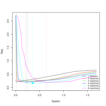
(a) Model 5, uncorrelated design.

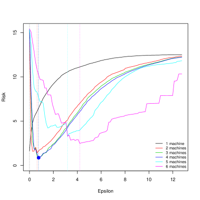
(b) Model 5, correlated design.

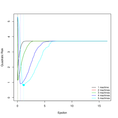
(c) Model 9.

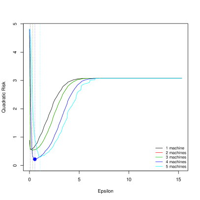
(d) Model 12.

Figure 3 (SM): Boxplots of quadratic errors, uncorrelated design. From left to right: lars, ridge, fnn, tree, randomForest, COBRA.

(a) Model 1.

(b) Model 2.

(c) Model 3.

(d) Model 4.

(e) Model 5.

(f) Model 6.

(g) Model 7.

(h) Model 8.

Figure 4 (SM): Boxplots of quadratic errors, correlated design. From left to right: lars, ridge, fnn, tree, randomForest, COBRA.

(a) Model 1.

(b) Model 2.

(c) Model 3.

(d) Model 4.

(e) Model 5.

(f) Model 6.

(g) Model 7.

(h) Model 8.

Figure 5 (SM): Prediction over the testing set, uncorrelated design. The more points on the first bissectrix, the better the prediction.

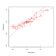
(a) Model 1.

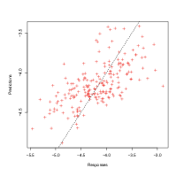
(b) Model 2.

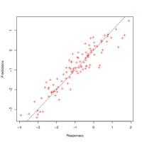
(c) Model 3.

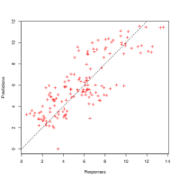
(d) Model 4.

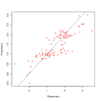
(e) Model 5.

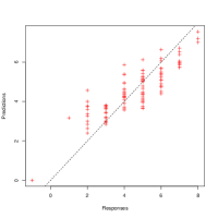
(f) Model 6.

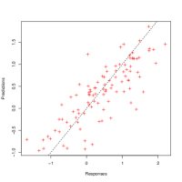
(g) Model 7.

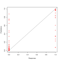
(h) Model 8.

Figure 6 (SM): Prediction over the testing set, correlated design. The more points on the first bissectrix, the better the prediction.

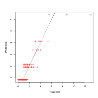
(a) Model 1.

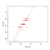
(b) Model 2.

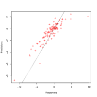
(c) Model 3.

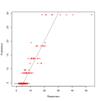
(d) Model 4.

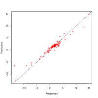
(e) Model 5.

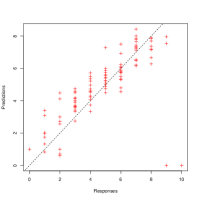
(f) Model 6.

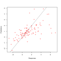
(g) Model 7.

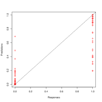
(h) Model 8.

Figure 7 (SM): Examples of reconstruction of the functional dependencies, for covariates $1$ to $4$.

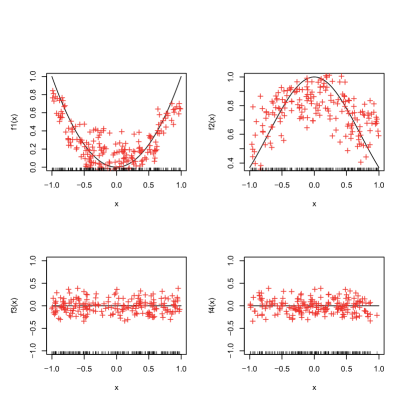
(a) Model 1, uncorrelated design.

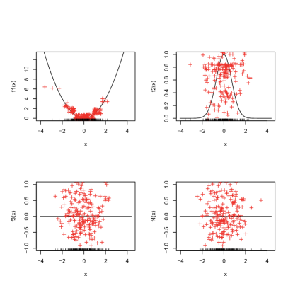
(b) Model 1, correlated design.

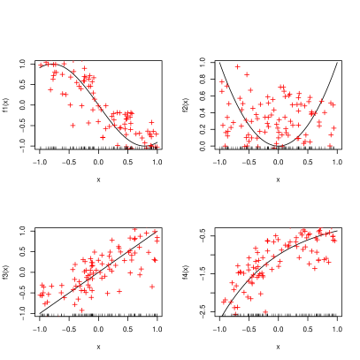
(c) Model 3, uncorrelated design.

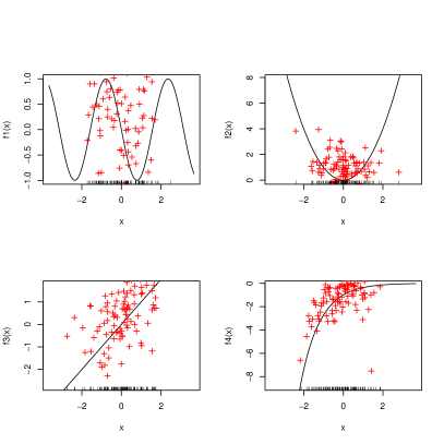
(d) Model 3, correlated design.

Figure 8 (SM): Boxplot of errors, high-dimensional models.

(a) Model 9

(b) Model 10

(c) Model 11

Figure 9 (SM): How stable is COBRA?

(a) Boxplot of errors: Initial sample is randomly cut ($1000$ replications of Model 12).

(b) Empirical risk with respect to the size of subsample $\mathcal{D}_{k}$, in Model 12.

Figure 10 (SM): Boxplot of errors: EWA vs COBRA

(a) Model 9.

(b) Model 10.

(c) Model 11.

(d) Model 12.

Figure 11 (SM): Prediction over the testing set, real-life data sets.

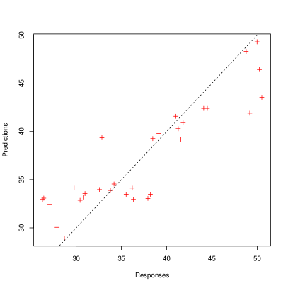
(a) Concrete Slump Test.

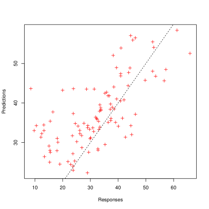
(b) Concrete Compressive Strength.

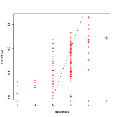
(c) Wine Quality, red wine.

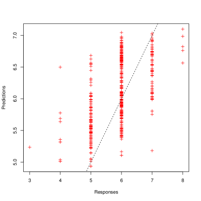
(d) Wine Quality, white wine.

Figure 12 (SM): Boxplot of quadratic errors, real-life data sets.

(a) Concrete Slump Test.

(b) Concrete Compressive Strength.

(c) Wine Quality, red wine.

(d) Wine Quality, white wine.

References

- Aneiros and Vieu (2014) Aneiros, G., Vieu, P., 2014. Variable selection in infinite-dimensional problems. Statistics & Probability Letters 94, 12–20.
- Biau (2012) Biau, G., 2012. Analysis of a random forests model. Journal of Machine Learning Research 13, 1063–1095.
- Bongiorno et al. (2014) Bongiorno, E.G., Salinelli, E., Goia, A., Vieu, P., 2014. Contributions in infinite-dimensional statistics and related topics. Società Editrice Esculapio.
- Cholaquidis et al. (2015) Cholaquidis, A., Fraiman, R., Kalemkerian, J., Llop, P., 2015. An nonlinear aggregation type classifier. Preprint.
- Cortez et al. (2009) Cortez, P., Cerdeira, A., Almeida, F., Matos, T., Reis, J., 2009. Modeling wine preferences by data mining from physicochemical properties. Decision Support Systems 47, 547–553.
- Cule (2012) Cule, E., 2012. ridge: Ridge Regression with automatic selection of the penalty parameter. URL: http://CRAN.R-project.org/package=ridge. r package version 2.1-2.
- Devroye et al. (1996) Devroye, L., Györfi, L., Lugosi, G., 1996. A Probabilistic Theory of Pattern Recognition. Springer.
- Ferraty and Vieu (2006) Ferraty, F., Vieu, P., 2006. Nonparametric Functional Data Analysis: Theory and Practice. Springer.
- Giraud (2014) Giraud, C., 2014. Introduction to High-Dimensional Statistics. Chapman & Hall/CRC.
- Goia and Vieu (2014) Goia, A., Vieu, P., 2014. A partitioned single functional index model. Computational Statistics .
- Guedj (2013) Guedj, B., 2013. COBRA: COmBined Regression Alternative. URL: http://cran.r-project.org/web/packages/COBRA/index.html. r package version 0.99.4.
- Györfi et al. (2002) Györfi, L., Kohler, M., Krzyżak, A., Walk, H., 2002. A Distribution-Free Theory of Nonparametric Regression. Springer.
- Hastie and Efron (2012) Hastie, T., Efron, B., 2012. lars: Least Angle Regression, Lasso and Forward Stagewise. URL: http://CRAN.R-project.org/package=lars. r package version 1.1.
- Knaus (2010) Knaus, J., 2010. snowfall: Easier cluster computing (based on snow). URL: http://CRAN.R-project.org/package=snowfall. r package version 1.84.
- van der Laan et al. (2007) van der Laan, M.J., Polley, E.C., Hubbard, A.E., 2007. Super learner. Statistical Applications in Genetics and Molecular Biology 6. doi:10.2202/1544-6115.1309.
- Li (2013) Li, S., 2013. FNN: Fast Nearest Neighbor search algorithms and applications. URL: http://CRAN.R-project.org/package=FNN. r package version 1.1.
- Liaw and Wiener (2002) Liaw, A., Wiener, M., 2002. Classification and regression by randomforest. R News 2, 18–22. URL: http://CRAN.R-project.org/doc/Rnews/.
- Malley et al. (2012) Malley, J.D., Kruppa, J., Dasgupta, A., Malley, K.G., Ziegler, A., 2012. Probability machines: Consistent probability estimation using nonparametric learning machines. Methods of Information in Medicine 51, 74–81. doi:10.3414/ME00-01-0052.
- Meier et al. (2009) Meier, L., van de Geer, S.A., Bühlmann, P., 2009. High-dimensional additive modeling. The Annals of Statistics 37, 3779–3821. doi:10.1214/09-AOS692.
- Mojirsheibani (1999) Mojirsheibani, M., 1999. Combining classifiers via discretization. Journal of the American Statistical Association 94, 600–609.
- Pekalska and Duin (2005) Pekalska, E., Duin, R.P.W., 2005. The Dissimilarity Representation for Pattern Recognition: Foundations and Applications. volume 64 of Machine Perception and Artificial Intelligence. World Scientific.
- Polley and van der Laan (2010) Polley, E.C., van der Laan, M.J., 2010. Super Learner in Prediction. Technical Report. UC Berkeley.
- Polley and van der Laan (2012) Polley, E.C., van der Laan, M.J., 2012. SuperLearner: Super Learner Prediction. URL: http://CRAN.R-project.org/package=SuperLearner. r package version 2.0-9.
- R Core Team (2014) R Core Team, 2014. R: A Language and Environment for Statistical Computing. R Foundation for Statistical Computing. Vienna, Austria. URL: http://www.R-project.org/.
- Ripley (2012) Ripley, B., 2012. tree: Classification and regression trees. URL: http://CRAN.R-project.org/package=tree. r package version 1.0-32.
- Yeh (1998) Yeh, I.C., 1998. Modeling of strength of high performance concrete using artificial neural networks. Cement and Concrete Research 28, 1797–1808.
- Yeh (2007) Yeh, I.C., 2007. Modeling slump flow of concrete using second-order regressions and artificial neural networks. Cement and Concrete Composites 29, 474–480.