Analysis of the radiative $\Lambda_{b}\rightarrow\Lambda\gamma$ transition in SM and scenarios with one or two universal extra dimensions

We investigate the radiative process of the $\Lambda_{b}\rightarrow\Lambda\gamma$ in the standard model as well as models with one or two compact universal extra dimensions. Using the form factors entered to the low energy matrix elements, calculated via light cone QCD in full theory, we calculate the total decay width and branching ratio of this decay channel. We compare the results of the extra dimensional models with those of the standard model on the considered physical quantities and look for the deviations of the results from the standard model predictions at different values of the compactification scale ($1/R$).

PACS number(s): 12.60.-i, 13.30.-a, 13.30.Ce, 14.20.Mr

1 Introduction

As it is well-known, the flavor changing neutral current (FCNC) transitions are prominent tools to indirectly search for the new physics (NP) effects. There are many mesonic and baryonic processes based on the $b\rightarrow s$ transition at quark level investigated in the literature via different NP models and compared the obtained results with the experimental data to put constraints on the NP parameters. One of the most important channels in agenda of different experimental groups is the baryonic FCNC $\Lambda_{b}\rightarrow\Lambda\ell^{+}\ell^{-}$ decay channel. The CDF Collaboration at Fermilab reported the first observation on this mode at muon channel [1]. The measured branching ratio is comparable with the SM prediction [2] within the errors of form factors. Comparing the different NP models’ predictions with the experimental data on this channel, it is possible to obtain information about and put limits on the parameters of the models. In our previous work, we put a lower limit to the compactification parameter of the universal extra dimension (UED) via this channel comparing the theoretical calculations with the experimental data [3].

The LHCb experiment at the LHC has been taking data for proton-proton collision in 2011 and 2012 at $\sqrt{s}=7$ and $8$ TeV, respectively, integrating a luminosity in excess of $3fb^{-1}$ [4, 5]. The LHCb measurement on the differential branching ratio of the $\Lambda_{b}\rightarrow\Lambda\mu^{+}\mu^{-}$ is in its final stage [6]. Considering these experimental progresses and the accessed luminosity we hope we will able to study more decay channels such as the radiative baryonic decay of $\Lambda_{b}\rightarrow\Lambda\gamma$ at LHCb [6, 4, 5, 7]. In this connection, we study this radiative decay channel in SM as well as UED with a single ED (UED5) and two EDs (UED6) in the present work. There are many works dedicated to the analysis of different decay channels in UED5 in the literature (for some of them see [3, 8, 9, 10, 11, 12, 13, 14, 15, 16, 17, 18, 19, 20, 21, 22, 23]). However, the number of works devoted to the applications of the UED6 is relatively few. As the expression of the only Wilson coefficient $C^{eff}_{7}$ now is available in UED6 [24], it is possible to study the radiative channels based on the $b\rightarrow s\gamma$.

In [25], the UED6 is employed to analyze the $B\to K\eta^{(\prime)}\gamma$ decay channel, where by comparing the results with the experimental data, a lower limit of $400$ GeV is put for the compactification scale. For some other previous constraints on the compactification factor obtained via electroweak precision tests, some cosmological constraints and different hadronic channels in UED5 see for instance [3, 29, 26, 11, 30, 28, 27]. We shall use the latest lower limits on the compactification factor $1/R$ obtained from different FCNC transitions in UED5 model [31], some FCNC transitions in UED6 model [25], electroweak precision tests [29], cosmological constraints [32], direct searches [33] as well as the latest results of the Higgs search at the LHC and of the electroweak precision data for the S and T parameters [34].

Scenarios with EDs play crucial roles among models beyond the SM. The main feature that leads to the difference among ED models is the number of dimensions added to the SM. In the UED5, we have an extra universal compactified dimension compared to the SM, while in UED6 we consider two extra UEDs. Because of the universality, the SM particles can propagate into the UEDs and interact with the Kaluza-Klein (KK) modes existing in EDs. As a result of these interactions, the new Feynman diagrams appear and this leads to a modification in the Wilson coefficients entered the low energy Hamiltonians defining the hadronic decay channels [35, 36, 10, 24]. In the UED5, the ED is compactified to the orbifold $S^{1}/Z_{2}$, with the fifth coordinate $x_{5}=y$ changing from $0$ to $2\pi R$. The points $y=0$ and $y=\pi R$ are fixed points of this orbifold. The boundary conditions at these points give the KK mode expansion of the fields. The masses of the KK particles in this model are obtained in terms of compactification scale as ${m_{n}}^{2}={m_{0}}^{2}+n^{2}/R^{2}$ where $n=1,2,...$ and $m_{0}$ represents the zeroth mode mass referring to the SM particles (for more about the model see [10, 27, 28, 37, 38, 39, 40, 41, 42]).

Models with two EDs are more attractive since they reply to some questions existing in the SM [43]. In this model, cancellations of chiral anomalies allow the existence of the right-handed neutrinos and predict the correct number of the fermion families [43, 44, 45]. At the same time, this model provides a natural explanation for the long lifetime of the proton [46, 47]. In UED6 models also, all the SM fields are assumed to propagate into both flat EDs that are already compactified on a chiral square of the side $L=\pi R$ [43, 48, 24]. The KK particles existing in this model are marked by two positive integers $k$ and $l$ which symbolize quantization of momentum along the EDs. The masses of these particles are given in terms of the compactification scale by $M_{(k,l)}=\sqrt{k^{2}+l^{2}}/R$ [43]. In this model, particles on first KK level with KK numbers ($1,0$) are odd under KK parity. These particles may be produced only in pairs at colliders. The particles on level-$2$ are even under KK parity and have KK numbers ($1,1$) [48]. This may lead to a totally different sets of signatures involving the resonances of the heavy top and bottom quarks [48, 49]. The masses of particles on level-2 are $\sqrt{2}$ factor larger than the masses of particles on level-1 [43]. This makes the particles at level -2 be most easily accessible at LHC [49]. For more details about the UED6 model and some of its applications see for instance [24, 43, 45, 46, 47, 49].

The outline of the article is as follows. In next section, we present the effective Hamiltonian responsible for the $\Lambda_{b}\rightarrow\Lambda\gamma$ in SM, UED5 and UED6 as well as the transition matrix elements in terms of form factors. In section 3, we calculate the decay width and branching ratio of the decay under consideration and numerically analyze them. In this section, we also compare the results of UED5 and UED6 with the SM predictions and look for the deviations from the SM at different values of the compactification radius.

2 The radiative $\Lambda_{b}\rightarrow\Lambda\gamma$ transition in SM, UED5 and UED6 models

In the present section, we present the effective Hamiltonian and show how the Wilson coefficient $C^{eff}_{7}$ changes both in UED scenarios with one and two extra dimensions compared to the SM. We also define the transition matrix elements appeared in the amplitude of the considered decay in terms of form factors.

2.1 The effective Hamiltonian

At quark level, the general effective Hamiltonian for $b\rightarrow s\gamma$ and $b\rightarrow sg$ transitions in SM and in terms of Wilson coefficients and operators is given by [35]

$${\cal H}^{eff} = -\frac{G_{F}}{\sqrt{2}}V_{tb}V_{ts}^{\ast}\bigg{[}{\sum\limits_{i=1}^{6}}C_{i}({\mu})Q_{i}({\mu})+C_{7\gamma}(\mu)Q_{7\gamma}(\mu)+C_{8G}(\mu)Q_{8G}(\mu)\bigg{]},$$ (2.1)

where $G_{F}$ is the Fermi weak coupling constant and $V_{ij}$ are elements of the Cabibbo-Kobayashi-Maskawa (CKM) mixing matrix. The complete list of the operators entered to the above Hamiltonian is given as

$$Q_{1}~{}\!\!\! = \!\!\!({\bar{s}}_{\alpha}c_{\beta})_{V-A}({\bar{c}}_{\beta}b_{\alpha})_{V-A},~{}$$

$$Q_{2}~{}\!\!\! = \!\!\!({\bar{s}}_{\alpha}c_{\alpha})_{V-A}({\bar{c}}_{\beta}b_{\beta})_{V-A},~{}$$

$$Q_{3}~{}\!\!\! = \!\!\!({\bar{s}}_{\alpha}b_{\alpha})_{V-A}\sum\limits_{q}({\bar{q}}_{\beta}q_{\beta})_{V-A},~{}$$

$$Q_{4}~{}\!\!\! = \!\!\!({\bar{s}}_{\beta}b_{\alpha})_{V-A}\sum\limits_{q}({\bar{q}}_{\alpha}q_{\beta})_{V-A},~{}$$

$$Q_{5}~{}\!\!\! = \!\!\!({\bar{s}}_{\alpha}b_{\alpha})_{V-A}\sum\limits_{q}({\bar{q}}_{\beta}q_{\beta})_{V+A},~{}$$

$$Q_{6}~{}\!\!\! = \!\!\!({\bar{s}}_{\beta}b_{\alpha})_{V-A}\sum\limits_{q}({\bar{q}}_{\alpha}q_{\beta})_{V+A},~{}$$

$$Q_{7\gamma}\!\!\! = \!\!\!{e\over 4\pi^{2}}\bar{s}_{\alpha}\sigma^{\mu\nu}(m_{b}R+m_{s}L)b_{\alpha}\,F_{\mu\nu},~{}$$

$$Q_{8G}\!\!\! = \!\!\!{g_{s}\over 4\pi^{2}}\bar{s}_{\alpha}\sigma^{\mu\nu}(m_{b}R+m_{s}L)T^{a}_{\alpha\beta}b_{\beta}\,G^{a}_{\mu\nu},~{}$$ (2.2)

where $Q_{1,2}$, $Q_{3,4,5,6}$ and $Q_{7\gamma,8G}$ are the current-current (tree), QCD penguin and the magnetic penguin operators, respectively. $\alpha$ and $\beta$ are the color indices, $R=(1+\gamma_{5})/2$ is the right-handed projector and $L=(1-\gamma_{5})/2$ is the left-handed projector. In the above operators $e$ and $g_{s}$ are the coupling constants of the electromagnetic and strong interactions, respectively. $F_{\mu\nu}$ is the field strength tensor of the electromagnetic field and is defined by

$$F_{\mu\nu}(x) = -i(\varepsilon_{\mu}q_{\nu}-\varepsilon_{\nu}q_{\mu})e^{iqx}~{},$$ (2.3)

where $\varepsilon_{\mu}$ is the polarization vector of the photon and $q$ is its momentum. The most relevant contribution to $b\rightarrow s\gamma$ comes from the magnetic penguin operator $Q_{7\gamma}$. Hence the effective Hamiltonian in our case can be written as,

$${\cal H}^{eff}(b\rightarrow s\gamma) = -{G_{F}e\over 4\pi^{2}\sqrt{2}}V_{tb}V_{ts}^{\ast}C^{eff}_{7}(\mu)\bar{s}\sigma_{\mu\nu}\Big{[}m_{b}R+m_{s}L\Big{]}bF^{\mu\nu}~{},$$ (2.4)

where $C^{eff}_{7}$ is relevant the Wilson coefficient. Under scenarios with EDs including one or two compact extra dimensions, the form of effective Hamiltonian remains unchanged, but the Wilson coefficient $C^{eff}_{7}$ is modified because of additional Feynman diagrams coming from the interactions of the KK particles with themselves as well as the SM particles in the bulk. This coefficient in SM is given as [50]

$$C_{7}^{eff}(\mu_{b})\!\!\! = \!\!\!\eta^{\frac{16}{23}}C_{7}(\mu_{W})+\frac{8}{3}\left(\eta^{\frac{14}{23}}-\eta^{\frac{16}{23}}\right)C_{8}(\mu_{W})+C_{2}(\mu_{W})\sum_{i=1}^{8}h_{i}\eta^{a_{i}}~{},$$

where

$$\eta\!\!\! = \!\!\!\frac{\alpha_{s}(\mu_{W})}{\alpha_{s}(\mu_{b})}~{},$$ (2.6)

and

$$\alpha_{s}(x)=\frac{\alpha_{s}(m_{Z})}{1-\beta_{0}\frac{\alpha_{s}(m_{Z})}{2\pi}\ln(\frac{m_{Z}}{x})}.$$ (2.7)

Here $\alpha_{s}(m_{Z})=0.118$ and $\beta_{0}=\frac{23}{3}$. The values of coefficients $a_{i}$ and $h_{i}$ in Eq.(2.1) are given as

$$\frac{}{}\begin{array}[]{rrrrrrrrrl}a_{i}=(\!\!&\frac{14}{23},&\frac{16}{23},&\frac{6}{23},&-\frac{12}{23},&0.4086,&-0.4230,&-0.8994,&0.1456&\!\!)\vspace{0.1cm},\\ h_{i}=(\!\!&2.2996,&-1.0880,&-\frac{3}{7},&-\frac{1}{14},&-0.6494,&-0.0380,&-0.0186,&-0.0057&\!\!).\end{array}$$ (2.8)

Also $C_{2}(\mu_{W})$, $C_{7}(\mu_{W})$ and $C_{8}(\mu_{W})$ in Eq.(2.1) are defined in the following way:

$$C_{2}(\mu_{W})=1~{},~{}~{}C_{7}(\mu_{W})=-\frac{1}{2}D^{\prime}_{0}(x_{t})~{},~{}~{}C_{8}(\mu_{W})=-\frac{1}{2}E^{\prime}_{0}(x_{t})~{},$$ (2.9)

where $D^{\prime}_{0}(x_{t})$ and $E^{\prime}_{0}(x_{t})$ are expressed as

$$D^{\prime}_{0}(x_{t})\!\!\! = \!\!\!-\frac{(8x_{t}^{3}+5x_{t}^{2}-7x_{t})}{12(1-x_{t})^{3}}+\frac{x_{t}^{2}(2-3x_{t})}{2(1-x_{t})^{4}}\ln x_{t}~{},$$ (2.10)

$$E^{\prime}_{0}(x_{t})\!\!\! = \!\!\!-\frac{x_{t}(x_{t}^{2}-5x_{t}-2)}{4(1-x_{t})^{3}}+\frac{3x_{t}^{2}}{2(1-x_{t})^{4}}\ln x_{t}~{}.$$ (2.11)

The Wilson coefficient $C^{eff}_{7}$ in UED5 has been calculated in [35, 9, 10, 51, 52, 50]. In this model, each periodic function $F(x_{t},1/R)$ ($F=$ $D^{\prime}$ or $E^{\prime}$) inside the Wilson coefficient includes a SM part $F_{0}(x_{t})$ plus an additional part in terms of compactification factor $1/R$ due to new interactions, i.e.,

$$F(x_{t},1/R)=F_{0}(x_{t})+\sum_{n=1}^{\infty}F_{n}(x_{t},x_{n}),$$ (2.12)

where $x_{t}=\frac{m_{t}^{2}}{m_{W}^{2}}$, $x_{n}=\displaystyle{m_{n}^{2}\over m_{W}^{2}}$, and $m_{n}=\displaystyle{n\over R}$. Here $m_{t}$, $m_{W}$ and $m_{n}$ are masses of the top quark, $W$ boson and KK particles (non-zero modes), respectively. In UED5, the functions $D^{\prime}(x_{t},1/R)$ and $E^{\prime}(x_{t},1/R)$ in terms of compactification parameter $1/R$ are given as

$$D^{\prime}(x_{t},1/R)=D^{\prime}_{0}(x_{t})+\sum_{n=1}^{\infty}D^{\prime}_{n}(x_{t},x_{n}),~{}~{}~{}~{}~{}E^{\prime}(x_{t},1/R)=E^{\prime}_{0}(x_{t})+\sum_{n=1}^{\infty}E^{\prime}_{n}(x_{t},x_{n})~{},$$ (2.13)

where the functions including KK contributions are written as

$$\sum_{n=1}^{\infty}D^{\prime}_{n}(x_{t},x_{n})\!\!\! = \!\!\!\frac{x_{t}[37-x_{t}(44+17x_{t})]}{72(x_{t}-1)^{3}}$$

$$+ \!\!\!\frac{\pi m_{W}R}{12}\Bigg{[}\int_{0}^{1}dy\,(2y^{1/2}+7y^{3/2}+3y^{5/2})\,\coth(\pi m_{W}R\sqrt{y})$$

$$- \!\!\!\frac{x_{t}(2-3x_{t})(1+3x_{t})}{(x_{t}-1)^{4}}J(R,-1/2)$$

$$- \!\!\!\frac{1}{(x_{t}-1)^{4}}\{x_{t}(1+3x_{t})+(2-3x_{t})[1-(10-x_{t})x_{t}]\}J(R,1/2)$$

$$- \!\!\!\frac{1}{(x_{t}-1)^{4}}[(2-3x_{t})(3+x_{t})+1-(10-x_{t})x_{t}]J(R,3/2)$$

$$- \!\!\!\frac{(3+x_{t})}{(x_{t}-1)^{4}}J(R,5/2)\Bigg{]}~{},$$

and

$$\sum_{n=1}^{\infty}E^{\prime}_{n}(x_{t},x_{n})\!\!\! = \!\!\!\frac{x_{t}[17+(8-x_{t})x_{t}]}{24(x_{t}-1)^{3}}$$ (2.15)

$$+ \!\!\!\frac{\pi m_{W}R}{4}\Bigg{[}\int_{0}^{1}dy\,(y^{1/2}+2y^{3/2}-3y^{5/2})\,\coth(\pi m_{W}R\sqrt{y})$$

$$- \!\!\!{x_{t}(1+3x_{t})\over(x_{t}-1)^{4}}J(R,-1/2)$$

$$+ \!\!\!\frac{1}{(x_{t}-1)^{4}}[x_{t}(1+3x_{t})-1+(10-x_{t})x_{t}]J(R,1/2)$$

$$- \!\!\!\frac{1}{(x_{t}-1)^{4}}[(3+x_{t})-1+(10-x_{t})x_{t}]J(R,3/2)$$

$$+ \!\!\!{(3+x_{t})\over(x_{t}-1)^{4}}J(R,5/2)\Bigg{]}~{},$$

where

$$J(R,\alpha)=\int_{0}^{1}dy\,y^{\alpha}\left[\coth(\pi m_{W}R\sqrt{y})-x_{t}^{1+\alpha}\coth(\pi m_{t}R\sqrt{y})\right]~{}.$$ (2.16)

The Wilson coefficient $C_{7}^{eff}(1/R)$ in the UED6 model with two extra dimensions is given by [24]

$$C^{\rm eff}_{i}(\mu)=C^{\rm eff}_{i\,{\rm SM}}(\mu)+\Delta C^{\rm eff}_{i}(\mu)\,,\quad i=1,\ldots,8$$ (2.17)

where

$$\Delta C^{\rm eff}_{i}(\mu)=\sum_{n=0}^{\infty}\left(\frac{\alpha_{s}}{4\pi}\right)^{n}\Delta C_{i}^{{\rm eff}(n)}(\mu)\,,$$ (2.18)

and

$$\Delta C_{i}^{{\rm eff}(0)}(\mu_{0})=\begin{cases}\phantom{-}0&\mbox{for $i=1,\ldots,6$,}\\[4.30554pt] -\frac{1}{2}{\sum\limits_{k,l}}^{\prime}A^{(0)}(x_{kl})&\mbox{for $i=7$,}\\[8.61108pt] -\frac{1}{2}{\sum\limits_{k,l}}^{\prime}F^{(0)}(x_{kl})&\mbox{for $i=8$.}\end{cases}$$ (2.19)

The superscript (^′) in summation means that the KK sums run only over the restricted ranges $k\geq 1$ and $l\geq 0$, i.e., $\sum_{k,l}^{\prime}=\sum_{k\geq 1}\sum_{l\geq 0}$. The upper limits for $k$ and $l$ are restricted as $k+l\leq N_{KK}$ where $N_{KK}$ can get values in the interval $(5-15)$ [24]. The parameter $N_{KK}$ in our calculations is the total number of contributing KK modes [28]. The highest KK level in this compactification is fixed by $N_{KK}=\Lambda R$ [53], where $\Lambda$ is a scale at which the QCD interactions become strong in the ultraviolet [49]. In the case of UED5 $N_{KK}=n$, however, as the KK sums over $n$ up to infinity is convergent we have no dependence on the $N_{KK}$ after the KK sums. In the case of UED6 the KK mode sums diverge in the limit $N_{KK}\rightarrow\infty$ because the KK spectrum is denser than the UED5 case. The electroweak observables convergence in four and five dimensions at one loop, become logarithmically divergent at $d=6$ and more divergent in higher dimensions [28]. Hence we should put a cut-off and, as a result, an upper limit to $k+l$.

The Inami-Lim functions inside the $C_{7}^{eff}$ in leading order are decomposed as

$$X^{(0)}(x_{kl}) =\sum\limits_{I={\scriptstyle W},a,H}X^{(0)}_{I}(x_{kl})\,,\quad X=A,F\,$$ (2.20)

where $x_{kl}$ is defined as

$$x_{kl}=(k^{2}+l^{2})/(R^{2}m_{W}^{2}),$$ (2.21)

and the functions $X^{(0)}_{W,a,H}(x_{kl})$ define the contributions because of the exchange of KK modes which would be the Goldstone bosons $G^{\pm}_{(kl)}$, $W$-bosons $W^{\pm}_{\mu(kl)}$ and the scalar fields $a^{\pm}_{(kl)}$ as well as $W^{\pm}_{H(kl)}$. They are given as

$$A_{W}^{(0)}(x_{kl}) = \frac{x_{t}(6((x_{t}-3)x_{t}+3)x_{kl}^{2}-3(5(x_{t}-3)x_{t}+6)x_{kl}+x_{t}(8x_{t}+5)-7)}{12(x_{t}-1)^{3}}$$

$$+ \frac{1}{2}(x_{kl}-2)x_{kl}^{2}\ln\left(\frac{x_{kl}}{x_{kl}+1}\right)-\frac{(x_{kl}+x_{t})^{2}(x_{kl}+3x_{t}-2)}{2(x_{t}-1)^{4}}\ln\left(\frac{x_{kl}+x_{t}}{x_{kl}+1}\right)~{},$$

$$F_{W}^{(0)}(x_{kl}) = \frac{x_{t}\left(-6((x_{t}-3)x_{t}+3)x_{kl}^{2}-3((x_{t}-3)x_{t}+6)x_{kl}+(x_{t}-5)x_{t}-2\right)}{4(x_{t}-1)^{3}}$$

$$- \frac{3}{2}(x_{kl}+1)x_{kl}^{2}\ln\left(\frac{x_{kl}}{x_{kl}+1}\right)+\frac{3(x_{kl}+1)(x_{kl}+x_{t})^{2}}{2(x_{t}-1)^{4}}\ln\left(\frac{x_{kl}+x_{t}}{x_{kl}+1}\right)~{},$$

$$A_{a}^{(0)}(x_{kl}) = \frac{x_{t}\left(6x_{kl}^{2}-3(x_{t}(2x_{t}-9)+3)x_{kl}+(29-7x_{t})x_{t}-16\right)}{36(x_{t}-1)^{3}}$$

$$- \frac{(x_{kl}+3x_{t}-2)(x_{t}+x_{kl}((x_{kl}-x_{t}+4)x_{t}-1))}{6(x_{t}-1)^{4}}\ln\left(\frac{x_{kl}+x_{t}}{x_{kl}+1}\right)$$

$$- \frac{1}{6}(x_{kl}-2)x_{kl}\ln\left(\frac{x_{kl}}{x_{kl}+1}\right)~{},$$

$$F_{a}^{(0)}(x_{kl}) = \frac{x_{t}\left(-6x_{kl}^{2}+\left(6x_{t}^{2}-9x_{t}-9\right)x_{kl}+(7-2x_{t})x_{t}-11\right)}{12(x_{t}-1)^{3}}$$

$$+ \frac{(x_{kl}+1)(x_{t}+x_{kl}((x_{kl}-x_{t}+4)x_{t}-1))}{2(x_{t}-1)^{4}}\ln\left(\frac{x_{kl}+x_{t}}{x_{kl}+1}\right)$$

$$+ \frac{1}{2}x_{kl}(x_{kl}+1)\ln\left(\frac{x_{kl}}{x_{kl}+1}\right)~{},$$

$$A_{H}^{(0)}(x_{kl}) = \frac{x_{t}\left(6\left(x_{t}^{2}-3x_{t}+3\right)x_{kl}^{2}-3\left(3x_{t}^{2}-9x_{t}+2\right)x_{kl}-7x_{t}^{2}+29x_{t}-16\right)}{36(x_{t}-1)^{3}}$$

$$- \frac{(x_{kl}+1)\left(x_{kl}^{2}+(4x_{t}-2)x_{kl}+x_{t}(3x_{t}-2)\right)}{6(x_{t}-1)^{4}}\ln\left(\frac{x_{kl}+x_{t}}{x_{kl}+1}\right)$$

$$+ \frac{1}{6}x_{kl}\left(x_{kl}^{2}-x_{kl}-2\right)\ln\left(\frac{x_{kl}}{x_{kl}+1}\right)~{},$$

and

$$F_{H}^{(0)}(x_{kl}) = -\frac{x_{t}\left(6\left(x_{t}^{2}-3x_{t}+3\right)x_{kl}^{2}+3\left(3x_{t}^{2}-9x_{t}+10\right)x_{kl}+2x_{t}^{2}-7x_{t}+11\right)}{12(x_{t}-1)^{3}}$$

$$- \frac{1}{2}x_{kl}(x_{kl}+1)^{2}\ln\left(\frac{x_{kl}}{x_{kl}+1}\right)+\frac{(x_{kl}+x_{t})(x_{kl}+1)^{2}}{2(x_{t}-1)^{4}}\ln\left(\frac{x_{kl}+x_{t}}{x_{kl}+1}\right)~{}.$$

2.2 Transition amplitude and matrix elements

The amplitude for this transition is obtained by sandwiching the effective Hamiltonian between the final and initial baryonic states

$${\cal M}^{(\Lambda_{b}\rightarrow\Lambda\gamma)} = \langle\Lambda(p_{\Lambda})|{\cal H}^{eff}|\Lambda_{b}(p_{\Lambda_{b}})\rangle~{},$$ (2.28)

where $p_{\Lambda}$ and $p_{\Lambda_{b}}$ are momenta of the $\Lambda$ and $\Lambda_{b}$ baryons, respectively. In order to proceed, we need to define the following transition matrix elements in terms of two form factors $f_{2}^{T}$ and $g_{2}^{T}$:

$$\langle\Lambda(p_{\Lambda})|\bar{s}\;\sigma_{\mu\nu}q^{\nu}(g_{V} + \gamma_{5}g_{A})b|\Lambda_{b}(p_{\Lambda_{b}})\rangle$$ (2.29)

$$= \bar{u}_{\Lambda}(p_{\Lambda})\sigma_{\mu\nu}q^{\nu}\Big{(}g_{V}f_{2}^{T}(0)+\gamma_{5}g_{A}g_{2}^{T}(0)\Big{)}u_{\Lambda_{b}}(p_{\Lambda_{b}}),$$

where $g_{V}=1+m_{s}/m_{b}$, $g_{A}=1-m_{s}/m_{b}$, and $\bar{u}_{\Lambda}$ and $u_{\Lambda_{b}}$ are spinors of the $\Lambda$ and $\Lambda_{b}$ baryons, respectively. In the following, we will use the values of the form factors calculated via light cone QCD sum rules in full theory [2].

3 Decay width and branching ratio

In this section we would like to calculate the total decay width and branching ratio of the transition under consideration. Using the aforesaid transition matrix elements in terms of form factors, we find the $1/R$-dependent total decay width in terms of the two form factors as

$$\Gamma_{(\Lambda_{b}\rightarrow\Lambda\gamma)}(1/R)=\frac{G_{F}^{2}\alpha_{em}|V_{tb}V_{ts}^{*}|^{2}m_{b}^{2}}{64\pi^{4}}|C_{7}^{eff}(1/R)|^{2}\left(\frac{m_{\Lambda_{b}}^{2}-m_{\Lambda}^{2}}{m_{\Lambda_{b}}}\right)^{3}\Big{(}g_{V}^{2}|f_{2}^{T}(0)|^{2}+g_{A}^{2}|g_{2}^{T}(0)|^{2}\Big{)},$$

where $\alpha_{em}$ is the fine structure constant at Z mass scale. In order to calculate the $1/R$-dependent branching ratio, we need to multiply the total decay width by the lifetime of the initial baryon $\Lambda_{b}$ and divide by $\hbar$. To numerically analyze the obtained results, we use some input parameters as presented in Table 1. For the quark masses, we use the $\overline{MS}$ scheme values [54] (see Table 2).

Input Parameters	Values
$m_{W}$	$80.38$ $GeV$
$m_{\Lambda_{b}}$	$5.619$ $GeV$
$m_{\Lambda}$	$1.1156$ $GeV$
$\mu_{b}$	$5$ $GeV$
$\mu_{W}$	$80.4$ $GeV$
$\mu_{0}$	$160$ $GeV$
$\tau_{\Lambda_{b}}$	$1.425\times 10^{-12}$ $s$
$\hbar$	$6.582\times 10^{-25}GeVs$
$G_{F}$	$1.17\times 10^{-5}$ $GeV^{-2}$
$\alpha_{em}$	$1/137$
$|V_{tb}V_{ts}^{*}|$	$0.041$

Table 1: The values of some input parameters, mainly taken from PDG [54], ​​used in the numerical analysis.

Quarks	masses in $\overline{MS}$ scheme
$m_{s}$	$(0.095\pm 0.005)$ $GeV$
$m_{b}$	$(4.18\pm 0.03)$ $GeV$
$m_{t}$	$160^{+4.8}_{-4.3}$ $GeV$

Table 2: The values of quark masses in $\overline{MS}$ scheme [54].

As we previously mentioned, we use the values of form factors calculated via light cone QCD sum rules in full theory as the main inputs in numerical analysis [2]. Their values are presented in Table 3.

	form factors at $q^{2}=0$
$f_{2}^{T}(0)$	$0.295\pm 0.105$
$g_{2}^{T}(0)$	$0.294\pm 0.105$

Table 3: The values of form factors $f^{T}_{2}(0)$ and $g^{T}_{2}(0)$ [2].

In this part we present the numerical values of the Wilson coefficient $C^{eff}_{7}$ obtained from the previously presented formulas in SM, UED5 and UED6 models. In SM, its value is obtained as $C^{eff}_{7}=-0.295$. We depict the values of the Wilson coefficient $C^{eff}_{7}$ at different values of $1/R$ in UED5 and UED6 scenarios with $N_{KK}=(5,10,15)$ in Table 4.

$1/R$	$C^{eff}_{7}$	$C^{eff}_{7}$	$C^{eff}_{7}$	$C^{eff}_{7}$
[GeV]	(UED5)	(UED6 for $N_{KK}=5$)	(UED6 for $N_{KK}=10$)	(UED6 for $N_{KK}=15$)
$200$	$-0.198$	$-0.053$	$0.048$	$0.110$
$400$	$-0.265$	$-0.224$	$-0.198$	$-0.182$
$600$	$-0.281$	$-0.262$	$-0.250$	$-0.243$
$800$	$-0.287$	$-0.276$	$-0.269$	$-0.265$
$1000$	$-0.289$	$-0.283$	$-0.278$	$-0.279$

Table 4: The numerical values of Wilson coefficient $C^{eff}_{7}$ at the different values of $1/R$ in UED5 and UED6 for $N_{KK}=(5,10,15)$.

Making use of all given input values we find the value of the branching ratio in SM as presented in Table 5. For comparison, we also give the results of other related works [55, 56, 57, 58, 59, 60] in the same Table as well as the upper limit from PDG [54]. From this Table we see that, within the errors, our result is consistent with those of QCD sum rules [56, 57] and CZ current [59] and exactly the same with pole model’s prediction [60]. However, our prediction differs considerably from these of light cone QCD sum rules [55], covariant oscillator quark model (COQM) [58] and Ioffe current [59]. The difference between our SM prediction on the branching ratio with that of [55] with the same method can be attributed to the point that in [55] the authors consider the distribution amplitudes (DAs) of $\Lambda$ baryon as the main inputs of the light cone QCD sum rule method up to twist 6, however, in our case the form factors have been calculated considering the DAs up to twist 8. Besides, in [55] the higher conformal spin contributions to the DAs are not taken into account, while the calculations of form factors in our case include these contributions. Finally, in [55] the form factors are calculated in heavy quark effective limit while we use form factors calculated in full QCD without any approximation. The order of branching ratio shows that this channel can be accessible at LHCb.

Ref.	BR($\Lambda_{b}\rightarrow\Lambda\gamma$)
Our result	$(1.003-4.457)\times 10^{-5}$
Light-cone sum rule [55]	$(0.63-0.73)\times 10^{-5}$
Three-point QCD sum rule [56]	$(3.1\pm 0.6)\times 10^{-5}$
QCD sum rule [57]	$(3.7\pm 0.5)\times 10^{-5}$
COQM [58]	$0.23\times 10^{-5}$
CZ current [59]	($1.99^{+0.34}_{-0.31}$)$\times 10^{-5}$
Ioffe current [59]	($0.61^{+0.14}_{-0.13}$)$\times 10^{-6}$
Pole Model [60]	$(1.0-4.5)\times 10^{-5}$
PDG [54]	$<1.3\times 10^{-3}$ ($CL=90\%)$

Table 5: The values of branching ratio in SM.

In order to look for the differences between the predictions of the SM and the considered UED scenarios, we present the dependence of the central values of the branching ratio on $1/R$ at different models in figure 1. Note that to better see the deviations between the SM predictions and those of UED scenarios, in all figures, we plot the branching ratio in terms of $1/R$ in the interval $200~{}GeV\leq 1/R\leq 2000~{}GeV$. However we will consider the latest lower limits on the compactification factor obtained from different approaches in our analysis and discussions. The latest lower limits on $1/R$ are: $400~{}GeV$ put by some FCNC transitions in UED6 model [25], $500~{}GeV$ put via cosmological constraints [32], $600~{}GeV$ obtained via different FCNC transitions in UED5 model (for instance see [31]) and electroweak precision tests [29], $1.41~{}TeV$ quoted via direct searches at ATLAS Collaboration [33] as well as $650~{}(850\sim 1350)~{}GeV$ from the latest results of the Higgs search/discovery at the LHC for UED5 (UED6) [34] and $700~{}(900\sim 1500)~{}GeV$ from the electroweak precision data for S and T parameters in the case of UED5 (UED6) [34].

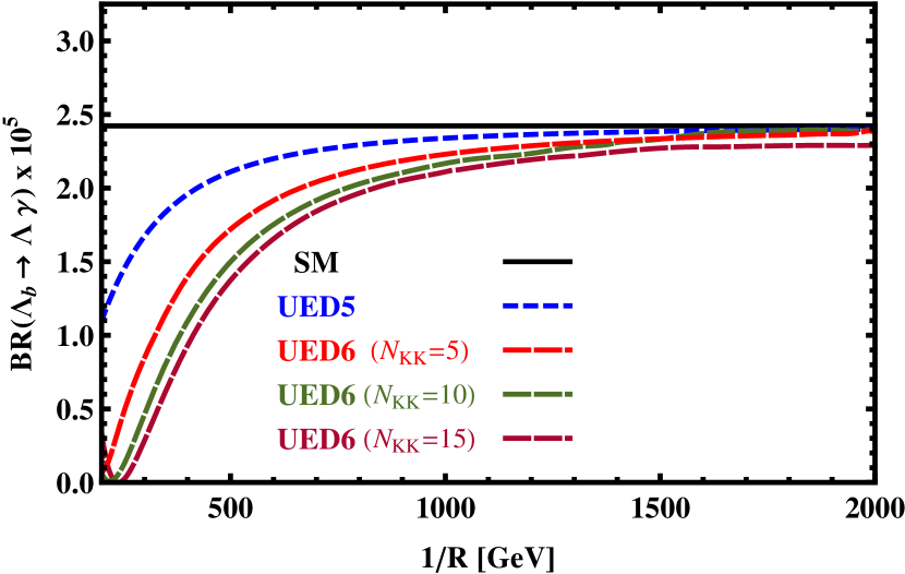
Figure 1: The dependence of branching ratio for $\Lambda_{b}\rightarrow\Lambda\gamma$ decay channel on compactification factor $1/R$ in SM, UED5 and UED6 models with $N_{KK}=(5,10,15)$ when the central values of the form factors are used.

From figure 1 we see that there are distinctive differences between the SM predictions and those of UED models, especially UED6 for $N_{KK}=15$, at small values of the compactification factor $1/R$. These differences exist in the lower limits obtained by different FCNC transitions in UED5 and UED6, cosmological constraints, electroweak precision tests [25, 32, 31, 29] and the latest results of the Higgs search at the LHC and of the electroweak precision data for the S and T parameters [34], however, they become small when $1/R$ approaches to $1~{}TeV$. Our analysis show that the UED scenarios give close results to the SM for $1/R\geq 1~{}TeV$. Hence, when considering the lower limit $1.41~{}TeV$ quoted via direct searches at ATLAS Collaboration [33] we see very small deviations of the UED models predictions from those of the SM for the decay channel under consideration.

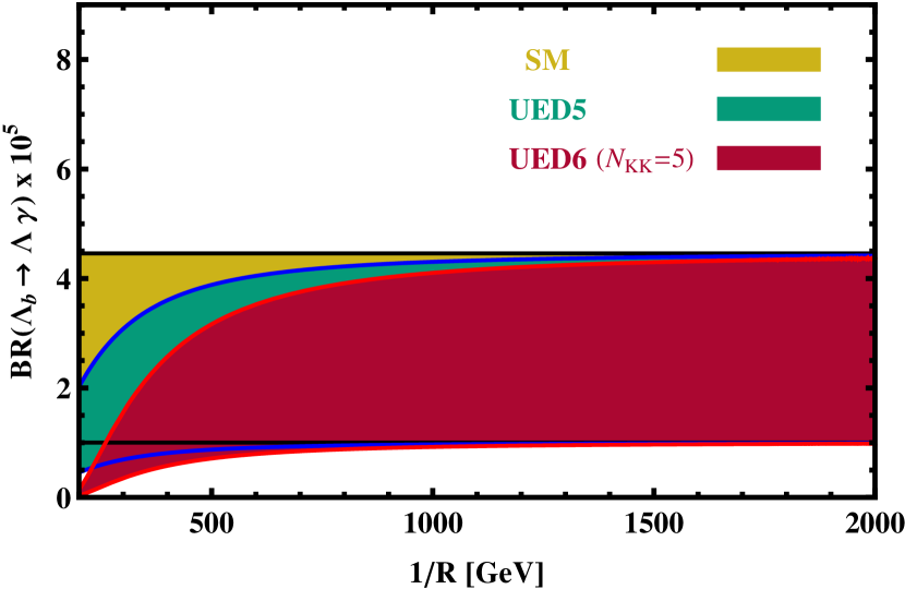
Figure 2: The dependence of branching ratio on compactification factor $1/R$ for $\Lambda_{b}\rightarrow\Lambda\gamma$ decay in SM, UED5 and UED6 with $N_{KK}=5$ when the uncertainties of the form factors are considered.

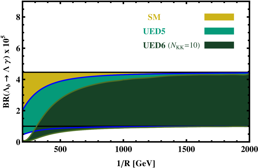
Figure 3: The same as figure 2 but for $N_{KK}=10$.

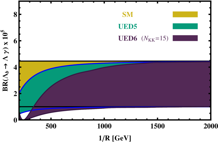
Figure 4: The same as figure 2 but for $N_{KK}=15$.

At the end of this section, we present the dependence of the branching ratio on $1/R$ considering the errors of form factors in figures 2, 3 and 4. From these figures we read that the errors of form factors can not totally kill the differences between the predictions of the UED models on the branching ratio of $\Lambda_{b}\rightarrow\Lambda\gamma$ channel with that of the SM at lower values of the compactification scale. These discrepancies can also be seen in the lower limits favored by different FCNC transitions in UED5 and UED6 models, cosmological constraints, electroweak precision tests [25, 32, 31, 29] as well as the latest results of the Higgs search/discovery at the LHC and of the electroweak precision data for the S and T parameters [34] for UED5. However, when $1/R$ approaches to $1~{}TeV$ all differences of the UED results with the SM predictions are roughly killed and there are no considerable deviations of the UED predictions from that of the SM at $1.41~{}TeV$ quoted via direct searches at ATLAS Collaboration [33] for the $\Lambda_{b}\rightarrow\Lambda\gamma$ decay channel.

4 Conclusion

In the present work, we have performed a comprehensive analysis of the $\Lambda_{b}\rightarrow\Lambda\gamma$ decay channel in the SM, UED5 and UED6 scenarios. In particular, we calculated the total decay rate and branching ratio for this channel in different UED scenarios and looked for the deviations of the results from the SM predictions. We used the expression of the Wilson coefficient $C^{eff}_{7}$ entered to the low energy effective Hamiltonian calculated in SM, UED5 and UED6 models. We also used the numerical values of the form factors calculated via light cone QCD sum rules in full theory as the main inputs of the numerical analysis. We detected considerable discrepancies between the considered UED models’ predictions with that of the SM prediction at lower values of the compactification factor. These discrepancies can not totally be killed by the uncertainties of the form factors at lower values of $1/R$ and they exist at the lower limits favored by different FCNC transitions in UED5 and UED6 models, cosmological constraints, electroweak precision tests [25, 32, 31, 29] as well as the latest results of the Higgs search/discovery at the LHC and of the electroweak precision data for the S and T parameters [34]. However, when $1/R$ approaches to $1~{}TeV$ all deviations of the UED results from the SM predictions are roughly killed and there are no considerable deviations of the UED predictions for the $\Lambda_{b}\rightarrow\Lambda\gamma$ decay channel from that of the SM at $1.41~{}TeV$ quoted via direct searches at ATLAS Collaboration [33]. The order of branching ratio for $\Lambda_{b}\rightarrow\Lambda\gamma$ decay channel in SM shows that this channel can be accessible at LHCb.

Note Added: After completing this work, a related study titled as “Bounds on the compactification scale of two universal extra dimensions from exclusive $b\to s\gamma$ decays” was submitted to arXiv on 28 Feb 2013 with arXiv:1302.7240 [hep-ph] [61], where a similar analysis is done only in UED6 using the form factors calculated from the heavy quark effective theory and average value of the $N_{KK}$. When we compare our results with those of [61], we see that there is a considerable difference between our result on the branching ratio of the decay under consideration in SM with those of [61]. Although the central values of the branching ratios in two works obtained via UED6 have similar behaviors, the bands of UED6 in our case sweep wide ranges compared to those of [61]. Especially, the band of UED6 ($N_{KK}=10$) in [61] starts to completely cover the SM band at $1/R\approx 800~{}GeV$, while in our case, we see a similar behavior at $1/R\approx 1000~{}GeV$. These small differences can be attributed to different form factors used in the numerical analysis as well as other input parameters.

5 Acknowledgement

We would like to thank A. Freitas and U. Haisch for useful discussions.

References

• [1] T. Aaltonen et al. [ CDF Collaboration ], “Observation of the Baryonic Flavor-Changing Neutral Current Decay $\Lambda_{b}^{0}\to\Lambda\mu^{+}\mu^{-}$”, Phys. Rev. Lett. 107, 201802 (2011) [arXiv:1107.3753 [hep-ex]].
• [2] T. M. Aliev, K. Azizi, M. Savci, “Analysis of the $\Lambda_{b}\rightarrow\Lambda\ell^{+}\ell^{-}$ decay in QCD”, Phys. Rev. D 81, 056006 (2010) [arXiv:1001.0227 [hep-ph]].
• [3] K. Azizi, S. Kartal, N. Katirci, A. T. Olgun, Z. Tavukoglu, “Constraint on compactification scale via recently observed baryonic $\Lambda_{b}\rightarrow\Lambda\ell^{+}\ell^{-}$ channel and analysis of the $\Sigma_{b}\rightarrow\Sigma\ell^{+}\ell^{-}$ transition in SM and UED scenario”, JHEP 1205, 024 (2012) [arXiv:1203.4356 [hep-ph]].
• [4] C. Bozzi, “LHCb Results on Semileptonic $B$/$B_{s}$/$\Lambda_{b}$ Decays”, (2013) [arXiv:1303.4219 [hep-ex]].
• [5] LHCb Collaboration (M.-H. Schune for the collaboration), “Future prospects at LHCb”, LHCB-PROC 005 (2013) [arXiv:1301.4811 [hep-ex]].
• [6] Our personal communications with Michal Kreps from LHCb Collaboration.
• [7] G. Mancinelli, “Rare Decays With LHCb”, Conference: C12-07-15.2 [arXiv:1212.4609 [hep-ex]].
• [8] K. Azizi, N. Katirci, “Investigation of the $\Lambda_{b}\rightarrow\Lambda\ell^{+}\ell^{-}$ transition in universal extra dimension using form factors from full QCD”, JHEP 1101, 087 (2011) [arXiv:1011.5647 [hep-ph]].
• [9] A. J. Buras, M. Spranger, A. Weiler, “The impact of universal extra dimensions on the unitarity triangle and rare K and B decays”, Nucl. Phys. B 660, 225 (2003) [arXiv:hep-ph/0212143].
• [10] A. J. Buras, A. Poschenrieder, M. Spranger, A. Weiler, “The Impact of Universal Extra Dimensions on $B\to X_{s}\gamma$, $B\to X_{s}g$, $B\to X_{s}\mu^{+}\mu^{-}$, $K_{L}\to\pi^{0}e^{+}e^{-}$, and $\varepsilon^{\prime}/\varepsilon$”, Nucl. Phys. B 678, 455 (2004) [arXiv:hep-ph/0306158].
• [11] P. Colangelo, F. De Fazio, R. Ferrandes, T. N. Pham, “Exclusive $B\to K^{(*)}\ell^{+}\ell^{-}$, $B\to K^{(*)}\nu{\bar{\nu}}$ and $B\to K^{*}\gamma$ transitions in a scenario with a single Universal Extra Dimension”, Phys. Rev. D 73, 115006 (2006) [arXiv:hep-ph/0604029].
• [12] V. Bashiry, K. Azizi, “Systematic analysis of the $B_{s}\rightarrow f_{0}\ell^{+}\ell^{-}$ in the universal extra dimension”, JHEP 1202, 021 (2012) [arXiv:1112.5243 [hep-ph]].
• [13] N. Katirci, K. Azizi, “B to strange tensor meson transition in a model with one universal extra dimension”, JHEP 1107, 043 (2011) [arXiv:1105.3636 [hep-ph]].
• [14] V. Bashiry, M. Bayar, K. Azizi, “Double-lepton polarization asymmetries and polarized forward backward asymmetries in the rare $b\rightarrow s\ell^{+}\ell^{-}$ decays in a single universal extra dimension scenario”, Phys. Rev. D 78, 035010 (2008) [arXiv:0808.1807 [hep-ph]].
• [15] Y.-M. Wang, M. J. Aslam, C.-D. Lü, “Rare decays of $\Lambda_{b}\rightarrow\Lambda\gamma$ and $\Lambda_{b}\rightarrow\Lambda\ell^{+}\ell^{-}$ in universal extra dimension model”, Eur. Phys. J. C 59, 847 (2009) [arXiv:0810.0609 [hep-ph]].
• [16] T. M. Aliev, M. Savcı, “$\Lambda_{b}\rightarrow\Lambda l^{+}l^{-}$ decay in universal extra dimensions”, Eur. Phys. J. C 50, 91 (2007) [arXiv:hep-ph/0606225].
• [17] F. De Fazio, “Rare B decays in a single Universal Extra Dimension scenario”, Nucl. Phys. Proc. Suppl. 174, 185 (2007) [arXiv:hep-ph/0610208].
• [18] B. B. Sirvanli, K. Azizi, Y. Ipekoglu, “Double-lepton polarization asymmetries and branching ratio in $B\rightarrow K_{0}^{*}(1430)l^{+}l^{-}$ transition from universal extra dimension model”, JHEP 1101, 069 (2011) [arXiv:1011.1469[hep-ph]].
• [19] K. Azizi, N. K. Pak, B. B. Sirvanli, “Double-Lepton Polarization Asymmetries and Branching Ratio of the $B\rightarrow\gamma l^{+}l^{-}$ transition in Universal Extra Dimension”, JHEP 1202, 034 (2012) [arXiv:1112.2927 [hep-ph]].
• [20] T. M. Aliev, M. Savci, B. B. Sirvanli, “Double-lepton polarization asymmetries in $\Lambda_{b}\rightarrow\Lambda l^{+}l^{-}$ decay in universal extra dimension model”, Eur. Phys. J. C 52, 375 (2007) [arXiv:hep-ph/0608143].
• [21] I. Ahmed, M. A. Paracha, M. J. Aslam, “Exclusive $B\rightarrow K_{1}l^{+}l^{-}$ decay in model with single universal extra dimension”, Eur. Phys. J. C 54, 591 (2008) [arXiv:0802.0740 [hep-ph]].
• [22] P. Colangelo, F. De Fazio, R. Ferrandes, T. N. Pham, “Spin effects in rare $B\to X_{s}\tau^{+}\tau^{-}$ and $B\to K^{(*)}\tau^{+}\tau^{-}$ decays in a single universal extra dimension scenario”, Phys. Rev. D 74, 115006 (2006) [arXiv:hep-ph/0610044].
• [23] R. Mohanta, A. K. Giri, “Study of FCNC-mediated rare $B_{s}$ decays in a single universal extra dimension scenario”, Phys. Rev. D 75, 035008 (2007) [arXiv:hep-ph/0611068].
• [24] A. Freitas, U. Haisch, “$B\rightarrow\chi_{s}\gamma$ in two universal extra dimensions”, Phys. Rev. D 77, 093008 (2008) [arXiv:0801.4346 [hep-ph]].
• [25] P. Biancofiore, P. Colangelo, F. D. Fazio, “$B\to K\eta^{(\prime)}\gamma$ decays in the standard model and in scenarios with universal extra dimensions”, Phys. Rev. D 85, 094012 (2012) [arXiv:1202.2289 [hep-ph]].
• [26] J. A. R. Cembranos, J. L. Feng, L. E. Strigari, “Exotic collider signals from the complete phase diagram of minimal universal extra dimensions”, Phys. Rev. D 75, 036004 (2007) [arXiv:hep-ph/0612157].
• [27] T. Appelquist, H.-U. Yee, “Universal Extra Dimensions and the Higgs Boson Mass”, Phys. Rev. D 67, 055002 (2003) [arXiv:hep-ph/0211023].
• [28] T. Appelquist, H. C. Cheng, B. A. Dobrescu, “Bounds on universal extra dimensions”, Phys. Rev. D 64, 035002 (2001) [arXiv:hep-ph/0012100].
• [29] I. Gogoladze, C. Macesanu, “Precision electroweak constraints on universal extra dimensions revisited”, Phys. Rev. D 74, 093012 (2006) [arXiv:hep-ph/0605207].
• [30] K. Agashe, N. G. Deshpande, G.-H. Wu, “Universal Extra Dimensions and $b\rightarrow s\gamma$”, Phys. Lett. B 514, 309 (2001) [arXiv:hep-ph/0105084].
• [31] U. Haisch, A. Weiler, “Bound on minimal universal extra dimensions from ${\bar{B}}\rightarrow X_{s}\gamma$”, Phys. Rev. D 76, 034014 (2007) [arXiv:hep-ph/0703064].
• [32] G. Belanger, M. Kakizaki, A. Pukhov, “Dark matter in UED: the role of the second KK level”, JCAP 1102, 009 (2011) [arXiv:1012.2577 [hep-ph]].
• [33] ATLAS Collaboration, “Search for Diphoton Events with Large Missing Transverse Momentum in $7~{}TeV$ pp Collision Data with the ATLAS Detector”, ATLAS-CONF-2012-072 (2012).
• [34] T. Kakuda, K. Nishiwaki, Kin-ya Oda, N. Okuda, R. Watanabe “Phenomenological constraints on universal extra dimensions at LHC and electroweak precision test” [ arXiv:1304.6362 [hep-ph]]; T. Kakuda, K. Nishiwaki, Kin-ya Oda, R. Watanabe, “Universal Extra Dimensions after Higgs Discovery” [arXiv:1305.1686 [hep-ph]].
• [35] G. Buchalla, A. J. Buras, M. E. Lautenbacher, “Weak Decays Beyond Leading Logarithms”, Rev. Mod. Phys. 68, 1125 (1996) [arXiv:hep-ph/9512380].
• [36] A. J. Buras, L. Merlo, E. Stamou, “The Impact of Flavour Changing Neutral Gauge Bosons on $B\rightarrow X_{s}\gamma$”, JHEP 1108, 124 (2011) [arXiv:1105.5146 [hep-ph]].
• [37] I. Antoniadis, “A possible new dimension at a few TeV”, Phys. Lett. B 246, 377 (1990).
• [38] I. Antoniadis, N. Arkani-Hamed, S. Dimopoulos and G. Dvali, “New dimensions at a millimeter to a fermi and superstrings at a TeV”, Phys. Lett. B 436, 257 (1998) [arXiv:hep-ph/9804398].
• [39] N. Arkani-Hamed, S. Dimopoulos and G. Dvali, “The hierarchy problem and new dimensions at a millimeter”, Phys. Lett. B 429, 263 (1998) [arXiv:hep-ph/9803315].
• [40] N. Arkani-Hamed, S. Dimopoulos and G. Dvali, “Phenomenology, astrophysics, and cosmology of theories with submillimeter dimensions and TeV scale quantum gravity”, Phys. Rev. D 59, 086004 (1999) [arXiv:hep-ph/9807344].
• [41] L. Randall, R. Sundrum, “An Alternative to Compactification”, Phys. Rev. Lett. 83, 4690 (1999) [arXiv:hep-th/9906064].
• [42] L. Randall, R. Sundrum, “Large Mass Hierarchy from a Small Extra Dimension”, Phys. Rev. Lett. 83, 3370 (1999) [arXiv:hep-ph/9905221].
• [43] A. Freitas, K. Kong, “Two universal extra dimensions and spinless photons at the ILC”, JHEP 0802, 068 (2008) [arXiv:0711.4124 [hep-ph]].
• [44] B. A. Dobrescu, E. Poppitz, “Number of Fermion Generations Derived from Anomaly Cancellation”, Phys. Rev. Lett. 87, 031801 (2001) [arXiv:hep-ph/0102010].
• [45] G. Burdman, “Two Universal Extra Dimensions”, AIP Conf. Proc. 903, 447 (2007) [arXiv:hep-ph/0611064].
• [46] K. Ghosh, A. Datta, “Phenomenology of spinless adjoints in two Universal Extra Dimensions”, Nucl. Phys. B 800, 109 (2008) [arXiv:0801.0943 [hep-ph]].
• [47] T. Appelquist, B. A. Dobrescu, E. Ponton, H.-U. Yee , “Proton Stability in Six Dimensions”, Phys. Rev. Lett. 87, 181802 (2001) [arXiv:hep-ph/0107056].
• [48] B. A. Dobrescu, K. Kong, R. Mahbubani, “Leptons and photons at the LHC: cascades through spinless adjoints”, JHEP 0707, 006 (2007) [arXiv:hep-ph/0703231].
• [49] G. Burdman, B. A. Dobrescu, Eduardo Ponton, “Resonances from Two Universal Extra Dimensions”, Phys. Rev. D 74, 075008 (2006) [arXiv:hep-ph/0601186].
• [50] A. Buras, M. Misiak, M. Münz, S. Pokorski, “Theoretical Uncertainties and Phenomenological Aspects of $B\rightarrow X_{s}\gamma$ Decay”, Nucl. Phys. B 424, 374 (1994) [arXiv:hep-ph/9311345].
• [51] M. Misiak, “The $b\rightarrow se^{+}e^{-}$ and $b\rightarrow s\gamma$ decays with next-to-leading logarithmic QCD-corrections”, Nucl. Phys. B 393, 23 (1993); Erratum-ibid B 439, 161 (1995).
• [52] B. Buras, M. Munz, “Effective Hamiltonian for $B\rightarrow X_{s}e^{+}e^{-}$ Beyond Leading Logarithms in the NDR and HV Schemes”, Phys. Rev. D 52, 186 (1995) [arXiv:hep-ph/9501281].
• [53] R. S. Chivukula, D. A. Dicus, H.-J. He, S. Nandi, “Unitarity of the Higher Dimensional Standard Model”, Phys. Lett. B 562, 109 (2003) [arXiv:hep-ph/0302263].
• [54] J. Beringer et al. (Particle Data Group), Phys. Rev. D 86, 010001 (2012).
• [55] Y.-M. Wang, Y. Li, C.-D. Lü , “Rare decays of $\Lambda_{b}\rightarrow\Lambda\gamma$ and $\Lambda_{b}\rightarrow\Lambda\ell^{+}\ell^{-}$ in the light cone sum rules”, Eur. Phys. J. C 59, 861 (2009).
• [56] P. Colangelo, F. De Fazio, R. Ferrandes, T.N. Pham, “FCNC $B_{s}$ and $\Lambda_{b}$ transitions: Standard Model versus a single Universal Extra Dimension scenario”, Phys. Rev. D 77, 055019 (2008) [arXiv:0709.2817 [hep-ph]].
• [57] C.-S. Huang, H.-G. Yan , “Exclusive Rare Decays of Heavy Baryons to Light Baryons: $\Lambda_{b}\rightarrow\Lambda\gamma$ and $\Lambda_{b}\rightarrow\Lambda\ell^{+}\ell^{-}$”, Phys. Rev. D 59, 114022 (1999), Erratum-ibid. D 61, 039901 (2000) [arXiv:hep-ph/9811303].
• [58] R. Mohanta, A. K. Giri, M. P. Khanna , M. Ishida, S. Ishida, “Weak Radiative Decay $\Lambda_{b}\rightarrow\Lambda\gamma$ and Quark-Confined Effects in the Covariant Oscillator Quark Model”, Prog. Theor. Phys. 102, 645 (1999) [arXiv:hep-ph/9908291].
• [59] L.-F. Gan, Y.-L. Liu, W.-B. Chen, M.-Q. Huang, “Improved Light-cone QCD Sum Rule Analysis Of The Rare Decays $\Lambda_{b}\rightarrow\Lambda\gamma$ And $\Lambda_{b}\rightarrow\Lambda\ell^{+}\ell^{-}$”, Commun. Theor. Phys. 58, 872 (2012) [arXiv:1212.4671 [hep-ph]].
• [60] T. Mannel, S. Recksiegel, “Flavour Changing Neutral Current Decays of Heavy Baryons: The Case $\Lambda_{b}\rightarrow\Lambda\gamma$”, J. Phys. G 24, 979 (1998) [ arXiv:hep-ph/9701399]
• [61] P. Biancofiore, “Bounds on the compactification scale of two universal extra dimensions from exclusive $b\to s\gamma$ decays”, (2013) [arXiv:1302.7240 [hep-ph]].