Unified Description of Dirac Electrons on a Curved Surface of Topological Insulators

Abstract

Existence of a protected surface state described by a massless Dirac equation is a defining property of the topological insulator. Though this statement can be explicitly verified on an idealized flat surface, it remains to be addressed to what extent it could be general. On a curved surface, the surface Dirac equation is modified by the spin connection terms. Here, in the light of the differential geometry, we give a general framework for constructing the surface Dirac equation starting from the Hamiltonian for bulk topological insulators. The obtained unified description clarifies the physical meaning of the spin connection.

1 Introduction

Low-energy electron states on the surface of a topological insulator is protected by the time reversal symmetry, which is encoded as (a nontrivial value of) the $\mathbb{Z}_{2}$ topological index. [1, 2, 3] Electrons in these surface states obey a massless Dirac equation, and possess a linear energy dispersion forming a gapless conic structure, i.e., a Dirac cone in the reciprocal space. Such a conic dispersion has been observed experimentally by angle-resolved photoemission spectroscopy measurements. [4, 5, 6, 7, 8]

The existence of a single Dirac cone on an ideally flat large cleaved surface of a three-dimensional (3D), strong topological insulator is thus incontrovertible, [9] while it is less clear how the low-energy electrons behave on curved surfaces. [10, 11, 12] Realistic surfaces of the topological insulator have imperfections, such as terraces and islands, [13, 14] that have been also experimentally observed. [15] Samples of a finite volume have a closed surface as a whole, or a set of facets. The corner of two facets are sometimes better described as a curved single surface. [13] In addition to such natural occurrence, the role of the curvature becomes particularly important in artificially fabricated topological insulator nanostructures such as nanowires [16] and nanoparticles. [17]

The behavior of low-energy electrons has been studied theoretically, on a curved surface of e.g., cylindrical [11, 12, 18, 19, 20, 21] or spherical [10, 22, 17] form. In case of the cylindrical geometry, a remarkable feature is the appearance of a finite-size energy gap separating the upper and lower Dirac cones of surface electron states. In refs. zhang1,zhang2,egger,bardarson,imura1,imura3, the origin of this gap has been much discussed; the opening of the gap was attributed to half-odd integral quantization of the orbital angular momentum ($L_{z}$ in a cylinder pointed to the $z$-axis). The quantization is half-shifted by what is often called the “Berry’s phase $\pi$”. Most schematically, this interpretation may be sketched as follows: first, the real spin of a surface electron is constrained onto the tangential plane at any point on a curved surface; this feature is often referred to as “spin-to-surface locking”. As a consequence of this locking, when the electron goes around the cylinder, the surface curvature induces “spin connection” [23] that sums up to the Berry’s phase $\pi$.

In spite of the accumulation of such studies, we have so far not reached the unified description of the low-energy electrons on curved surfaces. When existence of a protected surface state is suggested by the bulk-boundary correspondence, [24, 25] it is natural to expect that low-energy electron states are described by a Dirac-type equation even on curved surfaces, while an explicit demonstration of this has been lacking. Note that the bulk-boundary correspondence ensures on a flat surface the existence of a protected gapless surface state described by a massless Dirac Hamiltonian, while on curved surfaces one generally expects that such an effective surface Dirac Hamiltonian will be modified by spin connection terms.

Let us try to give a brief overview of the present status of theoretical studies dealing with a curved surface of topological insulators. This issue has been addressed mainly in cylindrical [11, 12, 18, 19, 20, 21] and spherical [10, 22, 17] systems by employing two different types of approaches, with the exception of refs. takane and imura4 that have treated the case of hyperbolic surfaces. The first group of studies is based on the two-dimensional (2D) Dirac equation for a flat surface, and takes account of the curved nature of the surface by a coordinate transformation. [10, 11, 12, 18, 19, 22] Certainly, the resulting curved surface Dirac theory can be applicable to an arbitrary curved surface in this approach, but for a clear reason that it assumes a 2D Dirac theory from the outset, it fails to answer the question whether the low-energy electrons obey indeed a Dirac-type equation. The drawback of this approach is that it ignores the 3D nature of the original problem. If one recalls the importance of bulk-boundary correspondence in the conceptual foundation of the topological insulator, it may not be surprising that such an approach turns out to keep only “half of the information”.

In the second group of approaches, on contrary, such a difficulty is well overcome. There, one starts from a 3D bulk Hamiltonian and derives an effective 2D theory for a given curved surface by the use of the $\bm{k}\cdot\bm{p}$ approximation. [20, 13, 17, 21, 26] By its construction such an approach takes well account of the 3D nature of the problem. In the remainder of this paper, we extend this type of analyses so as to describe the surface state of a topological insulator of an arbitrary shape. As a result, we are led to the unified description of such a surface state on arbitrary curved surfaces.

Construction of the general framework may also help to clarify the following issues related to the curved surface Dirac theory. One is on the origin of the Berry’s phase $\pi$ in the context of spin-to-surface locking. As already mentioned, the Berry’s phase $\pi$ is recognized as a consequence of $\pm 2\pi$ rotation of the real spin caused by the spin-to-surface locking. [11, 12, 18, 19, 20] This locking, however, breaks down, for example, in spherical topological insulators, [17] since any spin configurations under the complete spin-to-surface locking cannot satisfy the periodic boundary condition for the sphere without singularities. This fact raises a natural question: is the spin-to-surface locking essential in the appearance of the Berry’s phase $\pi$? Note here that a finite-size energy gap associated with the spin connection also appears in the spherical geometry. [10, 22, 17]

Another issue that will be addressed in the paper concerns the “physical” interpretation of the spin connection. The spin connection appears in the curved surface Dirac theory as a fictitious vector potential in the effective Hamiltonian. Though mathematically well-defined, encoding the information on the curved nature of the surface, its physical origin is somewhat mysterious, especially for those researchers in the condensed matter community. Here, in this paper we attempt an accessible presentation of this issue.

In the next section we introduce a set of curvilinear coordinates adapted for describing an arbitrary curved surface. In §3, we present a general framework to derive the effective surface Hamiltonian for the low-energy electrons within the $\bm{k}\cdot\bm{p}$ approximation. We show that the effective Hamiltonian is indeed expressed in a generalized Dirac form with the spin connection. The role of the spin connection is clarified and given an intuitive interpretation. In §4, we discuss the boundary condition for a spinor wave function in spatially periodic systems, and identify the precise origin of the Berry’s phase $\pi$. In §5, our framework is applied to two known examples, namely to the case of cylindrical and spherical geometries, to demonstrate how it works. The last section is devoted to summary and discussion. We set $\hbar=1$ throughout this paper.

2 Basic formulations

Before introducing a curved surface and a set of proper (curvilinear) coordinates for describing it, let us first specify what is in the bulk. We start with the following bulk effective Hamiltonian for a (3D, isotropic, strong) topological insulator in the continuum limit: [27, 28] $H_{\rm bulk}=m(\mib{p})\tau_{z}+A\tau_{x}(\mib{\sigma}\cdot\mib{p})$, where $\mib{p}=-{\rm i}\nabla$ and $m({\mib p})=m_{0}+m_{2}\mib{p}^{2}$ is the mass term. The two types of Pauli matrices $\mib{\sigma}=(\sigma_{x},\sigma_{y},\sigma_{z})$ and $\mib{\tau}=(\tau_{x},\tau_{y},\tau_{z})$ represent, respectively, the real and the orbital spin degrees of freedom. If the ordinary matrix representation of $\mib{\tau}$ is used, $H_{\rm bulk}$ is expressed as

$$H_{\rm bulk}=\left[\begin{array}[]{cc}m({\mib p})&A(\mib{\sigma}\cdot\mib{p})\\ A(\mib{\sigma}\cdot\mib{p})&-m({\mib p})\end{array}\right].$$ (3)

Throughout the paper we assume that mass parameters are chosen such that $m_{0}>0$ and $m_{2}<0$. When this is the case, the existence of a protected surface state is ensured by the bulk-boundary correspondence. On a flat surface, the surface state exhibits a gapless spectrum, described by a massless Dirac Hamiltonian. On a curved surface, the Dirac equation is modified by the spin connection terms, as we demonstrate below.

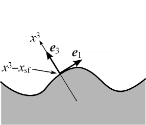
Figure 1: Curved surface of a 3D topological insulator: cross section in the plane spanned by ${\mib e}_{1}$ and ${\mib e}_{3}$.

Let us consider a curved surface of the sample described by two coordinates $(x^{1},x^{2})$ as $X^{\alpha}=f^{\alpha}(x^{1},x^{2})$, where $\mib{X}=(X^{1},X^{2},X^{3})$ represents the position of an arbitrary point on the surface in the 3D Cartesian coordinates (see Fig. 1). Depending on the geometry (e.g., closed vs. open surfaces, etc.), the coordinate $x_{i}$ represents either a linear (non-cyclic) or a cyclic coordinate. For simplicity we focus on samples whose entire surface is described by a single set of functions $\{f^{\alpha}\}$, although with little modification our argument can be extended to cases where the entire surface is wrapped by several patches and a separate set of functions is needed to describe each patch. We introduce a set of curvilinear coordinates suitable for analyzing low-energy electron states of the topological insulator localized in the vicinity of its surface. As surface electron states have a finite penetration depth $\lambda$, we require that the set of curvilinear coordinates are well-defined only in the surface region of width on the order of $\lambda$.

Let ${\mib e}_{1}$ and ${\mib e}_{2}$ be the two tangent vectors defined by

$${\mib e}_{i}=\frac{\partial\mib{X}}{\partial x^{i}}.$$ (4)

Note that ${\mib e}_{1}$ and ${\mib e}_{2}$ are not necessarily orthogonal with each other nor normalized to be unity. Let ${\mib e}_{3}$ be the unit normal vector defined by

$${\mib e}_{3}=\frac{{\mib e}_{1}\times{\mib e}_{2}}{|{\mib e}_{1}\times{\mib e}_{2}|},$$ (5)

which for simplicity is assumed to be outward normal to the surface. We introduce the third (perpendicular) coordinate $x^{3}$ along the straight line designated by ${\mib e}_{3}$, and set $x^{3}=x_{\rm sf}$ just on the surface. Let us consider fictitious internal surfaces obtained by varying $(x^{1},x^{2})$ at fixed values of $x^{3}$ satisfying $x_{\rm sf}\geq x^{3}\gtrsim x_{\rm sf}-\lambda$. These surfaces are well-defined over the entire sample as long as the smallest value of local radius of curvature at $x^{3}=x_{\rm sf}$ is much longer than $\lambda$. Let $f^{\alpha}(x^{1},x^{2},x^{3})$ be the function that describes the internal surface at $x^{3}$. In terms of this we define ${\mib e}_{1}$ and ${\mib e}_{2}$ similar to eq. (4). Now ${\mib e}_{1}$ and ${\mib e}_{2}$ become functions of $(x^{1},x^{2},x^{3})$, while ${\mib e}_{3}$ is independent of $x^{3}$. We employ $(x^{1},x^{2},x^{3})$ as the curvilinear coordinates with the basis vectors

$${\mib e}_{1} ={\mib e}_{1}(x^{1},x^{2},x^{3}),$$ (6)

$${\mib e}_{2} ={\mib e}_{2}(x^{1},x^{2},x^{3}),$$ (7)

$${\mib e}_{3} ={\mib e}_{3}(x^{1},x^{2}).$$ (8)

Let us introduce ${\mib e}^{i}$ that satisfies ${\mib e}_{i}\cdot{\mib e}^{j}=\delta_{ij}$. We also introduce the metric tensors in a symmetric bilinear form defined by $g_{ij}\equiv{\mib e}_{i}\cdot{\mib e}_{j}$ and $g^{ij}\equiv{\mib e}^{i}\cdot{\mib e}^{j}$, which satisfy $g_{ik}g^{kj}=\delta_{ij}$. Here and hereafter we use the convention that a repeated index, such as $i$, $j$, and $k$, should be summed over $1,2,3$. Obviously, $g_{33}=g^{33}=1$ as $|\mib{e}_{3}|=1$, and $g_{13}=g_{23}=g^{13}=g^{23}=0$ as ${\mib e}_{1}\bot{\mib e}_{3}$ and ${\mib e}_{2}\bot{\mib e}_{3}$. In this coordinate system, an infinitesimal volume element is given by ${\rm d}V={\rm d}S{\rm d}x^{3}$ with

$${\rm d}S=\sqrt{{\mathcal{G}}}{\rm d}x^{1}{\rm d}x^{2}$$ (9)

being an infinitesimal area element, where

$$\mathcal{G}(x^{1},x^{2},x^{3})\equiv{\rm det}\{g_{ij}\}=g_{11}g_{22}-g_{12}^{2}.$$ (10)

Within the curvilinear coordinates presented above, the 3D Cartesian coordinates $(X^{1},X^{2},X^{3})=(x,y,z)$ and the differential operators with respect to them are represented as $X^{\alpha}=e_{i\alpha}x^{i}$ and $\partial/\partial{X^{\alpha}}={e^{i}}_{\alpha}\partial_{i}$, where $\partial_{i}\equiv\partial/\partial{x^{i}}$. For later convenience we decompose the Laplacian into two parts as $\nabla^{2}=\Lambda_{\perp}+\Lambda_{\parallel}$, where

$$\Lambda_{\perp} =\frac{1}{\sqrt{\mathcal{G}}}\partial_{3}\left(\sqrt{\mathcal{G}}\partial_{3}\right),$$ (11)

$$\Lambda_{\parallel} =\sum_{i,j=1}^{2}\frac{1}{\sqrt{\mathcal{G}}}\partial_{i}\left(\sqrt{\mathcal{G}}g^{ij}\partial_{j}\right).$$ (12)

Finally we present a set of equations which describe the spatial variation of ${\mib e}_{i}$ against $x^{1}$ and $x^{2}$. The tangent vectors obey the Gauss equation,

$$\partial_{j}{\mib e}_{i}=\sum_{k=1}^{2}\Gamma_{ij}^{k}{\mib e}_{k}+b_{ij}{\mib e}_{3},$$ (13)

where

$$b_{ij} =-(\partial_{j}{\mib e}_{3})\cdot{\mib e}_{i},$$ (14)

$$\Gamma_{ij}^{k} =\frac{1}{2}g^{kl}\left(\partial_{j}g_{li}+\partial_{i}g_{lj}-\partial_{l}g_{ij}\right).$$ (15)

The unit normal vector obeys the Weingarten equation,

$$\partial_{j}{\mib e}_{3}=-\sum_{i=1}^{2}{b_{j}}^{i}{\mib e}_{i},$$ (16)

where

$${b_{j}}^{i}=\sum_{k=1}^{2}g^{ik}b_{kj}=-(\partial_{j}{\mib e}_{3})\cdot{\mib e}^{i}.$$ (17)

These equations are used in Appendices B and C in deriving, or simplifying, matrix elements of the effective Hamiltonian.

3 The effective Hamiltonian in a Dirac form

Let us now derive the effective Hamiltonian on the curved surface specified by the curvilinear coordinates $(x^{1},x^{2},x^{3})$. The derivation consists of four steps.

In the first step, we rewrite eq. (3) in terms of the curvilinear coordinates, and then divide it into components, either perpendicular or parallel to the local tangent of curved surface spanned by ${\mib e}_{1}$ and ${\mib e}_{2}$. The former describes penetration of the surface wave functions into the bulk, while the latter determines low-energy properties of the surface states. As a result, $H_{\rm bulk}$ is decomposed as $H_{\rm bulk}=H_{\perp}+H_{\parallel}$ with

$$H_{\perp} =\left[\begin{array}[]{cc}m_{0}-m_{2}\Lambda_{\perp}&-{\rm i}A\sigma^{3}\partial_{3}\\ -{\rm i}A\sigma^{3}\partial_{3}&-m_{0}+m_{2}\Lambda_{\perp}\end{array}\right],$$ (20)

$$H_{\parallel} =\left[\begin{array}[]{cc}-m_{2}\Lambda_{\parallel}&-{\rm i}A\sum_{i=1}^{2}\sigma^{i}\partial_{i}\\ -{\rm i}A\sum_{i=1}^{2}\sigma^{i}\partial_{i}&m_{2}\Lambda_{\parallel}\end{array}\right],$$ (23)

where we have used $\mib{\sigma}\cdot\nabla=\sigma^{i}\cdot\partial_{i}$ with

$$\sigma^{i}\equiv{\mib e}^{i}\cdot\mib{\sigma}.$$ (24)

In the second step, we solve the eigenvalue equation $H_{\perp}|\psi\rangle=E_{\perp}|\psi\rangle$, [27, 28, 20, 17] associated with the perpendicular part (20), to find the two basis eigenstates $|\pm\rangle$ for constructing the surface effective Hamiltonian. The appropriate boundary condition for $|\psi\rangle$ is $|\psi(x^{3}=x_{\rm sf})\rangle=\mib 0$. That is, all four components of the wave function $|\psi\rangle$ vanish on the surface at $x^{3}=x_{\rm sf}$. As the simplest approximation, we replace $\Lambda_{\perp}$ in $H_{\perp}$ with

$$\Lambda_{\perp} =\partial_{3}^{2}+\frac{1}{2}\langle\partial_{3}{\rm ln}{\mathcal{G}}\rangle\partial_{3}$$

$$\equiv\partial_{3}^{2}+\Delta(x^{1},x^{2})\partial_{3},$$ (25)

where the definition of the average $\langle\cdots\rangle$ over $x^{3}$ is given below [see eq. (47)]. Then, we can show that the eigenvalue equation has surface solutions of the damped form, $|\psi\rangle={\rm e}^{\kappa(x^{3}-x_{\rm ef})}|u\rangle$. Here $\kappa$ characterizing the penetration depth $\lambda$ is determined by ${\rm det}\{M_{\perp}\}=0$ with

$$M_{\perp}=\left[\begin{array}[]{cc}m_{0}-m_{2}\zeta-E_{\perp}&-{\rm i}A\kappa\sigma^{3}\\ -{\rm i}A\kappa\sigma^{3}&-m_{0}+m_{2}\zeta-E_{\perp}\end{array}\right],$$ (28)

where $\zeta=\kappa^{2}+\Delta\kappa$. Let us introduce the two eigenvectors $\mib{n}_{\pm}$ of $\sigma^{3}$. They satisfy

$$\sigma^{3}\mib{n}_{\pm}=\pm\mib{n}_{\pm},$$ (29)

and are regarded as local spin quantization axis. $\mib{n}_{\pm}$ points in the $\pm{\mib e}_{3}$ direction if the spin axes $(s_{x},s_{y},s_{z})$ are identified with the 3D Cartesian coordinates $(x,y,z)$. That is, $\mib{n}_{+}$ ($\mib{n}_{-}$) is outward (inward) normal to the tangential plane at $(x^{1},x^{2})$ on the surface. In terms of the $4\times 4$ unitary matrix $U$ defined by $U={\rm diag}\{u,u\}$ with $u=(\mib{n}_{+},\mib{n}_{-})$, we can partially diagonalize $M_{\perp}$ in the real spin space as

$$U^{\dagger}M_{\perp}U=\left[\begin{array}[]{cc}m_{0}-m_{2}\zeta-E_{\perp}&-{\rm i}A\kappa\sigma_{z}\\ -{\rm i}A\kappa\sigma_{z}&-m_{0}+m_{2}\zeta-E_{\perp}\end{array}\right].$$ (32)

This implies

$${\rm det}\{M_{\perp}\}=[E_{\perp}^{2}+(A\kappa)^{2}-(m_{0}-m_{2}\zeta)^{2}]^{2}=0,$$ (33)

i.e., among the four solutions for $\kappa$ there are two pairs of solutions that are different only in their sign. This means that among the four solutions of the eigenvalue problem two are exponentially decreasing functions toward the interior (bulk) of the sample (i.e., $\kappa>0$), albeit the remaining two solutions being exponentially increasing. By superposing two of such exponentially decreasing (i.e., normalizable) solutions with $\kappa=\kappa_{\pm}$, we construct a general solution localized near the surface as

$$|\psi\rangle={\rm e}^{\kappa_{-}(x^{3}-x_{\rm sf})}|u_{-}\rangle-{\rm e}^{\kappa_{+}(x^{3}-x_{\rm sf})}|u_{+}\rangle.$$ (34)

The boundary condition $|\psi(x^{3}=x_{\rm sf})\rangle=\mib 0$ holds only when $|u_{+}\rangle=|u_{-}\rangle$ for $\kappa_{+}\neq\kappa_{-}$. As shown in Appendix A, we see that this results in the zero-energy condition $E_{\perp}=0$ and

$$\kappa_{\pm}(x^{1},x^{2})=\frac{{\cal A}\pm\sqrt{{\cal A}^{2}+4m_{0}m_{2}}}{-2m_{2}}$$ (35)

with ${\cal A}\equiv A+m_{2}\Delta$. We also find that two basis eigenstates, $|+\rangle$ and $|-\rangle$, for $H_{\perp}$ with $E_{\perp}=0$ are given by

$$|\pm\rangle(x^{1},x^{2},x^{3})=\rho(x^{3};x^{1},x^{2})|\pm\rangle\rangle(x^{1},x^{2})$$ (36)

with

$$|\pm\rangle\rangle(x^{1},x^{2})=\frac{1}{\sqrt{2}}\left[\begin{array}[]{c}\mib{n}_{+}\\ \mp{\rm i}\mib{n}_{-}\end{array}\right]$$ (39)

and

$$\rho(x^{3};x^{1},x^{2})=\frac{1}{\sqrt{c}}\left({\rm e}^{\kappa_{-}(x^{3}-x_{\rm sf})}-{\rm e}^{\kappa_{+}(x^{3}-x_{\rm sf})}\right),$$ (40)

where $c(x^{1},x^{2})$ is a normalization constant. The $x^{1}$- and $x^{2}$-dependences of $\rho$ arise from $c$ and $\kappa_{\pm}$.

In the third step we derive the effective surface Hamiltonian within the $\bm{k}\cdot\bm{p}$ approximation. The following derivation is based on the observation that any surface state $|\Psi\rangle$ can be represented as a linear combination of $|+\rangle$ and $|-\rangle$ with the amplitude respectively specified by $\tilde{\alpha}_{+}$ and $\tilde{\alpha}_{-}$, i.e.,

$$|\Psi\rangle=\tilde{\alpha}_{+}|+\rangle+\tilde{\alpha}_{-}|-\rangle.$$ (41)

Within the $\bm{k}\cdot\bm{p}$ approximation, the effective surface Hamiltonian $\tilde{\cal H}_{\rm eff}$ for the two-component spinor $\tilde{\mib\alpha}=\,^{t}(\tilde{\alpha}_{+},\tilde{\alpha}_{-})$ is given by

$$\tilde{\cal H}_{\rm eff}=\left[\begin{array}[]{cc}\langle+|H_{\parallel}|+\rangle&\langle+|H_{\parallel}|-\rangle\\ \langle-|H_{\parallel}|+\rangle&\langle-|H_{\parallel}|-\rangle\end{array}\right].$$ (44)

Here, each matrix element is expressed by

$$\langle\sigma|H_{\parallel}|\sigma^{\prime}\rangle=\int_{x_{\rm sf}-l_{\rm c}}^{x_{\rm sf}}{\rm d}x^{3}\sqrt{{\cal G}}\rho\langle\langle\sigma|H_{\parallel}|\sigma^{\prime}\rangle\rangle\rho,$$ (45)

where $l_{\rm c}$ is the cutoff length being much longer than the penetration depth $\lambda$. Note that the factor $\sqrt{{\cal G}}$ reflects the fact that ${\rm d}V=\sqrt{{\cal G}}{\rm d}x^{1}{\rm d}x^{2}{\rm d}x^{3}$. Accordingly, we set the normalization constant as

$$c(x^{1},x^{2})=\int_{x_{\rm sf}-l_{\rm c}}^{x_{\rm sf}}{\rm d}x^{3}\sqrt{{\cal G}}\left({\rm e}^{\kappa_{-}(x^{3}-x_{\rm sf})}-{\rm e}^{\kappa_{+}(x^{3}-x_{\rm sf})}\right)^{2}.$$ (46)

Hereafter, we use the shorthand notation for the average over $x^{3}$ defined by

$$\langle\cdots\rangle=\frac{\int_{x_{\rm sf}-l_{\rm c}}^{x_{\rm sf}}{\rm d}x^{3}\cdots\rho^{2}}{\int_{x_{\rm sf}-l_{\rm c}}^{x_{\rm sf}}{\rm d}x^{3}\rho^{2}}.$$ (47)

The average in eq. (3) should be identified with this.

Let us require that ${\mib n}_{\pm}$ are connected by time-reversal operation as

$${\mib n}_{+}=-{\rm i}\sigma_{y}{\mib n}_{-}^{*},$$ (48)

indicating that if ${\mib n}_{-}=\,^{t}(n_{1},-n_{2})$, then ${\mib n}_{+}^{\dagger}=(n_{2},n_{1})$. If ${\mib e}^{3}$ is parameterized in terms of spherical coordinates $\theta(x^{1},x^{2})$ and $\phi(x^{1},x^{2})$ as ${\mib e}^{3}=(\sin\theta\cos\phi,\sin\theta\sin\phi,\cos\theta)$ and hence

$$\sigma^{3}=\left[\begin{array}[]{cc}\cos\theta&\sin\theta{\rm e}^{-{\rm i}\phi}\\ \sin\theta{\rm e}^{{\rm i}\phi}&-\cos\theta\end{array}\right],$$ (51)

a natural solution of eq. (29) is given by

$${\mib n}_{+}(x^{1},x^{2}) =\left[\begin{array}[]{c}\cos\frac{\theta}{2}{\rm e}^{-{\rm i}\frac{\phi}{2}}\\ \sin\frac{\theta}{2}{\rm e}^{{\rm i}\frac{\phi}{2}}\end{array}\right],$$ (54)

$${\mib n}_{-}(x^{1},x^{2}) =\left[\begin{array}[]{c}\sin\frac{\theta}{2}{\rm e}^{-{\rm i}\frac{\phi}{2}}\\ -\cos\frac{\theta}{2}{\rm e}^{{\rm i}\frac{\phi}{2}}\end{array}\right].$$ (57)

This standard expression of ${\mib n}_{\pm}$ obviously satisfies eq. (48). Note that in the derivation of the effective surface Hamiltonian, we require only eq. (48) and do not explicitly use eqs. (54) and (57).

Let us evaluate the matrix elements given in eq. (45). We easily find that the diagonal elements vanish, i.e., $\langle\langle\pm|H_{\parallel}|\pm\rangle\rangle=0$. In evaluating the off-diagonal elements, we should note that $\partial_{i}$ in $H_{\parallel}$ acts not only on $|\pm\rangle\rangle(x^{1},x^{2})$ but also on $\rho(x^{3};x^{1},x^{2})$. After straightforward calculations (see Appendix B), we find

$$\tilde{\cal H}_{\rm eff}=\left[\begin{array}[]{cc}0&\tilde{\mathcal{D}}_{+}\\ \tilde{\mathcal{D}}_{-}&0\end{array}\right]$$ (60)

where

$$\tilde{\mathcal{D}}_{+} =\sum_{i=1}^{2}\left[\left(\eta_{i}A-\xi_{i}m_{2}\right)\partial_{i}+\frac{1}{2}\left[\partial_{i}\left(\eta_{i}A-\xi_{i}m_{2}\right)\right]\right],$$ (61)

$$\tilde{\mathcal{D}}_{-} =\sum_{i=1}^{2}\left[-\left(\eta_{i}A-\xi_{i}m_{2}\right)^{*}\partial_{i}-\frac{1}{2}\left[\partial_{i}\left(\eta_{i}A-\xi_{i}m_{2}\right)^{*}\right]\right].$$ (62)

In the above expressions for $\tilde{\mathcal{D}}_{\pm}$ we have introduced

$$\eta_{i} =\int_{x_{\rm sf}-l_{\rm c}}^{x_{\rm sf}}{\rm d}x^{3}\sqrt{\mathcal{G}}\rho^{2}{\mib n}_{+}^{\dagger}\sigma^{i}{\mib n}_{-}$$

$$=\frac{\langle\sqrt{\mathcal{G}}{\mib n}_{+}^{\dagger}\sigma^{i}{\mib n}_{-}\rangle}{\langle\sqrt{\mathcal{G}}\rangle},$$ (63)

$$\xi_{i} =2\sum_{j=1}^{2}\int_{x_{\rm sf}-l_{\rm c}}^{x_{\rm sf}}{\rm d}x^{3}\sqrt{\mathcal{G}}\rho^{2}g^{ij}{\mib n}_{+}^{\dagger}\partial_{j}{\mib n}_{-}$$

$$=2\sum_{j=1}^{2}\frac{\langle\sqrt{\mathcal{G}}g^{ij}{\mib n}_{+}^{\dagger}\partial_{j}{\mib n}_{-}\rangle}{\langle\sqrt{\mathcal{G}}\rangle}.$$ (64)

We show in Appendix C that $\xi_{i}$ is simplified to

$$\xi_{i}=\sum_{j=1}^{2}\frac{\langle\sqrt{\mathcal{G}}{b_{j}}^{i}{\mib n}_{+}^{\dagger}\sigma^{j}{\mib n}_{-}\rangle}{\langle\sqrt{\mathcal{G}}\rangle},$$ (65)

where ${b_{j}}^{i}=-(\partial_{j}{\mib e}_{3})\cdot{\mib e}^{i}$. The second term of $\tilde{\mathcal{D}}_{\pm}$ is essential in ensuring the hermiticity of $\tilde{\cal H}_{\rm eff}$ when the coefficient $\eta_{i}A-\xi_{i}m_{2}$ depends on $x^{i}$. [29, 30, 13] The effective velocity in the $x^{i}$-direction is determined by $\eta_{i}A-\xi_{i}m_{2}$, where the second term with $m_{2}$ represents the renormalization due to curvature. [13, 26]

In the final step, we slightly modify the normalization of the obtained effective Hamiltonian so as to make it compatible with the standard convention. Since we have inserted the factor $\sqrt{\mathcal{G}}$ in the definition of the matrix elements [see eq. (45)], the integral measure for the orthonormalization of $\tilde{\mib\alpha}$ is ${\rm d}x^{1}{\rm d}x^{2}$. On the other hand, in the 2D world onto which the electronic motion in the surface state is projected, the natural integral measure for the “surface element” is ${\rm d}\langle S\rangle\equiv\langle\sqrt{\mathcal{G}}\rangle{\rm d}x^{1}{\rm d}x^{2}$. Accordingly, we define the new two-component spinor ${\mib\alpha}$ as

$${\mib\alpha}\equiv\frac{1}{\sqrt{\langle\sqrt{\mathcal{G}}\rangle}}\tilde{\mib\alpha},$$ (66)

for which ${\rm d}\langle S\rangle$ can be applied. The effective Hamiltonian for ${\mib\alpha}$ is obtained as

$${\cal H}_{\rm eff}=\left[\begin{array}[]{cc}0&\mathcal{D}_{+}\\ \mathcal{D}_{-}&0\end{array}\right],$$ (69)

where

$${\mathcal{D}}_{+} =\sum_{i=1}^{2}\biggl{[}\left(\eta_{i}A-\xi_{i}m_{2}\right)\left(\partial_{i}+\frac{1}{2}\left[\partial_{i}{\rm ln}\langle\sqrt{\mathcal{G}}\rangle\right]\right)$$

$$\hskip 71.13188pt+\frac{1}{2}\left[\partial_{i}\left(\eta_{i}A-\xi_{i}m_{2}\right)\right]\biggr{]},$$ (70)

$${\mathcal{D}}_{-} =\sum_{i=1}^{2}\biggl{[}-\left(\eta_{i}A-\xi_{i}m_{2}\right)^{*}\left(\partial_{i}+\frac{1}{2}\left[\partial_{i}{\rm ln}\langle\sqrt{\mathcal{G}}\rangle\right]\right)$$

$$\hskip 71.13188pt-\frac{1}{2}\left[\partial_{i}\left(\eta_{i}A-\xi_{i}m_{2}\right)^{*}\right]\biggr{]}.$$ (71)

In the obtained linear differential operator the correction term, $(1/2)\partial_{i}{\rm ln}\langle\sqrt{\mathcal{G}}\rangle$, corresponds precisely to what is known as the spin connection in the Dirac theory on curved surfaces. [10, 11, 12, 22, 31] Noticing that ${\rm d}\langle S\rangle=\langle\sqrt{\mathcal{G}}\rangle{\rm d}x^{1}{\rm d}x^{2}$, we have identified the precise origin of this term, i.e., the spin connection in the narrow sense, as arising from the spatial variations of an infinitesimal area element. The last term in the expression for ${\mathcal{D}}_{\pm}$ is there, ensuring the hermiticity of ${\cal H}_{\rm eff}$. This term, though having an origin different from the spin connection in the above narrow sense, may be regarded, together with the previous term, $(1/2)\partial_{i}{\rm ln}\langle\sqrt{\mathcal{G}}\rangle$, as a part of the spin connection in a broad sense.

In this section we have seen explicitly that the low-energy electrons on the arbitrary curved surface of a topological insulator do obey a Dirac equation. The obtained effective Hamiltonian takes indeed a generalized Dirac form with linear differential operators. The set of equations, eq. (69) with eqs. (3) and (3), constitutes the central result of the paper.

4 Origin of the Berry’s phase $\pi$

Let us discuss the origin of the Berry’s phase $\pi$ in the context of the boundary condition for ${\mib\alpha}(x^{1},x^{2})=\,^{t}(\alpha_{+},\alpha_{-})$, and its relation to the so-called spin-to-surface locking. Let us consider a situation in which either one or both of our curvilinear coordinates $x^{i}$ are cyclic. Angular coordinates of a closed (e.g., cylindrical or spherical) geometry could be a typical example of such a coordinate. In the following we assume that only the coordinate $x^{i}$ ($i=1$ or $2$) is cyclic with a cycle of $L_{i}$ (the other coordinate does not appear explicitly in the discussion). Our starting point is the fact that any wave function

$$|\Psi(x^{i})\rangle=\alpha_{+}(x^{i})|+\rangle(x^{i})+\alpha_{-}(x^{i})|-\rangle(x^{i})$$ (72)

must satisfy the periodic boundary condition, i.e.,

$$|\Psi(x^{i})\rangle=|\Psi(x^{i}+L_{i})\rangle.$$ (73)

The local spin quantization axis ${\mib n}_{\pm}(x^{i})$ plays a crucial role in our argument. Obviously, if ${\mib n}_{\pm}(x^{i})={\mib n}_{\pm}(x^{i}+L_{i})$ and hence $|\pm\rangle(x^{i})=|\pm\rangle(x^{i}+L_{i})$, the boundary condition for ${\mib\alpha}(x^{i})$ must be periodic as

$${\mib\alpha}(x^{i})={\mib\alpha}(x^{i}+L_{i}).$$ (74)

Note that ${\mib n}_{\pm}$ could change its sign as ${\mib n}_{\pm}(x^{i})=-{\mib n}_{\pm}(x^{i}+L_{i})$ after the coordinate $x^{i}$ finishes one complete cycle of evolution (i.e., $x^{i}\to x^{i}+L_{i}$). If this is the case, the sign of $|\pm\rangle(x^{i})$ is also reversed as $|\pm\rangle(x^{i})=-|\pm\rangle(x^{i}+L_{i})$. Accordingly, the boundary condition for ${\mib\alpha}$ must be antiperiodic as

$${\mib\alpha}(x^{i})=-{\mib\alpha}(x^{i}+L_{i}).$$ (75)

This indicates that the boundary condition for ${\mib\alpha}$ is simply determined by whether or not ${\mib n}_{\pm}(x^{i})$ changes its sign when the cyclic coordinate $x^{i}$ is shifted by one complete cycle $L_{i}$ (in physical terms, this would correspond to one complete orbital revolution of the Dirac electron around the closed surface). Actually, ${\mib n}_{\pm}(x^{i})$ changes its sign when it rotates by $\pm 2\pi$ around an arbitrary axis in the spin space as the Dirac electron revolves once around the closed surface.

Let us observe that the antiperiodicity of the boundary condition discussed above is equivalent to the Berry’s phase $\pi$ in the Dirac theory on curved surfaces. In the latter point of view the antiperiodic boundary condition is abandoned (i.e., replaced with the periodic one) at the cost of introducing a Berry’s phase $\pi$. This can be seen as follows: we focus on the case in which ${\mib n}_{\pm}$ changes its sign as ${\mib n}_{\pm}(x^{i})=-{\mib n}_{\pm}(x^{i}+L_{i})$. Then, we reformulate this problem by the use of the following single-valued basis vectors

$$\tilde{\mib n}_{\pm}(x_{i})\equiv\exp\left({\rm i}\pi\frac{x_{i}}{L_{i}}\right){\mib n}_{\pm}(x_{i}),$$ (76)

which obviously satisfy the periodic boundary condition: $\tilde{\mib n}_{\pm}(x^{i})=\tilde{\mib n}_{\pm}(x^{i}+L_{i})$. Reflecting the fact that eq. (48) dose not hold for $\tilde{\mib n}_{\pm}$, the effective Hamiltonian in this single-valued basis becomes

$${\cal H}_{\rm eff}^{\rm sv}=\left[\begin{array}[]{cc}0&{\mathcal{D}}_{+}^{\rm sv}\\ {\mathcal{D}}_{-}^{\rm sv}&0\end{array}\right],$$ (79)

where

$${\mathcal{D}}_{+}^{\rm sv} =\sum_{i=1}^{2}\biggl{[}\left(\eta_{i}A-\xi_{i}m_{2}\right)\left(\partial_{i}+\frac{1}{2}\left[\partial_{i}{\rm ln}\langle\sqrt{\mathcal{G}}\rangle\right]+{\rm i}\frac{\pi}{L_{i}}\right)$$

$$\hskip 71.13188pt+\frac{1}{2}\left[\partial_{i}\left(\eta_{i}A-\xi_{i}m_{2}\right)\right]\biggr{]},$$ (80)

$${\mathcal{D}}_{-}^{\rm sv} =\sum_{i=1}^{2}\biggl{[}-\left(\eta_{i}A-\xi_{i}m_{2}\right)^{*}\left(\partial_{i}+\frac{1}{2}\left[\partial_{i}{\rm ln}\langle\sqrt{\mathcal{G}}\rangle\right]+{\rm i}\frac{\pi}{L_{i}}\right)$$

$$\hskip 71.13188pt-\frac{1}{2}\left[\partial_{i}\left(\eta_{i}A-\xi_{i}m_{2}\right)^{*}\right]\biggr{]}.$$ (81)

Note that in the above formulas the change of the boundary condition has been absorbed as a correction to derivatives, i.e., the term of the form of ${\rm i}\pi/L_{i}$, which sums up to a Berry’s phase $\pi$. In this sense, the Berry’s phase $\pi$ is a mere rewriting of the antiperiodicity of the basis vectors ${\mib n}_{\pm}$, while it is often regarded as an important part of the spin connection in literatures. [11, 12, 20, 17]

We have so far argued that the Berry’s phase $\pi$ should be attributed to the sign change of the local spin quantization axis ${\mib n}_{\pm}$ caused by a $\pm 2\pi$ rotation in the spin space. Previously, the Berry’s phase $\pi$ is interpreted as a consequence of a $\pm 2\pi$ rotation of the real spin caused by the spin-to-surface locking. [11, 12, 18, 19, 20] This statement is plausible but slightly misleading in the sense explained below. As the Dirac electron revolves once around the closed surface, its spin inevitably rotates by $\pm 2\pi$ in the presence of the sign change of ${\mib n}_{\pm}$. That is, the $\pm 2\pi$ spin rotation occurs regardless of whether the spin-to-surface locking holds or not. This indicates that the spin-to-surface locking is not essential in the appearance of the Berry’s phase $\pi$. Indeed, even in the situation where the Berry’s phase $\pi$ or equivalently the antiperiodic boundary condition plays a role, the spin-to-surface locking does not necessarily or globally occur, as is demonstrated in the spherical system of a topological insulator. [17]

5 Application to simple cases

In this section we apply the general framework established so far to the following two representative cases: samples of either a cylindrical or a spherical shape and find an explicit formula [corresponding to eqs. (3) and (3)] of the differential operators ${\mathcal{D}}_{\pm}$ that specify the explicit form of the Dirac Hamiltonian (69). In the analysis given below we employ orthogonal curvilinear coordinates, for which $g_{ij}={\rm diag}(g_{11},g_{22},1)$ and $g^{ij}={\rm diag}(g^{11},g^{22},1)$ with $g^{11}=(g_{11})^{-1}$ and $g^{22}=(g_{22})^{-1}$.

5.1 The cylindrical case

Let us consider an infinitely long cylindrical topological insulator aligned along the $z$-axis with radius $R$. We employ the following three coordinates $(x^{1},x^{2},x^{3})=(\phi,z,r)$, in terms of which the 3D Cartesian coordinates are expressed as $(x,y,z)=(r\cos\phi,r\sin\phi,z)$. The parameter $x_{\rm sf}$ is simply equal to $R$. The tangent and normal vectors are

$${\mib e}_{1} =(-r\sin\phi,r\cos\phi,0),$$ (82)

$${\mib e}_{2} =(0,0,1),$$ (83)

$${\mib e}_{3} =(\cos\phi,\sin\phi,0),$$ (84)

and

$${\mib e}^{1} =\left(-\frac{\sin\phi}{r},\frac{\cos\phi}{r},0\right),$$ (85)

$${\mib e}^{2} =(0,0,1),$$ (86)

$${\mib e}^{3} =(\cos\phi,\sin\phi,0).$$ (87)

The elements of the metric tensors are $g_{11}=r^{2}$ and $g_{22}=1$, which results in ${\mathcal{G}}=r^{2}$, and the coefficients of the Weingarten equation are ${b_{1}}^{1}=-r^{-1}$ and ${b_{1}}^{2}={b_{2}}^{1}={b_{2}}^{2}=0$. From the expressions of ${\mib e}^{i}$ we obtain the spin matrices as

$$\sigma^{1} =\frac{\rm i}{r}\left[\begin{array}[]{cc}0&-{\rm e}^{-{\rm i}\phi}\\ {\rm e}^{{\rm i}\phi}&0\end{array}\right],$$ (90)

$$\sigma^{2} =\left[\begin{array}[]{cc}1&0\\ 0&-1\end{array}\right],$$ (93)

$$\sigma^{3} =\left[\begin{array}[]{cc}0&{\rm e}^{-{\rm i}\phi}\\ {\rm e}^{{\rm i}\phi}&0\end{array}\right].$$ (96)

As the unit vectors satisfying $\sigma^{3}{\mib n}_{\pm}=\pm{\mib n}_{\pm}$, it is convenient to use those given in eqs. (54) and (57) at $\theta=\pi/2$,

$${\mib n}_{\pm}=\frac{1}{\sqrt{2}}\left[\begin{array}[]{c}{\rm e}^{-{\rm i}\frac{\phi}{2}}\\ \pm{\rm e}^{{\rm i}\frac{\phi}{2}}\end{array}\right].$$ (99)

Then we immediately find that ${\mib n}_{+}^{\dagger}\sigma^{1}{\mib n}_{-}={\rm i}r^{-1}$ and ${\mib n}_{+}^{\dagger}\sigma^{2}{\mib n}_{-}=1$. Substitution of these results with $\sqrt{\mathcal{G}}=r$ and ${b_{1}}^{1}=-r^{-1}$ and ${b_{1}}^{2}={b_{2}}^{1}={b_{2}}^{2}=0$ into eqs. (3) and (65) yields

$$\eta_{1} =\frac{\langle{\rm i}r^{-1}\sqrt{\mathcal{G}}\rangle}{\langle\sqrt{\mathcal{G}}\rangle}=\frac{\rm i}{\langle r\rangle},$$ (100)

$$\eta_{2} =1,$$ (101)

$$\xi_{1} =\frac{-\langle{\rm i}r^{-2}\sqrt{\mathcal{G}}\rangle}{\langle\sqrt{\mathcal{G}}\rangle}=-\frac{\rm i}{\langle r\rangle}\Big{\langle}\frac{1}{r}\Big{\rangle},$$ (102)

$$\xi_{2} =0.$$ (103)

Noting that $\partial_{\phi}{\rm ln}\langle\sqrt{\mathcal{G}}\rangle=\partial_{z}{\rm ln}\langle\sqrt{\mathcal{G}}\rangle=0$ we finally obtain the differential operator ${\mathcal{D}}_{\pm}$ as

$${\mathcal{D}}_{\pm}={\rm i}\left(A+\Big{\langle}\frac{1}{r}\Big{\rangle}m_{2}\right)\frac{\partial_{\phi}}{\langle r\rangle}\pm A\partial_{z}.$$ (104)

If the penetration depth $\lambda$ for surface states is much shorter than $R$, we can approximate as $\langle r\rangle=R$ and $\langle r^{-1}\rangle=R^{-1}$, and then ${\mathcal{D}}_{\pm}$ is simplified to

$${\mathcal{D}}_{\pm}={\rm i}\left(A+\frac{m_{2}}{R}\right)\frac{\partial_{\phi}}{R}\pm A\partial_{z}.$$ (105)

The effective Hamiltonian is given by eq. (69) with ${\mathcal{D}}_{\pm}$ obtained above. The result similar to this has been reported in ref. imura1, where the renormalization correction $m_{2}/R$ to the effective velocity is ignored. Let us consider the boundary condition for a spinor wave function ${\mib\alpha}(\phi,z)$. Since ${\mib n}_{\pm}(\phi)$ in eq. (99) changes its sign when $\phi\to\phi+2\pi$, the boundary condition for the variable $\phi$ must be antiperiodic, i.e.,

$${\mib\alpha}(\phi,z)=-{\mib\alpha}(\phi+2\pi,z).$$ (106)

5.2 The spherical case

We turn to the second case of a spherical topological insulator with radius $R$. We employ the standard spherical coordinates $(x^{1},x^{2},x^{3})=(\theta,\phi,r)$, in terms of which the 3D Cartesian coordinates are expressed as $(x,y,z)=(r\sin\theta\cos\phi,r\sin\theta\sin\phi,r\cos\theta)$. The parameter $x_{\rm sf}$ is again equal to $R$. The tangent and normal vectors are

$${\mib e}_{1} =(r\cos\theta\cos\phi,r\cos\theta\sin\phi,-r\sin\theta),$$ (107)

$${\mib e}_{2} =(-r\sin\theta\sin\phi,r\sin\theta\cos\phi,0),$$ (108)

$${\mib e}_{3} =(\sin\theta\cos\phi,\sin\theta\sin\phi,\cos\theta),$$ (109)

and

$${\mib e}^{1} =\left(\frac{\cos\theta\cos\phi}{r},\frac{\cos\theta\sin\phi}{r},-\frac{\sin\theta}{r}\right),$$ (110)

$${\mib e}^{2} =\left(-\frac{\sin\phi}{r\sin\theta},\frac{\cos\phi}{r\sin\theta},0\right),$$ (111)

$${\mib e}^{3} =(\sin\theta\cos\phi,\sin\theta\sin\phi,\cos\theta).$$ (112)

The elements of the metric tensors are $g_{11}=r^{2}$ and $g_{22}=r^{2}\sin^{2}\theta$, which results in ${\mathcal{G}}=r^{4}\sin^{2}\theta$, and the coefficients of the Weingarten equation are ${b_{1}}^{1}={b_{2}}^{2}=-r^{-1}$, and ${b_{1}}^{2}={b_{2}}^{1}=0$. From the expressions of ${\mib e}^{i}$ we obtain the spin matrices as

$$\sigma^{1} =\frac{1}{r}\left[\begin{array}[]{cc}-\sin\theta&\cos\theta{\rm e}^{-{\rm i}\phi}\\ \cos\theta{\rm e}^{{\rm i}\phi}&\sin\theta\end{array}\right],$$ (115)

$$\sigma^{2} =\frac{\rm i}{r\sin\theta}\left[\begin{array}[]{cc}0&-{\rm e}^{-{\rm i}\phi}\\ {\rm e}^{{\rm i}\phi}&0\end{array}\right],$$ (118)

$$\sigma^{3} =\left[\begin{array}[]{cc}\cos\theta&\sin\theta{\rm e}^{-{\rm i}\phi}\\ \sin\theta{\rm e}^{{\rm i}\phi}&-\cos\theta\end{array}\right].$$ (121)

As the unit vectors satisfying $\sigma^{3}{\mib n}_{\pm}=\pm{\mib n}_{\pm}$, it is convenient to use those given in eqs. (54) and (57). We find that ${\mib n}_{+}^{\dagger}\sigma^{1}{\mib n}_{-}=-r^{-1}$ and ${\mib n}_{+}^{\dagger}\sigma^{2}{\mib n}_{-}={\rm i}(r\sin\theta)^{-1}$. Substitution of these results with $\sqrt{\mathcal{G}}=r^{2}\sin\theta$, ${b_{1}}^{1}={b_{2}}^{2}=-r^{-1}$, and ${b_{1}}^{2}={b_{2}}^{1}=0$ into eqs. (3) and (65) yields

$$\eta_{1} =\frac{-\langle r^{-1}\sqrt{\mathcal{G}}\rangle}{\langle\sqrt{\mathcal{G}}\rangle}=-\frac{\langle r\rangle}{\langle r^{2}\rangle},$$ (122)

$$\eta_{2} =\frac{{\rm i}\langle(r\sin\theta)^{-1}\sqrt{\mathcal{G}}\rangle}{\langle\sqrt{\mathcal{G}}\rangle}=\frac{{\rm i}\langle r\rangle}{\langle r^{2}\rangle\sin\theta},$$ (123)

$$\xi_{1} =\frac{\langle r^{-2}\sqrt{\mathcal{G}}\rangle}{\langle\sqrt{\mathcal{G}}\rangle}=\frac{1}{\langle r^{2}\rangle},$$ (124)

$$\xi_{2} =\frac{-{\rm i}\langle(r^{2}\sin\theta)^{-1}\sqrt{\mathcal{G}}\rangle}{\langle\sqrt{\mathcal{G}}\rangle}=-\frac{{\rm i}}{\langle r^{2}\rangle\sin\theta}.$$ (125)

Noting that $\partial_{\theta}{\rm ln}\langle\sqrt{\mathcal{G}}\rangle=\cot\theta$ and $\partial_{\phi}{\rm ln}\langle\sqrt{\mathcal{G}}\rangle=0$ we finally obtain the differential operator ${\mathcal{D}}_{\pm}$ as

$${\mathcal{D}}_{\pm}=\left(A+\frac{m_{2}}{\langle r\rangle}\right)\frac{\langle r\rangle}{\langle r^{2}\rangle}\left(\mp\partial_{\theta}+{\rm i}\frac{\partial_{\phi}}{\sin\theta}\mp\frac{1}{2}\cot\theta\right).$$ (126)

It should be emphasized that $(1/2)\cot\theta$ is identified with the spin connection in the curved Dirac theory. [22, 31] If the penetration depth $\lambda$ for surface states is much shorter than $R$, we can approximate as $\langle r\rangle=R$ and $\langle r^{2}\rangle=R^{2}$, and ${\mathcal{D}}_{\pm}$ is simplified to

$${\mathcal{D}}_{\pm}=\left(A+\frac{m_{2}}{R}\right)\frac{1}{R}\left(\mp\partial_{\theta}+{\rm i}\frac{\partial_{\phi}}{\sin\theta}\mp\frac{1}{2}\cot\theta\right).$$ (127)

The effective Hamiltonian is given by eq. (69) with ${\mathcal{D}}_{\pm}$ obtained above. The result similar to this has been reported in ref. spherical, where the renormalization correction $m_{2}/R$ to the effective velocity is ignored. Let us consider the boundary condition for a spinor wave function ${\mib\alpha}(\theta,\phi)$. The system is periodic with respect to $\phi$, so we consider the boundary condition when $\phi$ is increased by $2\pi$. Since ${\mib n}_{\pm}(\phi,\theta)$ changes its sign when $\phi\to\phi+2\pi$, the boundary condition for the variable $\phi$ must be antiperiodic, i.e.,

$${\mib\alpha}(\theta,\phi)=-{\mib\alpha}(\theta,\phi+2\pi).$$ (128)

6 Summary and discussion

The behavior of low-energy electrons on an arbitrary curved surface of 3D (strong) topological insulators has been considered on general grounds. In contrast to the specific cases studied earlier, we have reached a unified description of such low-energy electrons by giving the most general form of the surface Dirac Hamiltonian [eq. (69) with eqs. (3) and (3)] that has been explicitly derived from the bulk effective theory in the continuum limit. It was shown that the low-energy surface electrons do obey the Dirac equation in this generalized form with the effective velocity renormalized by the curved nature of the surface. A special attention has been paid to the boundary condition for a spinor wave function ${\mib\alpha}$, which becomes relevant on a closed surface described by at least one cyclic coordinate $x^{i}$. Whether the boundary condition is periodic or antiperiodic depends on the behavior of the local spin quantization axis ${\mib n}_{\pm}$. If the sign of ${\mib n}_{\pm}$ is unchanged after one complete cyclic evolution of the coordinate $x^{i}$, the boundary condition for ${\mib\alpha}$ is periodic. On contrary, if ${\mib n}_{\pm}$ changes its sign due to a $\pm 2\pi$ rotation in the spin space, the boundary condition becomes antiperiodic. It is argued that the antiperiodicity of the boundary condition is equivalent to the Berry’s phase $\pi$.

Previously, the effective Hamiltonian for Dirac electrons on a curved surface has been considered in a framework different from the one presented in this paper. [10, 11, 12, 22] In this alternative viewpoint, one starts from a two-dimensional Dirac equation for a flat surface, and takes account of the curved nature of a surface by a coordinate transformation, resulting in the curved surface Dirac theory. The effective Hamiltonian thus obtained contains a fictitious vector potential called the spin connection, which corresponds to the term $(1/2)\partial_{i}{\rm ln}\langle\sqrt{\mathcal{G}}\rangle$ in our framework. We have shown that the spin connection represents corrections arising from the spatial variation of an infinitesimal area element. We have also seen that such an ad hoc curved Dirac theory overlooks the renormalization of the effective velocity arising from the quadratic mass term $m_{2}$. This is because the theory ignores from the outset the three dimensional nature of the problem. It should be noted that the above renormalization arises even in the limit in which the penetration depth $\lambda$ of surface states is vanishingly short, as is seen in §5.

Appendix A Proof of $E_{\perp}=0$

As noted in the text, the boundary condition $|\psi(x^{3}=x_{\rm sf})\rangle=\mib 0$ holds only when $|u_{+}\rangle=|u_{-}\rangle$ for $\kappa_{+}\neq\kappa_{-}$. Here $|u_{\pm}\rangle$ are the eigenvectors satisfying $M_{\perp}(\kappa_{\pm})|u_{\pm}\rangle={\mib 0}$, where

$$M_{\perp}(\kappa_{\pm})=\left[\begin{array}[]{cc}m_{0}-m_{2}\zeta_{\pm}-E_{\perp}&-{\rm i}A\kappa_{\pm}\sigma^{3}\\ -{\rm i}A\kappa_{\pm}\sigma^{3}&-m_{0}+m_{2}\zeta_{\pm}-E_{\perp}\end{array}\right]$$ (131)

with $\zeta_{\pm}=\kappa_{\pm}^{2}+\Delta\kappa_{\pm}$. It is instructive to rewrite the eigenvalue equation as

$$\left[\begin{array}[]{cc}\frac{m_{0}-m_{2}\zeta_{\pm}-E_{\perp}}{A\kappa_{\pm}}&-{\rm i}\sigma^{3}\\ -{\rm i}\sigma^{3}&-\frac{m_{0}-m_{2}\zeta_{\pm}+E_{\perp}}{A\kappa_{\pm}}\end{array}\right]|u_{\pm}\rangle={\mib 0}.$$ (134)

From the above equation we easily observe that if $|u_{+}\rangle=|u_{-}\rangle$, the following two equations

$$\frac{m_{0}-m_{2}\zeta_{+}-E_{\perp}}{A\kappa_{+}} =\frac{m_{0}-m_{2}\zeta_{-}-E_{\perp}}{A\kappa_{-}},$$ (135)

$$\frac{m_{0}-m_{2}\zeta_{+}+E_{\perp}}{A\kappa_{+}} =\frac{m_{0}-m_{2}\zeta_{-}+E_{\perp}}{A\kappa_{-}}$$ (136)

must hold simultaneously. This directly results in $E_{\perp}=0$. Under this zero energy condition, ${\rm det}\{M_{\perp}\}=0$ yields $m_{0}-m_{2}\zeta_{\pm}=A\kappa_{\pm}$, where $m_{0}>0$ and $m_{2}<0$ are assumed. Solving $m_{0}-m_{2}\zeta_{\pm}=A\kappa_{\pm}$ with respect to $\kappa_{\pm}$, we obtain eq. (35).

Appendix B Derivation of the off-diagonal matrix elements

From eqs. (23), (36) and (39) it is easy to show that

$$\langle+|H_{\parallel}|-\rangle =\int_{x_{\rm sf}-l_{\rm c}}^{x_{\rm sf}}{\rm d}x^{3}\sqrt{{\cal G}}\rho\biggl{(}A\sum_{i=1}^{2}{\mib n}_{+}^{\dagger}\sigma^{i}\partial_{i}{\mib n}_{-}$$

$$\hskip 71.13188pt-m_{2}{\mib n}_{+}^{\dagger}\Lambda_{\parallel}{\mib n}_{-}\biggr{)}\rho.$$ (137)

Let us denote the first and second terms in the right-hand side of eq. (B) as $\langle+|H_{\parallel}|-\rangle_{1}$ and $\langle+|H_{\parallel}|-\rangle_{2}$, respectively. The first term is rewritten as

$$\langle+|H_{\parallel}|-\rangle_{1}=\sum_{i=1}^{2}\left[\eta_{i}A\partial_{i}+\frac{1}{2}\left(\partial_{i}\eta_{i}A\right)+AP_{i}\right]$$ (138)

where $\eta_{i}$ is defined in eq. (3) and

$$P_{i} =-\frac{1}{2}\int_{x_{\rm sf}-l_{\rm c}}^{x_{\rm sf}}{\rm d}x^{3}\rho^{2}\biggl{[}{\mib n}_{+}^{\dagger}(\partial_{i}\sqrt{{\cal G}}\sigma^{i}){\mib n}_{-}$$

$$\hskip 22.76219pt+\sqrt{{\cal G}}\Bigl{(}(\partial_{i}{\mib n}_{+}^{\dagger})\sigma^{i}{\mib n}_{-}-{\mib n}_{+}^{\dagger}\sigma^{i}(\partial_{i}{\mib n}_{-})\Bigr{)}\biggr{]}.$$ (139)

We can show $(\partial_{i}{\mib n}_{+}^{\dagger})\sigma^{i}{\mib n}_{-}-{\mib n}_{+}^{\dagger}\sigma^{i}(\partial_{i}{\mib n}_{-})=0$ by using eq. (48), and $P_{i}$ is reduced to

$$P_{i}=-\frac{1}{2}\int_{x_{\rm sf}-l_{\rm c}}^{x_{\rm sf}}{\rm d}x^{3}\rho^{2}{\mib n}_{+}^{\dagger}(\partial_{i}\sqrt{{\cal G}}\sigma^{i}){\mib n}_{-}.$$ (140)

It is easy to show with ${\mib e}^{1}={\mib e}_{2}\times{\mib e}_{3}/\sqrt{\mathcal{G}}$ and ${\mib e}^{2}={\mib e}_{3}\times{\mib e}_{1}/\sqrt{\mathcal{G}}$ that

$$\partial_{1}\sqrt{{\cal G}}\sigma^{1} =\left[(\partial_{1}{\mib e}_{2})\times{\mib e}_{3}+{\mib e}_{2}\times(\partial_{1}{\mib e}_{3})\right]\cdot{\mib\sigma},$$ (141)

$$\partial_{2}\sqrt{{\cal G}}\sigma^{2} =\left[(\partial_{2}{\mib e}_{3})\times{\mib e}_{1}+{\mib e}_{3}\times(\partial_{2}{\mib e}_{1})\right]\cdot{\mib\sigma}.$$ (142)

Applying the Gauss equation (13) and the Weingarten equation (16), we find that

$$\partial_{1}\sqrt{{\cal G}}\sigma^{1} =\sqrt{\mathcal{G}}\left(\Gamma_{21}^{2}\sigma^{1}-\Gamma_{21}^{1}\sigma^{2}+{b_{1}}^{1}\sigma^{3}\right),$$ (143)

$$\partial_{2}\sqrt{{\cal G}}\sigma^{2} =\sqrt{\mathcal{G}}\left(-\Gamma_{12}^{2}\sigma^{1}+\Gamma_{12}^{1}\sigma^{2}+{b_{2}}^{2}\sigma^{3}\right).$$ (144)

Substituting these into eq. (140) and using $\Gamma_{ij}^{k}=\Gamma_{ji}^{k}$ and ${\mib n}_{+}^{\dagger}\sigma^{3}{\mib n}_{-}=0$, we find that $\sum_{i=1}^{2}P_{i}=0$. Now we turn to the second term which is given by

$$\langle+|H_{\parallel}|-\rangle_{2} =-m_{2}\sum_{i,j=1}^{2}\int_{x_{\rm sf}-l_{\rm c}}^{x_{\rm sf}}{\rm d}x^{3}\rho{\mib n}_{+}^{\dagger}$$

$$\hskip 51.21495pt\times\partial_{i}\left(\sqrt{\mathcal{G}}g^{ij}\partial_{j}\right){\mib n}_{-}\rho.$$ (145)

Since ${\mib n}_{+}^{\dagger}{\mib n}_{-}=0$, only the terms with ${\mib n}_{+}^{\dagger}\partial_{i}{\mib n}_{-}$ or ${\mib n}_{+}^{\dagger}\partial_{i}\partial_{j}{\mib n}_{-}$ do not vanish. It is then reduced to

$$\langle+|H_{\parallel}|-\rangle_{2}=\sum_{i=1}^{2}\left[-\xi_{i}m_{2}\partial_{i}-\frac{1}{2}\left(\partial_{i}\xi_{i}m_{2}\right)+m_{2}Q_{i}\right],$$ (146)

where $\xi_{i}$ is defined in eq. (3) and

$$Q_{i}=\sum_{j=1}^{2}\int_{x_{\rm sf}-l_{\rm c}}^{x_{\rm sf}}{\rm d}x^{3}\sqrt{\cal G}\rho^{2}g^{ij}(\partial_{i}{\mib n}_{+}^{\dagger})(\partial_{j}{\mib n}_{-}).$$ (147)

We can show with eq. (48) that $\sum_{i,j=1}^{2}g^{ij}(\partial_{i}{\mib n}_{+}^{\dagger})(\partial_{j}{\mib n}_{-})=0$. Hence $\sum_{i=1}^{2}Q_{i}=0$. Combining the resulting $\langle+|H_{\parallel}|-\rangle_{1}$ and $\langle+|H_{\parallel}|-\rangle_{2}$ we finally arrive at eq. (61). The expression of $\langle-|H_{\parallel}|+\rangle$ can also be obtained by repeating the procedure described above.

Appendix C Simplification of $\xi_{i}$

In this short Appendix we simplify the expression of $\xi_{i}$ defined in eq. (3). The starting point is the following eigenvalue equation: $\sigma^{3}{\mib n}_{-}=-{\mib n}_{-}$. Differentiating this by $x^{j}$ and then constructing the inner product between the resulting expression and ${\mib n}_{+}$, we obtain

$${\mib n}_{+}^{\dagger}(\partial_{j}{\mib n}_{-})=-\frac{1}{2}{\mib n}_{+}^{\dagger}(\partial_{j}\sigma^{3}){\mib n}_{-}.$$ (148)

The Weingarten equation (16) enables us to replace $\partial_{j}\sigma^{3}=(\partial_{j}{\mib e}^{3})\cdot{\mib\sigma}$ with $-\sum_{k=1}^{2}b_{jk}\sigma^{k}$. This results in

$$\xi_{i}=\sum_{j,k=1}^{2}\int_{x_{\rm sf}-l_{\rm c}}^{x_{\rm sf}}{\rm d}x^{3}\sqrt{\cal G}\rho^{2}g^{ij}b_{jk}{\mib n}_{+}^{\dagger}\sigma^{k}{\mib n}_{-}.$$ (149)

Noting that $\sum_{j=1}^{2}g^{ij}b_{jk}={b_{k}}^{i}$, the expression (149) for $\xi_{i}$ is reduced to eq. (65).

References

• [1] L. Fu, C. L. Kane, and E. J. Mele: Phys. Rev. Lett. 98 (2007) 106803.
• [2] J. E. Moore and L. Balents: Phys. Rev. B 75 (2007) 121306.
• [3] R. Roy: Phys. Rev. B 79 (2009) 195322.
• [4] D. Hsieh, D. Qian, L. Wray, Y. Xia, Y. S. Hor, R. J. Cava, and M. Z. Hasan: Nature 452 (2008) 970.
• [5] Y. Xia, D. Qian, D. Hsieh, L. Wray, A. Pal, H. Lin, A. Bansil, D. Grauer, Y. S. Hor, R. J. Cava, and M. Z. Hasan: Nat. Phys. 5 (2009) 398.
• [6] Y. L. Chen, J. G. Analytis, J.-H. Chu, Z. K. Liu, S.-K. Mo, X. L. Qi, H. J. Zhang, D. H. Lu, X. Dai, Z. Fang, S. C. Zhang, I. R. Fisher, Z. Hussain, and Z.-X. Shen: Science 325 (2009) 178.
• [7] A. Nishide, A. A. Taskin, Y. Takeichi, T. Okuda, A. Kakizaki, T. Hirahara, K. Nakatsuji, F. Komori, Y. Ando, and I. Matsuda: Phys. Rev. B 81, 041309 (2010).
• [8] K. Kuroda, M. Ye, A. Kimura, S. V. Eremeev, E. E. Krasovskii, E. V. Chulkov, Y. Ueda, K. Miyamoto, T. Okuda, K. Shimada, H. Namatame, and M. Taniguchi: Phys. Rev. Lett. 105 (2010) 146801.
• [9] M. Z. Hasan and C. L. Kane: Rev. Mod. Phys. 82 (2010) 3045.
• [10] D.-H. Lee: Phys. Rev. Lett. 103 (2009) 196804.
• [11] Y. Zhang, Y. Ran, and A.Vishwanath: Phys. Rev. 79 (2009) 245331.
• [12] Y. Zhang and A.Vishwanath: Phys. Rev. Lett. 105 (2010) 206601.
• [13] Y. Takane and K.-I. Imura: J. Phys. Soc. Jpn. 81 (2012) 093705.
• [14] Y. Yoshimura, A. Matsumoto, Y. Takane, and K.-I. Imura: arXiv:1303.0661.
• [15] J. Seo, P. Roushan, H. Beidenkopf, Y. S. Hor, R. J. Cava, and A. Yazdani: Nature 466 (2010) 343.
• [16] H. Peng, K. Lai, D. Kong, S. Meister, Y. Chen, X.-L. Qi, S.-C. Zhang, Z.-X. Shen, and Y. Cui: Nat. Mater. 9, 225 (2010).
• [17] K.-I. Imura, Y. Yoshimura, Y. Takane, and T. Fukui: Phys. Rev. B 86 (2012) 235119.
• [18] R. Egger, A. Zazunov, and A. Levy Yeyati: Phys. Rev. Lett. 105 (2010) 136403.
• [19] J. H. Bardarson, P. W. Brouwer, and J. E. Moore: Phys. Rev. Lett. 105 (2010) 156803.
• [20] K.-I. Imura, Y. Takane, and A. Tanaka: Phys. Rev. B 84 (2011) 195406.
• [21] K.-I. Imura, M. Okamoto, Y. Yoshimura, Y. Takane, and T. Ohtsuki: Phys. Rev. B 86 (2012) 245436.
• [22] V. Parente, P. Lucignano, P. Vitale, A. Tagliacozzo, and F. Guinea: Phys. Rev. B 83 (2011) 075424.
• [23] The use of the term, “spin connection”, in this context may not be appropriate. To reexamine this point is one of the main issues of the paper.
• [24] Y. Hatsugai: Phys. Rev. Lett. 71 (1993) 3697.
• [25] G. E. Volovik: The Universe in a Helium Droplet (Oxford University Press, Oxford, 2003) Chap. 22.
• [26] K.-I. Imura and Y. Takane: Phys. Rev. B 87 (2013) 205409.
• [27] C.-X. Liu, X.-L. Qi, H. Zhang, X. Dai, Z. Fang, and S.-C. Zhang: Phys. Rev. B 82 (2010) 045122.
• [28] W.-Y. Shan, H.-Z. Lu, and S.-Q. Shen: New J. Phys. 12 (2010) 043048.
• [29] A. Raoux, M. Polini, R. Asgari, A. R. Hamilton, R. Fazio, and A. H. MacDonald: Phys. Rev. B 81 (2010) 073407.
• [30] R. Takahashi and S. Murakami: Phys. Rev. Lett. 107 (2011) 166805.
• [31] A. A. Abrikosov: Int. J. Mod. Phys. A 17 (2002) 885.