The Mass of KOI-94d and a Relation for Planet Radius, Mass, and Incident Flux $\dagger$

Abstract

We measure the mass of a modestly irradiated giant planet, KOI-94d. We wish to determine whether this planet, which is in a 22-day orbit and receives 2700 times as much incident flux as Jupiter, is as dense as Jupiter or rarefied like inflated hot Jupiters. KOI-94 also hosts at least 3 smaller transiting planets, all of which were detected by the Kepler Mission. With 26 radial velocities of KOI-94 from the W. M. Keck Observatory and a simultaneous fit to the Kepler light curve, we measure the mass of the giant planet and determine that it is not inflated. Support for the planetary interpretation of the other three candidates comes from gravitational interactions through transit timing variations, the statistical robustness of multi-planet systems against false positives, and several lines of evidence that no other star resides within the photometric aperture. We report the properties of KOI-94b ($M_{\rm P}$= $10.5\pm 4.6$$M_{\earth}$, $R_{\rm P}$= $1.71\pm 0.16$$R_{\earth}$, P = 3.74 days), KOI-94c ($M_{\rm P}$= $15.6^{+5.7}_{-15.6}$$M_{\earth}$, $R_{\rm P}$= $4.32\pm 0.41$$R_{\earth}$, P = 10.4 days), KOI-94d ($M_{\rm P}$= $106\pm 11$$M_{\earth}$, $R_{\rm P}$= $11.27\pm 1.06$$R_{\earth}$P = 22.3 days), and KOI-94e ($M_{\rm P}$= $35^{+18}_{-28}$$M_{\earth}$, $R_{\rm P}$= $6.56\pm 0.62$$R_{\earth}$, P = 54.3 days). The radial velocity analyses of KOI-94b and KOI-94e offer marginal ($>2\sigma$) mass detections, whereas the observations of KOI-94c offer only an upper limit to its mass. Using the KOI-94 system and other planets with published values for both mass and radius (138 exoplanets total, including 35 with $M_{\rm P}<150M_{\earth}$), we establish two fundamental planes for exoplanets that relate their mass, incident flux, and radius from a few Earth masses up to ten Jupiter masses: $\frac{R_{\rm P}}{R_{\earth}}=1.78~{}\left(\frac{M_{\rm P}}{M_{\earth}}\right)^{0.53~{}}\left(\frac{F}{\rm erg\,s^{-1}\,cm^{-2}}\right)^{-0.03~{}}\text{for }M_{\rm P}<150M_{\earth}$, and $\frac{R_{\rm P}}{R_{\earth}}=2.45~{}\left(\frac{M_{\rm P}}{M_{\earth}}\right)^{-0.039~{}}\left(\frac{F}{\rm erg\,s^{-1}\,cm^{-2}}\right)^{0.094~{}}\text{for }M_{\rm P}>150M_{\earth}$. These equations can be used to predict the radius or mass of a planet.

1. Introduction

One of the most pressing problems in exoplanetary physics is the anomalously large radii of close-in transiting gas giant planets. These hot Jupiters have radii larger than predicted by standard models of giant planet cooling and contraction (for reviews, see Fortney & Nettelmann 2010; Baraffe et al. 2010). Some mechanism, or a variety of mechanisms, prevents planets from contracting, resulting in the observed inflated planetary radii. The reasons for the radius anomaly for these planets could be tied to their formation and subsequent orbital evolution to close-in orbits, where the planets are subject to extremes of both tidal and radiative forcing. Mechanisms to explain the large radii of the planets have tried to tap the vast energy sources available in tidal or radiative forcing. It is critical to build up a large sample size of transiting giant planets, at a variety of orbital distances and incident fluxes, to better understand the physics that leads to the radius anomaly.

Miller & Fortney (2011) pointed out that all transiting giant planets receiving less incident flux than $2\times 10^{8}$ erg s^-1 cm^-2 do not appear inflated, meaning that they are all smaller in radius than expected for pure H/He objects. Miller & Fortney (2011) estimated the masses of heavy elements contained within that relatively cool sample of 16 planets (at that time). Demory & Seager (2011) extended this work to Kepler gas giant candidate planets, and also found a lack of inflated candidates beyond this same critical flux level, $2\times 10^{8}$ erg s^-1 cm^-2. This incident flux is approximately equal to an equilibrium temperature of 1000 K, for a zero Bond albedo and planet-wide redistribution of absorbed stellar flux. The detailed study of giant planets receiving less than $2\times 10^{8}$ erg s^-1 cm^-2 in incident flux will serve as a useful contrast against the population of inflated giant planets that receive higher levels of incident flux.

To probe the underlying physical processes that cause the observed diversity of planetary densities, we need to both expand our sample and to test links between the planets’ physical properties and their orbital properties. The first part of the paper focuses on expanding our sample. We measure the mass of a modestly irradiated giant planet or warm Jupiter, KOI-94d, in order to calculate its density and place constraints on its interior structure. We wish to determine whether this planet, which is in a 22.3-day orbit and receives 2675 times as much incident flux as Jupiter (just a bit below the “critical” flux limit described above), is more similar to the bloated hot Jupiters or the cooler non-inflated gas giants, like our own Jupiter.

In addition to the warm Jupiter, KOI-94 hosts at least 3 smaller planets, all of which were detected through transit signatures in the photometry from the Kepler Mission. Hirano et al. (2012) note the planet-planet eclipse that occurs in this system, which allows a detailed analysis of the planets’ orbital dynamics. The multiplicity of this system presents an opportunity to examine the architecture of a closely packed system with a warm Jupiter. Using Keck-HIRES radial velocities (RVs), we measure the mass of the warm Jupiter. We obtain marginal mass measurements of two other planets in the system and an upper limit to the mass of the fourth. Coupled with the mass of the giant planet we obtain from RVs, transit timing variations (TTVs) in the photometry allow an additional check of the RV masses obtained in this work.

In the second part of this paper, we investigate how the mass and incident flux of a planet relate to the planet’s radius. Enoch et al. (2012) and Kane & Gelino (2012) have done similar work, but here we include many more low-mass planets (down to 3 $M_{\earth}$), allowing us to probe the mass-radius-flux relation at lower masses than in either of those papers.

This paper is structured as follows: §2 reviews mechanisms for inflating giant planets, §3 presents observations of KOI-94, §4 describes the analyses used to derive planet masses, §5 argues for the planetary status of all four transiting candidates of KOI-94  §6 describes the composition of KOI-94d, §7 presents the radius-mass-incident flux relations for exoplanets and discusses possible interpretations, and §8 summarizes the paper.

2. Inflation Mechanisms

A menagerie of radius inflation mechanisms have been proposed to explain the large radii of hot Jupiters. The most recent reviews, now becoming slightly out of date, are in Fortney & Nettelmann (2010) and Baraffe et al. (2010). Without going into detail here on any one mechanism, we classify possible explanations into three groups: incident flux-driven mechanisms, tidal mechanisms, and delayed contraction.

Some inflation mechanisms are driven by incident flux from the parent star, also called insolation, whereby a small fraction of the absorbed stellar flux is transported by a physical mechanism much deeper into the atmosphere, near or past the radiative-convective boundary. These mechanisms are discussed in a variety of papers: weather layer kinetic energy transport (Showman & Guillot 2002; Guillot & Showman 2002), Ohmic dissipation (Batygin & Stevenson 2010; Perna et al. 2010), thermal tides (Arras & Socrates 2010), and mechanical greenhouse (Youdin & Mitchell 2010). These mechanism would in general affect all close in giant planets to some degree, with the strength of the effect waning at lower insolation levels. Diversity in planetary mass, planetary heavy element masses, and planetary temperature would lead to a range of inflated radii. For reference, the time-averaged incident flux on a planet is:

$$\langle F\rangle=\sigma T_{\rm eff}^{4}\frac{R_{\star}^{2}}{4\pi a^{2}}\sqrt{\frac{1}{1-e^{2}}},$$ (1)

where $R_{\star}$ is the stellar radius, $T_{\rm eff}$ is the effective stellar temperature, $a$ is the semi-major axis, and $e$ is the orbital eccentricity.

Another class of solutions are tidal interactions between the host star and planet, in particular, eccentricity damping. Coupled tidal and planetary structure evolution has been calculated by a number of authors (Bodenheimer et al. 2001; Gu et al. 2003; Ibgui & Burrows 2009; Miller et al. 2009; Ibgui et al. 2010; Leconte et al. 2010). The emerging view, in particular advanced by Leconte et al. (2010) who used the most detailed tidal evolution equations, is that since radius inflation via orbital eccentricity damping is a transient phenomenon, it cannot be the “universal” radius inflation mechanism. Radius inflation by tidal heating is a short-lived phenomenon, but the average system age is several Gyr. However, in certain circumstances, including when a nonzero orbital eccentricity is maintained by outside forcing, tidal heating can inflate giant planet radii for as long as the forcing lasts. The tidal power on a planet scales like:

$$\dot{E}=\frac{63}{4}\frac{(2\pi)^{5}}{G}\frac{R_{\rm P}^{5}}{Q^{\prime}_{P}}\frac{e^{2}}{P^{5}}$$ (2)

where $\dot{E}$ is the power, $R_{\rm P}$ is the planetary radius, $G$ is Newton’s gravitational constant, $Q^{\prime}_{P}$ is the tidal dissipation factor, and $P$ is the orbital period (rewritten from Equation 1 in Ibgui et al. 2010, using Kepler’s Third Law). Two advantages of rewriting this equation are that (1) orbital period, rather than semi-major axis, is an observable, and (2) this formulation of the equation does not depend on stellar mass.

For completeness, we mention that delayed planetary contraction, due either to higher than anticipated atmospheric opacities (Burrows et al. 2007) or interior barrier to convection (Chabrier & Baraffe 2007) are another class of solutions which could contribute somewhat to larger radii. However, neither of these ideas should depend on proximity to the parent star, which should clearly be a feature of the correct solution(s).

3. Observations

In this section, we present photometry from the Kepler Space Telescope, as well as data from the ground-based techniques of adaptive optics imaging, speckle imaging, and spectroscopy. Transits of the planet candidates were identified in the Kepler light curves in Batalha et al. (2012) and Borucki et al. (2012). In §4, we describe our method for simultaneously fitting the photometry and radial velocities derived from time-series spectroscopy. Here, we present adaptive optics imaging, speckle imaging, and spectroscopy of KOI-94. These observations rule out various instances of a nearby, stellar companion that could masquerade as a transiting planet, or possible false-positive scenarios, as discussed in §5.

3.1. Kepler Space Telescope

KOI-94 is on the edge of one of the chips of the Kepler CCD (see Figure 1), so when the spacecraft rotates, the CCD loses the part of its field of view containing KOI-94. This causes two-quarter long gaps in the light curve.

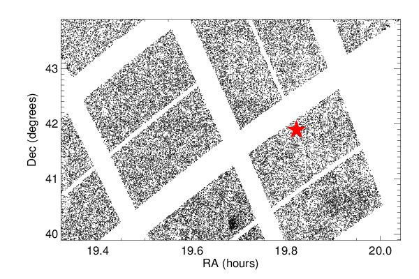
Figure 1.— A section of the Kepler footprint. Each point is a Kepler target. The red five-pointed star marks the location of KOI-94.

Nonetheless, the Kepler pipeline, as described in Batalha et al. (2012), has found 4 transiting planet candidates associated with KOI-94 (see Figure 2). The light curve is phase-folded around their transit centers in Figure 3. In summary, they are a super-Earth (KOI-94b) in a 3.7-day orbit, a mini-Neptune or super-Earth (KOI-94c) in a 10-day orbit, a Jupiter-size planet (KOI-94d) in a 22-day orbit, and a Neptune-size planet (KOI-94e) in a 54-day orbit. The Kepler Input Catalog (KIC) ascribes an effective temperature of 6217 K and a radius of 1.238 $R_{\sun}$to KOI-94, resulting in planetary radii of 1.41 $R_{\earth}$, 3.44 $R_{\earth}$, 9.26 $R_{\earth}$, and 5.48 $R_{\earth}$for planets b, c, d, and e, respectively. Our analysis of the stellar spectrum, which finds different values for the stellar temperature and radius and therefore for the planet radii, is described in §4.

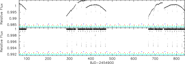
Figure 2.— The top panel shows the aperture photometry long cadence (30 minute) light-curve. No corrections have been applied to the photometric measurements. The bottom panel shows the detrended light-curve. The data were detrended by applying a 2-day median filter. Observations that occurred during a planetary transit were excluded from the calculation of the median. The triangles indicate when transits occurred for planets b, c, d, and e with corresponding colours of cyan, green, red and blue.

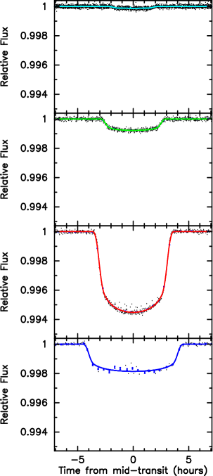
Figure 3.— The top panel shows the photometric observations phased to the orbital period of planet b with the best fit transit model overlaid. The transit models for planets c, d and e have been removed. The transit times have been corrected for transit-timing variations. The next three panels show the transit lightcurves centred on planets c, d, and e respectively. As in the upper panel, the best fit models for other transiting planet have been removed and corrected for transit timing variations. The colors of the overlaid models match the identification used in Figure 2.

3.2. Adaptive Optics

KOI-94 was observed with near-infrared adaptive optics on 2009 Nov 08 using ARIES on the MMT (Adams et al. 2012). Images were obtained in both J and Ks, and reveal no companions closer than 7.5″ ($\Delta_{J}=2.5$, $\Delta_{Ks}=2$; see Figure 4). The image FWHM was 0.23 in Ks and 0.43 in J. We can place a limit on undetected companions of $\Delta_{J}=2.2$ and $\Delta_{Ks}=3.4$ at 0.5″, $\Delta_{J}=4.6$ and $\Delta_{Ks}=5.9$ at 1.0″, and $\Delta_{J}=8.7$ and $\Delta_{Ks}=9.1$ at 4.0″(and beyond). Any additional companions that would dilute the transit light curve and change the planet parameters are constrained to be faint or very close to the star.

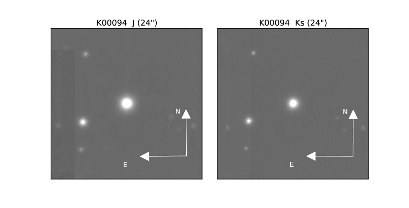
Figure 4.— Adaptive optics image of KOI-94 (center) in J and Ks. The closest companion is 7.5″ away. All of the objects in the frame are stars except for the spot in the bottom left, which is an artifact.

3.3. Speckle Imaging

Speckle imaging of KOI-94 was obtained on the night of 19 June 2010 UT and the night of 23 Oct 2010 using the two-color DSSI speckle camera at the WIYN 3.5-m telescope on Kitt Peak. The speckle camera simultaneously obtained 5000 (3000) 40 msec images on 19 June (23 Oct) in filters: $V$ (center = 5620Å, width = 400Å) , $R$ (center = 6920Å, width = 400Å) and $I$ (center = 8880Å, width = 400Å). These data were reduced and processed to produce a final reconstructed speckle image for each filter. Figure 5 shows the reconstructed R band image. North is up and East is to the left in the image and the “cross” pattern seen in the image is an artifact of the reconstruction process. The details of the two-color speckle camera observations and the Kepler follow-up observing program are presented in Howell et al. (2011).

On both occasions, the speckle data for this $R$=12.5 star allow detection of a companion star within the approximately $2.76\times 2.76$″ box centered on the target. The speckle observation can detect, or rule out, companions between 0.05″ and 1.5″ from KOI-94. The June 2010 speckle image was obtained with the WIYN telescope during relatively poor native seeing near 1.0″, while the Oct 2010 observations made during good seeing, 0.6″. We found no companion star within the speckle image separation detection limits to a delta magnitude limit of $\sim$4 mag in the R band, 2 mag in the V band, and 3.4 mag in the I band.

Figure 5.— Speckle image obtained 2012-10-23 at the WIYN telescope at 692 nm. The image spans 2.76″$\times$ 2.76″.

3.4. Spectroscopy

We obtained time-series spectroscopy of KOI-94 on the W. M. Keck I telescope with the HIRES echelle spectrometer through an iodine cell. Most of the observations occurred between May and August 2012, but our earliest observation was 2009-12-07. We rejected spectra with fewer than 4000 ADU (8760 photons), since these low-signal spectra resulted in large ($>6$ m/s) radial velocity errors. We also excluded spectra taken during a transit of KOI-94d to avoid confusion from the Rossiter-McLaughlin effect. This yielded 26 spectra that we deemed suitable for RV analysis, as presented in Table 1. We also obtained a spectrum of KOI-94 without the iodine cell as a template for RV analysis and for characterizing the star (see §4).

Note that one observation, on JD 16135.095, occurred during a transit of planet e. To see whether this datum affected our mass results, we tried removing it and repeating the circular analysis described in §4.2. Removing the datum changed the masses of the planets by $\sim.01\sigma$, and so we can safely ignore the effects of this datum on our analysis of the planetary system.

Table 1Spectroscopic Observations

JD - 2440000.0	Photons	RV	Error
		(m/s)	(m/s; Jitter = 3.0)
15172.768	9351	-9.6	6.1
16076.070	11709	27.0	5.5
16100.047	23095	14.2	5.0
16109.929	23065	-13.5	5.0
16111.048	22920	-16.8	5.0
16113.043	22594	-14.9	5.0
16114.077	14484	-17.0	6.0
16115.074	21584	-5.0	5.0
16116.054	23041	8.1	4.8
16134.015	22973	-9.2	4.9
16135.095	23592	-9.7	4.7
16139.015	22594	6.8	4.5
16140.813	22370	3.8	5.0
16144.100	20178	20.3	5.2
16144.796	23330	14.6	4.6
16146.057	18774	18.5	4.9
16147.972	22642	2.5	4.7
16149.091	15395	-13.8	5.0
16149.752	22918	6.1	4.5
16149.766	22629	-6.7	4.6
16150.065	19204	-2.6	4.8
16150.079	19162	-5.6	4.8
16150.094	18323	-10.1	4.9
16151.075	22791	-10.0	5.2
16164.001	23183	23.0	4.9
16173.925	21904	-10.7	5.1

Note. — Observations with low signal-to-noise (fewer than 8760 photons) were not used in our analysis and are omitted from this table. Photon counts are averaged over all pixels.

We determined the radial velocity of KOI-94 in each iodine spectrum based on the spectrum’s Doppler shift. We used the lab-frame iodine lines that the iodine cell superimposes on the stellar spectrum to calibrate velocities to an instrumental precision of 3 $\rm m\,s^{-1}$(although stellar jitter introduces additional errors). This technique is described in further detail in Howard et al. (2011).

4. Planet and Stellar Properties from Radial Velocities, Photometry and Spectra

We use radial velocity measurements of KOI-94 to determine the mass of planet d, marginal mass detections of planets e and b, and an upper limit on the mass of planet c. A plot of radial velocity versus time and a four-planet circular fit is shown in Figure 6.

Figure 6.— Radial velocity versus time from May 2012 onward. Black points are data with 1$\sigma$ errors (assuming a stellar jitter of 3.0 m/s); a circular four-planet fit is superimposed.

We fit the RVs with three models, each of which provides an interesting interpretation of the system. The first model has only one planet (the giant) in a circular orbit. This is because the giant planet dominates the RVs, and so it is useful to compare a four-planet solution to a simpler one-planet solution. In our second model, all four planets are in circular orbits. Because KOI-94 is a closely-packed system, we do not expect large eccentricities of the planets, so we want to verify that a solution allowing eccentricities is not significantly different from a circular solution. In our third and most sophisticated model, we fit for all four planets in eccentric orbits while simultaneously fitting the light curve.

4.1. Circular Orbit Solutions

Here we compare the results of the one-planet and four-planet circular orbital solutions. For the one-planet fit, we find $K=16.3\,\rm m\,s^{-1}$, producing a reduced $\chi^{2}$ of 1.97. The data and phase-folded, one-planet circular fit are shown in Figure 7.

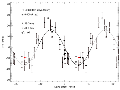
Figure 7.— A one-planet, circular fit to the RVs, phase-folded to the period of KOI-94d. The black points are the data (error bars are $1\sigma$), and the black line is the circular one-planet fit to the data. The gray points and fit are time-shifted repetitions of the black data points and fit. The red point is the oldest data point (2009); all other data are from summer 2012.

In the four-planet circular model, the center-of-mass velocity $\gamma$ of the system and the semi-amplitude $K_{n}$ of each planet $n$ are allowed to vary, allowing 5 degrees of freedom; all other orbital parameters are fixed. We augmented the photon-noise errors by 3.0 $\rm m\,s^{-1}$in quadrature to account for the stellar jitter. The best four-planet fit had a reduced $\chi^{2}$ of 1.60. The best-fit radial velocity components from the four planets are shown in Figure 8.

Because the stellar jitter is unknown, we recalculated this fit, varying the stellar jitter to achieve $\chi^{2}=1$ (this yielded a jitter of 5.0 $\rm m\,s^{-1}$). The RV semi-amplitudes achieved in this fit were consistent with those assumed for a stellar jitter of 3.0 $\rm m\,s^{-1}$: the semi-amplitude for KOI-94d and KOI-94e changed by less than half a percent, and the semi-amplitudes for KOI-94b and KOI-94c fell within the $1\sigma$ errors. We also note that because these are circular fits, the difference in $\chi^{2}$ between a model with a stellar jitter of 3.0$\rm m\,s^{-1}$ and 5.0$\rm m\,s^{-1}$ could arise from planetary eccentricities that are excluded from the model. Therefore, we assume a stellar jitter of 3.0 $\rm m\,s^{-1}$ and adopt the resulting parameters for the 4-planet circular solution, which are reported in Table 2.

Table 2Planet parameters for circular orbits of KOI-94.

Parameter	Value
Circular Keplerian Fit: KOI-94b
Center-of-mass velocity $\gamma$ ($\rm m\,s^{-1}$)	$1.76\pm 1.4$
Orbital semi-amplitude $K$ ($\rm m\,s^{-1}$)	$3.2\pm 1.7$
Mass $M_{\rm P}$ ($M_{\earth}$)	$9.2\pm 4.9$
Density $\rho_{\rm P}$ ($\rm g\,cm^{-3}$)	$9.0\pm 4.7$
Circular Keplerian Fit: KOI-94c
Orbital semi-amplitude $K$ ($\rm m\,s^{-1}$)	$1.6\pm 1.3$
Mass $M_{\rm P}$ ($M_{\earth}$)	$6.5\pm 6.3$
Density $\rho_{\rm P}$ ($\rm g\,cm^{-3}$)	$0.46\pm 0.37$
Circular Keplerian Fit: KOI-94d
Orbital semi-amplitude $K$ ($\rm m\,s^{-1}$)	$19.68\pm 2.19$
Mass $M_{\rm P}$ ($M_{\earth}$)	$102\pm 11.4$
Density $\rho_{\rm P}$ ($\rm g\,cm^{-3}$)	$0.380\pm 0.042$
Circular Keplerian Fit: KOI-94e
Orbital semi-amplitude $K$ ($\rm m\,s^{-1}$)	$5.25\pm 2.04$
Mass $M_{\rm P}$ ($M_{\earth}$)	$36.6\pm 14.4$
Density $\rho_{\rm P}$ ($\rm g\,cm^{-3}$)	$0.690\pm 0.268$

Note. — The best fit parameters for four planets in circular Keplerian orbits, after adopting stellar parameters and orbital ephemerides from the eccentric solution described in §4.2 (see Table 3).

We assessed the errors in $K_{n}$ with a Markov Chain Monte Carlo (MCMC) analysis of 1 chain of 10⁷ trials using the Metropolis-Hastings algorithm. Figure 9 shows the posterior likelihood distributions. The corresponding planet mass ($M_{\rm P}$) and density ($\rho_{\rm P}$) distributions (which are calculated from the orbital period and planet radius) are also shown. These parameters are reported in Table 2.

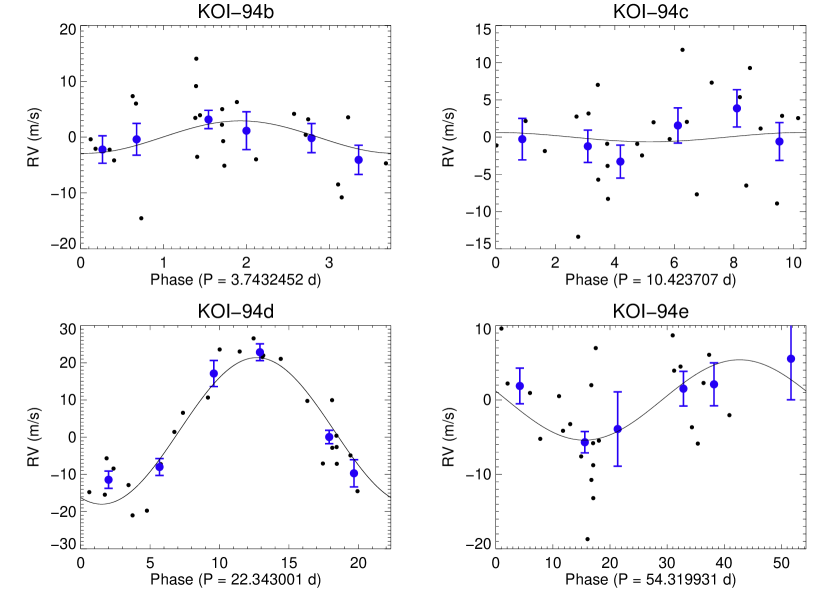
Figure 8.— Radial velocity components from a four-planet circular fit. Each panel shows the radial velocity signature from one planet. The black line is the model fit; the black points are the RV data minus the model RVs from the other three planets. The blue points are the binned RVs. We chose the number of bins by rounding up the square root of the number of observations, creating 6 bins of equal spacing in phase. The error bars are the uncertainty in the mean of the data in each bin. The reduced $\chi^{2}$ of this fit is 1.60. The RVs provide a $9\sigma$ detection of KOI-94d, a $2.5\sigma$ detection of KOI-94e, a $2\sigma$ detection of KOI-94b and an upper limit on the mass of KOI-94c.

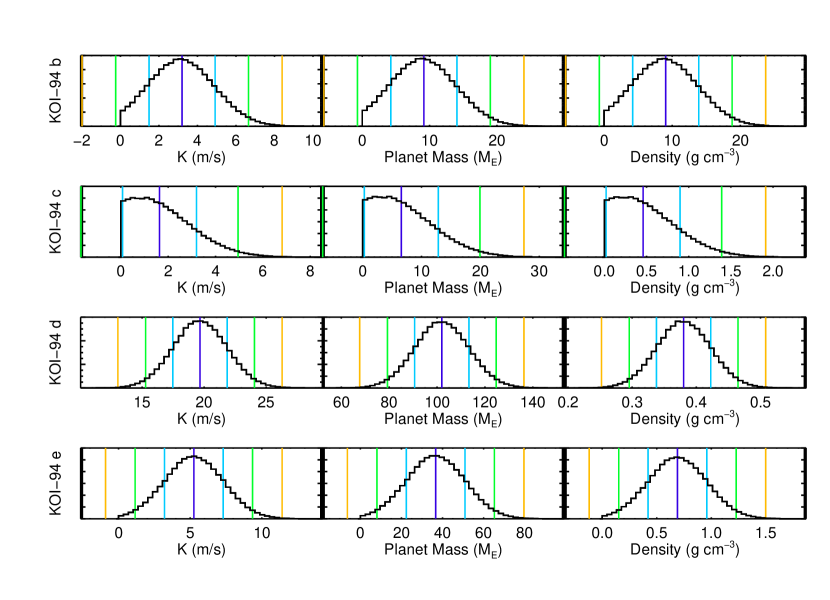
Figure 9.— Posterior distributions for the four-planet circular fit. From left to right: likelihoods of $K$, $M_{P}$, and $\rho_{P}$ for (top to bottom) KOI-94b, KOI-94c, KOI-94d, and KOI-94e. The median, $1\sigma$, $2\sigma$, and $3\sigma$ likelihoods are over-plotted in dark blue, cyan, green, and orange. To account for the positive definite bias of the likelihood distribution, $\sigma$ is measured above the median only; lower bounds are reflections of the upper bounds (i.e., a symmetric distribution is assumed). This enables a quantitative estimate of the number of trials consistent with a non-detection via RVs. Note that the best-fit values are obtained by minimizing $\chi^{2}$; the posterior distributions are used only for estimating uncertainties. The best-fit values and uncertainties for the circular orbits are presented in Table 2.

To calculate the probability of a non-detection in RVs for each planet, we assume a Gaussian posterior distribution and calculate the fraction of trials that would have occurred for masses at or below zero, had we not imposed a positive definite value for $K_{n}$. We calculate the following probabilities of a non-detection via RVs: 0.04 for planet b, 0.14 for planet c, $5\times 10^{-19}$ for planet d, and 0.007 for planet e. However, these estimates of the non-detection probability are smaller than the true probability of non-detection because of the Lutz-Kelker bias, especially for planet c.

4.1.1 Limiting Outer Planets

The absence of a significant change in the radial velocity of the star between our earliest and most recent measurements strongly limits the possibility of a massive outer companion. To quantify this, we computed a circular, four-planet orbit solution in which we allowed a linear trend in the radial velocity as a free parameter and used an MCMC analysis to explore the likelihood of a given linear velocity trend. Over a two-year baseline, the median trend was $-0.0125\pm 0.0063$  $\rm m\,s^{-1}$ per day, which corresponds to a $3\sigma$ upper limit of -6.9 $\rm m\,s^{-1}$ per year. In the style of Winn et al. (2010), we compute the mass of an outer perturber based on the stellar acceleration, $\dot{\gamma}$, assuming the planet induces Newtonian gravitational acceleration on the star and in the limit $M_{\rm P}\ll M_{\star}$: $\dot{\gamma}=GM_{\rm P}/a^{2}$. To induce a stellar acceleration $\dot{\gamma}$ of -6.9 $\rm m\,s^{-1}$ per year via Newtonian gravity, an outer perturber would need to satisfy

$$\frac{M_{\rm P}\mathrm{sin}i}{M_{\rm J}}\left(\frac{a}{10\ \mathrm{AU}}\right)^{-2}=3.9,$$ (3)

where $i$ is the inclination of the planet’s orbital plane with respect to the line of sight and $M_{\rm J}$ is the mass of Jupiter. Thus, with a significance of $3\sigma$, we can rule out companions more massive than 3.9 $M_{\rm J}$ within 10 AU or more massive than 1.0 $M_{\rm J}$ within 5 AU.

4.2. Eccentric Orbit Solution

The four-planet fit in which we allow eccentricities to float is the most versatile model. This model has the advantage of simultaneously fitting the light curve and the RVs, which measures $\rho_{\star}$ (thus refining $M_{\star}$ and $R_{\star}$). As demonstrated below, the values for planet masses in this model agree with the planet masses determined in the circular orbital solution to within $1\sigma$, and so we adopt the parameters from the eccentric solution for the rest of this work.

The Kepler photometry and Keck radial velocities were simultaneously fit with an orbital model. The model has the following free parameters: mean stellar density ($\rho_{\star}$), scaled planetary radius ($r_{n}/R*$), impact parameter ($b_{n}$), orbital period ($P_{n}$), center of transit time ($T_{c,n}$), radial velocity amplitude ($K_{n}$), eccentricity ($e_{n}$) and argument of pericenter ($w_{n}$) via esin$w_{n}$ and ecos$w_{n}$. A photometric and radial velocity zero point were also included. The number (n=1,2,3,4) corresponds to the parameters for planet b,c,d and e respectively. The transit model uses the quadratic formulae of Mandel & Agol (2002). Limb-darkening coefficients were fixed in the models to 0.3236 and 0.3052 as determined from the grid of Claret & Bloemen (2011). The orbits are modeled with non-interacting Keplerians.

A best-fit model was initially computed by minimizing $\chi^{2}$ with a Levenberg-Marquardt style algorithm. This model was used to measure TTVs and to seed an MCMC analysis of the model parameter space. TTVs were determined by fitting for each individual transit, fixing all parameters except $T_{c}$ to their best-fit values. An updated best-fit model was then computed using the TTVs to produce a better phased transit for each planet. The time-series were corrected by computing time-corrections based on a linear-interpolation of the TTVs.

Posterior distributions for each model parameter were determined with an MCMC-style algorithm. This model has been described in Gautier et al. (2012a) and Borucki et al. (2012), the only difference is that the TTV measurements are included and fixed to their best-fit values. Four Markov-chains were calculated each with a length of $10^{6}$. The first 10% of each chain was discarded as burn-in. The median and $\pm 1\sigma$ percentiles were calculated for each model parameter and reported in Table 3, which is in the appendix due to its length.

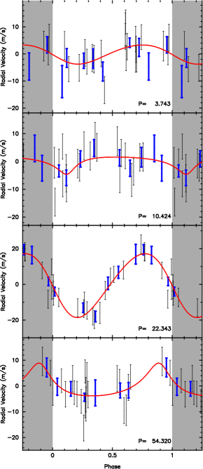
Figure 10.— Radial velocity components from the four-planet eccentric fit in which the photometry and radial velocities were fit simultaneously. Each panel shows the radial velocity signature from one planet (top to bottom: b, c, d, e). The red line is the model fit; the black points are the RV data minus the model RVs from the other three planets. The blue points are the binned RVs; their error bars the uncertainty in the mean. The shaded regions show phase-shifted repetitions of the data and fit.

4.2.1 Stellar Properties

We used the template spectrum (without iodine) to determine the effective temperature ($T_{\rm eff}$= $6182\pm 58$), surface gravity ($\log{g}$= $4.181\pm 0.066$), and metallicity ([Fe/H]= $+0.0228\pm 0.0020$) of KOI-94 through the Spectra Made Easy (SME) analysis technique described in Valenti & Piskunov (1996). Applying the evolutionary constraints of the Yi et al. (2001) model isochrones and the simultaneous solution of the lightcurve and RVs, we determine the mass ($M_{\star}=1.277\pm 0.050$) and radius ($R_{\star}=1.52\pm 0.14$) of KOI-94. The stellar properties are presented in Table 3.

4.2.2 Properties of KOI-94d from the Eccentric Orbit Solution

We detect KOI-94d with 9$\sigma$ confidence with the RVs. The eccentric orbit analysis gives a mass of $106\pm 11$$M_{\earth}$. This mass is marginally consistent with the mass reported by Hirano et al. (2012), who found $M_{\rm P}=73\pm 25$ $M_{\earth}$.

4.3. Planet Masses from Transit Timing Variations.

We observe coherent TTVs for KOI-94c and KOI-94d  which are presented in Figure 11. TTVs usually indicate gravitational interactions between adjacent pairs of planets; such interactions allow us to refine the mass estimates of these planets.

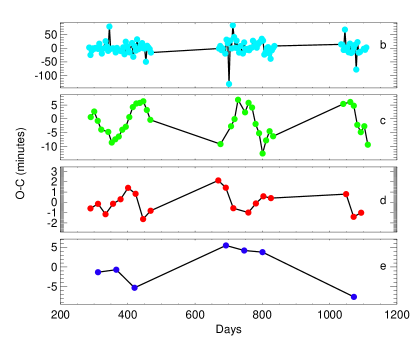
Figure 11.— Observed Transit Timing Variations in Q1-Q12 for (top to bottom) KOI-94b, KOI-94c, KOI-94d, and KOI-94e, with the same color scheme as Figures 2 and 3. The y-axis of each plot shows the difference between the observed transit time (O) and the transit time expected for a periodic orbit (C). Days are in JD$-$2454900. The errors are smaller than the point size. We excluded one $5.5\sigma$ outlier in the O-C measurements for planet c at 686 days. There is a section between days 650 and 800 in which the TTVs of planets c and d are anti-correlated, indicating a possible gravitational interaction.

We use the prescription of Equations 8 and 9 from Lithwick et al. (2012) to predict the anti-correlated TTV signals produced during the interaction of planets c and d between 650 and 800 days. Assuming zero eccentricity for both planets and ignoring factors of order unity, we calculate

$$V=P\frac{\mu^{\prime}}{\pi j^{(2/3)}(j-1)^{(1/3)}\Delta}$$ (4)

$$V^{\prime}=P^{\prime}\frac{\mu}{\pi j(j-1)^{(1/3)}\Delta}$$ (5)

where $\mu$ is the ratio of the inner planet mass to the stellar mass, $\mu^{\prime}$ is the ratio of the outer planet mass to the stellar mass, $V$ is the predicted semi-amplitude of the complex TTV signal for the inner planet, and $V^{\prime}$ is the predicted semi-amplitude of the complex TTV signal for the outer planet. $\Delta$, which is given by

$$\Delta=\frac{P^{\prime}}{P}\frac{j-1}{j}-1$$ (6)

is the fractional departure from a $j:j-1$ mean motion resonance.

Using the values for the orbital periods of planets c and d, for which the closest first-order mean motion resonance is 2:1, we calculate $\Delta=0.074.$ Using the SME-determined mass of the star and the RV-determined planet masses, we calculate $V=7$ minutes and $V^{\prime}=1.7$ minutes. These values agree with the observed TTV interaction in Figure 11, for which the TTV amplitudes of planets c and d appear to be about 7 and 1 minutes, respectively.

4.4. Dynamical Stability

We investigate the long-term stability of the KOI-94 system. We integrate the orbits of all four planets using the built-in hybrid symplectic/Bulirsch-Stoer integrator, part of the Mercury software package (Chambers 1999). We use the orbital and physical parameters of the four planets detailed in Table 3. The mean anomalies are derived from the best-fit joint radial-velocity solution. We define in the following a non-stable system when a close encounter between a given body and one of the four others occurs, within their common Hill radius. In a first set of 1-Myr integrations, fifteen eccentricity values for each planet are randomly drawn from the normal distribution $N(e,\sigma_{e}^{2})$, where $e$ is the best-fit orbital eccentricity and $\sigma_{e}$ is the $1\sigma$ eccentricity uncertainty. Eighty percent of these integrations yield close encounters between the two innermost planets b and c. Closer inspection of the results reveal that the proximity of b and c put stringent constraints on their orbital eccentricity, only allowing values less than or equal to the best-fit values for the system to be stable.

In a second set of ten integrations, all planets are restricted to circular orbits with masses drawn from their normal distributions, in a similar manner as for orbital eccentricity in the previous step. All integrations with circular orbits resulted in stable systems, showing that varying planetary masses within their $1\sigma$ uncertainty has a negligible influence on the dynamical stability of the system, if orbits are kept circular.

More detailed dynamical analyses of the KOI-94 system would determine an upper limit on orbital eccentricity for the b and c components. This would however imply arbitrary assumptions on planetary masses, which would not completely exclude configurations with large orbital eccentricities. A possible resolution would be to precisely determine the planetary masses of the close-in components, either through additional RV observations or an N-body analysis of the TTV signals from these planets.

5. Support for the Existence of the Planets

In this work, we sought to measure the mass of the warm Jupiter KOI-94d to determine how the planet compared to the population of hot Jupiters. We simultaneously fit the Kepler light curve and 26 RVs from Keck/HIRES to measure the mass of KOI-94d with a statistical significance of $9\sigma$. We also sought to measure the masses of the other three transiting planet candidates in KOI-94 in order to better understand the architecture of this planetary system. Our RV measurements of KOI-94 measure the masses of the other planets with signficances of less than 3$\sigma$ (see Tables 2 and 3). However, other observations we have made support the interpretation of KOI-94 as a system with four transiting planets. We describe support for the planetary interpretation of the candidates below. We defer our discussion of the comparison of KOI-94d to other Jupiter-size planets to the next section.

We report the properties of planets KOI-94b ($M_{\rm P}$= $10.5\pm 4.6$$M_{\earth}$, $R_{\rm P}$= $1.71\pm 0.16$$R_{\earth}$), KOI-94c ($M_{\rm P}$= $15.6^{+5.7}_{-15.6}$$M_{\earth}$, $R_{\rm P}$= $4.32\pm 0.41$$R_{\earth}$), KOI-94d ($M_{\rm P}$= $106\pm 11$$M_{\earth}$, $R_{\rm P}$= $11.27\pm 1.06$$R_{\earth}$), and KOI-94e ($M_{\rm P}$= $35^{+18}_{-28}$$M_{\earth}$, $R_{\rm P}$= $6.56\pm 0.62$$R_{\earth}$). Although the fidelity of the Kepler candidates is very high ($90-95\%$ according to Morton & Johnson 2011, see Fressin et al. (in prep) for an estimate of fidelity as a function of planetary radius), false positives do exist among the Kepler planet candidates in the form of background eclipsing binaries, hierarchical triples, and other configurations of stars that result in the dilution of the eclipse signal, allowing it to masquerade as a planetary transit. The large size of Kepler pixels renders Kepler particularly vulnerable to bound companion stars with a large planet, such as a Neptune- or Jupiter-size planet, mimicking the transit signal of an Earth-size planet. To show that a planetary interpretation is superior to the interpretation of these various false positive signals, we outline the various measurements and statistical properties of the KOI-94 system that support the hypothesis of four transiting planets.

5.1. Radial Velocities from KOI-94d

The eccentric orbit solution of the RVs and light curve yield a semi-amplitude of $18.3\pm 1.5$ $\rm m\,s^{-1}$ with a 22.3 day period for KOI-94d. Similarly, the four-planet circular orbit solution yields a semi-amplitude of $19.68\pm 2.19$ $\rm m\,s^{-1}$ to the RVs. The agreement between the circular and eccentric values for the semi-amplitude of KOI-94d underscores the robustness of this measurement.

At a 22-day period, a semi-amplitude of $18.3\pm 1.5$ $\rm m\,s^{-1}$ is consistent with the orbit of a planet around a star. A binary star system in 22-day period would have a velocity semi-amplitude of hundreds of kilometers per second. The width of the spectral lines is consistent with a stellar rotation speed of 8 $\mathrm{kms^{-1}}$, which is at least an order of magnitude smaller than the orbital speed of a such a binary system. Thus, we rule out the possibility of an eclipsing binary false positive in a 22-day orbital period for KOI-94d. This supports the interpretation of KOI-94d as a planet. As discussed below, the planetary status of KOI-94d strengthens the case that the other transiting candidates are also planets.

5.2. Observed TTV signature between KOI-94c and KOI-94d

The apparent anti-correlation in the TTVs between planets c and d from 700-800 days (see Figure 11 suggests that these bodies are dynamically interacting, i.e. that KOI-94c is also a planet. Our order-of-magnitude treatment of the TTV signatures indicates that the interacting bodies are of planetary masses, although the mass estimates are too low by a factor of 5.

5.3. No Evidence of Another Star

The adaptive optics images show no evidence of companions as close as 0.5″ from KOI-94 within 2 magnitudes in the J band or 3.4 magnitudes in the Ks band. Similarly, the speckle imaging shows no evidence of companions as close to KOI-94 as 0.6″ within 4 magnitudes in the R band. Also, the $3\sigma$ upper limit on an RV trend of $\dot{\gamma}=6.9$ $\rm m\,s^{-1}$ per year between fall 2009 and fall 2012 rules out a Jupiter-mass or more massive companion within 5 AU.

The detection of a second stellar spectrum in the spectrum of KOI-94 would indicate background or companion star. We searched for the spectrum of a second star in the iodine-free HIRES spectrum of KOI-94. To fit the spectrum of the primary star (KOI-94), we used a library of over 700 observed spectra from Keck HIRES that span $T_{\rm eff}$: $3266\,\mathrm{K}-7258\,\mathrm{K}$, $\log{g}:1.46-5.0$, and [Fe/H]:$-1.47-+0.56$. We found the spectrum from this library with the least squares difference from the spectrum of KOI-94 (with similar results to the SME analysis) and subtracted this spectrum. We then compared the residual spectrum to each spectrum in the stellar library. The deepest minimum in $\chi^{2}$ between the residual spectrum and another star from the library was $2\sigma$ at $-59.2\rm km\,s^{-1}$; however, there were many other 2$\sigma$ solutions for that spectrum. We did not detect a second stellar spectrum with $>1\%$ of the observed brightness of KOI-94 and a relative radial velocity of at least $\sim 8\,\rm km\,s^{-1}$ with $>2\sigma$ significance. This technique is sensitive only to neighboring stars within 0.4″, the half-width of the slit of the HIRES spectrometer.

5.4. Low False Positive Rate in Multi-Planet Systems

Lissauer et al. (2012) uses statistical arguments to calculate the false positive fraction in multi-planet systems. Given the observed number of Kepler targets $n_{t}$, the number of Kepler planet candidates $n_{c}$, the number of Kepler multi-planet systems with $i$ planet candidates $n_{m,i}$, and the planet fidelity $P$ (or single candidate false positive rate $1-P$), the fraction of systems with four planet candidates that we expect to consist of one false positive and three true planets ($\mathrm{P_{1FP}}$) is equivalent to the probability that a false positive is lined up behind a system that already has three true planets. The number of false positives among the candidate transiting planets is $(1-P)n_{c}$, and the fraction of those aligned with apparent $i$-planet systems is $n_{m,i}/n_{t}$. Thus,

$$\mathrm{P_{1FP}}=\frac{(1-P)n_{c}\frac{n_{m,4}}{n_{t}}}{n_{m,4}}=\frac{(1-P)n_{c}}{n_{t}}.$$ (7)

Adopting the values $n_{t}=160171$ from Lissauer et al. (2012) and $n_{c}=2300$ from Batalha et al. (2012), and assuming $P=0.9$ (in accordance with Morton & Johnson 2011), we calculate

$$\mathrm{P_{1FP}}=0.0014.$$

The probability that 2, 3, etc. planet candidates are all false positives (un-associated eclipsing binaries that all happen to align behind KOI-94 within 0.5″) is orders of magnitude smaller and can be ignored. The low false positive probability is definitive of planethood even without the other arguments presented in this section.

5.5. Rossiter-McLaughlin Measurement During the Transit of KOI-94d

Hirano et al. (2012) measured the Rossiter-McLaughlin (RM) effect during transit of KOI-94d. They observed a clear RM signal that, when measured considering a transit depth of $R_{\rm P}/R_{\star}=0.06856\pm 0.00012$, implied a projected stellar rotation of $V\mathrm{sin}I_{s}=8.01\pm 0.73\rm km\,s^{-1}$, which is in good agreement with their spectroscopically determined value of $7.33\pm 0.32\rm km\,s^{-1}$ and our SME analysis. This constitutes evidence for the planetary status of KOI-94d. Albrecht et al. (2013) also measured and modeled the RM effect during the same transit of KOI-94dand obtained results that agreed with Hirano et al. (2012).

Modeling of the transit durations, including ingress and egress, of the KOI-94 transit candidates indicate small inclinations with respect to the line of sight (see the inclinations in Table 3. Hirano et al. (2012) measure a projected mutual inclination between planets d and e of $\delta=-1.5^{\circ}$ during a mutual transit event, indicating that these bodies are coplanar. That these planets are aligned with the stellar spin axis strengthens the argument for their planetary status. Recent work by Fabrycky & Kepler Science Team (2012) shows that many Kepler multi-planetary systems are coplanar, so it is likely that planets b and c are coplanar with planets d and e.

6. Constraints on the Composition of KOI-94d

The goal of this work was to measure the mass of the giant planet, KOI-94d, and determine whether its bulk density was consistent with that of an inflated or a cold Jupiter.

We have modeled the thermal evolution and contraction of planet d using the methods described in Fortney et al. (2007) and Miller & Fortney (2011). This model assumes no extra heat source from the star. Including uncertainties in the system age, planet mass, planet radius, orbital semi-major axis, and heavy element distribution within the planet (see Miller & Fortney 2011) we estimate that $18\pm 6$ $M_{\earth}$ of heavy elements are contained within the planet. This is very similar to estimates for Saturn (Saumon & Guillot 2004). Based on the [Fe/H] of the parent star determined from our SME analysis of the spectrum, we estimate that the metals mass-fraction of planet d ($Z_{\rm planet}$) is $11\pm 4$ times that of the parent star. This metallicity enhancement, at this planet mass, agrees well with other “warm Jupiter” planets studied by Miller & Fortney (2011).

We use state of the art thermal evolution models for giant planets to establish that the bulk density of the planet is fully consistent with a non-inflated planet, and it is indeed enhanced in heavy elements compared to its parent star, in a manner similar to Saturn. We can furthermore compare KOI-94d to other planets by creating mass-radius and mass-density plots for all planets with measured radius and mass (see Figure 12). These plots demonstrate the dependence of planetary radius (and density) on mass and incident flux.

7. The Radius-Mass-Incident Flux Relation

In this section, we examine empirical relations between the radius, mass and incident flux of exoplanets, including the KOI-94 system. We discuss possible physical interpretations of these relations and suggest avenues of future theoretical investigation.

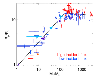
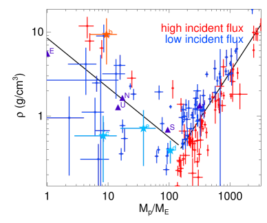
Figure 12.— All planets with measured mass, radius, incident flux, and uncertainties therein, as listed in exoplanets.org (Wright et al. 2011, see Table 4). KOI-94 planets are plotted as five-pointed stars; Solar system planets are plotted as triangles. Left: Planet radius vs. planet mass. We divide the planets into two populations: those with higher-than-median incident flux (red), and those with lower-than-median incident flux (blue) The Solar system planets (purple) all receive less than the median incident flux; KOI-94 planets c, d, and e (cyan) receive less than the median incident flux, while KOI-94b (orange) receives more than the median incident flux. For $M_{\rm P}>150M_{\earth}$, higher incident flux correlates with larger planetary radius. For $M_{\rm P}<150M_{\earth}$, higher incident flux ($F$) correlates with smaller planetary radius. The best-fit planes $\text{for }M_{\rm P}<150M_{\earth}$ and $\text{for }M_{\rm P}>150M_{\earth}$ are shown at the median flux $F=8.6\times 10^{8}\ \rm erg\,s^{-1}\,cm^{-2}$. Right: Planet density vs. planet mass. The coloring is the same as in the left panel, and the density fits $\text{for }M_{\rm P}<150M_{\earth}$and $\text{for }M_{\rm P}>150M_{\earth}$are shown at the median flux. For $M_{\rm P}>150M_{\earth}$, higher incident flux correlates with lower bulk density. For $M_{\rm P}<150M_{\earth}$, higher incident flux correlates with higher bulk density. We determine empirical relations (see text) between log($M_{\rm P}$), log($F$), and each log($R_{\rm P}$) and log($\rho_{\rm P}$) for $M_{\rm P}>150M_{\earth}$ and $M_{\rm P}<150M_{\earth}$.

This population of planets was compiled from exoplanets.org (Wright et al. 2011), which was queried on September 27, 2012. Our selection criteria were that the mass and radius of the planet were measured, and that errors in these measurements were reported, that the effective temperature and radius of the star were measured with errors reported, and that the semi-major axis was measured with errors reported. This resulted in the sample of 138 exoplanets listed in Table 4.

The methods for determining the radius, mass, and incident flux of the planets in Table 4 were as follows: All the planets transit, and so their radius measurement was based on transit depth as determined within a self-consistent model of the observed light curve. For many of these planets, the uncertainty in planet radius is dominated by the uncertainty in stellar radius. The masses of the planets were measured by one of two methods: the majority were measured as $M_{\rm P}$sin$i$ based on the radial velocity of the star; however, in several Kepler systems of multiple planets, TTVs aided (Cochran et al. 2011, Kepler-18) or provided the sole means (Lissauer et al. 2011, Kepler-11) of planetary mass calculation. Uncertainties in the planet mass stem from uncertainties in the stellar mass, uncertainties in the RV semi-amplitude $K$ for low-mass planets, and uncertainties in the TTV analysis. The incident flux for each planet was calculated using Equation 1, so uncertainties in the incident flux relate to uncertainties in stellar effective temperature, stellar radius, and semi-major axis.

There is a break in the mass-radius relation at $\sim$150 $M_{\earth}$ (see Figure 12). We chose 150 $M_{\earth}$ as the break based on a visual inspection of the mass-radius and mass-density diagrams. In determining the relation between planet radius, planet mass, and incident flux, we consider planets more or less massive than 150 $M_{\earth}$ separately. Our sample included 35 planets with $M_{\rm P}$$<$ 150 $M_{\earth}$ and 103 planets with $M_{\rm P}$$>$ 150 $M_{\earth}$. All four planets in the KOI-94 system are included in the low-mass population.

To determine how incident flux affects radius, we calculated the time-averaged incident flux on each exoplanet from Equation 1. We divided the population into the “high incident flux” half (those with incident fluxes larger than the median incident flux, $F_{m}=8.6\times 10^{8}\rm erg\,s^{-1}\,cm^{-2}$), and the “low incident flux” half. These are shown in Figure 12 as the red (high flux) and blue (low flux) sets of points. For planets with $M_{\rm P}>150M_{\earth}$, the planets that receive high incident flux are systematically larger than planets that receive low incident flux.

We performed a similar test to determine how the orbital period affects radius (see Figure 13). We divided the exoplanet population into those with lower than the median orbital period of 3.52 days (red, “short period”) and higher than the median orbital period (blue, “long period”). Planet radius does not correlate with orbital period.

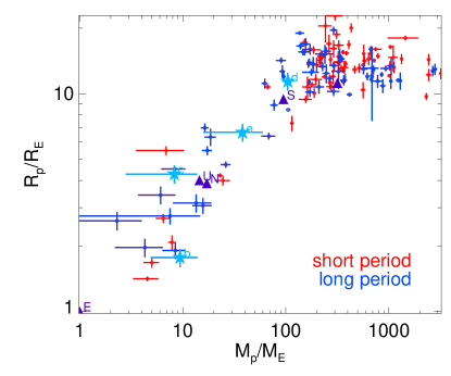
Figure 13.— Planet radius vs. planet mass (same Figure 12, but with a different coloring scheme). We divide the planets into those with lower-than-median orbital periods (red) and those with higher-than-median orbital periods (blue). The Solar System planets (purple) and KOI-94 planets b, c, d, and e (cyan) all have longer than the median period. Orbital period does not correlate with planet radius.

Using the KOI-94 system and all other exoplanets with published values for both mass and radius, we establish two fundamental planes for exoplanets that relate their mass, incident flux, and radius from a few Earth masses up to ten Jupiter masses. We fit two planes between log($R_{\rm P}$), log($M_{\rm P}$), and log($F$), one in each mass regime. The resulting relations are:

$$\begin{split}\frac{R_{\rm P}}{R_{\earth}}=1.78~{}\left(\frac{M_{\rm P}}{M_{\earth}}\right)^{0.53~{}}\left(\frac{F}{\rm erg\,s^{-1}\,cm^{-2}}\right)^{-0.03~{}}\\ \text{for }M_{\rm P}<150M_{\earth}\end{split}$$ (8)

and

$$\begin{split}\frac{R_{\rm P}}{R_{\earth}}=2.45~{}\left(\frac{M_{\rm P}}{M_{\earth}}\right)^{-0.039~{}}\left(\frac{F}{\rm erg\,s^{-1}\,cm^{-2}}\right)^{0.094~{}}\\ \text{for }M_{\rm P}>150M_{\earth}\end{split}$$ (9)

For completeness, we also fit two planes between log($\rho_{\rm P}$), log($M_{\rm P}$), and log($F$):

$$\begin{split}\frac{\rho_{\rm P}}{\rm g\,cm^{-3}}=1.30~{}\left(\frac{M_{\rm P}}{M_{\earth}}\right)^{-0.60~{}}\left(\frac{F}{\rm erg\,s^{-1}\,cm^{-2}}\right)^{0.09~{}}\\ \text{for }M_{\rm P}<150M_{\earth}\end{split}$$ (10)

and

$$\begin{split}\frac{\rho_{\rm P}}{\rm g\,cm^{-3}}=0.48~{}\left(\frac{M_{\rm P}}{M_{\earth}}\right)^{1.10~{}}\left(\frac{F}{\rm erg\,s^{-1}\,cm^{-2}}\right)^{-0.28~{}}\\ \text{for }M_{\rm P}>150M_{\earth}\end{split}$$ (11)

Table 4 lists the mass, radius, incident flux, orbital period, and reference for the planets used to calculate these fits. We include the Solar system planets in Figure 12 for reference, although these planets were not used to generate the fits in Equations 8$-$11. Slice through the planes at the median incident flux is shown as black lines in Figure 12.

These planes were calculated by fitting a plane to the measurements of log$M_{\rm P}$, log$R_{\rm P}$, and log$F$ in each mass regime, with equal weight for each point. To see how the uncertainties in $M_{\rm P}$, $R_{\rm P}$, and $F$ influenced the fit, we did 1000 trials in which we varied each measurement of $M_{\rm P}$, $R_{\rm P}$, and $F$ based on a Gaussian distribution with the $1\sigma$ uncertainties reported for that planet to create a posterior distribution of coefficients. The median and average values for the posterior distribution of the coefficients were consistent with the coefficients of the original fit. If we write Equations 8 and 9 more generally as $\mathrm{log}(R_{\rm P}/R_{\earth})=A+B\mathrm{log}(M_{\rm P}/M_{\earth})+C\mathrm{log}(F/\rm erg\,s^{-1}\,cm^{-2})$, the $1\sigma$ uncertainties in the coefficients for Equation 8 (i.e. $\text{for }M_{\rm P}<150M_{\earth}$) are $A=0.25\pm 0.185$, $B=0.53~{}\pm 0.052$, and $C=-0.03~{}\pm 0.017$. The $1\sigma$ uncertainties in the coefficients for Equation 9 (i.e. $\text{for }M_{\rm P}>150M_{\earth}$) were $A=0.39\pm 0.053$, $B=-0.039~{}\pm 0.0096$, and $C=0.094~{}\pm 0.0055$. Thus, the dependence of radius on mass for low-mass planets is significant at $10\sigma$, and the dependence of radius of flux for high-mass planets is significant at $17\sigma$. The downward slope of radius versus mass for giant planets is detected at a significance of $4\sigma$, and the downward slope of radius versus flux for small planets is uncertain.

For $M_{\rm P}<150M_{\earth}$, the RMS scatter of the radius is 1.41$R_{\earth}$ and the RMS scatter of the density is 2.69$\rm g\,cm^{-3}$. Considering that the average radius of a planet in this mass regime is 6.72$R_{\earth}$ and the average uncertainty in planet radius in this mass regime is 0.34$R_{\earth}$(i.e. 5% of the typical planet radius), the RMS scatter of radii for $M_{\rm P}<150M_{\earth}$ is large compared to the uncertainties in measurements of planet radii. For $M_{\rm P}>150M_{\earth}$, the RMS scatter of the radius is 1.15$R_{\earth}$ and the RMS scatter of the density is 1.48$\rm g\,cm^{-3}$. Considering that the average uncertainty in planet radius $\text{for }M_{\rm P}>150M_{\earth}$ is 0.76$R_{\earth}$, the RMS scatter is comparable to the uncertainty in planet radius in this mass regime. Interpretations of the RMS scatter in each mass regime is discussed in §7.1.

Note than $\text{for }M_{\rm P}<150M_{\earth}$, radius depends strongly on mass ($R_{\rm P}\propto M_{\rm P}^{0.52}$) and very weakly on incident flux ($R_{\rm P}\propto F^{-0.03}$). For $M_{\rm P}>150M_{\earth}$, the dependence is reversed: $R_{\rm P}\propto M_{\rm P}^{-0.04}$, and $R_{\rm P}\propto F^{0.09}$. Since mass has little effect on radius for giant planets, the incident flux is the most important factor in predicting planet radius.

In light of the very clear dependence of giant planet radius on incident flux, and the possibility of a dependence of low-mass planet radius on incident flux, we wanted to examine the relations between incident flux and planet radius in greater detail. The top panel of Figure 14 shows planet radius as a function of incident flux for the low-mass and high-mass planets. The scatter in radius of the low-mass planets can be attributed to the strong dependence of planetary radius on mass $\text{for }M_{\rm P}<150M_{\earth}$. However, the relation between the radii of giant planets and the incident flux is clear in this plot because the dependence of planet radius on mass is very small $\text{for }M_{\rm P}>150M_{\earth}$.

It appears that for planets with $M_{\rm P}<150M_{\earth}$, the planets receiving high incident flux are systematically smaller than planets receiving low incident flux. To examine the validity of this correlation, we plotted the residuals to the relation $R_{\rm P}\propto M_{\rm P}^{0.52}$ as a function of incident flux (see the bottom panel of Figure 14). We found that the residuals only weakly depend on incident flux, but that there is a visible downward trend. Thus the suggestion that low-mass planets with high incident flux are smaller remains unclear. Future characterization of low-mass planets receiving varying amounts of incident flux will help elucidate this relation, if it exists.

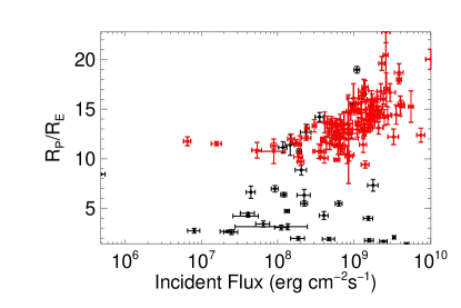
Figure 14.— Top: All planets with measured mass, radius, and incident flux, as listed in exoplanets.org (see Table 4). The black points are planets with $M_{\rm P}<150M_{\earth}$, and the red points are planets with $M_{\rm P}$$>$ 150 $M_{\earth}$. For the giant planets, planet radius increases with incident flux. For low-mass planets, incident flux does not correlate with planet radius. This is because planet radius scales with planet mass more strongly than with incident flux for low-mass planets, whereas incident flux is the primary factor in determining the radii of high-mass planets (see Equation 9). Bottom: Planet radius, divided by dependence on planet mass according to Equation 8, versus incident flux $\text{for }M_{\rm P}<150M_{\earth}$. The best fit to the data suggests a slight trend toward lower radius at higher incident flux, although the data are also consistent with no correlation between incident flux and planet radius.

7.1. Interpretation of the Radius-Mass-Incident Flux Relations

We consider the KOI-94 system in the context of other planets with published values for both mass and radius. We quantify these trends in two fundamental planes (see Equations 8$-$9) for exoplanets that relate their mass, incident flux, and radius from a few Earth masses up to ten Jupiter masses. These equations demonstrate that for low-mass planets, mass is much more important than flux in predicting a planet’s radius, whereas for high-mass planets, incident flux is more important for predicting the radius of a giant planet than the planet mass.

For low-mass planets, inverting Equation 8 predicts the planet’s mass given its radius and incident flux. The small coefficient for mass $\text{for }M_{\rm P}>150M_{\earth}$ indicates that it is difficult to predict the mass of a giant planet given its radius and incident flux.

The small RMS scatter in radius for giant planets ($\delta R_{\rm P}=1.15$ $R_{\earth}$) compared to the typical uncertainty in radius ($\sigma_{R_{\rm P}}=0.76R_{\earth}$) suggests that our model of mass and incident flux affecting the radius of giant planets is appropriate and that other factors, such as orbital period and metallicity, play a small part, if any.

For low-mass planets, the high RMS scatter ($\delta R_{\rm P}=1.41$ $R_{\earth}$) compared to uncertainties in the radius ($\sigma_{R_{\rm P}}=0.34R_{\earth}$) indicates that additional physics might play a role in determining radius. In particular, the composition of low-mass planets could strongly affect planetary radius. Planets on the low-mass branch could have compositions ranging from mostly hydrogen/helium (e.g. Saturn) to mostly water (Charbonneau et al. 2009, e.g. GJ 1214 b) to mostly rock (Batalha et al. 2011, e.g. Kepler 10b). The equations of state of these materials are quite different, allowing a planet of 10$M_{\earth}$ to vary by a factor of 5 in radius depending on its composition, in theory. Despite the potentially large range in compositions at a given mass, the low-mass fundamental plane works reasonably well: extrapolating this relation to Earth, we predict $R_{\rm P}=1.15R_{\earth}$.

Planetary composition might be described in part by the mass-radius relation. For low-mass planets, the exponential dependence of $R_{\rm P}$ on $M_{\rm P}$ is higher than expected. For a body of constant density (for instance, a rocky planet, if we ignore compressibility), we expect $R_{\rm P}\propto M_{\rm P}^{1/3}$. For low-mass planets, the observed relation, $R_{\rm P}\propto M_{\rm P}^{0.52}$, is steeper. This steep increase in radius with mass cannot be explained by the compressibility of material, since compressibility would cause less increase in radius with increasing mass. The extra increase in radius per unit mass suggests a compositional gradient. Within the low-mass regime ($M_{\rm P}<150M_{\earth}$), higher-mass planets might have an increased admixture of volatiles. This is supported by observations in our own solar system; Uranus, Neptune and Saturn have a larger fraction of volatiles than Earth and Venus.

In the giant planet population ($M_{\rm P}$$>$ 150 $M_{\earth}$), the decline in radius with increasing mass corresponds to the onset of electron degeneracy as an important component of the planet’s pressure along with Coulomb forces. For a body supported by electron degeneracy pressure, we expect $R_{\rm P}$ $\propto$ $M_{\rm P}$^-1/3. The dependence of $R_{\rm P}$ $\propto$ $M_{\rm P}$^-0.04, which is measured with a significance of $4\sigma$, indicates that Coulomb forces still play a significant role in supporting high-mass planets.

In planetary modeling, 150 $M_{\earth}$ occurs where the mass-radius relation for model planets (e.g. Fortney et al. 2007) begins to gradually flatten out. It is marked by waning relative importance of electrostatic forces which alone lead to $R\sim M^{1/3}$, and the gradual onset of degeneracy pressure, which for complete degeneracy leads to $R\sim M^{-1/3}$. In an approximate way, 150 $M_{\earth}$ can be thought of as the start of the broad maximum in this curve that leads to radius being nearly independent of mass for giant planets and brown dwarfs (Zapolsky & Salpeter 1969).

The reversal of the correlation between $R_{\rm P}$ and $F$ at 150 $M_{\earth}$ is an interesting feature of the exoplanet population. The current population of observed planets can be sculpted to some degree by evaporative mass loss (Baraffe et al. 2004, 2006; Hubbard et al. 2007; Lopez et al. 2012). X-ray and UV (XUV) photons can drive mass-loss of hydrogen/helium planetary atmospheres, and in the energy-limited escape model (e.g., Erkaev et al. 2007), the mass loss rate depends inversely on the planet density and linearly with the incident XUV flux. Planets with masses near $\sim$150 $M_{\earth}$ are those that have low bulk densities (see Figure 12) are and generally more susceptible to atmospheric mass loss. Under extreme XUV irradiation, some rare planets may migrate from just above 150 $M_{\earth}$ to below.

Unlike the incident flux on a planet, the orbital period of a planet does not correlate with planet radius. This suggests that the mechanism that maintains the inflated radii of giant planets is driven by the incident flux rather than by tidal forces via eccentricity damping. However, because the eccentricities of many planets are poorly constrained, it is difficult to calculate the tidal power deposited in the planet. The uncertainty in the heat dissipation timescale further complicates our analysis, since we cannot determine how long ago various planets might have been in sufficiently eccentric orbits for tidal forcing to inflate them. Regardless, a planet’s radius is more strongly correlated with the incident flux it receives than its orbital period. Future studies of warm Jupiters and hot Jupiters with various orbital periods and eccentricities will help elucidate the role of potential interior heating mechanisms. However, the goodness of fit between the radius, mass, and incident flux for giant planets suggests that the current role of tidal heating (or any other inflation mechanism that is not driven by incident flux) is quite small.

There are only 9 low-mass planets out of 35 that receive more than the median incident flux and 9 that have shorter than the median orbital period, whereas the population of giant planets is more evenly split. Howard et al. (2012) find that the occurrence of giant planets is smaller than the occurrence of small planets at orbital periods less than 10 days, suggesting that the hot Jupiters in this work are over-represented. The over-abundance of hot Jupiters compared to hot Neptunes in this sample could be due to historic observational bias of hot Jupiters, since the detection of Neptune-size and smaller planets from the ground was infrequent before the Kepler Mission. Measuring the masses of Neptune-size and smaller planets that receive high incident flux is necessary to probe the radius-mass-incident flux relation for low-mass planets.

7.2. Comparison to Previous Work

The idea of searching for correlations between planetary radius, mass, incident flux, and other measurable planetary and stellar parameters is not novel; as mentioned in §1, Enoch et al. (2012) and Kane & Gelino (2012) sought empirical relations between the properties of planets and their host stars. Here, we incorporate an additional year’s worth of planet discoveries and mass determinations, especially for Kepler planets. There are additional differences between our work and theirs, and we highlight how this study differs from previous work.

The primary difference between Enoch et al. (2012) and the work presented here is that Enoch et al. (2012) study 16 planets within orbital periods of 10 days and with masses between 0.1 and 0.5 $M_{\rm J}$, whereas here we study 35 planets with masses below 150 $M_{\earth}$ (0.5 $M_{\rm J}$). Whereas Enoch et al. (2012) consider three mass regimes of planets ($0.1<M_{\rm P}<0.5M_{\rm J}$, $0.5M_{\rm J}<M_{\rm P}<2.0M_{\rm J}$, $2.0M_{\rm J}<M_{\rm P}<12M_{\rm J}$), here, we only consider two regimes ($M_{\rm P}<150M_{\earth}$, $150M_{\earth}<M_{\rm P}<13M_{\rm J}$). With the additional transiting planets included here, we do not see evidence for three mass domains.

However, we find that fits to the data incorporating only mass and incident flux predict the radius of a planet as well as the fits described in Enoch et al. (2012). Enoch et al. (2012) find an average absolute deviation in the predicted radius from the true radius of 0.11 $R_{\rm J}$ (1.23 $R_{\earth}$) across all three of their mass regimes, whereas we find a mean absolute difference of 1.41 $\text{for }M_{\rm P}<150M_{\earth}$and 1.15 $\text{for }M_{\rm P}>150M_{\earth}$, or 1.23 $R_{\earth}$, over the whole sample. Incorporating the orbital period of the planet, the stellar metallicity, and the stellar age does not significantly improve the accuracy of the predicted planetary radius.

The slope of the mass-radius fit for $M_{\rm P}<150M_{\earth}$ reported here, $0.53~{}\pm 0.0052$, is only 1.5$\sigma$ different from the value of 0.45 reported in Enoch et al. (2012) for planets with $M_{\rm P}<0.5M_{\rm J}$. Our slope of the mass-radius fit for the high-mass planets, $-0.039~{}$, falls between the values for middle- and high-mass regimes in Enoch et al. (2012), 0 and -0.09.

Kane & Gelino (2012) used a similar prescription to our method to obtain a mass-radius relation. They fit a power law between the mass and radius of low-mass planets. However, they assumed that giant planet radius was constant with planet mass (at one Jupiter radius). Furthermore, they did not consider the effects of incident flux on planetary radius in either mass regime.

8. Conclusions

1. The KOI-94 system In this paper, we presented 26 radial velocity measurements of KOI-94 obtained on Keck/HIRES. These measurements confirm the giant planet KOI-94d and strongly support the existence of other transiting planets in the system.

   1. Properties of Planet KOI-94d The mass is $106\pm 11$$M_{\earth}$. The radius is $11.27\pm 1.06$$R_{\earth}$. The density is $0.363\pm 0.101$$\rm g\,cm^{-3}$. The planet is enriched in metals by a factor of $11\pm 4$ with respect to the parent star. The mass of heavy elements, or “metals,” in the planet is $18\pm 6$ $M_{\earth}$.

   2. Properties of Planets KOI-94b, KOI-94c, KOI-94e These planets were detected at significance of less than $3\sigma$ in the radial velocity data. The radial velocity detections of planets e and b are marginal ($>2\sigma$), whereas the radial velocity measurements of planet c are consistent with a non-detection to $1\sigma$. More RVs and a numerical analysis of the TTVs are needed to better characterize these planets. However, the TTVs, multiplicity of the system, lack of evidence for another star, RM effect during the transit of KOI-94d  and coplanarity of these objects strongly suggest that these candidates are planets.

   3. Dynamical Stability of the KOI-94 System The system is dynamically stable on a 1 Myr timescale for a variety of configurations, including circular orbital solutions. Although some eccentric solutions are stable, the best-fit solution considered in this work is unstable due to close encounters of planets b and c.

   4. No Massive Outer Perturbers The non-detection of a trend in radial velocity, the lack of spectral features from a second star to 1% of the brightness of KOI-94within 0.4″, and the non-detection of a companion outside 0.5″(in both AO and speckle imaging) rule out large, outer companions.

2. Radius-Mass-Incident Flux Relation Using the KOI-94 system and other exoplanets (138 exoplanets total) with published values and uncertainties for planet mass, radius, and incident flux, we establish two fundamental planes for exoplanets that relate planet radius, planet mass, and incident flux between 2 and 3000 $M_{\earth}$ in Equations 8$-$11. The slope of the mass-radius relation for low-mass planets suggests that as low-mass planets increase in mass, the admixture of volatiles increases. Although the plane for $\text{for }M_{\rm P}>150M_{\earth}$ fits the giant planets very well, a higher RMS compared to uncertainties in radius ($~{}400\%$) for the low-mass planets suggests that additional physics, such as the composition of heavy elements, might contribute to the radii of these planets.

Appendix A Long Tables

Table 3Star and planet parameters for the KOI-94 system.

Parameter	Value	Notes
Transit and orbital parameters: KOI-94b
Orbital period $P$ (days)	$3.743208\pm 0.000015$	A
Midtransit time $E$ (BJD)	$2454964.6175\pm 0.0021$	A
Scaled semimajor axis $a/R_{\star}$	$7.25\pm 0.59$	A
Scaled planet radius $R_{\rm P}$/$R_{\star}$	$0.01031\pm 0.00014$	A
Impact parameter $b$	$0.088\pm 0.072$	A
Orbital inclination $i$ (deg)	$89.30\pm 0.57$	A
Orbital semi-amplitude $K$ ($\rm m\,s^{-1}$)	$3.3\pm 1.4$	B
Orbital eccentricity $e$	$0.25\pm 0.17$	B
Center-of-mass velocity $\gamma$ ($\rm m\,s^{-1}$)	$2.1\pm 1.4$	B
Transit and orbital parameters: KOI-94c
Orbital period $P$ (days)	$10.423648\pm 0.000016$	A
Midtransit time $E$ (BJD)	$2454971.00870\pm 0.00103$	A
Scaled semimajor axis $a/R_{\star}$	$14.3\pm 1.2$	A
Scaled planet radius $R_{\rm P}$/$R_{\star}$	$0.02599\pm 0.00047$	A
Impact parameter $b$	$0.41\pm 0.018$	A
Orbital inclination $i$ (deg)	$88.36\pm 0.75$	A
Orbital semi-amplitude $K$ ($\rm m\,s^{-1}$)	$3.5^{+1.3}_{-3.5}$	B
Orbital eccentricity $e$	$0.43\pm 0.23$	B
Transit and orbital parameters: KOI-94d
Orbital period $P$ (days)	$22.3429890\pm 0.0000067$	A
Midtransit time $E$ (BJD)	$2454965.74052\pm 0.00015$	A
Scaled semimajor axis $a/R_{\star}$	$23.8\pm 1.9$	A
Scaled planet radius $R_{\rm P}$/$R_{\star}$	$0.068016\pm 0.000080$	A
Impact parameter $b$	$0.055\pm 0.051$	A
Orbital inclination $i$ (deg)	$89.871\pm 0.123$	A
Orbital semi-amplitude $K$ ($\rm m\,s^{-1}$)	$18.3\pm 1.5$	B
Orbital eccentricity $e$	$0.022\pm 0.038$	B
Transit and orbital parameters: KOI-94e
Orbital period $P$ (days)	$54.32031\pm 0.00012$	A
Midtransit time $E$ (BJD)	$2454994.2379\pm 0.0012$	A
Scaled semimajor axis $a/R_{\star}$	$43.1\pm 3.5$	A
Scaled planet radius $R_{\rm P}$/$R_{\star}$	$0.03960\pm 0.00024$	A
Impact parameter $b$	$0.18\pm 0.11$	A
Orbital inclination $i$ (deg)	$89.76\pm 0.15$	A
Orbital semi-amplitude $K$ ($\rm m\,s^{-1}$)	$4.5^{+2.3}_{-3.5}$	B
Orbital eccentricity $e$	$0.019\pm 0.23$	B
Observed stellar parameters
Effective temperature $T_{\rm eff}$(K)	$6182\pm 58$	C
Spectroscopic gravity $\log{g}$(cgs)	$4.181\pm 0.066$	C
Metallicity [Fe/H]	$+0.0228\pm 0.0020$	C
Projected rotation $v\sin{i}$($\rm km\,s^{-1}$)	$7.3\pm 0.5$	C
Fundamental Stellar Properties
Mass $M_{\star}$($M_{\sun}$)	$1.277\pm 0.050$	D
Radius $R_{\star}$($R_{\sun}$)	$1.52\pm 0.14$	D
Surface gravity $\log{g}_{\star}$ (cgs)	$4.181\pm 0.066$	D
Luminosity $L_{\star}$ ($L_{\sun}$)	$3.01\pm 0.60$	D
Kepler Magnitude $K_{p}$ (mag)	$12.2$	D
Age (Gyr)	$3.16\pm 0.39$	D
Planetary parameters: KOI-94b
Mass $M_{\rm P}$ ($M_{\earth}$)	$10.5\pm 4.6$	B,C,D
Radius $R_{\rm P}$ ($R_{\earth}$)	$1.71\pm 0.16$	A,B,C,D
Density $\rho_{\rm P}$ ($\rm g\,cm^{-3}$)	$10.1\pm 5.5$	A,B,C,D
Orbital semi-major axis $a$ (AU)	$0.05119\pm 0.00067$	E
Incident Flux $F$ ($\rm erg\,s^{-1}\,cm^{-2}$)	$1.58\times 10^{9}$	A,C
Equilibrium temperature $T_{\rm eq}$ (K)	$1486$	F
Planetary parameters: KOI-94c
Mass $M_{\rm P}$ ($M_{\earth}$)	$15.6^{+5.7}_{-15.6}$	B,C,D
Radius $R_{\rm P}$ ($R_{\earth}$)	$4.32\pm 0.41$	A,B,C,D
Density $\rho_{\rm P}$ ($\rm g\,cm^{-3}$)	$0.91^{+0.36}_{-0.91}$	A,B,C,D
Orbital semi-major axis $a$ (AU)	$0.1013\pm 0.0013$	E
Incident Flux $F$ ($\rm erg\,s^{-1}\,cm^{-2}$)	$4.03\times 10^{8}$	A,C
Equilibrium temperature $T_{\rm eq}$ (K)	$1012$	F
Planetary parameters: KOI-94d
Mass $M_{\rm P}$ ($M_{\earth}$)	$106\pm 11$	B,C,D
Radius $R_{\rm P}$ ($R_{\earth}$)	$11.27\pm 1.06$	A,B,C,D
Density $\rho_{\rm P}$ ($\rm g\,cm^{-3}$)	$0.363\pm 0.101$	A,B,C,D
Orbital semi-major axis $a$ (AU)	$0.1684\pm 0.0022$	E
Incident Flux $F$ ($\rm erg\,s^{-1}\,cm^{-2}$)	$1.46\times 10^{8}$	A,C
Equilibrium temperature $T_{\rm eq}$ (K)	$806$	F
Planetary parameters: KOI-94e
Mass $M_{\rm P}$ ($M_{\earth}$)	$35^{+18}_{-28}$	B,C,D
Radius $R_{\rm P}$ ($R_{\earth}$)	$6.56\pm 0.62$	A,B,C,D
Density $\rho_{\rm P}$ ($\rm g\,cm^{-3}$)	$0.60^{+0.26}_{-0.56}$	A,B,C,D
Orbital semi-major axis $a$ (AU)	$0.3046\pm 0.0040$	E
Incident Flux $F$ ($\rm erg\,s^{-1}\,cm^{-2}$)	$4.46\times 10^{8}$	A,C
Equilibrium temperature $T_{\rm eq}$ (K)	$584$	F

Note. — A: Based primarily on an analysis of the photometry,

B: Based on a joint analysis of the photometry and radial velocities,

C: Based on an analysis by D. Fischer of the Keck/HIRES template spectrum using SME (Valenti & Piskunov 1996),

D: Based on the Yale-Yonsei isochrones (Yi et al. 2001) and the results from A, B, and C,

E: Based on Newton’s revised version of Kepler’s Third Law and the results from D,

F: Calculated assuming Bond albedos of 0.3 (b; Earth), 0.4 (c; Neptune), 0.34 (d; Jupiter), and 0.4 (e; Neptune) and complete redistribution of heat for reradiation.

Table 4Exoplanets with Measured Mass and Radius

Name	$M_{\rm P}$	$R_{\rm P}$	Incident Flux	Period	First Ref.	Orbit Ref.
	($M_{\earth}$)	($R_{\earth}$)	($\rm erg\,s^{-1}\,cm^{-2}$)	(days)
55 Cnc e	7.862	2.078	3.34E+09	0.737	McArthur et al. (2004)	Demory et al. (2011)
CoRoT-1 b	327.284	16.685	2.96E+09	1.509	Barge et al. (2008)	Barge et al. (2008)
CoRoT-10 b	875.699	10.862	5.39E+07	13.241	Bonomo et al. (2010)	Bonomo et al. (2010)
CoRoT-11 b	746.274	16.013	2.04E+09	2.994	Gandolfi et al. (2010)	Gandolfi et al. (2010)
CoRoT-12 b	292.131	16.125	9.86E+08	2.828	Gillon et al. (2010)	Gillon et al. (2010)
CoRoT-13 b	416.654	9.910	5.99E+08	4.035	Cabrera et al. (2010)	Cabrera et al. (2010)
CoRoT-14 b	2445.485	12.205	3.29E+09	1.512	Tingley et al. (2011)	Tingley et al. (2011)
CoRoT-17 b	781.832	11.422	1.32E+09	3.768	Csizmadia et al. (2011)	Csizmadia et al. (2011)
CoRoT-18 b	1108.075	14.669	1.23E+09	1.900	Hébrard et al. (2011)	Hébrard et al. (2011)
CoRoT-19 b	352.115	14.445	1.72E+09	3.897	Guenther et al. (2012)	Guenther et al. (2012)
CoRoT-2 b	1041.197	16.405	1.27E+09	1.743	Alonso et al. (2008)	Alonso et al. (2008)
CoRoT-4 b	228.008	13.325	3.02E+08	9.202	Moutou et al. (2008); Aigrain et al. (2008)	Moutou et al. (2008)
CoRoT-5 b	147.002	15.542	9.74E+08	4.038	Rauer et al. (2009)	Rauer et al. (2009)
CoRoT-6 b	938.715	13.057	2.43E+08	8.887	Fridlund et al. (2010)	Fridlund et al. (2010)
CoRoT-7 b	5.021	1.677	2.43E+09	0.854	Queloz et al. (2009); Léger et al. (2009)	Queloz et al. (2009)
CoRoT-8 b	68.673	6.383	1.21E+08	6.212	Bordé et al. (2010)	Bordé et al. (2010)
CoRoT-9 b	268.099	11.758	6.59E+06	95.274	Deeg et al. (2010)	Deeg et al. (2010)
GJ 1214 b	6.468	2.675	2.23E+07	1.580	Charbonneau et al. (2009)	Carter et al. (2011)
GJ 436 b	23.105	4.218	4.09E+07	2.644	Butler et al. (2004)	Maness et al. (2007)
HAT-P-1 b	169.196	13.908	6.58E+08	4.465	Bakos et al. (2007a)	Bakos et al. (2007a)
HAT-P-11 b	26.231	4.725	1.33E+08	4.888	Bakos et al. (2010)	Bakos et al. (2010)
HAT-P-12 b	66.997	10.739	1.91E+08	3.213	Hartman et al. (2009)	Hartman et al. (2009)
HAT-P-13 b	272.394	14.344	1.67E+09	2.916	Bakos et al. (2009b)	Winn et al. (2010)
HAT-P-14 b	710.648	12.877	1.37E+09	4.628	Torres et al. (2010)	Torres et al. (2010)
HAT-P-15 b	620.231	12.004	1.51E+08	10.864	Kovács et al. (2010)	Kovács et al. (2010)
HAT-P-16 b	1335.623	14.434	1.58E+09	2.776	Buchhave et al. (2010)	Buchhave et al. (2010)
HAT-P-17 b	168.493	11.310	8.91E+07	10.339	Howard et al. (2012)	Howard et al. (2012)
HAT-P-18 b	62.675	11.142	1.17E+08	5.508	Hartman et al. (2011a)	Hartman et al. (2011a)
HAT-P-19 b	92.889	12.676	2.36E+08	4.009	Hartman et al. (2011a)	Hartman et al. (2011a)
HAT-P-2 b	2819.241	12.956	1.10E+09	5.633	Bakos et al. (2007c)	Pál et al. (2010)
HAT-P-20 b	2316.734	9.708	2.02E+08	2.875	Bakos et al. (2011)	Bakos et al. (2011)
HAT-P-21 b	1296.160	11.466	6.12E+08	4.124	Bakos et al. (2011)	Bakos et al. (2011)
HAT-P-22 b	683.741	12.094	6.12E+08	3.212	Bakos et al. (2011)	Bakos et al. (2011)
HAT-P-23 b	666.163	15.318	4.03E+09	1.213	Bakos et al. (2011)	Bakos et al. (2011)
HAT-P-24 b	217.977	13.908	1.63E+09	3.355	Kipping et al. (2010)	Kipping et al. (2010)
HAT-P-26 b	18.640	6.327	2.23E+08	4.235	Hartman et al. (2011b)	Hartman et al. (2011b)
HAT-P-27 b	195.955	11.623	4.34E+08	3.040	Anderson et al. (2011b)	Anderson et al. (2011b)
HAT-P-28 b	199.536	13.572	8.27E+08	3.257	Buchhave et al. (2011a)	Buchhave et al. (2011a)
HAT-P-29 b	247.580	12.396	5.70E+08	5.723	Buchhave et al. (2011a)	Buchhave et al. (2011a)
HAT-P-3 b	189.327	10.067	4.08E+08	2.900	Torres et al. (2007)	Torres et al. (2008)
HAT-P-30 b	225.996	15.005	1.63E+09	2.811	Johnson et al. (2011)	Johnson et al. (2011)
HAT-P-31 b	689.358	11.982	8.46E+08	5.005	Kipping et al. (2011)	Kipping et al. (2011)
HAT-P-32 b	302.182	22.810	2.62E+09	2.150	Hartman et al. (2011c)	Hartman et al. (2011c)
HAT-P-33 b	243.556	20.458	2.60E+09	3.474	Hartman et al. (2011c)	Hartman et al. (2011c)
HAT-P-34 b	1059.600	13.404	7.35E+08	5.453	Bakos et al. (2012)	Bakos et al. (2012)
HAT-P-35 b	335.047	14.915	1.41E+09	3.647	Bakos et al. (2012)	Bakos et al. (2012)
HAT-P-36 b	584.539	14.154	2.49E+09	1.327	Bakos et al. (2012)	Bakos et al. (2012)
HAT-P-37 b	372.996	13.191	6.01E+08	2.797	Bakos et al. (2012)	Bakos et al. (2012)
HAT-P-4 b	213.416	14.266	1.87E+09	3.057	Kovács et al. (2007)	Kovács et al. (2007)
HAT-P-5 b	335.490	14.042	1.27E+09	2.788	Bakos et al. (2007b)	Bakos et al. (2007b)
HAT-P-6 b	336.749	14.893	1.78E+09	3.853	Noyes et al. (2008)	Noyes et al. (2008)
HAT-P-7 b	572.656	15.262	5.57E+09	2.205	Pál et al. (2008)	Winn et al. (2009)
HAT-P-8 b	411.052	16.797	2.24E+09	3.076	Latham et al. (2009)	Latham et al. (2009)
HAT-P-9 b	246.817	15.677	1.24E+09	3.923	Shporer et al. (2009)	Shporer et al. (2009)
HD 149026 b	114.882	7.323	1.78E+09	2.876	Sato et al. (2005)	Carter et al. (2009)
HD 17156 b	1049.670	11.422	1.95E+08	21.217	Fischer et al. (2007)	Barbieri et al. (2009)
HD 189733 b	363.454	12.743	4.71E+08	2.219	Bouchy et al. (2005)	Bouchy et al. (2005)
HD 209458 b	219.181	15.218	9.93E+08	3.525	Henry et al. (2000); Charbonneau et al. (2000)	Torres et al. (2008)
HD 80606 b	1236.479	11.522	1.59E+07	111.437	Naef et al. (2001)	Moutou et al. (2009)
KOI-135 b	1027.001	13.437	1.63E+09	3.024	Borucki et al. (2011)	Bonomo et al. (2012)
KOI-196 b	156.857	9.417	1.40E+09	1.856	Borucki et al. (2011)	Santerne et al. (2011)
KOI-204 b	324.519	13.885	1.51E+09	3.247	Borucki et al. (2011)	Bonomo et al. (2012)
KOI-254 b	162.563	10.750	8.91E+07	2.455	Borucki et al. (2011)	Johnson et al. (2012)
KOI-428 b	691.836	13.101	1.54E+09	6.873	Santerne et al. (2011)	Santerne et al. (2011)
Kepler-10 b	4.539	1.415	4.88E+09	0.837	Batalha et al. (2011)	Batalha et al. (2011)
Kepler-11 b	4.298	1.968	1.86E+08	10.304	Lissauer et al. (2011)	Lissauer et al. (2011)
Kepler-11 c	13.500	3.147	1.36E+08	13.025	Lissauer et al. (2011)	Lissauer et al. (2011)
Kepler-11 d	6.100	3.427	6.50E+07	22.687	Lissauer et al. (2011)	Lissauer et al. (2011)
Kepler-11 e	8.401	4.515	4.11E+07	31.996	Lissauer et al. (2011)	Lissauer et al. (2011)
Kepler-11 f	2.298	2.607	2.48E+07	46.689	Lissauer et al. (2011)	Lissauer et al. (2011)
Kepler-12 b	137.283	18.980	1.09E+09	4.438	Borucki et al. (2011)	Fortney et al. (2011)
Kepler-14 b	2671.703	12.721	1.32E+09	6.790	Borucki et al. (2011)	Buchhave et al. (2011b)
Kepler-15 b	210.532	10.750	3.45E+08	4.943	Borucki et al. (2011)	Endl et al. (2011)
Kepler-16 b	105.833	8.441	4.84E+05	228.776	Borucki et al. (2011)	Doyle et al. (2011)
Kepler-17 b	788.004	14.893	2.10E+09	1.486	Borucki et al. (2011)	Désert et al. (2011)
Kepler-18 b	6.900	5.484	6.32E+08	3.505	Borucki et al. (2011)	Cochran et al. (2011)
Kepler-18 c	17.299	5.484	2.24E+08	7.642	Borucki et al. (2011)	Cochran et al. (2011)
Kepler-18 d	16.399	6.973	9.21E+07	14.859	Borucki et al. (2011)	Cochran et al. (2011)
Kepler-20 b	8.474	1.906	4.70E+08	3.696	Borucki et al. (2011)	Gautier et al. (2012b)
Kepler-20 c	15.734	3.064	1.12E+08	10.854	Borucki et al. (2011)	Gautier et al. (2012b)
Kepler-20 d	7.528	2.745	8.12E+06	77.612	Borucki et al. (2011)	Gautier et al. (2012b)
Kepler-4 b	24.544	3.998	1.54E+09	3.213	Borucki et al. (2010)	Borucki et al. (2010)
Kepler-5 b	672.699	16.024	2.42E+09	3.548	Koch et al. (2010)	Koch et al. (2010)
Kepler-6 b	212.739	14.815	1.16E+09	3.235	Dunham et al. (2010)	Dunham et al. (2010)
Kepler-7 b	139.127	16.550	1.33E+09	4.886	Latham et al. (2010)	Latham et al. (2010)
Kepler-8 b	186.158	15.890	1.73E+09	3.523	Jenkins et al. (2010)	Jenkins et al. (2010)
OGLE-TR-182 b	325.603	12.653	7.45E+08	3.979	Pont et al. (2008)	Pont et al. (2008)
OGLE-TR-211 b	240.675	15.229	2.01E+09	3.677	Udalski et al. (2008)	Udalski et al. (2008)
OGLE2-TR-L9 b	1453.828	18.028	3.89E+09	2.486	Snellen et al. (2009)	Snellen et al. (2009)
Qatar-1 b	346.352	13.034	8.45E+08	1.420	Alsubai et al. (2011)	Alsubai et al. (2011)
TrES-1 b	239.152	11.948	3.88E+08	3.030	Alonso et al. (2004)	Alonso et al. (2004)
TrES-2 b	381.607	13.706	1.14E+09	2.471	O’Donovan et al. (2006)	O’Donovan et al. (2006)
TrES-4 b	292.473	19.607	2.31E+09	3.554	Mandushev et al. (2007)	Mandushev et al. (2007)
TrES-5 b	565.109	13.538	1.09E+09	1.482	Mandushev et al. (2011)	Mandushev et al. (2011)
WASP-1 b	263.078	16.976	2.65E+09	2.520	Collier Cameron et al. (2007)	Simpson et al. (2011a)
WASP-10 b	1013.770	12.094	2.38E+08	3.093	Christian et al. (2009)	Christian et al. (2009)
WASP-11 b	171.543	10.190	1.87E+08	3.722	West et al. (2009b); Bakos et al. (2009a)	West et al. (2009b)
WASP-12 b	432.432	20.044	1.01E+10	1.091	Hebb et al. (2009)	Maciejewski et al. (2011)
WASP-13 b	152.357	15.554	1.12E+09	4.353	Skillen et al. (2009)	Skillen et al. (2009)
WASP-14 b	2444.754	14.344	2.75E+09	2.244	Joshi et al. (2009)	Joshi et al. (2009)
WASP-15 b	172.613	15.990	1.69E+09	3.752	West et al. (2009a)	West et al. (2009a)
WASP-16 b	267.695	11.287	6.64E+08	3.119	Lister et al. (2009)	Lister et al. (2009)
WASP-17 b	156.828	16.909	1.34E+09	3.735	Anderson et al. (2010)	Anderson et al. (2010)
WASP-18 b	3206.179	12.385	7.50E+09	0.941	Hellier et al. (2009b)	Hellier et al. (2009b)
WASP-19 b	360.211	15.520	4.13E+09	0.789	Hebb et al. (2010)	Hellier et al. (2011)
WASP-2 b	288.782	11.993	6.47E+08	2.152	Collier Cameron et al. (2007)	Charbonneau et al. (2007)
WASP-21 b	95.431	11.982	5.75E+08	4.322	Bouchy et al. (2010)	Bouchy et al. (2010)
WASP-22 b	177.678	12.541	9.25E+08	3.533	Maxted et al. (2010a)	Maxted et al. (2010a)
WASP-23 b	277.208	10.772	3.69E+08	2.944	Triaud et al. (2011)	Triaud et al. (2011)
WASP-24 b	346.738	14.557	2.22E+09	2.341	Street et al. (2010)	Simpson et al. (2011a)
WASP-25 b	183.847	13.661	5.06E+08	3.765	Enoch et al. (2011)	Enoch et al. (2011)
WASP-26 b	323.366	14.781	9.03E+08	2.757	Smalley et al. (2010)	Smalley et al. (2010)
WASP-29 b	77.261	8.869	2.04E+08	3.923	Hellier et al. (2010)	Hellier et al. (2010)
WASP-3 b	639.396	14.445	3.56E+09	1.847	Pollacco et al. (2008)	Tripathi et al. (2010)
WASP-31 b	152.339	17.211	1.40E+09	3.406	Anderson et al. (2011a)	Anderson et al. (2011a)
WASP-32 b	1129.221	13.213	1.35E+09	2.719	Maxted et al. (2010b)	Maxted et al. (2010b)
WASP-34 b	185.399	13.661	4.13E+08	4.318	Smalley et al. (2011)	Smalley et al. (2011)
WASP-35 b	227.906	14.781	1.01E+09	3.162	Enoch et al. (2011)	Enoch et al. (2011)
WASP-36 b	721.220	14.210	1.89E+09	1.537	Smith et al. (2012)	Smith et al. (2012)
WASP-37 b	570.041	12.989	7.01E+08	3.577	Simpson et al. (2011b)	Simpson et al. (2011b)
WASP-38 b	854.794	12.250	5.49E+08	6.872	Barros et al. (2011)	Barros et al. (2011)
WASP-39 b	90.367	14.221	3.54E+08	4.055	Faedi et al. (2011)	Faedi et al. (2011)
WASP-4 b	388.827	15.352	1.77E+09	1.338	Wilson et al. (2008)	Wilson et al. (2008)
WASP-41 b	296.362	13.437	5.35E+08	3.052	Maxted et al. (2011)	Maxted et al. (2011)
WASP-43 b	564.470	10.414	8.11E+08	0.813	Hellier et al. (2011)	Hellier et al. (2011)
WASP-48 b	312.807	18.700	3.88E+09	2.144	Enoch et al. (2011)	Enoch et al. (2011)
WASP-5 b	516.398	13.112	2.09E+09	1.628	Anderson et al. (2008)	Anderson et al. (2008)
WASP-50 b	467.967	12.911	8.54E+08	1.955	Gillon et al. (2011)	Gillon et al. (2011)
WASP-6 b	165.697	13.706	4.46E+08	3.361	Gillon et al. (2009)	Gillon et al. (2009)
WASP-7 b	292.162	10.246	8.60E+08	4.955	Hellier et al. (2009a)	Hellier et al. (2009a)
WASP-8 b	679.482	11.623	1.76E+08	8.159	Queloz et al. (2010)	Queloz et al. (2010)
XO-1 b	291.903	13.504	4.82E+08	3.942	McCullough et al. (2006)	McCullough et al. (2006)
XO-2 b	180.056	11.007	6.93E+08	2.616	Burke et al. (2007)	Burke et al. (2007)
XO-5 b	366.286	11.534	4.82E+08	4.188	Burke et al. (2008)	Burke et al. (2008)
KOI-94 b	9.400	1.770	1.58E+09	3.743	Borucki et al. (2011)	Weiss et al. (2013)
KOI-94 c	8.300	4.280	4.03E+08	10.424	Borucki et al. (2011)	Weiss et al. (2013)
KOI-94 d	105.000	11.400	1.46E+08	22.343	Borucki et al. (2011)	Weiss et al. (2013)
KOI-94 e	38.000	6.640	4.46E+07	54.320	Batalha et al. (2012)	Weiss et al. (2013)
Earth	1.000	1.000	1.07E+06	365.250
Jupiter	317.817	11.198	3.97E+04	4336.069
Saturn	95.027	9.440	1.17E+04	10833.641
Uranus	14.535	4.003	2.91E+03	30730.951
Neptune	17.147	3.879	1.19E+03	60157.796

References

- Adams et al. (2012) Adams, E. R., Ciardi, D. R., Dupree, a. K., et al. 2012, The Astronomical Journal, 144, 42
- Aigrain et al. (2008) Aigrain, S., Collier Cameron, A., Ollivier, M., et al. 2008, A&A, 488, L43
- Albrecht et al. (2013) Albrecht, S., Winn, J. N., Marcy, G. W., et al. 2013, ArXiv e-prints
- Alonso et al. (2004) Alonso, R., Brown, T. M., Torres, G., et al. 2004, ApJ, 613, L153
- Alonso et al. (2008) Alonso, R., Auvergne, M., Baglin, A., et al. 2008, A&A, 482, L21
- Alsubai et al. (2011) Alsubai, K. A., Parley, N. R., Bramich, D. M., et al. 2011, MNRAS, 417, 709
- Anderson et al. (2008) Anderson, D. R., Gillon, M., Hellier, C., et al. 2008, MNRAS, 387, L4
- Anderson et al. (2010) Anderson, D. R., Hellier, C., Gillon, M., et al. 2010, ApJ, 709, 159
- Anderson et al. (2011a) Anderson, D. R., Collier Cameron, A., Hellier, C., et al. 2011a, A&A, 531, A60
- Anderson et al. (2011b) Anderson, D. R., Barros, S. C. C., Boisse, I., et al. 2011b, PASP, 123, 555
- Arras & Socrates (2010) Arras, P., & Socrates, A. 2010, ApJ, 714, 1
- Bakos et al. (2007a) Bakos, G. Á., Noyes, R. W., Kovács, G., et al. 2007a, ApJ, 656, 552
- Bakos et al. (2007b) Bakos, G. Á., Shporer, A., Pál, A., et al. 2007b, ApJ, 671, L173
- Bakos et al. (2007c) Bakos, G. Á., Kovács, G., Torres, G., et al. 2007c, ApJ, 670, 826
- Bakos et al. (2009a) Bakos, G. Á., Pál, A., Torres, G., et al. 2009a, ApJ, 696, 1950
- Bakos et al. (2009b) Bakos, G. Á., Howard, A. W., Noyes, R. W., et al. 2009b, ApJ, 707, 446
- Bakos et al. (2010) Bakos, G. Á., Torres, G., Pál, A., et al. 2010, ApJ, 710, 1724
- Bakos et al. (2011) Bakos, G. Á., Hartman, J., Torres, G., et al. 2011, ApJ, 742, 116
- Bakos et al. (2012) Bakos, G. Á., Hartman, J. D., Torres, G., et al. 2012, AJ, 144, 19
- Baraffe et al. (2006) Baraffe, I., Alibert, Y., Chabrier, G., & Benz, W. 2006, A&A, 450, 1221
- Baraffe et al. (2010) Baraffe, I., Chabrier, G., & Barman, T. 2010, Reports on Progress in Physics, 73, 016901
- Baraffe et al. (2004) Baraffe, I., Selsis, F., Chabrier, G., et al. 2004, A&A, 419, L13
- Barbieri et al. (2009) Barbieri, M., Alonso, R., Desidera, S., et al. 2009, A&A, 503, 601
- Barge et al. (2008) Barge, P., Baglin, A., Auvergne, M., et al. 2008, A&A, 482, L17
- Barros et al. (2011) Barros, S. C. C., Faedi, F., Collier Cameron, A., et al. 2011, A&A, 525, A54
- Batalha et al. (2011) Batalha, N. M., Borucki, W. J., Bryson, S. T., et al. 2011, ApJ, 729, 27
- Batalha et al. (2012) Batalha, N. M., Rowe, J. F., Bryson, S. T., et al. 2012, ArXiv e-prints
- Batygin & Stevenson (2010) Batygin, K., & Stevenson, D. J. 2010, ApJ, 714, L238
- Bodenheimer et al. (2001) Bodenheimer, P., Lin, D. C. N., & Mardling, R. 2001, The Astrophysical Journal, 10, 466
- Bonomo et al. (2010) Bonomo, A. S., Santerne, A., Alonso, R., et al. 2010, A&A, 520, A65
- Bonomo et al. (2012) Bonomo, A. S., Hébrard, G., Santerne, A., et al. 2012, A&A, 538, A96
- Bordé et al. (2010) Bordé, P., Bouchy, F., Deleuil, M., et al. 2010, A&A, 520, A66
- Borucki et al. (2010) Borucki, W. J., Koch, D. G., Brown, T. M., et al. 2010, ApJ, 713, L126
- Borucki et al. (2011) Borucki, W. J., Koch, D. G., Basri, G., et al. 2011, ApJ, 736, 19
- Borucki et al. (2012) Borucki, W. J., Koch, D. G., Batalha, N., et al. 2012, ApJ, 745, 120
- Bouchy et al. (2005) Bouchy, F., Udry, S., Mayor, M., et al. 2005, A&A, 444, L15
- Bouchy et al. (2010) Bouchy, F., Hebb, L., Skillen, I., et al. 2010, A&A, 519, A98
- Buchhave et al. (2010) Buchhave, L. A., Bakos, G. Á., Hartman, J. D., et al. 2010, ApJ, 720, 1118
- Buchhave et al. (2011a) —. 2011a, ApJ, 733, 116
- Buchhave et al. (2011b) Buchhave, L. A., Latham, D. W., Carter, J. A., et al. 2011b, ApJS, 197, 3
- Burke et al. (2007) Burke, C. J., McCullough, P. R., Valenti, J. A., et al. 2007, ApJ, 671, 2115
- Burke et al. (2008) —. 2008, ApJ, 686, 1331
- Burrows et al. (2007) Burrows, A., Hubeny, I., Budaj, J., & Hubbard, W. B. 2007, ApJ, 661, 502
- Butler et al. (2004) Butler, R. P., Vogt, S. S., Marcy, G. W., et al. 2004, ApJ, 617, 580
- Cabrera et al. (2010) Cabrera, J., Bruntt, H., Ollivier, M., et al. 2010, A&A, 522, A110
- Carter et al. (2009) Carter, J. A., Winn, J. N., Gilliland, R., & Holman, M. J. 2009, ApJ, 696, 241
- Carter et al. (2011) Carter, J. A., Winn, J. N., Holman, M. J., et al. 2011, ApJ, 730, 82
- Chabrier & Baraffe (2007) Chabrier, G., & Baraffe, I. 2007, ApJ, 661, L81
- Chambers (1999) Chambers, J. E. 1999, MNRAS, 304, 793
- Charbonneau et al. (2000) Charbonneau, D., Brown, T. M., Latham, D. W., & Mayor, M. 2000, ApJ, 529, L45
- Charbonneau et al. (2007) Charbonneau, D., Winn, J. N., Everett, M. E., et al. 2007, ApJ, 658, 1322
- Charbonneau et al. (2009) Charbonneau, D., Berta, Z. K., Irwin, J., et al. 2009, Nature, 462, 891
- Christian et al. (2009) Christian, D. J., Gibson, N. P., Simpson, E. K., et al. 2009, MNRAS, 392, 1585
- Claret & Bloemen (2011) Claret, A., & Bloemen, S. 2011, A&A, 529, A75
- Cochran et al. (2011) Cochran, W. D., Fabrycky, D. C., Torres, G., et al. 2011, ApJS, 197, 7
- Collier Cameron et al. (2007) Collier Cameron, A., Bouchy, F., Hébrard, G., et al. 2007, MNRAS, 375, 951
- Csizmadia et al. (2011) Csizmadia, S., Moutou, C., Deleuil, M., et al. 2011, A&A, 531, A41
- Deeg et al. (2010) Deeg, H. J., Moutou, C., Erikson, A., et al. 2010, Nature, 464, 384
- Demory & Seager (2011) Demory, B.-O., & Seager, S. 2011, ApJS, 197, 12
- Demory et al. (2011) Demory, B.-O., Gillon, M., Deming, D., et al. 2011, A&A, 533, A114
- Désert et al. (2011) Désert, J.-M., Charbonneau, D., Demory, B.-O., et al. 2011, ApJS, 197, 14
- Doyle et al. (2011) Doyle, L. R., Carter, J. A., Fabrycky, D. C., et al. 2011, Science, 333, 1602
- Dunham et al. (2010) Dunham, E. W., Borucki, W. J., Koch, D. G., et al. 2010, ApJ, 713, L136
- Endl et al. (2011) Endl, M., MacQueen, P. J., Cochran, W. D., et al. 2011, ApJS, 197, 13
- Enoch et al. (2012) Enoch, B., Collier Cameron, A., & Horne, K. 2012, A&A, 540, A99
- Enoch et al. (2011) Enoch, B., Cameron, A. C., Anderson, D. R., et al. 2011, MNRAS, 410, 1631
- Erkaev et al. (2007) Erkaev, N. V., Kulikov, Y. N., Lammer, H., et al. 2007, A&A, 472, 329
- Fabrycky & Kepler Science Team (2012) Fabrycky, D. C., & Kepler Science Team. 2012, in AAS/Division of Dynamical Astronomy Meeting, Vol. 43, AAS/Division of Dynamical Astronomy Meeting, 01.03
- Faedi et al. (2011) Faedi, F., Barros, S. C. C., Anderson, D. R., et al. 2011, A&A, 531, A40
- Fischer et al. (2007) Fischer, D. A., Vogt, S. S., Marcy, G. W., et al. 2007, ApJ, 669, 1336
- Fortney et al. (2007) Fortney, J. J., Marley, M. S., & Barnes, J. W. 2007, ApJ, 659, 1661
- Fortney & Nettelmann (2010) Fortney, J. J., & Nettelmann, N. 2010, Space Sci. Rev., 152, 423
- Fortney et al. (2011) Fortney, J. J., Demory, B.-O., Désert, J.-M., et al. 2011, ApJS, 197, 9
- Fridlund et al. (2010) Fridlund, M., Hébrard, G., Alonso, R., et al. 2010, A&A, 512, A14
- Gandolfi et al. (2010) Gandolfi, D., Hébrard, G., Alonso, R., et al. 2010, A&A, 524, A55
- Gautier et al. (2012a) Gautier, III, T. N., Charbonneau, D., Rowe, J. F., et al. 2012a, ApJ, 749, 15
- Gautier et al. (2012b) —. 2012b, ApJ, 749, 15
- Gillon et al. (2009) Gillon, M., Anderson, D. R., Triaud, A. H. M. J., et al. 2009, A&A, 501, 785
- Gillon et al. (2010) Gillon, M., Hatzes, A., Csizmadia, S., et al. 2010, A&A, 520, A97
- Gillon et al. (2011) Gillon, M., Doyle, A. P., Lendl, M., et al. 2011, A&A, 533, A88
- Gu et al. (2003) Gu, P.-G., Lin, D. N. C., & Bodenheimer, P. H. 2003, ApJ, 588, 509
- Guenther et al. (2012) Guenther, E. W., Díaz, R. F., Gazzano, J.-C., et al. 2012, A&A, 537, A136
- Guillot & Showman (2002) Guillot, T., & Showman, A. P. 2002, A&A, 385, 156
- Hartman et al. (2009) Hartman, J. D., Bakos, G. Á., Torres, G., et al. 2009, ApJ, 706, 785
- Hartman et al. (2011a) Hartman, J. D., Bakos, G. Á., Sato, B., et al. 2011a, ApJ, 726, 52
- Hartman et al. (2011b) Hartman, J. D., Bakos, G. Á., Kipping, D. M., et al. 2011b, ApJ, 728, 138
- Hartman et al. (2011c) Hartman, J. D., Bakos, G. Á., Torres, G., et al. 2011c, ApJ, 742, 59
- Hebb et al. (2009) Hebb, L., Collier-Cameron, A., Loeillet, B., et al. 2009, ApJ, 693, 1920
- Hebb et al. (2010) Hebb, L., Collier-Cameron, A., Triaud, A. H. M. J., et al. 2010, ApJ, 708, 224
- Hébrard et al. (2011) Hébrard, G., Evans, T. M., Alonso, R., et al. 2011, A&A, 533, A130
- Hellier et al. (2009a) Hellier, C., Anderson, D. R., Collier Cameron, A., et al. 2009a, Nature, 460, 1098
- Hellier et al. (2009b) Hellier, C., Anderson, D. R., Gillon, M., et al. 2009b, ApJ, 690, L89
- Hellier et al. (2010) Hellier, C., Anderson, D. R., Collier Cameron, A., et al. 2010, ApJ, 723, L60
- Hellier et al. (2011) —. 2011, A&A, 535, L7
- Henry et al. (2000) Henry, G. W., Marcy, G. W., Butler, R. P., & Vogt, S. S. 2000, ApJ, 529, L41
- Hirano et al. (2012) Hirano, T., Narita, N., Sato, B., et al. 2012, ArXiv e-prints
- Howard et al. (2011) Howard, A. W., Johnson, J. A., Marcy, G. W., et al. 2011, The Astrophysical Journal, 726, 73
- Howard et al. (2012) Howard, A. W., Marcy, G. W., Bryson, S. T., et al. 2012, ApJS, 201, 15
- Howell et al. (2011) Howell, S. B., Everett, M. E., Sherry, W., Horch, E., & Ciardi, D. R. 2011, The Astronomical Journal, 142, 19
- Hubbard et al. (2007) Hubbard, W. B., Hattori, M. F., Burrows, A., Hubeny, I., & Sudarsky, D. 2007, Icarus, 187, 358
- Ibgui & Burrows (2009) Ibgui, L., & Burrows, A. 2009, ApJ, 700, 1921
- Ibgui et al. (2010) Ibgui, L., Burrows, A., & Spiegel, D. S. 2010, The Astrophysical Journal, 713, 751
- Jenkins et al. (2010) Jenkins, J. M., Borucki, W. J., Koch, D. G., et al. 2010, ApJ, 724, 1108
- Johnson et al. (2011) Johnson, J. A., Winn, J. N., Bakos, G. Á., et al. 2011, ApJ, 735, 24
- Johnson et al. (2012) Johnson, J. A., Gazak, J. Z., Apps, K., et al. 2012, AJ, 143, 111
- Joshi et al. (2009) Joshi, Y. C., Pollacco, D., Collier Cameron, A., et al. 2009, MNRAS, 392, 1532
- Kane & Gelino (2012) Kane, S. R., & Gelino, D. M. 2012, PASP, 124, 323
- Kipping et al. (2010) Kipping, D. M., Bakos, G. Á., Hartman, J., et al. 2010, ApJ, 725, 2017
- Kipping et al. (2011) Kipping, D. M., Hartman, J., Bakos, G. Á., et al. 2011, AJ, 142, 95
- Koch et al. (2010) Koch, D. G., Borucki, W. J., Rowe, J. F., et al. 2010, ApJ, 713, L131
- Kovács et al. (2007) Kovács, G., Bakos, G. Á., Torres, G., et al. 2007, ApJ, 670, L41
- Kovács et al. (2010) Kovács, G., Bakos, G. Á., Hartman, J. D., et al. 2010, ApJ, 724, 866
- Latham et al. (2009) Latham, D. W., Bakos, G. Á., Torres, G., et al. 2009, ApJ, 704, 1107
- Latham et al. (2010) Latham, D. W., Borucki, W. J., Koch, D. G., et al. 2010, ApJ, 713, L140
- Leconte et al. (2010) Leconte, J., Chabrier, G., Baraffe, I., & Levrard, B. 2010, A&A, 516, A64
- Léger et al. (2009) Léger, A., Rouan, D., Schneider, J., et al. 2009, A&A, 506, 287
- Lissauer et al. (2011) Lissauer, J. J., Fabrycky, D. C., Ford, E. B., et al. 2011, Nature, 470, 53
- Lissauer et al. (2012) Lissauer, J. J., Marcy, G. W., Rowe, J. F., et al. 2012, ApJ, 750, 112
- Lister et al. (2009) Lister, T. A., Anderson, D. R., Gillon, M., et al. 2009, ApJ, 703, 752
- Lithwick et al. (2012) Lithwick, Y., Xie, J., & Wu, Y. 2012, ApJ, 761, 122
- Lopez et al. (2012) Lopez, E. D., Fortney, J. J., & Miller, N. K. 2012, ArXiv e-prints
- Maciejewski et al. (2011) Maciejewski, G., Errmann, R., Raetz, S., et al. 2011, A&A, 528, A65
- Mandel & Agol (2002) Mandel, K., & Agol, E. 2002, ApJ, 580, L171
- Mandushev et al. (2007) Mandushev, G., O’Donovan, F. T., Charbonneau, D., et al. 2007, ApJ, 667, L195
- Mandushev et al. (2011) Mandushev, G., Quinn, S. N., Buchhave, L. A., et al. 2011, ApJ, 741, 114
- Maness et al. (2007) Maness, H. L., Marcy, G. W., Ford, E. B., et al. 2007, PASP, 119, 90
- Maxted et al. (2010a) Maxted, P. F. L., Anderson, D. R., Gillon, M., et al. 2010a, AJ, 140, 2007
- Maxted et al. (2010b) Maxted, P. F. L., Anderson, D. R., Collier Cameron, A., et al. 2010b, PASP, 122, 1465
- Maxted et al. (2011) —. 2011, PASP, 123, 547
- McArthur et al. (2004) McArthur, B. E., Endl, M., Cochran, W. D., et al. 2004, ApJ, 614, L81
- McCullough et al. (2006) McCullough, P. R., Stys, J. E., Valenti, J. A., et al. 2006, ApJ, 648, 1228
- Miller & Fortney (2011) Miller, N., & Fortney, J. J. 2011, ApJ, 736, L29
- Miller et al. (2009) Miller, N., Fortney, J. J., & Jackson, B. 2009, ApJ, 702, 1413
- Morton & Johnson (2011) Morton, T. D., & Johnson, J. A. 2011, ApJ, 738, 170
- Moutou et al. (2008) Moutou, C., Bruntt, H., Guillot, T., et al. 2008, A&A, 488, L47
- Moutou et al. (2009) Moutou, C., Hébrard, G., Bouchy, F., et al. 2009, A&A, 498, L5
- Naef et al. (2001) Naef, D., Latham, D. W., Mayor, M., et al. 2001, A&A, 375, L27
- Noyes et al. (2008) Noyes, R. W., Bakos, G. Á., Torres, G., et al. 2008, ApJ, 673, L79
- O’Donovan et al. (2006) O’Donovan, F. T., Charbonneau, D., Mandushev, G., et al. 2006, ApJ, 651, L61
- Pál et al. (2008) Pál, A., Bakos, G. Á., Torres, G., et al. 2008, ApJ, 680, 1450
- Pál et al. (2010) —. 2010, MNRAS, 401, 2665
- Perna et al. (2010) Perna, R., Menou, K., & Rauscher, E. 2010, ApJ, 724, 313
- Pollacco et al. (2008) Pollacco, D., Skillen, I., Collier Cameron, A., et al. 2008, MNRAS, 385, 1576
- Pont et al. (2008) Pont, F., Tamuz, O., Udalski, A., et al. 2008, A&A, 487, 749
- Queloz et al. (2009) Queloz, D., Bouchy, F., Moutou, C., et al. 2009, A&A, 506, 303
- Queloz et al. (2010) Queloz, D., Anderson, D., Collier Cameron, A., et al. 2010, A&A, 517, L1
- Rauer et al. (2009) Rauer, H., Queloz, D., Csizmadia, S., et al. 2009, A&A, 506, 281
- Santerne et al. (2011) Santerne, A., Bonomo, A. S., Hébrard, G., et al. 2011, A&A, 536, A70
- Sato et al. (2005) Sato, B., Fischer, D. A., Henry, G. W., et al. 2005, ApJ, 633, 465
- Saumon & Guillot (2004) Saumon, D., & Guillot, T. 2004, ApJ, 609, 1170
- Showman & Guillot (2002) Showman, A. P., & Guillot, T. 2002, A&A, 385, 166
- Shporer et al. (2009) Shporer, A., Bakos, G. Á., Bouchy, F., et al. 2009, ApJ, 690, 1393
- Simpson et al. (2011a) Simpson, E. K., Pollacco, D., Cameron, A. C., et al. 2011a, MNRAS, 414, 3023
- Simpson et al. (2011b) Simpson, E. K., Faedi, F., Barros, S. C. C., et al. 2011b, AJ, 141, 8
- Skillen et al. (2009) Skillen, I., Pollacco, D., Collier Cameron, A., et al. 2009, A&A, 502, 391
- Smalley et al. (2010) Smalley, B., Anderson, D. R., Collier Cameron, A., et al. 2010, A&A, 520, A56
- Smalley et al. (2011) —. 2011, A&A, 526, A130
- Smith et al. (2012) Smith, A. M. S., Anderson, D. R., Collier Cameron, A., et al. 2012, AJ, 143, 81
- Snellen et al. (2009) Snellen, I. A. G., Koppenhoefer, J., van der Burg, R. F. J., et al. 2009, A&A, 497, 545
- Street et al. (2010) Street, R. A., Simpson, E., Barros, S. C. C., et al. 2010, ApJ, 720, 337
- Tingley et al. (2011) Tingley, B., Endl, M., Gazzano, J.-C., et al. 2011, A&A, 528, A97
- Torres et al. (2008) Torres, G., Winn, J. N., & Holman, M. J. 2008, ApJ, 677, 1324
- Torres et al. (2007) Torres, G., Bakos, G. Á., Kovács, G., et al. 2007, ApJ, 666, L121
- Torres et al. (2010) Torres, G., Bakos, G. Á., Hartman, J., et al. 2010, ApJ, 715, 458
- Triaud et al. (2011) Triaud, A. H. M. J., Queloz, D., Hellier, C., et al. 2011, A&A, 531, A24
- Tripathi et al. (2010) Tripathi, A., Winn, J. N., Johnson, J. A., et al. 2010, ApJ, 715, 421
- Udalski et al. (2008) Udalski, A., Pont, F., Naef, D., et al. 2008, A&A, 482, 299
- Valenti & Piskunov (1996) Valenti, J. A., & Piskunov, N. 1996, A&AS, 118, 595
- West et al. (2009a) West, R. G., Anderson, D. R., Gillon, M., et al. 2009a, AJ, 137, 4834
- West et al. (2009b) West, R. G., Collier Cameron, A., Hebb, L., et al. 2009b, A&A, 502, 395
- Wilson et al. (2008) Wilson, D. M., Gillon, M., Hellier, C., et al. 2008, ApJ, 675, L113
- Winn et al. (2009) Winn, J. N., Johnson, J. A., Albrecht, S., et al. 2009, ApJ, 703, L99
- Winn et al. (2010) Winn, J. N., Johnson, J. A., Howard, A. W., et al. 2010, ApJ, 718, 575
- Wright et al. (2011) Wright, J. T., Fakhouri, O., Marcy, G. W., et al. 2011, PASP, 123, 412
- Yi et al. (2001) Yi, S., Demarque, P., Kim, Y.-C., et al. 2001, ApJS, 136, 417
- Youdin & Mitchell (2010) Youdin, A. N., & Mitchell, J. L. 2010, ApJ, 721, 1113
- Zapolsky & Salpeter (1969) Zapolsky, H. S., & Salpeter, E. E. 1969, ApJ, 158, 809