Nucleon and Delta axial-vector couplings in
$\mathbf{1/N_{c}}$ - Baryon Chiral Perturbation Theory

Abstract:

In this contribution, baryon axial-vector couplings are studied in the framework of the combined $1/N_{c}$ and chiral expansions [1]. This framework is implemented on the basis of the emergent spin-flavor symmetry in baryons at large $N_{c}$ and HBChPT, and linking both expansions ($\xi$-expansion), where $1/N_{c}$ is taken to be a quantity ${\cal{O}}(p)$. The study is carried out including one-loop contributions, which corresponds to ${\cal{O}}(\xi^{3})$ for baryon masses and ${\cal{O}}(\xi^{2})$ for the axial couplings. An analysis of the Lattice QCD results for the axial couplings of both $N$ and $\Delta$ is presented.

1 Introduction

In addition to approximate chiral $SU_{L}(N_{f})\times SU_{R}(N_{f})$ symmetry in the light quark sector, QCD presents an approximate $SU(2N_{f})$ spin-flavor dynamical symmetry in the baryon sector, which becomes exact in the large $N_{c}$ and degenerate quark masses limits [2, 3]. An effective theory of baryons which combines these symmetries seems a natural framework, as it has been advanced in Ref. [4] and more recently in Ref. [1]. The spin-flavor symmetry requires that the effective theory contains ground state baryons, in the symmetric $SU(2N_{f})$ representation with $N_{c}$ indices, with spins ranging from 1/2 to $N_{c}/2$. For two flavors and $N_{c}=3$ the symmetry is $SU(4)$ and the states are the $N$ and $\Delta$ baryons. The spin-flavor symmetry plays a key role in controlling the loop contributions in the effective theory: while the coupling of pions to baryons diverge as $\sqrt{N_{c}}$, in loop contributions there are cancellations which keep the effective theory consistent with a natural $1/N_{c}$ power counting [5]. While loop contributions to baryon masses diverge as $N_{c}$ in the case of the spin-flavor singlet component of the masses, the spin-flavor breaking effects are ${\cal{O}}(1/N_{c})$. Similarly, the loop contributions to currents, e.g., the axial currents discussed here, respect the power counting as a result of strict cancellations [1, 6]. One expects that any quantity in baryons, where spin-flavor symmetry imposes cancellations, will be more naturally described if the effective theory is built in accordance with the dictates of that symmetry. This in particular avoids the need for introducing large counterterms, as it occurs in BChPT involving only the nucleons. The progress of baryon lattice QCD (LQCD) results for masses and other observables [7] is creating new avenues for understanding low energy baryon physics, giving access to the quark mass dependence of those observables, and also to the $N_{c}$ dependencies as advanced in the recent work [8]. These developments will in particular help establish the most useful baryon effective theory, from its very framework to the values of the low energy constants (LECs) involved. This contribution outlines the description of the axial couplings of $N$ and $\Delta$ in the combined $1/N_{c}$ and HBChPT framework in the $\xi$-expansion scheme of Ref. [1], and presents and analysis in that framework of LQCD results for the axial couplings $g_{A}^{NN}$, $g_{A}^{N\Delta}$, and $g_{A}^{\Delta\Delta}$.

2 Axial-vector couplings in $1/N_{c}$ HBChPT

In two-flavor QCD, the isovector axial current is given by:

$$A_{\mu}^{a}=\bar{q}\ \gamma_{\mu}\gamma_{5}\frac{\tau^{a}}{2}\ q\,,$$ (1)

where $\tau^{a}$ are Pauli isospin matrices. Based on symmetries, the matrix elements of the axial current between baryon states are parametrized in terms of form factors [9, 10, 11]. The axial coupling is given by the value of the form factor associated with the piece of the axial current that dominates in the limit of vanishing three-momentum transfer, and is obtained in that limit, and in the baryon rest frame, from the matrix elements of the spatial components of the axial current. Terms other than the axial coupling one are suppressed by a factor $\Delta m/m_{B}={\cal{O}}(1/N_{c}^{2})$, with $\Delta m$ the mass difference between the initial and final baryons. For $N$ and $\Delta$ one therefore has:

$$\left\langle N(p,s^{\prime})|A_{i}^{a}|N(p,s)\right\rangle = G_{A}(q^{2}=0)\,\bar{u}(p,s^{\prime})\,\gamma_{i}\,\gamma_{5}\,\frac{\tau^{a}}{2}\,u(p,s)\,,$$ (2)

$$\left\langle\Delta^{+}(p,s^{\prime})|A_{i}^{3}|p(p,s)\right\rangle = \sqrt{\frac{2}{3}}\,C_{5}^{A}(q^{2}=0)\,\bar{u}_{\Delta^{+}}^{\mu}(p,s^{\prime})\,g_{i\mu}\,u_{p}(p,s)\,,$$ (3)

$$\left\langle\Delta^{+}(p,s^{\prime})|A_{i}^{3}|\Delta^{+}(p,s)\right\rangle = \frac{1}{2}\,g_{1}(q^{2}=0)\,\bar{u}_{\Delta^{+}}^{\mu}(p,s^{\prime})\,g_{\mu\nu}\,\gamma_{i}\,\gamma_{5}\,u_{\Delta^{+}}^{\nu}(p,s)\,,$$ (4)

where $q_{\mu}=(p^{\prime}-p)_{\mu}$ is the momentum transfer, $u(p,s)$ is the Dirac spinor corresponding to the nucleon, and $u_{\mu}$ is the Rarita-Schwinger vector-spinor corresponding to the $\Delta$. The nucleon’s axial coupling is defined as $g_{A}^{NN}=G_{A}(0)$ with the experimental value $1.2701\pm 0.0025$ [12]. In Eq. (2.3) $p(p,s)$ indicates the proton, and $C_{A}^{5}(q^{2})$ is the analogue of the nucleon axial form factor $G_{A}(q^{2})$. Finally, the axial coupling of the $\Delta$ is given by $g_{1}(0)$.

The chiral Lagrangian for the combined $1/N_{c}$ HBChPT in the $\xi$-expansion, which is defined by linking the chiral and $1/N_{c}$ expansions according to $1/N_{c}={\cal{O}}(p)$, reads at leading order [1]:

$${\cal{L}}^{(1)}_{\bf B} = {\bf B^{\dagger}}\left(i\,D_{0}+\mathring{g}_{A}u^{ia}G^{ia}-\frac{C_{HF}}{N_{c}}{\vec{S}^{2}}-\frac{c_{1}}{2}N_{c}\;\chi_{+}\right){\bf B}\,.$$ (5)

Here $\bf B$ represents an $SU(4)$ multiplet in the symmetric representation, which consists of $N$ and $\Delta$ when $N_{c}=3$. $G^{ia}$ are spin-flavor generators, $\vec{S}$ are the spin generators, and the rest are the usual building blocks in HBChPT.

In Ref. [1], baryon masses and axial couplings were evaluated up to ${\cal{O}}(\xi^{3})$ and ${\cal{O}}(\xi^{2})$ respectively. That evaluation involves one-loop contributions, which are spelled out in all detail in that reference. In general, the $\xi$ power counting of a Feynman diagram with a single baryon line flowing through it, is determined by the general formula [1]:

$$\nu_{\xi}=1+3L+\frac{n_{\pi}}{2}+\sum_{i}n_{i}\;(\nu_{O_{i}}+\nu_{p_{i}}-1)\,,$$ (6)

where $L$ is the number of loops, $n_{\pi}$ the number of external pions, $i$ indicates the type of vertex, $n_{i}$ the number of such vertices in the diagram, $\nu_{p_{i}}$ the chiral order of the vertex, and $\nu_{O_{i}}$ the $1/N_{c}$ order of the spin-flavor operator in the vertex  .

The counterterm Lagrangians needed for renormalizing the one-loop evaluation of masses and axial couplings are given by:

$${\cal{L}}_{\Sigma}^{CT} = {\bf B^{\dagger}}\left\{\frac{m_{1}}{N_{c}}+\frac{C_{HF1}}{N_{c}^{2}}\vec{S}^{2}+\frac{C_{HF2}}{N_{c}^{3}}\vec{S}^{4}\right.+\mu_{1}\chi_{+}+\frac{\mu_{2}}{N_{c}}\chi_{+}\vec{S}^{2}$$ (7)

$$\hskip 22.76228pt+\ \left.\left(\frac{w_{1}}{N_{c}}+\frac{w_{2}}{N_{c}}\vec{S}^{2}+\frac{w_{3}}{N_{c}^{3}}\vec{S}^{4}+(z_{1}N_{c}+\frac{z_{2}}{N_{c}}\vec{S}^{2})\chi_{+}\right)(iD_{0}-\delta m)\right\}{\bf B},$$

$${\cal{L}}{{}_{A}^{CT}} = {\bf B^{\dagger}}u^{ia}\left(\frac{C^{A}_{0}}{N_{c}}G^{ia}+\frac{C^{A}_{1}}{4}\{\chi_{+},G^{ia}\}+\frac{C^{A}_{2}}{N_{c}^{2}}\{\vec{S}^{2},G^{ia}\}+\frac{C^{A}_{3}}{N_{c}}[\vec{S}^{2},G^{ia}]+\frac{C^{A}_{4}}{N_{c}}S^{i}I^{a}\right){\bf B}~{},$$ (8)

where the LECs are determined in the MS scheme in the usual way. As defined here, all LECs are ${\cal{O}}(N_{c}^{0})$, and of course sub leading $1/N_{c}$ corrections are implicit in them. One notable result is the contribution to the wave function renormalization, which requires the counterterm proportional to $z_{1}$: this CT is ${\cal{O}}(N_{c}p^{3})$. Such behavior is however essential for cancelling with terms in the evaluation of the one-loop corrections to the axial couplings which violate $N_{c}$ power counting. On the other hand, it evidently shows that taking the limit $N_{c}\to\infty$ makes the chiral expansion ill defined. This is however not a surprise, since the two expansions do not commute, thus the necessity to define a linking between them as it is done here with the $\xi$-expansion. The diagrams in Fig. 1 give the one-loop corrections to the axial current, their contributions to the axial couplings being of both ${\cal{O}}(\xi)$ and ${\cal{O}}(\xi^{2})$.

At lowest order, the spatial components of the axial currents are simply given by: $A^{ia}=\mathring{g}_{A}\ G^{ia}$. Upon including corrections, their matrix elements in the $q\to 0$ limit are expressed by:

$$\langle{\bf B}^{\prime}\mid A^{ia}\mid{\bf B}\rangle=g_{A}^{{\bf B}{\bf B}^{\prime}}\;\frac{6}{5}\;{\langle{\bf B}^{\prime}\mid G^{ia}\mid{\bf B}\rangle}\,.$$ (9)

Here $g_{A}^{BB^{\prime}}$ corresponds for $N_{c}=3$ to the standard definition of the nucleon axial coupling, the factor $6/5$ being included for that reason . The axial couplings defined by Eqs. (3) to (4), which are given in the LQCD results analyzed below, are related to the $g_{A}^{BB^{\prime}}$ as follows:

$$g_{A}^{NN}=G_{A}(0)\equiv g_{A}\,,\hskip 8.5359ptg_{A}^{N\Delta}=\frac{5}{3\sqrt{2}}\ C_{5}^{A}(0)\,,\hskip 8.5359ptg_{A}^{\Delta\Delta}=\frac{5}{3}\ g_{1}(0)\,.$$ (10)

The axial couplings defined here are ${\cal{O}}(N_{c}^{0})$ and the ${\cal{O}}(N_{c})$ of the matrix elements of the axial currents stems from the operator $G^{ia}$.

Figure 1: One loop corrections to the axial-currents in the $\xi$-expansion contributing up to ${\cal{O}}(\xi^{2})$. The crossed circle denotes the axial-current operator.

3 Confronting LQCD results

In this section the results for the three axial couplings obtained in LQCD calculations are analyzed . Of particular interest is the quark mass, or pion mass, dependence of those couplings. At present, there are first results at different values of $N_{c}$ only for the baryon masses, and thus the analysis at fixed $N_{c}=3$ cannot fix the $N_{c}$ sub leading dependencies of the LECs; in particular this means that the LEC $C_{0}^{A}$ in Eq. (8) cannot be determined, and either $C_{4}^{A}$, which for $N_{c}=3$ multiplies a term which is linearly dependent with the terms proportional to $C_{2}^{A}$ and $C_{3}^{A}$. Therefore in the fit below $C_{0}^{A}$ and $C_{4}^{A}$ are set to vanish. The analysis presented here involve the simultaneous fitting to baryon masses and axial couplings as in Ref. [1], but this time including the axial couplings $g_{A}^{N\Delta}$ and $g_{A}^{\Delta\Delta}$. The LQCD results are from the ETM Collaboration: for $g_{A}^{NN}$ Ref. [14], and for $C_{5}^{A}(0)$, $g_{1}(0)$, and the $N$ and $\Delta$ masses the results are those in Refs. [15] and [16].

Table 1: The LECs in the table correspond to the choice of the renormalization scale $\mu=700$ MeV. The baryon masses extrapolated to the physical point are $m_{N}=962(15)$ MeV, and $m_{\Delta}=1213(14)$ MeV, and the axial couplings extrapolated to the physical point are $g_{A}=1.17(2)$, $C_{5}^{A}(0)=0.91(2)$ and $g_{1}(0)=0.59(2)$.

$\chi^{2}_{\rm DOF}$	$\mathring{g}_{A}$	$m_{0}$	$C_{\rm HF}$	$c_{1}$	$\mu_{2}$	$z_{1}$	$C_{1}^{A}$	$C_{2}^{A}$	$C_{3}^{A}$
		[MeV]	[MeV]	[MeV-1]	[MeV-1]	[MeV-2]	[MeV-2]
$2.0$	$1.55(3)$	$261(8)$	$174(11)$	$0.0025(1)$	$-0.0003(2)$	$-1.0(1)\times 10^{-6}$	$-6(2)\times 10^{-7}$	$-0.24(5)$	$-0.15(8)$

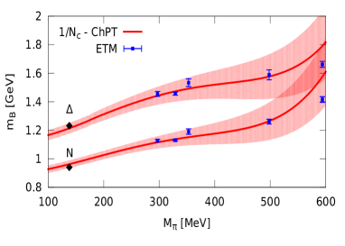
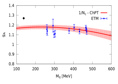
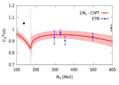
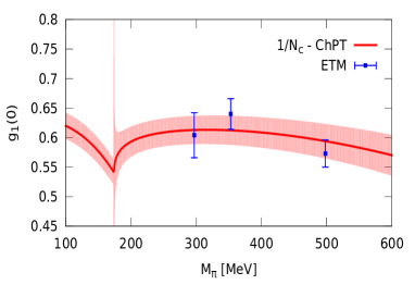
Figure 2: Combined at NNLO to the masses and axial coupling of the ETM collaboration [14, 15, 16]. The diamonds depict the physical values. The bands correspond to the theoretical 68% confidence interval.

The combined fit to the $N$ and $\Delta$ masses at ${\cal{O}}(\xi^{3})$ and the axial couplings at ${\cal{O}}(\xi^{2})$ as functions of $M_{\pi}$ are carried out for the available data below $M_{\pi}\sim 500$ MeV. The results obtained are displayed in Table 1 and in Fig. 2. The $\Delta$ width is used to determine the physical value of $C_{5}^{A}$ according to: $\Gamma_{\Delta\to N\pi}=\frac{C_{5}^{A^{2}}}{6\pi F_{\pi}^{2}}((m_{N}-m_{\Delta})^{2}-M_{\pi}^{2})^{3/2}$, which upon using $\Gamma_{\Delta\to N\pi}^{\rm Exp}=116-120$ MeV, gives $C_{5}^{A}\sim 1.05\pm 0.01$. As emphasized in [1] this corresponds vis-à-vis the nucleon axial coupling to a remarkably small deviation from the $SU(4)$ symmetry limit. One can see that the LQCD results show, for the $\Delta N$ axial coupling, a similar deficit when extrapolated to the physical point as it occurs for the $N$ axial coupling. The cusp observed in the axial couplings involving the $\Delta$ are due to the opening of the $\Delta\to N\pi$ channel. Its location is not the physical one because the baryon masses in the loop are the ones at ${\cal{O}}(\xi)$.

The rather flat behavior of the lattice results for the axial couplings within the mass range considered here is reasonably reproduced by the effective theory; the LECs turn out to have natural size. There is however some curvature in the effective theory, resulting mostly from the non-analytic contributions, which will require more accurate LQCD results to be tested. As it was discussed in Ref. [1] at length, the small dependence with $M_{\pi}$ can only be reproduced thanks to the cancellations dictated by the spin-flavor symmetry between different one-loop contributions. The LECs $C_{2}^{A}$, $C_{3}^{A}$ give spin-flavor breaking contributions to the axial couplings. Their natural size is 1, but they are significantly smaller as a result of the fit, which gives indication of the spin-flavor breaking in the axial couplings to be suppressed dynamically, as it was mentioned earlier.

As it is known from all LQCD extrapolations to the physical pion mass, $g_{A}^{NN}$ is underestimated by about 10%, and a similar underestimation occurs with $C_{5}^{A}$. This is an open issue which in Ref. [1] is argued to be of some systematic LQCD origin, and which should be clarified in forthcoming LQCD calculations.

4 Conclusions

The $1/N_{c}$ expansion at the hadronic level has many claims to fame. It provides an additional bookkeeping tool which is rigorously rooted in QCD, and its blending with effective theories, in particular ChPT, represents the ultimate paradigm for the description of the strong interactions at the hadronic level. It is particularly important in baryons, where the improvement over ordinary BChPT including only the spin-1/2 baryon degrees of freedom is evident. The applications to masses and axial couplings have been worked out [1, 17, 18], and confronted with LQCD results as discussed here. Further applications are very promising, so stay tuned.

The authors thank C. Alexandrou for useful communications regarding the ETM results.

References

- [1] A. C. Cordón and J. L. Goity, Phys. Rev. D 87, 016019 (2013).
- [2] J. -L. Gervais and B. Sakita, Phys. Rev. Lett. 52, 87 (1984).
- [3] R. F. Dashen and A. V. Manohar, Phys. Lett. B 315, 425 (1993).
- [4] E. E. Jenkins, Phys. Rev. D 53, 2625 (1996).
- [5] E. Witten, Nucl. Phys. B 160, 57 (1979).
- [6] R. Flores-Mendieta, C. P. Hofmann, E. E. Jenkins and A. V. Manohar, Phys. Rev. D 62, 034001 (2000).
-
[7]
A. Walker-Loud, these proceedings.
D. Renner, these proceedings. - [8] T. DeGrand, Phys. Rev. D 86, 034508 (2012),
- [9] S. L. Adler, Annals Phys. 50, 189 (1968).
- [10] S. L. Adler, Phys. Rev. D 12, 2644 (1975).
- [11] C. H. Llewellyn Smith, Phys. Rept. 3, 261 (1972).
- [12] J. Beringer et al. [Particle Data Group Collaboration], Phys. Rev. D 86, 010001 (2012).
- [13] R. F. Dashen, E. E. Jenkins and A. V. Manohar, Phys. Rev. D 51, 3697 (1995).
- [14] C. Alexandrou et al. [ETM Collaboration], Phys. Rev. D 83, 045010 (2011),
- [15] C. Alexandrou et al., Phys. Rev. Lett. 107, 141601 (2011),
- [16] C. Alexandrou, private communication.
- [17] R. Flores-Mendieta and C. P. Hofmann, Phys. Rev. D 74, 094001 (2006).
- [18] R. Flores-Mendieta, M. A. Hernandez-Ruiz and C. P. Hofmann, Phys. Rev. D 86, 094041 (2012),