The Redshift Distribution of Intervening Weak Mgii Quasar Absorbers and a Curious Dependence on Quasar Luminosity

Abstract

We have identified 469 Mgii $\lambda\lambda 2796,2803$ doublet systems having $W_{r}\geq 0.02$ Å in 252 Keck/HIRES and UVES/VLT quasar spectra over the redshift range $0.1<z<2.6$. Using the largest sample yet of 188 weak Mgii systems ($0.02$ Å $\leq W_{r}<0.3$ Å), we calculate their absorber redshift path density, $dN/dz$. We find clear evidence of evolution, with $dN/dz$ peaking at $z\sim 1.2$, and that the product of the absorber number density and cross section decreases linearly with increasing redshift; weak Mgii absorbers seem to vanish above $z\simeq 2.7$. If the absorbers are ionized by the UV background, we estimate number densities of $10^{6}-10^{9}$ per Mpc³ for spherical geometries and $10^{2}-10^{5}$ per Mpc³ for more sheetlike geometries. We also find that $dN/dz$ toward intrinsically faint versus bright quasars differs significantly for weak and strong ($W_{r}\geq 1.0$ Å) absorbers. For weak absorption, $dN/dz$ toward bright quasars is $\sim 25\%$ higher than toward faint quasars (10 $\sigma$ at low redshift, $0.4\leq z\leq 1.4$, and 4 $\sigma$ at high redshift, $1.4<z\leq 2.34$). For strong absorption the trend reverses, with $dN/dz$ toward faint quasars being $\sim 20\%$ higher than toward bright quasars (also 10 $\sigma$ at low redshift and 4 $\sigma$ at high redshift). We explore scenarios in which beam size is proportional to quasar luminosity and varies with absorber and quasar redshifts. These do not explain $dN/dz$’s dependence on quasar luminosity.

1. Introduction

Quasar absorption line systems are an extremely useful means of statistically constraining the various scenarios of metal enrichment, inflow and outflow, ionization conditions, kinematics, and gas structure within galaxies and the IGM. Various Mgii absorption line studies have concluded that these systems are cosmologically distributed (Lanzetta et al., 1987; Sargent et al., 1988; Steidel & Sargent, 1992), and numerous subsequent studies have identified specific galaxies associated with Mgii absorption (see Bergeron & Boissè, 1991; Steidel, Dickinson, & Persson, 1994; Steidel et al., 1997; Guillemin & Bergeron, 1997; Churchill et al., 2005; Chen & Tinker, 2008; Kacprzak et al., 2008; Barton & Cooke, 2009; Chen et al., 2010; Kacprzak et al., 2011; Churchill et al., 2012; Nielsen et al., 2012).

For the following discussion, we adopt the terms “weak”, “intermediate”, and “strong” to refer to absorbers having $0.02$ Å $\leq W_{r}<0.3$ Å, $0.3$ Å $\leq W_{r}<1.0$ Å, and $W_{r}\geq 1.0$ Å, respectively, where $W_{r}$ is the rest frame equivalent width of the Mgii $\lambda$2796 transition. Mgii-selected gas probes a wide range of Hi column density environments. Weak Mgii absorption in particular, which samples optically thin gas over a large span of cosmic time, has been proposed to sample dwarf or LSB galaxies as well as the IGM (Churchill et al., 1999; Rigby et al., 2002). However, there are instances in which weak Mgii is identified in the circumgalactic medium of “normal” bright galaxies (Churchill et al., 2012). Milutinović et al. (2006), using an ionization model, concluded that filamentary and sheetlike IGM structures host at least a portion of weak Mgii absorption. Moreover, Nielsen et al. (2012) argue that $W_{r}<0.1$ Å absorbers likely reside in the IGM. Photoionization modeling of weak Mgii systems with associated Civ led Lynch & Charlton (2007) to argue for a scenario of a shell geometry as might be expected for supernova remnants or high velocity clouds moving in a hot corona.

Better insight into the nature of the structures selected by weak Mgii absorbers remains elusive and partially motivates this study. Measurements of the redshift path density $dN/dz$ of weak Mgii absorbers place important constraints on $n(z)\sigma(z)$, the product of their number density and cross section (Churchill et al., 1999; Rigby et al., 2002; Narayanan et al., 2007). In the same vein, probing discrepancies in redshift path densities of Mgii absorption in various equivalent width ranges based on differences in the background sources may reveal information about these absorbing structures. Despite the evidence indicating that absorption line systems are primarily associated with intervening gas as opposed to the background source itself, several studies have nevertheless revealed major discrepancies, depending on the nature of the background source, in the incidence of these absorbers per unit redshift.

Stocke & Rector (1997), in a study of strong Mgii absorbers in BL Lac objects, observed a redshift path density of 4–5 times greater than that expected from quasar surveys. Prochter et al. (2006b) compared quasar and GRB sightlines and found the latter to have a factor of $\sim 4$ excess in the redshift path density of strong absorbers. A similar study by Vergani et al. (2009) found a factor of $\sim 2$ excess of strong absorbers, but no excess of intermediate absorbers, in the GRB sample. Bergeron et al. (2011) reported a factor of $\sim 2$ excess of both strong and intermediate absorbers in blazar versus quasar sightlines. It should be noted, however, that in that study the authors did find marginal statistical evidence in the strong sample of an excess occurring nearer the blazar (even after excluding absorbers having velocity separations of less than 5,000 km s^-1 from the emission redshift). Finally, in a study analyzing Mgii absorbers down to $W_{r}=0.07$ Å in GRB sightlines, Tejos et al. (2009) found a factor of $\sim 3$ overabundance of strong absorbers and a $\sim 30\%$ reduction for $0.07\leq W_{r}<1.0$ Å compared to studies of quasar sightlines. The latter discrepancy, however, was deemed insignificant since the results were consistent at the $1~{}\sigma$ confidence level. Tejos et al. (2009) have so far presented the only study to compare redshift path density differences in weak Mgii absorbers based on different types of background sources.

In this paper we present the largest study of weak Mgii absorption to date, and for the first time provide a parameterized fit to the redshift path density evolution. We also present our findings of differential absorber redshift path density, based on the absolute magnitude of the background quasar, for weak, intermediate, and strong Mgii systems. In § 2 we present our data, and in § 3 our results. We discuss plausible interpretations in § 4, and conclude in § 5. The cosmological parameters $H_{0}=70$ km s^-1 Mpc^-1, $\Omega_{m}=0.3$, and $\Omega_{\Lambda}=0.7$ are adopted throughout.

2. Data and Subsamples

We have searched 252 Keck/HIRES and UVES/VLT quasar spectra for Mgii $\lambda\lambda 2796,2803$ doublet absorption. All systems were objectively identified using the methods of Schneider et al. (1993) and Churchill et al. (1999). Further details are provided in Evans (2011) and Evans, Churchill & Murphy (2012). The search space omitted redshifts within 5,000 km s^-1 of the quasar emission redshift, $z_{em}$, and blueward of the Ly$\alpha$ emission of the quasar. A total of 422 absorbers comprise our sample.

We divided the absorbers into three subsamples using historically motivated weak (Churchill et al., 1999), intermediate (Steidel & Sargent, 1992; Nestor et al., 2005), and strong (Steidel & Sargent, 1992; Nestor et al., 2005) equivalent width ranges. In order to determine whether our absorber subsamples are consistent with being cosmologically distributed along the lines of sight to the quasars, we performed the second test of Bahcall & Peebles (1969). Performing the Kolmogorov-Smirnov (KS) test for each of our equivalent width ranges, we could not rule out that their distributions are consistent with being cosmological. This result is in agreement with earlier studies (Lanzetta et al., 1987; Sargent et al., 1988; Steidel & Sargent, 1992).

Since none of the quasars in our sample were observed with a priori knowledge of weak absorption, our survey is unbiased for this population. However, since the quasar sample is drawn from a broad range of targeted science programs, there is the possibility of bias in the intermediate and strong absorbers, which are known to sometimes be associated with DLAs (Rao & Turnshek, 2000), or which in some cases were already known due to previous lower resolution surveys.

To examine whether our intermediate and strong absorber samples are consistent with an unbiased population, we compared our measured equivalent width distributions, $f(W_{r},W_{\ast})$, where $W_{\ast}$ is the characteristic $W_{r}$, to the distribution measured by Nestor et al. (2005). Using the KS test for the three redshift bins measured by Nestor et al. (2005), we obtained $P({\rm KS})=0.053$ ($0.36\leq z\leq 0.87$), $0.621$ ($0.87\leq z\leq 1.31$) and $0.322$ ($1.31\leq z\leq 2.27$), respectively. For the full redshift range encompassing all three bins, we obtained $P({\rm KS})=0.115$. Even in the case of the lowest value of $P({\rm KS})$, corresponding to the lowest redshift range, the two populations are not inconsistent with each other to even a $2~{}\sigma$ level. We thus proceed under the assumption that our sample of absorbers is a fair sample.

For our analysis in § 3, we obtained absolute $B$-band and apparent magnitudes (primarily $B$, $V$, and $R$) of the quasars. The majority were obtained from Veron-Cetty & Veron (2001); 16 were obtained from the NASA/IPAC Extragalactic Database; and for two quasars, the magnitudes could not be determined so these lines of sight and their absorbers were omitted from analysis for which these quantities were required.

3. Results

Following the formalism of Lanzetta et al. (1987), modified to account for the doublet ratio (Churchill et al., 1999), we calculated the number of absorbers per unit redshift, $dN/dz$.

3.1. Weak Absorber Redshift Path Density

For our full redshift range, $0.1\leq z_{abs}\leq 2.6$, the cumulative redshift path is $\Delta Z=231$ and is $\sim 100$% complete to a 5 $\sigma$ equivalent width sensitivity of $W_{r}(2796)=0.05$ Å and $\sim 82$% complete to a 5 $\sigma$ equivalent width sensitivity of $W_{r}(2796)=0.02$ Å. Over the redshift range $0.4\leq z_{abs}\leq 2.4$, the extent of a study by Narayanan et al. (2007), we have $\Delta Z=213$, compared to their 70; and for $0.4\leq z_{abs}\leq 1.4$, the extent of a study by Churchill et al. (1999), we have $\Delta Z=148$, compared to their 17. These represent the largest two previous weak Mgii surveys. Our larger cumulative redshift path reflects the larger number of lines of sight included in our survey. Churchill et al. (1999) surveyed 26 HIRES quasar spectra and found 30 weak systems, while Narayanan et al. (2007) surveyed 81 UVES quasar spectra and found 112 weak systems. In our survey we identified 188 weak systems.

We calculated $dN/dz$ for weak systems in four redshift bins in order to facilitate comparison with the works of Narayanan et al. (2007) and Churchill et al. (1999); the bins and results are shown in Table 1.

Table 1$dN/dz$  for Mgii Surveys of $0.02$ Å $\leq W_{r}<0.3$ Å

Survey	$0.4\!<\!z\!<\!0.7$	$0.7\!<\!z\!<\!1.0$	$1.0\!<\!z\!<\!1.4$	$1.4\!<\!z\!<\!2.4$
CRCV99	$1.43\pm 0.21$	$1.84\pm 0.26$	$2.19\pm 0.80$	$\cdots$
NMCK07	$1.06\pm 0.10$	$1.51\pm 0.09$	$1.76\pm 0.08$	$1.06\pm 0.04$
this survey	$0.74\pm 0.02$	$1.08\pm 0.02$	$0.95\pm 0.02$	$0.67\pm 0.01$

All three studies obtained different results, with the trend being that the $dN/dz$ values have decreased with larger survey size. All three used the identical code (SEARCH, Churchill et al., 1999) for line and candidate identification, and all three ostensibly used the same algorithms in determining the redshift paths for each system. To test for possible differences in the calculations, we ran our code used for this survey on the identical spectra and set of systems used by Churchill et al. (1999) and compared their $\Delta Z$ and $dN/dz$ results with those of the reproduced study. The result was that the $\Delta Z$ values from the Churchill et al. (1999) study were $\sim 30\%$ larger than our reproduced values from their data, and the $dN/dz$ values from the original study were thereby lowered compared to our reproduced study. This suggests that our redshift path calculations are more conservative than those of Churchill et al. (1999). If our redshift paths had been calculated exactly as theirs, the $dN/dz$ result of this survey would presumably have been lower, further widening the discrepancy with previous works. A similar duplication of the survey of Narayanan et al. (2007) could not be performed because a significant number of the authors’ quasar spectra were unavailable to us.

In an attempt to find differences in the quasar samples that could possibly lead to the discrepant $dN/dz$ results among the three works, we investigated the quasar apparent magnitude distributions. The KS test was performed between all possible pairs of the three surveys. Our survey and that of Narayanan et al. (2007) exhibit remarkably similar distributions; it could not be ruled out to greater than a $1\sigma$ confidence level that their apparent magnitudes had been drawn from the same population, and their median values were both 17.5. In contrast, the Churchill et al. (1999) survey differed from each of the other two to a confidence level of $4\sigma$ and had a median apparent magnitude of 16.3. A uniform set of apparent magnitudes in the same band was not available, however, making these comparisons uncertain. The smaller Churchill et al. (1999) survey was undoubtedly overall biased toward brighter quasars.

We likewise investigated the quasar absolute $B$-band magnitude distributions, but when each survey was tested against the other two, it could not be ruled out to even a $1\sigma$ confidence level that their distributions had been drawn from the same population. Similarly, no substantial differences were found in the overall median quasar absolute magnitude of the three surveys: $-28.5$, $-28.7$, and $-28.6$ for Churchill et al. (1999), Narayanan et al. (2007), and this study, respectively.

The reasons behind the different $dN/dz$ results among the three works remain unclear; future studies will hopefully resolve the weak Mgii puzzle. It may be that the inclusion or exclusion of weak systems very close to the limiting equivalent width may play a role (Anand Narayanan, private communication), as well as differences in the codes used, since the calculation of $\Delta Z$ is extremely sensitive for the weakest systems.

3.2. Redshift Evolution

The number of absorbers per unit redshift is the product of the proper number density of absorbers and their proper geometric cross section. In the standard cosmological model, the no-evolution expectation (NEE) for the redshift number density can be parameterized as:

$$\left[{dN\over dz}\right]_{\hbox{\tiny NEE}}={c\over H_{0}}n_{0}\sigma_{0}{(1+z)^{2}\over\sqrt{\Omega_{m}(1+z)^{3}+\Omega_{\Lambda}}}$$ (1)

where $n_{0}$ is the mean comoving number density of absorbers and $\sigma_{0}$ is the mean comoving geometric absorber cross section. As shown in Figure 1$a$, our observed $dN/dz$ departs strikingly from the NEE (dashed curve), which was normalized to the mean $z_{abs}$, 1.098, and to the overall $dN/dz$, 0.83, of our weak sample over the redshift range $0.1\leq z_{abs}\leq 2.6$. The general behavior of $dN/dz$ is in agreement with Narayanan et al. (2007) in that it peaks between $1.0<z<1.4$ and then decreases toward higher redshift.

If the product $n\sigma$ varies as a function of redshift, $dN/dz$ may depart from the no-evolution expectation. The quantity $n(z)\sigma(z)$ can be written as

$$n(z)\sigma(z)=n_{0}\sigma_{0}f(z),$$ (2)

where $f(z)$ is a nonnegative function that parameterizes the evolution of $dN/dz$.

Figure 1$b$ depicts our weak $dN/dz$ result divided by the NEE. The data clearly motivate a linear fit; this was achieved using a function of the form

$$f(z)=1-\alpha(z-z^{*}),$$ (3)

where $\alpha$ is the slope and $z^{*}$ is the function normalization. The result, $\alpha=0.69\pm 0.02$ and $z^{*}=1.29\pm 0.05$, is shown as a solid line in Figure 1$b$.

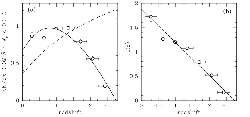
Figure 1.— ($a$) shows the weak $dN/dz$ (open circles) as well as the NEE (dashed line). — ($b$) shows the same data divided by the NEE. The solid line is the best linear fit to this ratio. In ($a$), this fit was then multiplied by the NEE and plotted (solid curve).

Finally, the fit to $f(z)$ was multiplied by the NEE, yielding a fit to the $dN/dz$ result in Figure 1$a$ (solid curve) that can be expressed as

$${dN\over dz}={c\over H_{0}}n_{0}\sigma_{0}{(1+z)^{2}\left[1-\alpha(z-z^{*})\right]\over\sqrt{\Omega_{m}(1+z)^{3}+\Omega_{\Lambda}}}\qquad(z<2.74)\,.$$ (4)

Weak Mgii absorbers seem to vanish at high redshift; this result is discussed in § 4.

3.3. Differential Absorber Redshift Path Densities by Absolute Magnitude

Motivated by studies that found differences in $dN/dz$ results based on background object as discussed in § 1, as well as our finding of differing apparent magnitude distributions among the weak Mgii studies as discussed in § 3.1, we attempted to discern some intrinsic difference that might affect the observed $dN/dz$. Using the absolute $B$-band quasar magnitudes of our survey, which had a range of $-32.2\leq M_{B}\leq-19.8$, we divided our quasars into “bright” and “faint” subsamples according to the median, $\left<M_{B}\right>=-28.6$. The bright subsample has a median of $-29.4$, and the faint subsample has a median of $-27.4$.

Table 2$dN/dz$ by Quasar Luminosity

sample	weak	sig	intermediate	sig	strong	sig
	$0.02\leq W_{r}<0.3$	lev	$0.3\leq W_{r}<1.0$	lev	$W_{r}\geq 1.0$	lev
$0.4\leq z_{abs}\leq 1.4$
all	$0.931\pm 0.006$		$0.715\pm 0.005$		$0.449\pm 0.003$
bright	$1.040\pm 0.016$		$0.692\pm 0.010$		$0.406\pm 0.006$
faint	$0.836\pm 0.011$		$0.730\pm 0.009$		$0.481\pm 0.006$
bright/all	$1.117\pm 0.019$	$6.2~{}\sigma$	$0.967\pm 0.016$	$2.1~{}\sigma$	$0.905\pm 0.015$	$6.3~{}\sigma$
faint/all	$0.897\pm 0.013$	$7.9~{}\sigma$	$1.021\pm 0.014$	$1.5~{}\sigma$	$1.072\pm 0.015$	$4.8~{}\sigma$
faint/bright	$0.803\pm 0.020$	$9.9~{}\sigma$	$1.056\pm 0.019$	$2.9~{}\sigma$	$1.185\pm 0.019$	$9.7~{}\sigma$
$1.4<z_{abs}\leq 2.34$
all	$0.686\pm 0.011$		$0.696\pm 0.011$		$0.631\pm 0.010$
bright	$0.732\pm 0.018$		$0.730\pm 0.018$		$0.584\pm 0.014$
faint	$0.579\pm 0.028$		$0.619\pm 0.030$		$0.714\pm 0.034$
bright/all	$1.068\pm 0.031$	$2.2~{}\sigma$	$1.050\pm 0.031$	$1.6~{}\sigma$	$0.926\pm 0.027$	$2.7~{}\sigma$
faint/all	$0.845\pm 0.043$	$3.6~{}\sigma$	$0.890\pm 0.045$	$2.4~{}\sigma$	$1.131\pm 0.057$	$2.3~{}\sigma$
faint/bright	$0.791\pm 0.054$	$3.9~{}\sigma$	$0.848\pm 0.054$	$2.8~{}\sigma$	$1.222\pm 0.053$	$4.1~{}\sigma$

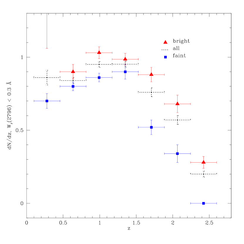
Figure 2.— $dN/dz$ of the weak sample for the bright (red triangles), faint (blue squares), and combined (dotted crosses) samples. In the bright sample, the lowest redshift data point has a value of $1.53\pm 0.47$.

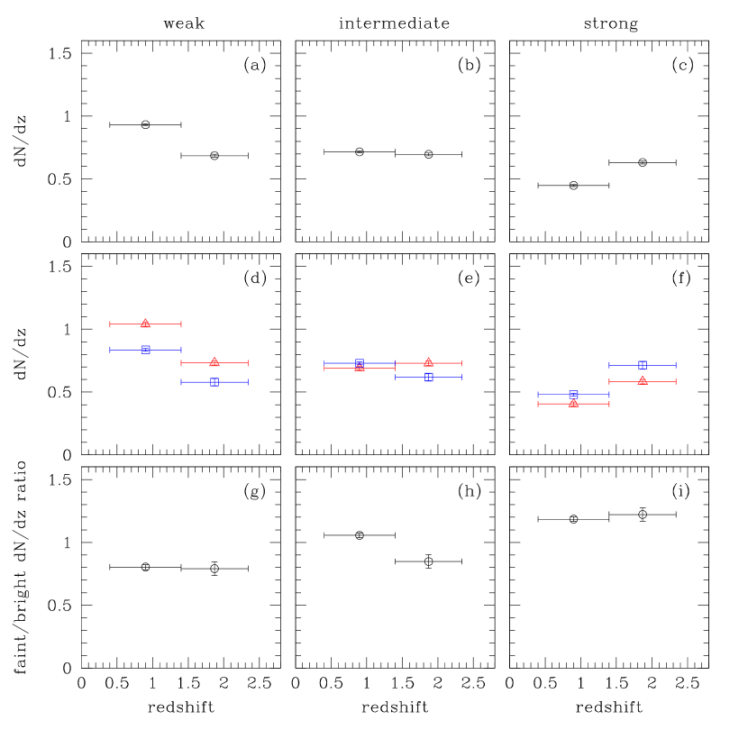
Figure 3.— ($a$–$c$) show $dN/dz$ of the weak, intermediate and strong samples, respectively, in two redshift bins ($0.4\leq z_{abs}\leq 1.4$ and $1.4\leq z_{abs}\leq 2.34$). — ($d$–$f$) show $dN/dz$ for the bright (red triangles) and faint (blue squares) subsamples. The points were left open to better display the error bars. — ($g$–$i$) show the faint to bright $dN/dz$ ratio.

Figure 2 shows our weak $dN/dz$ results for the bright and faint samples binned as in Figure 1. The redshift path density of the bright sample is clearly higher than that of the faint sample at all redshifts. The lowest redshift bin of the weak bright sample contained only five systems and we believe this caused the $dN/dz$ result in that bin to be less reliable.

Figures 3$a$–3$c$ plot our $dN/dz$ results for weak, intermediate and strong Mgii absorption. The bins ($0.4\leq z_{abs}\leq 1.4$ and $1.4\leq z_{abs}\leq 2.34$, “low” and “high” redshift) were selected based on previous studies (Narayanan et al., 2007; Nestor et al., 2005; Churchill et al., 1999). Similarly, Figures 3$d$–3$f$ show $dN/dz$ calculated for the faint and bright quasar samples. Figures 3$g$–3$i$ show the ratio of the $dN/dz$ results of the faint quasar sample to that of the bright. These values are listed in Table 2 for each $W_{r}$ and redshift range. Though the weak $dN/dz$ results of Churchill et al. (1999), Narayanan et al. (2007), and this study all differed as discussed in § 3.1, the relative values among our own faint, bright and all quasar subsamples are robust, having been calculated in a consistent manner. Similarly, though our intermediate and strong samples have $W_{r}$ distributions consistent with Nestor et al. (2005) as mentioned in § 2, our $dN/dz$ results for these samples are higher than those of Nestor et al. (2005) and Lundgren et al. (2009). This is expected since some of the quasars in our survey were targeted for their known $W_{r}\geq 0.3$ Å Mgii absorption; however, the $dN/dz$ ratios between our magnitude bins are robust.

For weak systems, the $dN/dz$ values toward bright quasars are $\sim 25\%$ higher than for the faint in both redshift ranges, while for strong systems, $dN/dz$ is $\sim 20\%$ higher toward faint quasars than toward bright in both redshift ranges. The faint to bright $dN/dz$ ratio, $(dN/dz)_{f}/(dN/dz)_{b}$, departs for the weak systems from unity at the $\simeq 10~{}\sigma$ level for low redshift and at the $\simeq 4~{}\sigma$ level for high redshift. The strong absorber ratios are similarly significant (see Table 2), though in that case the faint quasar $dN/dz$ values are higher, rather than lower, than those of the bright sample. In the case of the intermediate absorbers the ratio is consistent with unity within $3~{}\sigma$.

In the calculation of $dN/dz$ the sensitivity of each spectrum is accounted for (see Lanzetta et al., 1987; Evans, 2011), eliminating the possibility that the higher values of the weak bright sample compared to the weak faint sample might result from higher signal-to-noise ratios.

4. Discussion

Based on our weak $dN/dz$ result (see Figure 1), the cosmic number density, geometric cross section, or both, of weak Mgii absorbers appear to be evolving. The apparent dropoff in our fit toward $z=0$ may be overly steep; it is possible that the weak $dN/dz$ peaks at $z\sim 1$, declines slightly and then levels off toward the present. However, it is a first attempt to characterize weak Mgii absorber evolution using a functional form. Our result predicts that no such absorbers exist above $z\simeq 2.7$.

Narayanan et al. (2007) speculated that the apparent paucity of weak Mgii above $z\sim 2$ might be due to the high redshift analogs of low redshift weak Mgii absorption being associated with strong Mgii. In this scenario, weak Mgii absorption at high redshift would be in the kinematic vicinity of strong Mgii and thus would not be recognized as isolated weak absorption. However, we have compared the high velocity weak kinematic subsystems of strong Mgii subsystems to isolated weak Mgii absorption (Evans, 2011). Morphologically these two types of profiles often appear very similar, but a KS test of their rest equivalent width distributions revealed that they are actually two distinct populations to a 99.98% confidence level, or greater than 3 $\sigma$. A KS test of the distributions of flux decrement-weighted velocity spreads, $\omega_{v}$ (Churchill & Vogt, 2001; Evans, 2011) indicated to a greater than 6 $\sigma$ confidence level that the two populations are unique.

The $dN/dz$ evolution we detect in weak Mgii may be due to changes in gas structure or ionization conditions; neither we nor other studies find the same falloff in intermediate and strong Mgii absorption (Nestor et al., 2005; Prochter et al., 2006a; Lundgren et al., 2009) up to our maximum redshift of $2.6$. Matejek & Simcoe (2012) do report a decline in the strong population above $z\sim 3$, and note that this peak corresponds to that of the SFR. Our weak $dN/dz$ result, which exhibits no such peak, may provide indirect evidence that a substantial fraction of these absorbers resides in the IGM, since their evolution appears not to correspond to star formation.

Using Cloudy 08.00 photoionization modeling (Ferland et al., 1998), we investigated the evolution of weak Mgii absorber sizes $R(z)$ and cosmic number densities $n(z)$ (for additional details see Evans, 2011). In this scenario Mgii selects relatively dense cloudlets embedded within plane parallel slabs of gas. We modeled optically thin clouds having a range of hydrogen number densities based on past Mgii photoionization modeling results (Rigby et al., 2002; Bergeron et al., 2002). We assumed an ultraviolet background model that varies as a function of $z$, following the work of Haardt & Madau (1996), which includes the contribution of galaxies. Though we examined a grid of clouds with a range of Hi column densities and metallicities, we discuss here clouds having $N(\hbox{{\rm H}\kern 1.00006pt{\sc i}})$ of $10^{16}$ cm^-2 and a metallicity of 0.1 solar. For weak Mgii, $\log N({\hbox{{\rm H}\kern 1.00006pt{\sc i}}})$ is constrained to the range 15.5–17.0 cm^-2 (Churchill et al., 2000; Rigby et al., 2002).

The resulting cloud thicknesses, which we interpreted as absorber sizes $R(z)$ and which are governed by the ionizing background, peak at $z\sim 2$ and then decline toward the present, as shown in Figure 4$a$. Assuming spherical clouds, the corresponding absorber cross sections $\sigma(z)$, combined with our weak $dN/dz$ constraint using the fit of Equation 4, translate into cosmic absorber number densities $n(z)$ that increase monotonically toward the present (Figure 4$b$). The absorber sizes produced by this model are on the order of a parsec, and yield absorber number densities on the order of $10^{6}-10^{9}$ Mpc^-3, for the middle range of $n_{H}$ values. This corresponds to $10^{9}$–$10^{12}$ absorbers per $L^{*}$ galaxy for $z\lesssim 1$ (Faber et al., 2007) as well as for $1\lesssim z\lesssim 3$ (Reddy & Steidel, 2009; Oesch et al., 2010).

If the clouds are not spherical, but instead the transverse extent $R_{T}$ scales with cloud thickness according to a factor $\beta$ such that $R_{T}=\beta R(z)$, then $n(z)$ would scale as $\beta^{-2}$. For $\beta=100$, $n(z)$ would then be reduced by a factor of $10^{4}$, which yields $10^{2}-10^{5}$ weak absorbers per Mpc³. It should be noted that changing the model’s $N({\hbox{{\rm H}\kern 1.00006pt{\sc i}}})$ would change $R(z)$ in direct proportion, while $n(z)$, using our $dN/dz$ constraints, would vary as $N({\hbox{{\rm H}\kern 1.00006pt{\sc i}}})^{-2}$.

Figure 4.— ($a$) plots the evolution of Cloudy absorber size, log $R(z)$. ($b$) plots the number density of absorbers, log $n(z)$. The dashed curves represent log $n_{H}=-0.5$ cm^-3; the dotted curves, log $n_{H}=-1.0$ cm^-3; the solid curves, log $n_{H}=-1.5$ cm^-3; the long dashed curves, log $n_{H}=-2.0$ cm^-3; and the dashed-dotted curves, log $n_{H}=-2.5$ cm^-3.

Our Cloudy model is suggestive of a condensation mechanism into sheet or filament structures characteristic of the IGM. Sheetlike geometries require far fewer weak absorbers than do spherical geometries per $L^{*}$ galaxy, and therefore we consider these to be a more realistic scenario. Although we do not fully explain the nature of weak Mgii absorption, this exercise does provide a limiting case in which to couch the phenomenon. Our absorber size estimate is not far from that of Rigby et al. (2002), who concluded that a sheetlike structure containing many embedded $\sim 10$ pc absorbers was required to account for the observed $dN/dz$. Recent findings by Churchill et al. (2012) and Nielsen et al. (2012) indicate that $0.1\leq W_{r}\leq 0.3$ Å, but not $0.02\leq W_{r}\leq 0.1$ Å, absorbers are found in the circumgalactic medium of normal galaxies at impact parameters of less than 200 kpc. They suggest that the weaker of these two populations may then reside primarily in the IGM.

Our $dN/dz$ results toward faint versus bright absolute magnitude quasars reveal that the weak absorbers have a higher redshift path density in the bright quasar sample than in the faint at both low and high redshifts. For the strong absorbers, the opposite is true. The intermediate absorbers appear to follow no clear trend, and may represent an equivalent width range where the effects leading to the weak and strong differentials mostly cancel.

Following the discovery by Prochter et al. (2006b) of the quasar–GRB strong Mgii discrepancy, various researchers have attempted to explain the phenomenon. Frank et al. (2007) modeled the effects of Mgii absorber size and impact parameter on observed equivalent width and concluded that the $dN/dz$ discrepancy may be due to the larger beam sizes of quasars versus GRBs, the latter of which they state are on the order of the sizes of cloud cores. The authors also predicted that different luminosity populations of quasars should contain different incidences and strengths of intervening absorbers.

Porciani et al. (2007) countered this differential beam size argument, noting that no unsaturated Mgii doublets have been observed having a doublet ratio of one, as would be expected in the case of partial covering of a quasar beam by an absorber. They stated that magnification bias could explain the discrepancy, and that dust obscuration bias and association of absorbers with the circumburst environment could also partially account for it.

A statistical study was also conducted by Pontzen et al. (2007) to look for systematically lowered Mgii equivalent widths over quasar broad line emission regions, which are substantially larger than quasar continuum regions; no significant difference was found.

Cucchiara et al. (2009) cite an intrinsic origin as a possible explanation for the GRB excess. Mgii absorbing gas could be ejected at relativistic velocities and masquerade as an intervening absorber; however, the authors note that the presence of Mgi absorption in these systems, as well as the lack of fine structure transitions that are expected in the vicinity of a GRB, cast doubt on this theory. Vergani et al. (2009) concur that the excess could be intrinsic, and estimate required ejection velocities of $10,000-25,000$ km s^-1. They also consider gravitational lensing to be a viable mechanism to account for the discrepancy.

In two studies of Civ absorbers toward GRBs, Sudilovsky et al. (2007) and Tejos et al. (2007) reported no excess incidence over quasar sightlines. Sudilovsky et al. (2007) speculated that the difference in the cases of Mgii versus Civ absorbers arose partially because the former introduced more dust extinction than the latter. However, dust extinction in Mgii absorbers was subsequently modeled (Sudilovsky et al., 2009), and the authors concluded that the effect could only account for $\sim 10\%$ of the quasar–GRB discrepancy.

Tejos et al. (2009) rejected an intrinsic origin for excess GRB Mgii absorbers due to the lack of both excess Civ absorption and excess weak and intermediate Mgii absorption, and instead favored gravitational lensing as the relevant mechanism. Wyithe et al. (2011) modeled gravitational lensing in quasar and GRB sightlines and concluded that it was a feasible explanation for the excess, but that further GRB data were necessary to support or refute their findings. They noted that afterglows in which strong Mgii systems are found are brighter than average, implying a greater lensing rate.

Through their modeling of extinction curves toward quasars and GRBs, Budzynski & Hewett (2011) determined that $dN/dz$ toward quasars would be significantly higher if corrected for dust, and that the correction varies with redshift. The discrepancy compared to GRBs arises, the authors state, because their absorber redshift distribution is shifted higher than that of quasars, resulting in less loss of detected absorbers. They calculated that this effect could account for a factor of two excess in the GRB $dN/dz$.

Keeping these previous studies of the quasar–GRB discrepancy in mind, and in an attempt to understand the possibly related phenomenon we have uncovered, we attempted to find some other metric within our faint and bright quasar samples that would shed light on these issues. The redshift path density depends on the integrated equivalent width distribution,

$${dN\over dz}\propto{\displaystyle\int_{W_{min}}^{W_{max}}\!\!\!f(W,W_{*})\,dW}\,.$$ (5)

We therefore compared equivalent width distributions for our faint and bright quasar samples for the various $W_{r}$ ranges as well as for low, high, and all redshifts.

We also studied equivalent width distributions binned by relative beam sizes using $M_{B}$ as a proxy, i.e. assuming that the square of the source radius $R_{s}$ is proportional to the $B$-band luminosity of the quasar. The ratio of the source radius for quasar $i$ relative to the median radius for the full quasar sample can then be written (Shakura & Sunyaev, 1973) as

$$\frac{R_{s,i}}{\left<R_{s}\right>}=10^{-0.2(M_{i}-\left<M_{B}\right>)}.$$ (6)

We then studied the effect of changing beam size with redshift due to cosmology. We calculated the ratio of the relative beam size of quasar $i$ at the redshift of absorber $j$ to the cross section of the source:

$${\sigma_{b}(z_{j})\over\sigma_{s,i}}=\left[\frac{D_{\hbox{\tiny A}}(z_{j})}{D_{\hbox{\tiny A}}(z_{s,i})}\right]^{2}$$ (7)

where $\sigma_{s,i}=\pi R_{s,i}^{2}$, $D_{A}(z_{j})$ is the angular diameter distance at the absorption redshift of system $j$, and $D_{A}(z_{s,i})$ is the angular diameter distance at the source redshift of quasar $i$. Finally, we examined the combined effect of source size and cosmology, by using Equation 6 to scale $\sigma_{b}$.

Using the KS test, none of these equivalent width distributions yielded significant differences (of at least 3 $\sigma$) between the faint and bright quasar samples. Since the $dN/dz$ discrepancy is in this case of a smaller magnitude than in the case of the quasar–GRB phenomenon, it may require a larger data set to discern the reasons behind the observations.

The findings of Budzynski & Hewett (2011) do offer an intriguing possibility by relating absorption redshift distributions to $dN/dz$. Our faint absorber samples do have lower median $z_{abs}$ values than our bright samples across all three equivalent width ranges, probably a result of the correlation whereby intrinsically more luminous quasars tend to be selected at higher redshifts. This result only supports the authors’ dust argument in the case of our weak absorbers, the only sample in which the absorption incidence is significantly higher toward bright quasars than faint. For our weak sample, the median absorption redshift is $0.87$ in the faint subsample and $1.17$ in the bright. KS testing, however, revealed that it could not be ruled out to a greater than 98.32% confidence level that the faint and bright subsamples are drawn from the same underlying $z_{abs}$ distribution.

Though several authors have argued for an intrinsic origin for excess strong Mgii absorption toward GRBs versus quasars, this does not appear to explain the $dN/dz$ discrepancy in the case of our bright and faint quasar populations. Our Bahcall & Peebles (1969) testing revealed absorber distributions consistent with cosmological within all equivalent width and quasar absolute magnitude subsamples, as well as in the aggregate populations. The velocities of Mgii-selected gas ejected from a quasar would have to reach large fractions of the speed of light in order to pass for intervening systems. It therefore seems highly unlikely that significant intrinsic absorption could be present in our sample.

5. Conclusion

We have found in a survey of 252 quasar spectra that the incidence of weak Mgii absorption evolves markedly, that it peaks at $z\sim 1.2$, and that it is fit by a function that is a product of the no-evolution expectation with a linear function. Our linear fit to the ratio of our $dN/dz$ data to the NEE resulted in a slope of $\alpha=0.69\pm 0.02$ and a normalization of $z^{*}=1.29\pm 0.05$ for the function $f(z)=1-\alpha(z-z^{*})$. Our $dN/dz$ result predicts that no weak Mgii absorbers exist above $z\simeq 2.7$.

We find that when our quasar survey is segregated by absolute magnitude, weak Mgii $dN/dz$ is significantly lower in the faint subsample than in the bright, with faint to bright $dN/dz$ ratios of $0.80\pm 0.02$ at low redshift and $0.79\pm 0.05$ at high redshift. In contrast, strong Mgii $dN/dz$ is significantly higher in the faint subsample than in the bright, with faint to bright $dN/dz$ ratios of $1.19\pm 0.02$ at low redshift and $1.22\pm 0.05$ at high redshift. Intermediate equivalent width absorbers exhibited $dN/dz$ ratios consistent with unity within 3 $\sigma$. At this time it is uncertain whether these results stem from some intrinsic property of the quasars, from some difference in the intervening sightlines, or from some combination of these factors.

References

- Bahcall & Peebles (1969) Bahcall, J. N., & Peebles, P. J. E. 1969, ApJ, 156, L7
- Barton & Cooke (2009) Barton, E. J., & Cooke, J. 2009, AJ, 138, 1817
- Bergeron et al. (2002) Bergeron, J., Aracil, B., Petitjean, P., & Pichon, C. 2002, A&A, 419, 811
- Bergeron & Boissè (1991) Bergeron, J., & Boissè, P. 1991, å, 243, 334
- Bergeron et al. (2011) Bergeron, J., Boissé, P., & Ménard, B. 2011, A&A, 525, 51
- Budzynski & Hewett (2011) Budzynski, J. M., & Hewett, P. C. 2011, MNRAS, 416, 1871
- Chen et al. (2010) Chen, H.-W., Helsby, J. E., Gauthier, J.-R., Shectman, S. A., Thompson, I. B., & Tinker, J. L. 2010, ApJ, 714, 1521
- Chen & Tinker (2008) Chen, H.-W., & Tinker, J. L. 2008, ApJ, 687, 745
- Churchill et al. (2012) Churchill, C. W., Kacprzak, G. G., Nielsen, N. M., Steidel, C. C., & Murphy, M. T. 2012, ApJ, submitted
- Churchill et al. (2005) Churchill, C. W., Kacprzak, G. G., & Steidel, C. C. 2005, IAU Colloq. 199: Probing Galaxies through Quasar Absorption Lines, 24
- Churchill et al. (1999) Churchill, C. W., Rigby, J. R., Charlton, J. C., & Vogt, S. S. 1999, ApJS, 120, 51
- Churchill et al. (2000) Churchill, C. W., Mellon, R. R., Charlton, J. C., Jannuzi, B. T., Kirhakos, S., Steidel, C. C., & Schneider, D. P. 2000, ApJS, 130, 91
- Churchill & Vogt (2001) Churchill, C. W., & Vogt, S. S. 2001, ApJ, 122, 679
- Cucchiara et al. (2009) Cucchiara, A., Jones, T., Charlton, J. C., Fox, D. B., Einsig, D., & Narayanan, A. 2009, ApJ, 697, 345
- Evans (2011) Evans, J. L. 2011, Ph.D. thesis, New Mexico State University
- Evans, Churchill & Murphy (2012) Evans, J. L., Churchill, C. W., & Murphy, M. T. 2012, ApJS, in preparation
- Faber et al. (2007) Faber, S. M. et al. 2007, ApJ, 665, 265
- Ferland et al. (1998) Ferland, G. J., Korista, K. T., Verner, D. A., Ferguson, J. W., Kingdon, J. B., & Verner, E. M. 1998, PASP, 110, 761
- Frank et al. (2007) Frank, S., Bentz, M. C., Stanek, K. Z., Mathur, S., Dietrich, M., Peterson, B. M., & Atlee, D. W. 2007, Ap&SS, 312, 325
- Guillemin & Bergeron (1997) Guillemin, P., & Bergeron, J. 1997, å, 328, 499
- Haardt & Madau (1996) Haardt, F., & Madau, P. 1996, ApJ, 461, 20
- Kacprzak et al. (2011) Kacprzak, G. G., Churchill, C. W., Evans, J. L., Murphy, M. T., & Steidel, C. C. 2011, MNRAS, 416, 3118
- Kacprzak et al. (2008) Kacprzak, G. G., Churchill, C. W., Steidel, C. C., & Murphy, M. T. 2008, AJ, 135, 922
- Lanzetta et al. (1987) Lanzetta, K. M., Turnshek, D. A., & Wolfe, A. M. 1987, ApJ, 332, 739
- Lundgren et al. (2009) Lundgren, B. F., Brunner, R. J., York, D. G., Ross, A. J., Quashnock, J. M., Myers, A, D., Schneider, D. P., Al Sayyad, Y., & Bahcall, N. 2009, ApJ, 698, 819
- Lynch & Charlton (2007) Lynch, R. S., & Charlton, J. C. 2007, ApJ, 666, 64
- Matejek & Simcoe (2012) Matejek, M. S., & Simcoe, R. A. 2012, ApJ, submitted
- Milutinović et al. (2006) Milutinović, N., Rigby, J. R., Masiero, J. R., Lynch, R. R., Palma, C., Charlton, J. C. 2006, ApJ, 641, 190
- Narayanan et al. (2007) Narayanan, A., Misawa, T., Charlton, J. C., & Kim, T. 2007, ApJ, 660, 1093
- Nestor et al. (2005) Nestor, D. B., Turnshek, D. A., & Rao, S. M. 2005, ApJ, 628, 637
- Nielsen et al. (2012) Nielsen, N. M., Churchill, C. W., & Kacprzak, G. G. 2012, ApJS, in preparation
- Oesch et al. (2010) Oesch, P. A., Bouwens, R. J., Carollo, C. M., Illingworth, G. D., Magee, D., Trenti, M., Stiavelli, M., Franx, M., Labbé, I., & van Dokkum, P. G. 2010, ApJ, 725, 150
- Pontzen et al. (2007) Pontzen, A., Hewett, P., Carswell, R., & Wild, V. 2007, MNRAS, 381, 99
- Porciani et al. (2007) Porciani, C., Viel, M., & Lilly, S. J. 2007, ApJ, 659, 218
- Prochter et al. (2006a) Prochter, G. E., Prochaska, J. X., & Burles, S. M. 2006a, ApJ, 639, 766
- Prochter et al. (2006b) Prochter, G. E., Prochaska, J. X., Chen, H., Bloom, J. S., Dessauges-Zavadsky, M., Foley, R. J., Lopez, S., Pettini, M., Dupree, A. K., & Guhathakurta, P. 2006b, ApJ, 648, 93
- Rao & Turnshek (2000) Rao, S. M., & Turnshek, D. A. 2000, ApJS, 130, 1
- Reddy & Steidel (2009) Reddy, N.A., & Steidel, C. C. 2009, ApJ, 692, 778
- Rigby et al. (2002) Rigby, J. R., Charlton, J. C., & Churchill, C. W. 2002, ApJ, 565, 743
- Sargent et al. (1988) Sargent, W. L. W., Steidel, C. C., & Boksenberg. A. 1988, ApJ, 334, 22
- Schneider et al. (1993) Schneider, D. P., et al. 1993, ApJS, 87, 45
- Shakura & Sunyaev (1973) Shakura, N. I., & Sunyaev, R. A. 1973, A&A, 24, 337
- Steidel et al. (1997) Steidel, C. C., Dickinson, M., Meyer, D. M., Adelberger, K. L., & Sembach, K. R. 1997, ApJ, 480, 586
- Steidel, Dickinson, & Persson (1994) Steidel, C. C., Dickinson, M., & Persson, S. E. 1994, ApJ, 437, L75
- Steidel & Sargent (1992) Steidel, C. C., & Sargent, W. L. W. 1992, ApJS, 80, 1
- Stocke & Rector (1997) Stocke, J. T., & Rector, T. A. 1997, ApJ, 489, 17
- Sudilovsky et al. (2007) Sudilovsky, V., Savaglio, S., Vreeswijk, P., Ledoux, C., Smette, A., & Greiner, J. 2007, ApJ, 669, 741
- Sudilovsky et al. (2009) Sudilovsky, V., Smith, D., & Savaglio, S. 2009, ApJ, 699, 56
- Tejos et al. (2009) Tejos, N., Lopez, S., Prochaska, J. X., Bloom, J. S., Chen, H., Dessauges-Zavadsky, M., Maureira, M. J. 2009, ApJ, 706, 1309
- Tejos et al. (2007) Tejos, N., Lopez, S., Prochaska, J. X., Chen, H., & Dessauges-Zavadsky, M. 2007, ApJ, 671, 622
- Vergani et al. (2009) Vergani, S. D., Petitjean, P., Ledoux, C., Vreeswijk, P., Smette, A., Meurs, E. J. A. 2009, å, 503, 771
- Veron-Cetty & Veron (2001) Veron-Cetty, M. P., & Veron, P. 2001, A&A, 374, 92
- Wyithe et al. (2011) Wyithe, J. S. B., Oh, S. P, & Pindor, B. 2011, MNRAS, 414, 209