Cosmic Acceleration and Brans-Dicke Theory

Abstract

This paper is devoted to study the accelerated expansion of the universe by exploring the Brans-Dicke parameter in different eras. For this purpose, we take FRW universe model with viscous fluid (without potential) and Bianchi type I universe model with barotropic fluid (with and without potential). We evaluate deceleration parameter as well as Brans-Dicke parameter to explore cosmic acceleration. It is concluded that accelerated expansion of the universe can also be achieved for higher values of the Brans-Dicke parameter in some cases.

Keywords: Brans-Dicke theory; scalar field; cosmic acceleration.
PACs numbers: 04.50.Kd, 98.80.-k;

1 Introduction

The accelerated expansion of the observable universe is one of the most conspicuous and recent achievement in modern cosmology. This expansion with positive cosmic acceleration has been confirmed by many astronomical experiments such as Supernova (Ia) ^1,2), WMAP ³⁾, SDSS ⁴⁾, galactic cluster emission of X-rays ⁵⁾, large scale structure ⁶⁾, weak lensing ⁷⁾ etc. These results lead to the conclusion that our universe is spatially flat.

The positive cosmic acceleration of the universe has been motivated by a mysterious exotic matter having large negative pressure, known as dark energy. Although, General Relativity (GR) is an excellent theory to explain the gravitational effects but it is unable to describe the present cosmic acceleration and the reality of dark energy. In order to explain the nature of this mysterious finding, various models including Chaplygin gas, phantom, quintessence, cosmological constant etc. have been constructed ^8,9). However, none of these models is very successful.

The exploration of scalar-tensor theories of gravity as modified theories of gravity has received much attention due to their vast implications in cosmology ^10-14). Brans-Dicke (BD) theory of gravity, a special case of scalar-tensor theories, is one of the most viable theories for this purpose. It is the general deformation of GR satisfying weak equivalence principle, in which gravity effects are mediated by the metric tensor and the scalar field ¹⁵⁾. This provides a direct coupling of the scalar field to geometry. Brans-Dicke theory is compatible with both Mach’s principle ¹⁶⁾ and Dirac’s large number hypothesis ¹⁷⁾. One of the salient features of this theory is that the gravitational coupling constant, being the inverse of spacetime scalar field, varies with time. In order to fulfill the solar system experiment constraints, the value of the generic dimensionless BD parameter $\omega$ should be very large, i.e., $\omega\geq 40,000$ ^18,19).

Brans-Dicke theory is a successful theory which can tackle many outstanding cosmological problems like inflation, quintessence, late time behavior of the universe, coincidence problem, cosmic acceleration ¹¹⁾ etc. There are different versions of BD theory available in literature ^20,21). Singh and Rai ²²⁾ investigated various BD cosmological models and showed that the Bianchi models are very effective in explaining the evolution of the universe for perfect fluid. Bermann ²³⁾ discussed different models of the universe with constant deceleration parameter based on the variation law of Hubble parameter. Bertolami and Martins ¹¹⁾ found that the accelerated expansion of the universe could be obtained with large $|\omega|$ and potential $\phi^{2}$ without considering the positive energy condition. Sen and Sen ²⁴⁾ showed that the dissipative pressure could support the late time accelerated expansion of the universe. Banerjee and Pavon ¹²⁾ found that the present accelerated expansion could be obtained without restoring a cosmological constant or quintessence matter for FRW model.

Sahoo and Singh ²⁵⁾ explored the observed accelerated expansion of the present universe in this theory for FRW model. The same authors ¹³⁾ found exact solutions in different eras of the universe and discussed the possibilities for obtaining cosmic acceleration, inflation and deceleration for these solutions. Sen and Seshadri ²⁶⁾ investigated the role of positive power law potential on the accelerated expansion of the universe. They concluded that self-interacting potential can derive the accelerated expansion in the perfect fluid background with small negative values of BD parameter. Reddy and Rao ²⁷⁾ found axially symmetric perfect fluid cosmological model in this theory. In order to investigate the present accelerated expansion of the universe and different stages of the cosmic evolution, a lot of work has been done using Bianchi models in GR and scalar tensor theories ^28-32). In a recent paper, Chakraborty and Debnath ¹⁴⁾ have investigated cosmic acceleration in this theory for FRW model. They have shown that the accelerated expansion of the universe with higher values of $\omega$ can be achieved only for closed model.

In this paper, we explore the role of BD parameter on the cosmic acceleration by using spatially flat models in the presence of different fluids. The paper is organized as follows. In the next section, we formulate the field equations of generalized BD theory with self-interacting potential. Section 3 provides the field equations for FRW model in the presence of a viscous fluid. Here we discuss models for both constant as well as varying bulk viscosity coefficient. In section 4, we formulate the field equations in the presence of the barotropic fluid for the Bianchi type I (BI) universe model. This section explores all possible choices of the BD parameter $\omega$ and the self-interacting potential $V(\phi)$. Section 5 investigate the observational limit of gravitational constant for the constructed models. Finally, we discuss the results in the last section.

2 Brans-Dicke Field Equations

Brans and Dicke ¹⁵⁾ proposed a scalar-tensor theory known as Brans-Dicke theory of gravity that was based on the pioneering work of Jordan. A modified version of this theory is the generalized BD theory in which the BD parameter no longer remains a constant rather, it turns out to be a function of the scalar field. The action for generalized BD theory with self-interacting potential in Jordan frame ^20,21) is given by

$$S=\int d^{4}x\sqrt{-g}[\phi R-\frac{\omega(\phi)}{\phi}\phi^{,\alpha}\phi_{,\alpha}-V(\phi)+L_{m}];~{}~{}\alpha=0,1,2,3,$$ (1)

where BD parameter $\omega(\phi)$ is the modified form of the original BD parameter $\omega,~{}V(\phi)$ denotes the self-interacting potential and $L_{m}$ represents the matter part of the Lagrangian. Here we have taken $8\pi G_{0}=c=1$. Taking variation of this action with respect to the metric tensor $g_{\mu\nu}$ and the scalar field, we obtain the following BD field equations ¹⁴⁾

$$G_{\mu\nu} = \frac{\omega(\phi)}{\phi^{2}}[\phi_{,\mu}\phi_{,\nu}-\frac{1}{2}g_{\mu\nu}\phi_{,\alpha}\phi^{,\alpha}]+\frac{1}{\phi}[\phi_{,\mu;\nu}-g_{\mu\nu}\Box\phi]$$ (2)

$$- \frac{V(\phi)}{2\phi}g_{\mu\nu}+\frac{T_{\mu\nu}}{\phi},$$

$$\Box\phi = \frac{T}{3+2\omega(\phi)}-\frac{1}{3+2\omega(\phi)}[2V(\phi)-\phi\frac{dV(\phi)}{d\phi}]$$

$$- \frac{\frac{d\omega(\phi)}{d\phi}}{3+2\omega(\phi)}\phi_{,\mu}\phi^{,\mu},$$ (3)

where $T=g^{\mu\nu}T_{\mu\nu}$ denotes trace of the energy-momentum tensor and $\Box$ represents the d’Alembertian operator. Equation (3) is called wave equation for the scalar field. Notice that BD theory is reducible to GR if $\omega\rightarrow\infty$ and the scalar field becomes a constant ³³⁾. However, it is not true in general. In papers ^30,34), it has been pointed out that BD theory does not always go over to GR in the limit $\omega\rightarrow\infty$ for the case of exact solutions. In this limit, GR could be recovered only if the trace of the energy-momentum tensor $T^{(m)}$ describing all fields other than BD scalar field does not vanish, i.e., $T^{(m)}\neq 0$ ^34-37). For $T^{(m)}=0$, the BD solutions do not correspond to respective GR solutions. The Palatini metric $f(R)$ gravity and the metric $f(R)$ gravity are obtained by substituting $\omega=-3/2$ and $\omega=0$ respectively ³⁸⁾.

3 Cosmic Acceleration and FRW Model

In this section, we investigate cosmic acceleration by exploring the BD parameter. For this purpose, we consider FRW model with viscous fluid. In particular, we discuss two cases according to bulk viscosity is constant or variable. The line element for FRW model is given by

$$ds^{2}=dt^{2}-a^{2}(t)[\frac{dr^{2}}{1-kr^{2}}+r^{2}(d\theta^{2}+\sin^{2}\theta d\phi^{2})],$$ (4)

where $a(t)$ is the scale factor and $k=-1,0,+1$ indicate open, flat and closed universe model respectively. We assume that the universe is filled with a viscous fluid given by

$$T_{\mu\nu}=(\rho+P_{eff})u_{\mu}u_{\nu}-P_{eff}g_{\mu\nu},$$ (5)

where $\rho$ is the energy density, $u^{\mu}$ is the four-vector velocity satisfying the relation $u_{\mu}u^{\nu}=1$ and $P_{eff}$ represents the effective pressure defined by

$$P_{eff}=P_{I}+P_{vis}.$$

Here $P_{I}$ denotes the isotropic pressure and $P_{vis}$ represents the pressure due to viscosity. The bulk viscous pressure is defined by Eckart’s expression in terms of fluid expansion scalar and is given by $P_{vis}=-\xi u^{\mu}_{;\mu}$ ³⁹⁾, where $\xi=\xi(t,\rho)$ represents the bulk viscosity coefficient. For FRW model, the viscous pressure is found to be $P_{vis}=-\frac{3\xi\dot{a}}{a}$ and hence the effective pressure becomes

$$P_{eff}=P_{I}-3\xi H,$$ (6)

where $H=\frac{\dot{a}}{a}$ denotes the Hubble parameter. The corresponding field equations (2) turn out to be

$$\frac{\dot{a}^{2}+k}{a^{2}}+\frac{\dot{a}\dot{\phi}}{a\phi}-\frac{\omega}{6}\frac{\dot{\phi}^{2}}{\phi^{2}}=\frac{\rho}{3\phi},$$ (7)

$$\frac{2\ddot{a}}{a}+\frac{\dot{a}^{2}+k}{a^{2}}+\frac{\omega}{2}\frac{\dot{\phi}^{2}}{\phi^{2}}+\frac{2\dot{a}\dot{\phi}}{a\phi}+\frac{\ddot{\phi}}{\phi}=\frac{-P_{eff}}{\phi},$$ (8)

where dot denotes the derivative with respect to time. The corresponding wave equation becomes

$$\ddot{\phi}+3H\dot{\phi}=\frac{\rho-3P_{eff}}{2\omega+3}-\frac{\dot{\omega}\dot{\phi}}{2\omega+3}.$$ (9)

Here we have taken $V(\phi)=0$.

Equation of state provides a relation between isotropic pressure and energy density and is given by

$$P=\gamma\rho,$$ (10)

where $\gamma$ is the equation of state (EoS) parameter. The values of $\gamma=-1,~{}0,~{}1/3,~{}1$ represent vacuum dominated, dust, radiation dominated era and massless scalar field respectively. The continuity equation for the viscous fluid (5) can be written as

$$\dot{\rho}+3H(\rho+P_{eff})=0.$$ (11)

One can assume the standard expression for bulk viscosity, i.e., $\xi=\xi_{0}\rho^{n}$, where $n$ is a non-negative constant and $\xi_{0}>0$. Different possible values of $n$ are available in literature ^40-43), out of which two choices $n=1$ and $n=3/2$ correspond to the radiative and string dominated fluids respectively. However, more realistic models can be obtained for $0\leq n\leq 1/2$. Here we would like to evaluate $\rho$ by solving the continuity equation (11) for the following two cases:

• Constant bulk viscosity, i.e., $\xi=\xi_{0}$ (for $n=0$).

• Variable bulk viscosity, i.e., $\xi=\xi(t,\rho)$ with $n=1/2,1$.

In both cases, we choose $k=0$, i.e, flat FRW model.

3.1 Constant Bulk Viscosity Coefficient

The energy conservation equation (11), in terms of constant bulk viscosity, can be written as

$$\dot{\rho}+3H(1+\gamma)\rho=9\xi_{0}H^{2},$$ (12)

where we have used the EoS given by Eq.(10). We assume that the scale factor $a(t)$ has the form of expanding solution (power law form)

$$a(t)=a_{0}t^{\alpha},\quad\alpha>0,$$ (13)

where $a_{0}$ is the present value of the scale factor. The deceleration parameter is given by

$$q=-(1+\frac{\dot{H}}{H^{2}}).$$ (14)

Notice that the deceleration parameter $q$ suggests $\alpha>1$ for cosmic acceleration. Equation (12) leads to

$$\rho(t)=\frac{9\xi_{0}\alpha^{2}}{[-1+3\alpha(1+\gamma)]}t^{-1}+\rho_{0}a_{0}^{-3(1+\gamma)}t^{-3\alpha(1+\gamma)}.$$ (15)

The scalar field can be found from Eq.(9) by taking $\omega(t)=\omega_{0}$ (constant) as follows

$$\phi(t)=\frac{(1-3\gamma)\rho_{0}a_{0}^{-3(1+\gamma)}t^{[2-3\alpha(1+\gamma)]}}{(3+2\omega_{0})(1-3\alpha\gamma)[2-3\alpha(1+\gamma)]}+\frac{3\xi_{0}(1-4\alpha)t}{(3+2\omega_{0})[1-3\alpha(1+\gamma)]}.$$

This equation suggests that the scalar field can be taken in the power law form when the scale factor is given in the expanding form.

We would like to discuss the time dependent BD parameter $\omega$ which satisfies the field equations as well as wave equation. For this purpose, we assume a simple form of power law for the scalar field

$$\phi(t)=\phi_{0}t^{\beta},$$ (16)

where $\phi_{0}$ is the present value of the scalar field and $\beta$ is any non-zero constant. The field equation (7) can be re-arranged in the following form

$$\frac{\dot{a}}{a}=-\frac{\dot{\phi}}{2\phi}\pm\sqrt{\frac{\Omega(t)\dot{\phi}^{2}}{12\phi^{2}}+\frac{\rho}{3\phi}},$$ (17)

where $\Omega(t)=2\omega(\phi(t))+3$. Using Eqs.(13) and (16) in Eq.(17), it follows that

$$\rho(t)=3\phi_{0}t^{\beta}[\frac{(2\alpha+\beta)^{2}}{4t^{2}}-\frac{\Omega(t)\beta^{2}}{12t^{2}}].$$ (18)

The comparison of Eqs.(15) and (18) yields

$$\Omega(t)=\frac{3}{\beta^{2}}(2\alpha+\beta)^{2}-\frac{36\xi_{0}\alpha^{2}}{\phi_{0}\beta^{2}[3\alpha(1+\gamma)-1]}t^{(1-\beta)}-\frac{4\rho_{0}a_{0}^{-3(1+\gamma)}t^{[-3\alpha(1+\gamma)-\beta+2]}}{\phi_{0}\beta^{2}}.$$ (19)

The corresponding expression for $\omega(t)$ will become

$$\omega(\phi(t))\approx\omega(t)=\frac{-18\xi_{0}\alpha^{2}t^{(1-\beta)}}{\phi_{0}\beta^{2}[3\alpha(1+\gamma)-1]}-\frac{2\rho_{0}a_{0}^{-3(1+\gamma)}t^{[2-\beta-3\alpha(1+\gamma)]}}{\phi_{0}\beta^{2}}.$$ (20)

Here we have considered the time dependent terms only.

In order to check the consistency of these solutions with the wave equation, we substitute these values in (9). This leads to the following two consistency relations

$$\beta[4(\beta-1+3\alpha)+\beta(1-3\gamma)+2[2-3\alpha(1+\gamma)-\beta]]=0,$$ (21)

$$4\alpha(\beta-1+3\alpha)+\alpha(1-3\gamma)\beta+[3\alpha(1+\gamma)-1]\beta+2\alpha(1-\beta)=0.$$

(22)

Equation (21) implies that either $\beta=0$ or $\beta=-2\alpha$ while Eq.(22) is satisfied for either $\beta=-2\alpha$ or $\alpha=1/6$. For cosmic acceleration $\alpha=1/6$ is not an interesting value and so we ignore it. When $\beta=0$, the BD parameter yields $\omega(t)\longrightarrow-\infty$ and the scalar field becomes a constant, i.e., $\phi=\phi_{0}$. This leads to GR, so it is not the interesting case. For $\beta=-2\alpha,~{}\omega$ takes the form

$$\omega(t)=-\frac{9\xi_{0}t^{(1+2\alpha)}}{2\phi_{0}[3\alpha(1+\gamma)-1]}-\frac{\rho_{0}a_{0}^{-3(1+\gamma)}t^{[2-\alpha(1+3\gamma)]}}{2\phi_{0}\alpha^{2}}.$$ (23)

The power law expression for the scalar field turns out to be

$$\phi(t)=\phi_{0}t^{-2\alpha}.$$

In the following, we evaluate the BD parameter at different epochs of the universe.

For vacuum dominated era ($\gamma=-1$), the BD parameter is

$$\omega(t)=\frac{9\xi_{0}}{2\phi_{0}}t^{(1+2\alpha)}-\frac{\rho_{0}}{2\phi_{0}\alpha^{2}}t^{2(1+\alpha)},$$ (24)

while in the radiation dominated era ($\gamma=1/3$), it becomes

$$\omega(t)=\frac{9\xi_{0}}{2\phi_{0}(1-4\alpha)}t^{(1+2\alpha)}-\frac{\rho_{0}a_{0}^{-4}t^{2(1-\alpha)}}{2\phi_{0}\alpha^{2}}.$$ (25)

The BD parameter in the matter dominated era or the dust case ($\gamma=0$) takes the form

$$\omega(t)=\frac{9\xi_{0}}{2\phi_{0}(1-3\alpha)}t^{(1+2\alpha)}-\frac{\rho_{0}a_{0}^{-3}t^{(2-\alpha)}}{2\phi_{0}\alpha^{2}}.$$ (26)

In the massless scalar field era ($\gamma=1$), this turns out to be

$$\omega(t)=\frac{9\xi_{0}}{2\phi_{0}(1-6\alpha)}t^{(1+2\alpha)}-\frac{\rho_{0}a_{0}^{-6}t^{(2-4\alpha)}}{2\phi_{0}\alpha^{2}}.$$ (27)

Finally, the BD parameter for the present time, $t=t_{0}$, can be calculated from dust case, i.e., matter with negligible pressure. Equation (26) leads to the present value of the BD parameter $\omega_{0}$ given by

$$\omega_{0}=-\frac{9\xi_{0}}{2(3\alpha-1)}-\frac{1}{2\alpha^{2}}.$$ (28)

Here we have normalized the constants, i.e., $\phi_{0}=a_{0}=t_{0}=1,~{}\rho_{0}=0$ and $\alpha\geq 1$ which is consistent with Eq.(17). The minimum value of $\omega_{0}$ is

$$\omega_{0}=-\frac{9\xi_{0}}{4}-\frac{1}{2}.$$

Clearly the minimum value of $\omega_{0}$ depends on the value of constant bulk viscosity coefficient $\xi_{0}$. In the BD theory, the gravitational coupling constant and the scalar field density should be positive in the present universe which can be achieved for $\omega>-3/2$ ¹²⁾. In our case, the bulk viscosity coefficient must have $\xi_{0}<4/9$ with $\alpha>1$ for the consistency purpose. The present observational range for the deceleration parameter is $-1<q_{0}<0$ ^1,2) which restricts $\alpha>1$. The more general form of the model for the present universe can be obtained by taking $\alpha=1+\epsilon,~{}\epsilon>0$ (for small values of $\epsilon$) given by

$$\omega(t)=-\frac{9\xi_{0}t^{(3+2\epsilon)}}{2(2+3\epsilon)}-\frac{t^{(1-\epsilon)}}{2(1+\epsilon)^{2}},\quad\phi=\phi_{0}t^{-2(1+\epsilon)},\quad a(t)=a_{0}t^{(1+\epsilon)}.$$

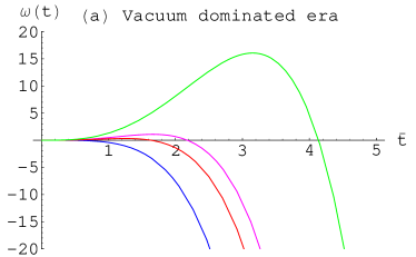
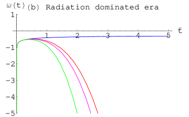
Figure 1: Plots show the graph of $\omega(t)$ versus cosmic time $t$ for (a) $\gamma=-1$ and (b) $\gamma=1/3$ with $\alpha=1.1$ and varying values of $\xi_{0}$ as follows: blue, $\xi_{0}=0.0001$; red, $\xi_{0}=0.15$; pink, $\xi_{0}=0.2$; green, $\xi_{0}=0.38$.

Now we discuss the BD parameter for vacuum as well as matter dominated eras. In the vacuum dominated era, the graphs indicate that $\omega(t)$ is a decreasing function starting from zero for $0<\xi_{0}\leq 0.11$. For $\xi_{0}>0.11$, the graphs correspond to increasing function but after some particular points, they again become decreasing function as shown in Figure 1. Thus, for this range of constant viscosity $\xi_{0}$ with $\alpha>1$, it is possible to achieve the cosmic acceleration with positive values of $\omega(t)$. In all other eras of the universe, $\omega(t)$ is a decreasing function of time with smaller negative values. For $0<\alpha<1$, in the radiation dominated era, $\omega(t)$ is a decreasing function and the universe undergoes to decelerated expansion. Thus, $\xi_{0}$ plays the role to control the time dependence of $\omega(t)$. In the radiation, matter dominated eras and massless scalar field, the BD parameter approaches to $-\infty$ for $\alpha=1/6,~{}1/3$ and $1/4$. For the cosmic acceleration, we must have $\alpha>1$, hence these values are not interesting.

3.2 Variable Bulk Viscosity Coefficient

For the sake of simplicity, we take $n=1/2$, i.e., $\xi(t,\rho)=\xi_{0}\rho^{1/2}(t)$. Using this value of bulk viscosity coefficient along with Eq.(13) in (11), it follows that

$$\dot{\rho(t)}+[\frac{3\alpha}{t}(1+\gamma)-\frac{9\xi_{0}\alpha^{2}}{t^{2}}]\rho(t)^{1/2}=0.$$

This yields the following solution

$$\rho(t)=\left[\frac{9\xi_{0}\alpha^{2}}{t[3\alpha(1+\gamma)-2]}+\rho_{0}t^{-3\alpha(1+\gamma)/2}\right]^{2},$$ (29)

where $\rho_{0}$ is an integration constant. Comparing this equation with Eq.(18), we obtain

$$\Omega(t)=3\left(\frac{2\alpha+\beta}{\beta}\right)^{2}-\frac{4t^{2}}{\phi_{0}\beta^{2}t^{\beta}}\left[\frac{9\xi_{0}\alpha^{2}}{t[3\alpha(1+\gamma)-2]}+\rho_{0}t^{-3\alpha(1+\gamma)/2}\right]^{2}.$$

The corresponding BD parameter will become

$$\omega(t)=-\frac{2t^{2}}{\phi_{0}\beta^{2}t^{\beta}}\left[\frac{9\xi_{0}\alpha^{2}}{t[3\alpha(1+\gamma)-2]}+\rho_{0}t^{-3\alpha(1+\gamma)/2}\right]^{2}.$$ (30)

For consistency of this solution with the wave equation, we substitute all these values in the wave equation (9) which leads to

$$\alpha=1/3,\quad\beta=-2\alpha,\quad\gamma=1.$$

For $\beta=-2\alpha$, we obtain

$$\omega(t)=-\frac{t^{2(1+\alpha)}}{2\phi_{0}\alpha^{2}}\left[\frac{9\xi_{0}\alpha^{2}}{t(3\alpha(1+\gamma)-2)}+\rho_{0}t^{-3\alpha(1+\gamma)/2}\right]^{2}.$$ (31)

The choice $\alpha=1/3$ is not feasible for obtaining cosmic acceleration while $\gamma=1$ corresponds to massless scalar field which is discussed below. Now we evaluate BD parameter for different eras.

In the vacuum dominated era, the BD parameter is

$$\omega(t)=-\frac{t^{2(1+\alpha)}}{2\phi_{0}\alpha^{2}}\left[\frac{-9\xi_{0}\alpha^{2}}{2t}+\rho_{0}\right]^{2}$$ (32)

while for the radiation dominated era, it turns out to be

$$\omega(t)=-\frac{t^{2(1+\alpha)}}{2\phi_{0}\alpha^{2}}\left[\frac{9\xi_{0}\alpha^{2}}{t(4\alpha-2)}+\rho_{0}t^{-2\alpha}\right]^{2}.$$ (33)

The BD parameter in the matter dominated era is

$$\omega(t)=-\frac{t^{2(1+\alpha)}}{2\phi_{0}\alpha^{2}}\left[\frac{9\xi_{0}\alpha^{2}}{t(3\alpha-2)}+\rho_{0}t^{-3\alpha/2}\right]^{2}.$$ (34)

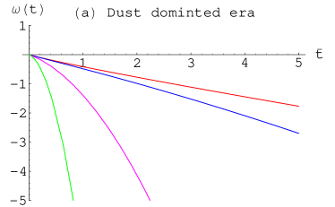
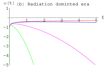
Figure 2: Plots show the graphs for $\omega(t)$ versus cosmic time $t$ for $\alpha=1.1$, (a) $\gamma=0$ and (b) $\gamma=1/3$ with varying values of $\xi_{0}$ as follows: red, $\xi_{0}=0.0001$; green, $\xi_{0}=0.38$; blue, $\xi_{0}=0.01$; pink, $\xi_{0}=0.1$.

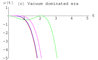
Figure 3: Plots shows the graphs for $\omega(t)$ versus cosmic time $t$ for $\alpha=1.1$ and $\gamma=-1$ with varying values of $\xi_{0}$ as follows: red, $\xi_{0}=0.0001$; green, $\xi_{0}=0.38$; blue, $\xi_{0}=0.01$; pink, $\xi_{0}=0.1$.

For the massless scalar field era, this is given by

$$\omega(t)=-\frac{t^{2(1+\alpha)}}{2\phi_{0}\alpha^{2}}\left[\frac{9\xi_{0}\alpha^{2}}{t(6\alpha-2)}+\rho_{0}t^{-3\alpha}\right]^{2}.$$ (35)

The expressions for $\omega(t)$ correspond to decreasing function as $-t^{2}$ for increasing values of viscosity coefficient $\xi_{0}$ and $-1\leq\gamma\leq 1$ except for vacuum dominated era. This gives rise to accelerated expansion of the universe for $\alpha>1$ as shown in Figures 2 and 3. For $\alpha=1/2,~{}3/2$ and $\alpha=1/3$, the BD parameter approaches to $-\infty$. Here in the matter dominated era, $\alpha=3/2$ lies in the range $\alpha>1$ allowed for the accelerated expansion of the universe.

Now we discuss the radiative fluid case ($n=1$). Here we take $\xi(t,\rho)=\xi_{0}\rho(t)$. Consequently, the continuity equation yields

$$\rho(t)=\rho_{0}t^{-3\alpha(1+\gamma)}\exp{(\frac{-9\xi_{0}\alpha^{2}}{t})}.$$ (36)

The BD parameter $\omega(t)$ turns out to be

$$\omega(t)=-\frac{2\rho_{0}\exp{(\frac{-9\xi_{0}\alpha^{2}}{t})}}{\phi_{0}\beta^{2}}t^{[(2-3\alpha(1+\gamma)-\beta]}.$$

Here $\beta=0$ and $\beta=-2\alpha$ are the corresponding consistency relations. The choice of $\beta=0$ provides no interesting insights while $\beta=-2\alpha$ leads to the following expression

$$\omega(t)=-\frac{\rho_{0}\exp{(\frac{-9\xi_{0}\alpha^{2}}{t})}}{2\phi_{0}\alpha^{2}}t^{[2-\alpha(1+3\gamma)]}.$$ (37)

For the radiation dominated era, the BD parameter takes the form

$$\omega(t)=-\frac{\rho_{0}\exp{(\frac{-9\xi_{0}\alpha^{2}}{t})}}{2\phi_{0}\alpha^{2}}t^{2(1-\alpha)}.$$ (38)

We see that the coefficient of viscosity appears only in the exponential function. Thus, in the radiation dominated era, for small values of $\xi_{0}$ and $\alpha>1,~{}\exp(-9\xi_{0}\alpha/t)\longrightarrow 1$, providing small negative values of $\omega(t)$ as shown in Figure 4. If $\xi_{0}\longrightarrow\infty$ with $\alpha>1$, then $\exp(-9\xi_{0}\alpha/t)\longrightarrow 0$ which means $\omega(t)\longrightarrow 0$. Thus this model may correspond to that of the metric $f(R)$ gravity. However, it is not physically possible. Also, in this case, for $0<\alpha<1$, the values of $\omega(t)$ are constrained within the range $-3/2<\omega(\phi)<0$ which shows that the universe undergoes to the decelerated phase.

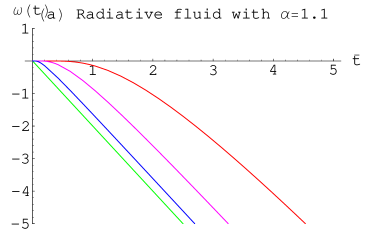
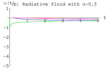
Figure 4: Plots show the graphs for $\omega(t)$ versus cosmic time $t$ for (a) $\alpha=1.1$ and (b) $\alpha=0.5$ with varying values of $\xi_{0}$ as follows: green, $\xi_{0}=0.0001$; red, $\xi_{0}=1.2$; blue, $\xi_{0}=0.09$; pink, $\xi_{0}=0.38$.

4 Cosmic Acceleration with Barotropic fluid and Bianchi I Universe Model

Here we investigate expansion of the universe by using LRS Bianchi type I model in the barotropic fluid background. The line element of Bianchi type I universe model is described by ⁴⁴⁾

$$ds^{2}=dt^{2}-A^{2}(t)dx^{2}-B^{2}(t)(dy^{2}+dz^{2}),$$ (39)

where $A$ and $B$ are the scale factors. This model has one transverse direction $x$ and two equivalent longitudinal directions $y$ and $z$. Assume that matter contents of the universe are described by the perfect fluid given by

$$T_{\mu\nu}=(\rho+P)u_{\mu}u_{\nu}-Pg_{\mu\nu}.$$ (40)

The corresponding field equations (2) and (3) can be written as

$$\frac{2\dot{A}\dot{B}}{AB}+\frac{\dot{B}^{2}}{B^{2}}=\frac{\rho}{\phi}+\frac{\omega(\phi)}{2}\frac{\dot{\phi}^{2}}{\phi^{2}}+\frac{V(\phi)}{2\phi}-(\frac{\dot{A}}{A}+2\frac{\dot{B}}{B})\frac{\dot{\phi}}{\phi},$$ (41)

$$2\frac{\ddot{B}}{B}+\frac{\dot{B}^{2}}{B^{2}}=-\frac{P}{\phi}-\frac{\omega(\phi)}{2}\frac{\dot{\phi}^{2}}{\phi^{2}}-2\frac{\dot{B}}{B}\frac{\dot{\phi}}{\phi}-\frac{\ddot{\phi}}{\phi}+\frac{V(\phi)}{2\phi},$$ (42)

$$\frac{\ddot{B}}{B}+\frac{\ddot{A}}{A}+\frac{\dot{A}\dot{B}}{AB}=-\frac{P}{\phi}-\frac{\omega(\phi)}{2}\frac{\dot{\phi}^{2}}{\phi^{2}}-\frac{\ddot{\phi}}{\phi}+\frac{V(\phi)}{2\phi}-(\frac{\dot{A}}{A}+\frac{\dot{B}}{B})\frac{\dot{\phi}}{\phi}.$$ (43)

The wave equation is

$$\ddot{\phi}+(\frac{\dot{A}}{A}+2\frac{\dot{B}}{B})\dot{\phi}=\frac{\rho-3P}{2\omega(\phi)+3}-\frac{[2V(\phi)-\phi\frac{dV(\phi)}{d\phi}]}{2\omega(\phi)+3}-\frac{\frac{d\omega(\phi)}{d\phi}\dot{\phi}^{2}}{2\omega(\phi)+3}.$$ (44)

For this model, the average scale factor and the mean Hubble parameter are

$$a^{3}(t)=AB^{2},\quad H(t)=\frac{1}{3}(\frac{\dot{A}}{A}+2\frac{\dot{B}}{B}).$$

The energy conservation equation for energy-momentum tensor given in Eq.(40) will be

$$\dot{\rho}+(\frac{\dot{A}}{A}+2\frac{\dot{B}}{B})(\rho+P)=0.$$ (45)

We assume that the universe is filled with barotropic fluid. The barotropic EoS ¹⁴⁾ is given by

$$P=\gamma\rho;\quad(-1\leq\gamma\leq 1).$$

The expansion scalar for Bianchi type I model is given by

$$\theta=u^{a}_{;a}=\frac{\dot{A}}{A}+2\frac{\dot{B}}{B}$$

while the shear scalar is

$$\sigma=\frac{1}{\sqrt{3}}(\frac{\dot{A}}{A}-\frac{\dot{B}}{B}).$$

It is given ⁴⁵⁾ that for spatially homogeneous metric, the normal congruence to homogeneous expansion yields the ratio $\frac{\sigma}{\theta}$ as constant i.e., ”expansion scalar $\theta$ is proportional to shear scalar $\sigma$”. This physical condition leads to the following relation between the scale factors

$$A=B^{m},$$ (46)

where $m\neq 1$ is any positive constant (for $m=1$, it reduces to flat FRW model). In literature ^44-49), this condition has been widely used to find exact cosmological models. Using this assumption in Eq.(45), it follows that

$$\dot{\rho}+(1+\gamma)(m+2)\frac{\dot{B}}{B}\rho(t)=0$$

which yields

$$\rho(t)=\rho_{0}B^{-(1+\gamma)(m+2)}.$$ (47)

Now we discuss the various possible choices for $\omega(\phi)$ and $V(\phi)$.

4.1 Model without potential $V(\phi)=0$

We take the following two cases according to $\omega$ is constant and $\omega=\omega(\phi)$.

4.1.1 Case (i)

First we take BD parameter as a constant, i.e., $\omega(\phi)=\omega_{0}$. For the solution of the field equations, we consider the power law as follows

$$B(t)=b_{0}t^{\alpha},\quad\alpha\geq 0.$$ (48)

Using Eqs.(46), (48) and the mean Hubble parameter $H$, the deceleration parameter can be written as

$$q=-[1-\frac{3}{\alpha(m+2)}].$$

Notice that $q<0,~{}q=0$ and $q>0$ indicate an accelerated expansion, uniform expansion and the decelerating phase of the universe respectively. Thus, for accelerated expansion of the universe, we must have the following condition on $\alpha$

$$\alpha>\frac{3}{(m+2)};\quad m\neq 1.$$ (49)

Substituting Eqs.(46) and (48) in (44), the scalar filed becomes

$$\phi(t)=\frac{(1-3\gamma)\rho_{0}b_{0}^{-(m+2)(1+\gamma)}t^{[2-\alpha(1+\gamma)(m+2)]}}{(3+2\omega_{0})[1-\alpha\gamma(m+2)][2-\alpha(1+\gamma)(m+2)]}.$$ (50)

The BD parameter is obtained from the field equations (41)-(43) as

$$\omega_{0} = -\frac{1}{(1-\gamma)}[\frac{(m+3)\alpha(\alpha-1)}{[2-\alpha(m+2)(1+\gamma)]^{2}}+\alpha^{2}\frac{[(m^{2}+1)+2\gamma(2m+1)]}{[2-\alpha(m+2)(1+\gamma)]^{2}}$$ (51)

$$+ \frac{\alpha[m+3+2\gamma(m+2)]}{[2-\alpha(m+2)(1+\gamma)]}+\frac{[1-\alpha(m+2)(1+\gamma)]}{[2-\alpha(m+2)(1+\gamma)]}].$$

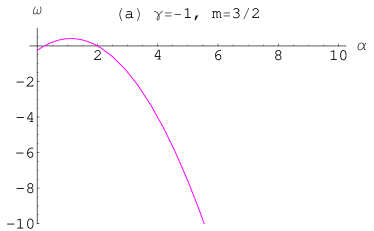
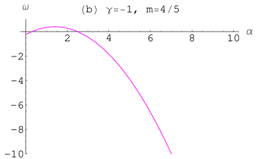
Figure 5: Plot of $\omega_{0}$ versus $\alpha$ for (a) $m=3/2$, (b) $m=4/5$ and $\gamma=-1$. The corresponding ranges for $\alpha$ are $\alpha>6/7$ and $\alpha>15/14$.

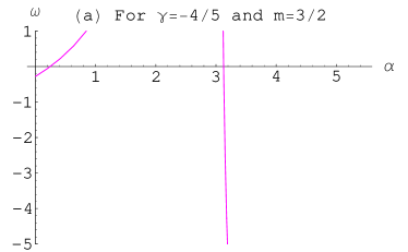
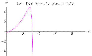
Figure 6: Plot of $\omega_{0}$ versus $\alpha$ for (a) $m=3/2$, (b) $m=4/5$ and $\gamma=-4/5$. The corresponding ranges for $\alpha$ are $\alpha>6/7$ and $\alpha>15/14$.

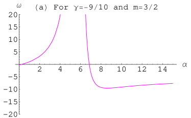
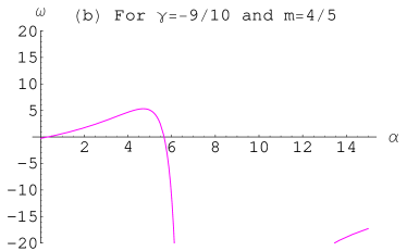
Figure 7: Plot of $\omega_{0}$ versus $\alpha$ for (a) $m=3/2$, (b) $m=4/5$ and $\gamma=-9/10$. The corresponding ranges for $\alpha$ are $\alpha>6/7$ and $\alpha>15/14$.

For massless scalar field $\gamma=1$, we have $\omega\longrightarrow-\infty$, which leads to GR. We have seen that the BD parameter depends upon the parameters $\alpha,~{}\gamma$ and $m$. These parameters are constrained using some physical conditions. The possible ranges for $m$ are $0<m<1$ and $m>1$ and $\gamma$ is allowed for $-1\leq\gamma\leq 1$. The deceleration parameter constraints $\alpha$ such that $\alpha>3/(m+2)$. By taking different possible choices for these parameters, it can be seen that BD parameter takes small negative values as well as positive values for $-1\leq\gamma<0$ as shown in Figures 5-7. This gives rise to cosmic acceleration for this range of $\gamma$. We would like to mention here that for ceratin ranges of $\alpha$ allowed for cosmic acceleration and $-1\leq\gamma<0,~{}\omega_{0}$ can take larger values which would be compatible with the solar system experiment constraints.

Solving Eq.(51) for $\alpha$, we obtain the following quadratic equation

$$\alpha^{2}[(m+2)^{2}(1+\gamma)^{2}[(\gamma-1)\omega_{0}-2]-(m+3)-[m^{2}+1+2\gamma(2m+1)]$$

$$+(m+2)(1+\gamma)[m+3+2\gamma(m+2)]]+\alpha[(m+2)(1+\gamma)[-4(\gamma-1)\omega_{0}$$

$$+6](m+3)-2[m+3+2\gamma(m+2)]]+4[\omega_{0}(\gamma-1)-1]=0$$ (52)

which provides two roots. These values for $m=1/2$ and $\gamma=0$ (present universe) are given by

$$\alpha=\frac{23/2+10\omega_{0}\pm\sqrt{-15/4-6\omega_{0}}}{17+25/2\omega_{0}}.$$ (53)

Since $-2\leq\omega_{0}\leq-3/2$ is the observed range for cosmic acceleration, so the choice of $\omega_{0}=-5/3$ leads to following values of $\alpha$

$$\alpha_{1}=16/23,\quad\alpha_{2}=2.$$

Here $\alpha_{1}$ gives $q>0$, hence we leave it while $\alpha_{2}=2$ yields $q<0$ leading to accelerating expansion. Also, it yields $\phi(t)=t^{-3}$ which provides positive coupling constant. Since in our case, $\phi(t)$ is decreasing more rapidly as compared to $\phi(t)=t^{-2}$ ¹¹⁾ and $\phi(t)=t^{-5/2}$ ¹²⁾, therefore it corresponds to greater rate of accelerated expansion of the universe.

4.1.2 Case (ii)

In this case, the BD parameter is not constant rather it is a function of $\phi$. Using Eqs.(13), (46), (41)-(43) and (48), the BD parameter can be written as

$$\omega(\phi) = \frac{1}{\beta^{2}}[\frac{(3m-m^{2}-2)}{2}\alpha^{2}+\frac{(m+3)\alpha}{2}+\frac{(m+1)\alpha\beta}{2}-\beta^{2}+\beta]$$ (54)

$$- \frac{1}{\beta^{2}}[\rho_{0}b_{0}^{-(m+2)(1+\gamma)}(1+\gamma)\phi^{\frac{-\alpha(m+2)(1+\gamma)-\beta+2}{\beta}}\phi_{0}^{\frac{-\alpha(m+2)(1+\gamma)-2}{\beta}}].$$

Substituting this value in Eq.(44), we obtain the following consistency relation

$$\beta=-\frac{(m+2)\alpha(1+\gamma)}{2};\quad m\neq 1$$ (55)

This shows that $\beta$ remains negative for all $0<m<1,~{}m>1$, $\alpha>3/(m+2)$ and $-1\leq\gamma\leq 1$. The consistency of this solution with the dynamical equations, i.e., each term in the dynamical equations should have the same time dependence, results in another constraint given by

$$\beta=2-\alpha(m+2)(1+\gamma).$$

Using this value of $\beta$ in Eq.(55), it can be seen that the parameter $\beta$ is restricted to $-2$. Now we discuss the BD parameter and cosmic acceleration in different phases of the universe by using this value of $\beta$. The expressions for BD parameter in matter and radiation dominated eras with $\beta=-2,~{}\alpha>6/5$ and $m=1/2$ turn out to be

$$\omega(\phi)=\frac{1}{4}[-\frac{3\alpha^{2}}{8}+\frac{\alpha}{4}-6]-\frac{1}{4}\phi^{(-2+\frac{5\alpha}{4})},$$

$$\omega(\phi)=\frac{1}{4}[-\frac{3\alpha^{2}}{8}+\frac{\alpha}{4}-6]-\frac{1}{3}\phi^{(-2+\frac{5\alpha}{3})}.$$

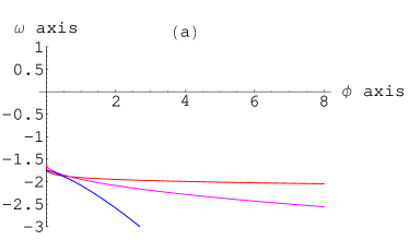
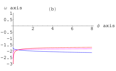
Figure 8: Plot of $\omega(\phi)$ versus $\phi$ for $m=1/2$ and (a) $\gamma=1/3$ and (b) $\gamma=0$ with $\alpha>6/5$ as follows: red, $\alpha=1.3$; blue, $\alpha=2$; pink, $\alpha=1.5$.

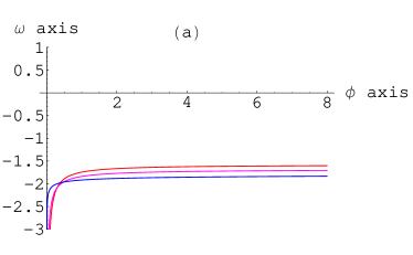
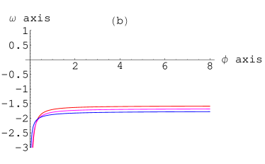
Figure 9: Plot of $\omega(\phi)$ versus $\phi$ for $m=1/2$ and (a) $\gamma=-1/3$ and (b) $\gamma=-1/2$ with $\alpha>6/5$ as follows: red, $\alpha=1.3$; blue, $\alpha=2$; pink, $\alpha=1.5$.

By taking different choices for these parameters, we see that for all phases of the universe, the BD parameter $\omega(\phi)$ has small negative values and lies within the range $\omega\leq-3/2$ as shown in Figures 8 and 9 which corresponds to accelerated expansion of universe. This result is in agreement with ¹⁴⁾ for spatially flat model.

4.2 Model with potential $V(\phi)\neq 0$

Again, we discuss two cases depending upon the value of BD parameter $\omega$.

4.2.1 Case (i)

First we discuss the case of constant BD parameter, i.e., $\omega(\phi)=\omega_{0}$. Further, we consider the power law form of the scalar field in terms of scale factor $B(t)$

$$\phi=\phi_{0}B^{\alpha};~{}~{}~{}\alpha>0.$$ (56)

Using this value of $\phi$ in the field equations (41)-(43), it follows that

$$\frac{\ddot{B}}{B}+A(\frac{\dot{B}^{2}}{B^{2}})=-CB^{-\alpha(1+\gamma)(m+2)},$$

where

$$A=\frac{(\alpha^{2}-3\alpha-2+2m^{2}+\alpha m-2m+\omega_{0}\alpha^{2})}{(3\alpha+2m)},~{}~{}C=\frac{(1+\gamma)\rho_{0}}{\phi_{0}(3\alpha+2m)}.$$

The expression for $\dot{B}(t)$ can be written as

$$\dot{B}(t) = \sqrt{\frac{2(1+\gamma)\rho_{0}}{\phi_{0}}}\times B(t)^{\frac{2-\alpha-(1+\gamma)(m+2)}{2}}\times[(3\alpha+2m)[(1+\gamma)(m+2)$$ (57)

$$+ (\alpha-2)]-2\alpha^{2}+6\alpha+4-4m^{2}-2m\alpha+4m-2\omega_{0}\alpha^{2}]^{-1/2}$$

which yields

$$B(t)=A^{\prime}t^{[2/[\alpha+(1+\gamma)(m+2)]},$$ (58)

where

$$A^{\prime} = [\frac{\rho_{0}}{2\phi_{0}}[\alpha+(1+\gamma)(m+2)]^{2}(1+\gamma)\times[(3\alpha+2m)[(1+\gamma)(m+2)+(\alpha$$

$$- 2)]-2\alpha^{2}+6\alpha+4-4m^{2}-2m\alpha+4m-2\omega_{0}\alpha^{2}]^{-1}]^{1/[\alpha+(1+\gamma)(m+2)]}.$$

The value of the scale factor $A(t)$ can be obtained by using value of $B(t)$ in Eq.(46).

The corresponding expression for the scalar field is given by

$$\phi(t)=\theta_{0}t^{2\alpha/[\alpha+(1+\gamma)(m+2)]},$$ (60)

where $\theta_{0}=\phi_{0}A^{\prime\alpha}$. Equation (58) yields the following constraint on $\alpha$

$$3\alpha\leq-(1+3\gamma)(m+2).$$ (61)

The deceleration parameter $q$ turns out to be

$$q=-1+\frac{3[\alpha+(1+\gamma)(m+2)]}{2(m+2)}.$$

It can be easily seen that for all positive constant $m$ ($m\neq 1$), $\alpha>1$ and $-1\leq\gamma\leq 1$, the deceleration parameter remains negative, i.e., $q<0$. Thus the universe is in the state of accelerated expansion. From the wave equation (44), the potential can be written as

$$V(\phi)=\frac{B^{\prime}}{\phi^{(1+\gamma)(m+2)/\alpha}},$$ (62)

where $B^{\prime}$ is given by

$$B^{\prime} = \frac{-\alpha\theta_{0}^{2/(\alpha p)}}{(1+\gamma)(m+2)[\alpha+(1+\gamma)(m+2)]^{2}}[4(1+\gamma)(m+2)(\omega_{0}\alpha$$

$$- m-2)-8(m+2)\alpha\omega_{0}+16m+8m^{2}+24-4m\alpha-8\alpha].$$

4.2.2 Case (ii)

Let us take the BD parameter as a function of the scalar field $\phi$, i.e, $\omega(\phi)$. Consider the power law forms for the scalar field and the scale factor, given by (48) and (13). Using the field equations (41)-(43), the scalar potential takes the form

$$V(\phi) = \phi_{0}^{(\frac{2}{\beta})}\phi^{\frac{(\beta-2)}{\beta}}[\frac{(m^{2}+5m+6)\alpha^{2}}{2}-\frac{(m+3)\alpha}{2}+\beta^{2}-\beta+(\frac{(3m+7)}{2})\alpha\beta]$$ (63)

$$- (1-\gamma)\rho_{0}b_{0}^{-(m+2)(1+\gamma)}\phi^{\frac{-\alpha(m+2)(1+\gamma)}{\beta}}\phi_{0}^{\frac{\alpha(m+2)(1+\gamma)}{\beta}}.$$

The BD parameter turns out to be the same as given by (54). Substituting these values in Eq.(44), we obtain the following consistency relations

$$\beta=0,\quad\beta=-2\quad\beta=-\frac{\alpha}{2}(m+3),\quad\beta=1-\alpha(m+2).$$ (64)

For the consistency of this solution with the dynamical equation, it follows that

$$\beta=2-\alpha(m+2)(1+\gamma).$$

Now we discuss the behavior of self-interacting potential $V(\phi)$ for these values of $\beta$ in different eras of the universe. The choice $\beta=0$ is not feasible, so we neglect it. For $\beta=-2$, the self-interacting potential can be written as

$$V(\phi)=\phi^{2}[(\frac{m^{2}+5m+6}{2})\alpha^{2}-(\frac{m+3}{2})\alpha+6-(3m+7)\alpha]-(1-\gamma)\phi^{\alpha(m+2)(1+\gamma)/2},$$

where $m\neq 1$ is a positive constant and $\alpha>3/(m+2)$. For $\beta=-\frac{9\alpha}{4},~{}m=3/2$ and $\alpha>6/7$, we get

$$V(\phi)=\phi^{(1+\frac{8}{9\alpha})}[-3\alpha^{2}]-(1-\gamma)\phi^{14(1+\gamma)/9}.$$

For $m=2,~{}\alpha>3/4$ and $\beta=-\frac{5\alpha}{2}$, the potential turns out to be

$$V(\phi)=-(1-\gamma)\phi^{8(1+\gamma)/5},$$

where $-1\leq\gamma\leq 1$.

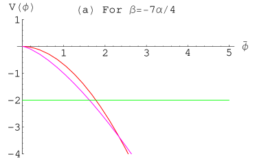
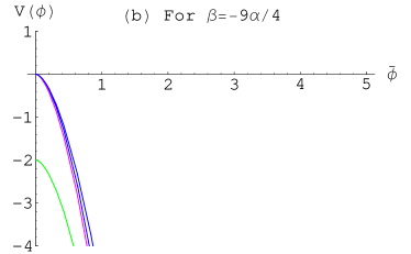
Figure 10: Plot (a) shows the graph of $V(\phi)$ versus scalar field $\phi$ for $m=1/2$, $\alpha=1.3$ and $\beta=-7\alpha/4$ as follows: red, $\gamma=1/3$; green, $\gamma=-1$; pink, $\gamma=0$ and Plot (b) shows the graph of $V(\phi)$ versus scalar field $\phi$ for $m=3/2$, $\alpha=1.3$ and $\beta=-9\alpha/4$ as follows: blue, $\gamma=1/3$; green, $\gamma=-1$; red, $\gamma=0$; pink, $\gamma=1$.

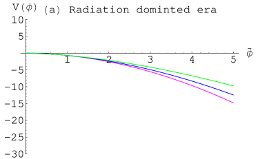
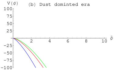
Figure 11: Plot (a) shows the graph of $V(\phi)$ versus scalar field for $m=1/2$, $\gamma=1/3$ and $\beta=1-5\alpha/2$ as follows: blue, $\alpha=1.5$; green, $\alpha=2$; pink, $\alpha=1.3$ and Plot (b) shows the graph of $V(\phi)$ versus scalar field for $m=3/2$, $\gamma=0$ and $\beta=1-7\alpha/2$ as follows: blue, $\alpha=2$; green, $\alpha=1.3$; red, $\alpha=1.5$.

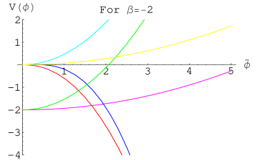
Figure 12: Plot shows the graph of $V(\phi)$ versus scalar field for $m=1/2$ and $\beta=-2$ as follows: blue, $\alpha=1.5$; red, $\alpha=1.3$ ($\gamma=1/3$); green, $\alpha=1.5$; pink, $\alpha=1.3$($\gamma=-1$); sky blue, $\alpha=1.5$; yellow, $\alpha=1.3$($\gamma=1$).

The expression for self-interacting potential for radiation dominated era with $\beta=2(1-\frac{5\alpha}{3}),~{}\alpha>6/5$ and $m=1/2$ is given by

$$V(\phi)=(\frac{95\alpha^{2}}{72}-\frac{13\alpha}{4}+\frac{4}{3})\phi^{\frac{-5\alpha/3}{(1-5\alpha/3)}}.$$

The self interacting potential for matter dominated era with $\beta=2-\frac{5\alpha}{2},~{}\alpha>6/5$ and $m=1/2$ takes the form

$$V(\phi)=(1-\frac{3\alpha}{4})\phi^{\frac{-5\alpha/2}{(2-5\alpha/2)}}.$$

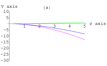
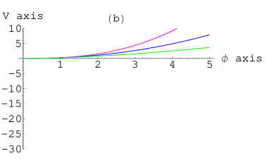
Figure 13: Plot (a) shows the graph of $V(\phi)$ versus scalar field for $m=1/2$, $\gamma=1/3$ and $\beta=2(1-5\alpha/3)$ as follows: blue, $\alpha=1.5$; green, $\alpha=2$; pink, $\alpha=1.3$ and Plot (b) shows the graph of $V(\phi)$ versus scalar field for $m=1/2$, $\gamma=0$ and $\beta=2-5\alpha/2$ as follows: blue, $\alpha=1.5$; green, $\alpha=2$; pink, $\alpha=1.3$.

For the first three consistency relations for $\beta$ given by Eq.(64), we see that $V(\phi)$ is a decreasing function starting from zero with the increasing values for $\phi$ except for the choice $\beta=-2$. In this case, only $\gamma=-1$ and $\gamma=1$ with $\alpha\geq 1.3$ provide positive potential energy as for these ranges, they are increasing functions of $\phi$ as shown in Figures 10-12. Figure 13(a) shows that $V(\phi)$ attains negative values starting from zero but with larger values for $\alpha$, it is an increasing function with positive values. Figure 13(b) shows that $V(\phi)$ attains positive increasing values for $\alpha>6/5$. Therefore, we conclude that these cases provide positive potential energy as they are increasing function of $\phi$ for particular values of $\alpha$.

5 Variation for the Newton’s Gravitational Constant in GBDT

A well-known fact about BD theory of gravity is that it provides very small variations for the gravitational constant. However, GBDT suggests various possibilities for variation of $G$. In GBDT, the expression for $G$ is found ²⁰⁾ to be

$$G(t)=\frac{4+2\omega(\phi)}{\phi(3+2\omega(\phi))}.$$

The present rate of variation for gravitational constant is given by

$$\left(\frac{\dot{G}}{G}\right)_{0}=-\left(\frac{\dot{\phi}}{\phi}\right)_{0}-\frac{2(\dot{\omega_{0}})}{(3+2\omega_{0})(4+2\omega_{0})}.$$ (65)

Here subscript indicates the present values of the corresponding parameters. Using Eq.(23), $\beta=-2\alpha,~{}\alpha>1,~{}\xi_{0}=0.0001$ and the estimated age of the universe $t_{0}=14\pm 2$ Gyrs, we obtain the rate of variation of $(\dot{G}/G)_{0}$ to be $1.5714\times 10^{-19}$ yrs. It lies clearly within the allowed range of variation of $G$ for cosmic acceleration, that is, $(\dot{G}/G)_{0}<4\times 10^{-10}$ yrs ^11,12).

For the Bianchi type $I$ model, by using expression for $\omega(\phi)$ given by Eq.(54) in Eq.(65) along with values $\beta=-2,~{}\alpha>6/5,~{}\gamma=0,~{}t_{0}=14\pm 2$ yrs and $m=1/2$, we obtain $(\dot{G}/G)_{0}=1.4287\times 10^{-10}$. It also safely lies within the allowed range of variation of $G$ for cosmic acceleration. Thus our obtained models satisfy the observational limit of $G$ for cosmic acceleration.

6 Summary and Discussion

This paper investigates the possibility of obtaining cosmic acceleration by using the role of BD parameter in the presence of viscous and barotropic fluids. For this purpose, we consider FRW and BI universe models. The constructed models entirely depend upon the values of the parameters $\alpha,~{}\beta,~{}\gamma$ and $m$. Firstly, we discuss the FRW model in the presence of viscous fluid. We see that the total effective pressure contains a negative factor associated with bulk viscosity which leads to negative effective pressure. Consequently, the fluid acts as a dark energy candidate and can explain many aspects of evolution of the universe. The deceleration parameter constraints the parameter $\alpha$ for cosmic acceleration i.e., $\alpha>1$.

For the constant coefficient of bulk viscosity, we obtain $\beta=0$ and $\beta=-2\alpha$. The first case leads to GR while for the second choice, in all eras of the universe except vacuum dominated era, the BD parameter $\omega(t)$ is a decreasing function of time with small negative values. In the vacuum dominated era, we see that for viscosity greater than $0.11$, it is possible to achieve cosmic acceleration with positive values of $\omega(t)$. For the variable bulk viscosity coefficient with $n=1/2,~{}\omega(t)$ corresponds to decreasing function as $-t^{2}$ with small negative values for different small values of viscosity coefficient $\xi_{0}$ and $-1\leq\gamma\leq 1$. This gives rise to accelerated expansion of the universe for $\alpha>1$. For the radiative fluid, we have found that the coefficient of viscosity appears in exponential function. Here $\omega(t)$ is a decreasing function with negative values both for the accelerated and decelerated phases of the universe ($-3/2\leq\omega\leq 0$).

Secondly, we have taken the BI universe model in the presence of perfect fluid with barotropic EoS. Here we have taken two cases when $V(\phi)=0$ and $V(\phi)\neq 0$. In the first case, when $\omega(\phi)=\omega_{0}$, by taking different possible choices for the parameters, we see that the BD parameter takes small negative as well as positive values for $-1\leq\gamma<0$ and certain ranges of $\alpha$. Thus the cosmic acceleration can be achieved for positive larger values of $\omega$ with different values of $\alpha$. Also, for the present universe with $\omega_{0}=-5/3$ (taken from the negative observed range for cosmic acceleration $-2\leq\omega_{0}\leq-3/2$), we have found $\phi(t)\sim t^{-3}$. In this case, the acceleration rate of the universe is higher than Bertolami et al. $(\phi(t)\sim t^{-2})$ ¹¹⁾ and Benerjee et al. $(\phi(t)\sim t^{-5/2})$ ¹²⁾. When $\omega=\omega(\phi)$, taking different values of the parameters, we see that for all phases of the universe, the BD parameter $\omega(\phi)$ have small negative values and lies within the range $\omega\leq-3/2$ which corresponds to cosmic acceleration and in agreement with already found results ¹⁴⁾.

For $V(\phi)\neq 0$ and $\omega(\phi)=\omega_{0}$, we have evaluated the values of scale factors $A$, $B$, scalar field and $V(\phi)$. It is found that in all phases of the universe, these values of scale factors $A(t)$ and $B(t)$ lead to $q<0$ for all positive constant $m$ with $m\neq 1$ and $\alpha>1$ which corresponds to cosmic acceleration. Finally, for $V(\phi)\neq 0$ and $\omega=\omega(\phi)$, we see that $V(\phi)$ is a decreasing function starting from zero with the increasing $\phi$ except for the choice $\beta=-2$ with particular values of $\gamma$ and $\alpha\geq 1.3$. These values provide positive potential energy as they are increasing function of $\phi$. However, for the constraint $\beta=2-\alpha(m+2)(1+\gamma)$, it is possible to have positive potential energy for larger values of $\alpha$ in matter dominated era while for smaller values of $\alpha$ in radiation dominated era.

It is worthwhile to mention here that all models discussed here satisfy the observational constraints for the variation of Newton’s gravitational constant available in literature ^11,12) which provides a support to our obtained results. Although in each case, we have explained the phenomena of cosmic acceleration for different ranges of the corresponding parameters. However, these ranges of the BD parameter, except for few cases, are incompatible with solar system constraints which require $\omega\geq 40,000$. This is the generic problem noted in the context of scalar tensor theories. It would be of great interest to see whether this problem can be resolved using other Bianchi models.

In order to check the viability of dark energy models based on modified theories of gravity, the evolution of cosmological perturbations and the background expansion history of the universe may be studied. This can be done through Chameleon and Vainshtein mechanisms which suppress the propagation of fifth force and provide consistency with local gravity experiments ^50,51). One may adopt these procedures to check the viability of above discussed models.

1) S. Perlmutter, S. Gabi, G. Goldhaber, A. Goobar, D. E. Groom, I. M. Hook, A. G. Kim, M. Y. Kim, G. C. Lee, R. Pain, C. R. Pennypacker, I. A. Small, R. S. Ellis, R. G. McMahon, B. J. Boyle, P. S. Bunclark, D. Carter, M. J. Irwin, K. Glazebrook, H. J. M. Newberg, A. V. Filippenko, T. Matheson, M. Dopita and W. C. Couch: Astrophys. J. 483(1997)565; S. Perlmutter, G. Aldering, M. D. Valle, S. Deustua, R. S. Ellis, S. Fabbro, A. Fruchter, G. Goldhaber, A. Goobar, D. E. Groom, I. M. Hook, A. G. Kim, M. Y. Kim, R. A. Knop, C. Lidman, R. G. McMahon, P. Nugent, R. Pain, N. Panagia, C. R. Pennypacker, P. Ruiz-Lapuente, B. Schaefer and N. Walton: Nature 391(1998)51; S. Perlmutter, G. Aldering, G. Goldhaber, R. A. Knop, P. Nugent, P. G. Castro, S. Deustua, S. Fabbro, A. Goobar, D. E. Groom, I. M. Hook, A. G. Kim, M. Y. Kim, J. C. Lee, N. J. Nunes, R. Pain, C. R. Pennypacker, R. Quimbey, C. Lidman, R. S. Ellis, M. Irwin, R. G. Mcmahon, P. Ruiz-lapuente, N. Walton, B. Schaefer, B. J. Boyle, A. V. Filippenko, T. Matheson, A. S. Fruchter, N. Panagia, H. J. M. Newberg and W. J. Couch: Astrophys. J. 517(1999)565.
2) A. G. Riess, A. V. Filippenko, P. Challis, A. ClocChiatti, A. Diercks, P. M. Garnavich, R. L. Gilliland, C. J. Hogan, S. Jha, R. P. Kirshner, B. Leibundgut, M. M. Phillips, D. Reiss, B. P. Schmidt, R. A. Schommer, R. C. Smith, J. Spyromilio, C. Stubbs, N. B. Suntzeff and J. Tonry: Astron. J. 116(1998)1009.
3) C. L. Bennett, M. Halpern, G. Hinshaw, N. Jarosik, A. Kogut, M. Limon, S. S. Meyer, L. Page, D. N. Spergel, G. S. Tucker, E. Wollack, E. L. Wright, C. Barnes, M. R. Greason, R. S. Hill, E. Komatsu, M. R. Nolta, N. Odegard, H. V. Peiris, L. Verde and J. L. Weiland: Astrophys. J. Suppl. 148(2003)1.
4) M. Tegmark, M. A. Strauss, M. R. Blanton, K. Abazajian, S. Dodelson, H. Sandvik, X. Wang, D. H. Weinberg, I. Zehavi, N. A. Bahcall, F. Hoyle, D. Schlegel, R. Scoccimarro, M. S. Vogeley, A. Berlind, T. Budavari, A. Connolly, D. J. Eisenstein, D. Finkbeiner, J. A. Frieman, J. E. Gunn, L. Hui, B. Jain, D. Johnston, S. Kent, H. Lin, R. Nakajima, R. C. Nichol, J. P. Ostriker, A. Pope, R. Scranton, U. Seljak, R. K. Sheth, A. Stebbins, A. S. Szalay, I. Szapudi, Y. Xu, J. Annis, J. Brinkmann, S. Burles, F. J. Castander, I. Csabai, J. Loveday, M. Doi, M. Fukugita, B. Gillespie, G. Hennessy, D. W. Hogg, Z. E. Ivezic , G. R. Knapp, D. Q. Lamb, B. C. Lee, R. H. Lupton, T. A. McKay, P. Kunszt, J. A. Munn, L. Connell, J. Peoples, J. R. Pier, M. Richmond, C. Rockosi, D. P. Schneider, C. Stoughton, D. L. Tucker, D. E. V. Berk, B. Yanny and D. G. York: Phys. Rev. D69(2004)03501.
5) S. W. Allen, R. W. Schmidt, H. Ebeling, A. C. Fabian and L. V. Speybroeck: Mon. Not. Roy. Astron. Soc. 353(2004)457.
6) E. Hawkins, S. Maddox, S. Cole, O. Lahav, D. S. Madgwick, P. Norberg, J. A. Peacock, I. K. Baldry, C. M. Baugh, J. Bland-Hawthorn, T. Bridges, R. Cannon, M. Colless, C. Collins, W. Couch, G. Dalton, R. D. Propris, S. P. Driver, S.P., G. Efstathiou, R. S. Ellis, C.S. Frenk, K. Glazebrook, C. Jackson, B. Jones, I. Lewis, S. Lumsden, W. Percival, B. A. Peterson, W. Sutherland and K. Taylor: Mon. Not. Roy. Astr. Soc. 346(2003)78.
7) B. Jain and A. Taylor: Phys. Rev. Lett. 91(2003)141302.
8) R. R. Caldwell, R. Dave and P. J. Steinhardt: Phys. Rev. Lett. 80(1998)1582.
9) A. S. Al-Rawaf and M. O. Taha: Gen. Relativ. Gravit. 28(1996)935.
10) A. H. Guth: Phys. Rev. D23(1981)347.
11) O. Bertolami and P. J. Martins: Phys. Rev. D61(2000)064007.
12) N. Banerjee and D. Pavon: Phys. Rev. D63(2001)043504.
13) B. K. Sahoo and L. P. Singh: Mod. Phys. Lett. A18(2003)2725.
14) W. Chakraborty and U. Debnath: Int. J. Theor. Phys. 48(2009)232.
15) C. H. Brans and R. H. Dicke: Phys. Rev. 124(1961)925.
16) S. Weinberg: Gravitation and Cosmology (Wiley, 1972).
17) P. A. M. Dirac: Proc. R. Soc. Lond. A165(1938)199.
18) B. Bertotti, L. Iess and P. Tortora: Nature 425(2003)374.
19) A. D. Felice, G. Mangano, P. D. Serpico and M. Trodden: Phys. Rev. D74(2006)103005.
20) K. Nordtvedt Jr.: Astrophys. J. 161(1970)1059.
21) R. V. Wagoner: Phys. Rev. D1(1970)3209.
22) T. Singh and L. N. Rai: Gen. Relativ. Gravit. B15(1983)875.
23) M. S. Bermann: Nuovo Cimento B74(1983)192.
24) S. Sen and A. A. Sen: Phys. Rev. D63(2001)124006.
25) B. K. Sahoo and L. P. Singh: Mod. Phys. Lett. A17(2002)2409.
26) S. Sen and T. R. Seshadri: Int. J. Mod. Phys. D12(2003)445.
27) D. R. K. Reddy and M. V. S. Rao: Astrophys. Space. Sci. 305(2006)183.
28) J. P. Singh and P. S. Baghel: Elect. J. Theor. Phys. 6(2009)85.
29) M. K. Verma, M. Zeyauddin and S. Ram: Rom. J. Phys. 56(2011)616.
30) M. Sharif and S. Waheed: Eur. Phys. J. 72C(2012)1876; A. K. Yadav and B. Saha: Astrophys. Space. Sci 337(2012)759.
31) C. P. Singh: Brazil. J. Phys. 39(2009)619.
32) S. Fay: Gen. Relativ. Gravit. 32(2000)203.
33) S. K. Rama and S. Gosh: Phys. Lett. B383(1996)32; S. K. Rama: Phys. Lett. B373(1996)282.
34) C. Romero and A. Barros: Phys. Lett. A173(1993)243.
35) N. Banerjee and S. Sen: Phys. Rev. D56(1997)1334.
36) A. Bhadra and K. K. Nandi: Phys. Rev. D64(2001)087501.
37) C. H. Brans: Phys. Rev. 125(1962)2194.
38) T. P. Sotiriou and V. Faraoni: Rev. Mod. Phys. 82(2010)451.
39) C. Eckart: Phys. Rev. 58(1940)919.
40) G. L. Murphy: Phys. Rev. D8(1973)4231.
41) S. Weinberg: Astrophys. J. 168(1971)175.
42) U. A. Belinskii and I. M. Khalatnikov: Sov. Phys. JETP 42(1976)205.
43) G. P. Singh, S. G. Ghosh and A. Beesham: Aust. J. Phys. 50(1997)903.
44) M. Sharif and M. Zubair: Astrophys. Space Sci. 330(2010)399.
45) C. B. Collins, E. N. Glass and D. A. Wilkinson: Gen. Relativ. Gravit. 12(1980)805.
46) K. S. Throne: Astrophys. J. 148(1967)51.
47) J. Kristian and R. K. Sachs: Astrophys. J. 143(1966)379.
48) C. B. Colins: Phys. Lett. A60(1977)397.
49) S. R. Roy and S. K. Banerjee: Class. Quantum Grav. 11(1995)1943.
50) G. Radouane, M. Bruno, F. M. David, P. David, T. Shinji and A. W. Hans: Phys. Rev. D82(2010)124006.
51) T. Shinji: Lect. Notes Phys. 800(2010)99.