Aberration-corrected quantum temporal imaging system

Abstract

We describe the design of a temporal imaging system that simultaneously reshapes the temporal profile and converts the frequency of a photonic wavepacket, while preserving its quantum state. A field lens, which imparts a temporal quadratic phase modulation, is used to correct for the residual phase caused by field curvature in the image, thus enabling temporal imaging for phase-sensitive quantum applications. We show how this system can be used for temporal imaging of time-bin entangled photonic wavepackets and compare the field lens correction technique to systems based on a temporal telescope and far-field imaging. The field-lens approach removes the residual phase using four dispersive elements. The group delay dispersion (GDD) $D$ is constrained by the available bandwidth $\Delta\nu$ by $D>t/\Delta\nu$, where $t$ is the temporal width of the waveform associated with the dispersion $D$. This is compared to the much larger dispersion $D\gg\pi t^{2}/8$ required to satisfy the Fraunhofer condition in the far field approach.

PACS numbers

03.65.Wj, 03.65.Ud, 03.67.Hk, 03.67.Mn

I Introduction

Quantum communication systems rely on transforming and transmitting information using quantum systems, such as atoms, trapped ions and photons Gisin et al. (2002); Leibfried et al. (2003); Gisin and Thew (2007); Kimble (2008); Raymer and Srinivasan (2012). It is widely believed that future quantum information system will consist of more than one type of physics system Gisin and Thew (2007); Kimble (2008); Raymer and Srinivasan (2012); Leibfried et al. (2003), such hybrid quantum connections have been demonstrated between ion and photon Stute et al. (2013) and proposed for atoms and quantum dots Waks and Monroe (2009). In hybrid systems, photons are often used as propagating quantum information carrier, or flying qubits, to connect different quantum systems Kim et al. (2011); Cirac et al. (1997). In long-distance quantum communication between hybrid quantum platforms, the wavelength, temporal scale and spectral profile of the photonic wave-packet for the source and target quantum memories and transmission channel are very different Raymer and Srinivasan (2012). We need an efficient interface to convert the wavelengths and temporal scales of the photonic wave packet to match quantum memories, while preserving the quantum state. Here, we propose a quantum interface for flying qubits (photons) using temporal imaging integrated with nonlinear optical wavelength conversion.

The bridge between different wavelengths has been intensely investigated in the quantum optics field. Quantum connections are generated either via broadband entangled photon pair sources Söller et al. (2010), or via nonlinear frequency conversion of the photonic wavepacket Kumar (1990); Huang and Kumar (1992); Albota and Wong (2004); Langrock et al. (2005); VanDevender and Kwiat (2007); Pelc et al. (2011); Rakher et al. (2010); Shahriar et al. (2012); Mejling et al. (2012); McKinstrie et al. (2005a, b); McGuinness et al. (2010). Preserving the quantum state is achieved using nonlinear frequency conversion processes that do not amplify the input state (which adds noise), such as three-wave mixing (3WM) Kumar (1990); Huang and Kumar (1992); Albota and Wong (2004); Langrock et al. (2005); VanDevender and Kwiat (2007); Pelc et al. (2011); Rakher et al. (2010); Shahriar et al. (2012) and Bragg-scattering-type four-wave mixing Clemmen et al. (2012); Mejling et al. (2012); McKinstrie et al. (2005a, b); McGuinness et al. (2010). In these schemes, the quantum state of the signal beam is transferred to the idler beam at full conversion without excess noise McKinstrie et al. (2005b). Additionally, the phase of the pump beam is impressed onto the generated idler waveform McGuinness et al. (2010), enabling engineered phase modulation of the wavepacket.

At the same time, researchers have been investigating temporal reshaping of photonic wavepacket, while preserving its quantum states Pe’Er et al. (2005); Kielpinski et al. (2011); Brecht et al. (2011); McKinstrie et al. (2012). Kielpinski et al. propose to use a well designed frequency-dependent dispersion function and temporal phase modulation to reconstruct the pulse shape Kielpinski et al. (2011). McKinstrie et al. suggest reshaping the signal pulse profile using pump pulse that has slight mismatch in group velocity McKinstrie et al. (2012). Both proposed schemes requires tailored dispersion functions that are highly depended on the details of original pulse shape.

Temporal imaging techniques have been developed by the ultrafast optics laser community for temporal rescaling of optical pulses Kolner and Nazarathy (1989); Tsang and Psaltis (2006); Salem et al. (2008); Foster et al. (2009, 2008). They are the temporal analog of spatial imaging systems. As shown in Fig. 1, in a single-lens spatial imaging system, spatial Fourier components of light waves scattered from the object diffract into different angular directions. A lens encodes a quadratically-varying phase to each of these components according to the direction. The resulting Fourier components then diffract and recombine to form an image at the image plane. In a temporal imaging system, temporal Fourier components of light waves are dispersed into different temporal locations upon propagating in a medium characterized by a non-zero group velocity dispersion. The dispersed (or chirped) light wave is modulated by a temporally-varying quadratic phase, known as a “time lens.” Similarly, a temporal “image” is formed after a second dispersive medium recombines (or dechirps) the Fourier components in time.

Here, we combine temporal imaging with a nonlinear frequency conversion process that is pumped by a chirped pulse with a quadratically varying phase profile, which imposes the necessary time lens phase modulation. In this way, we realize wavelength conversion and temporal imaging simultaneously.

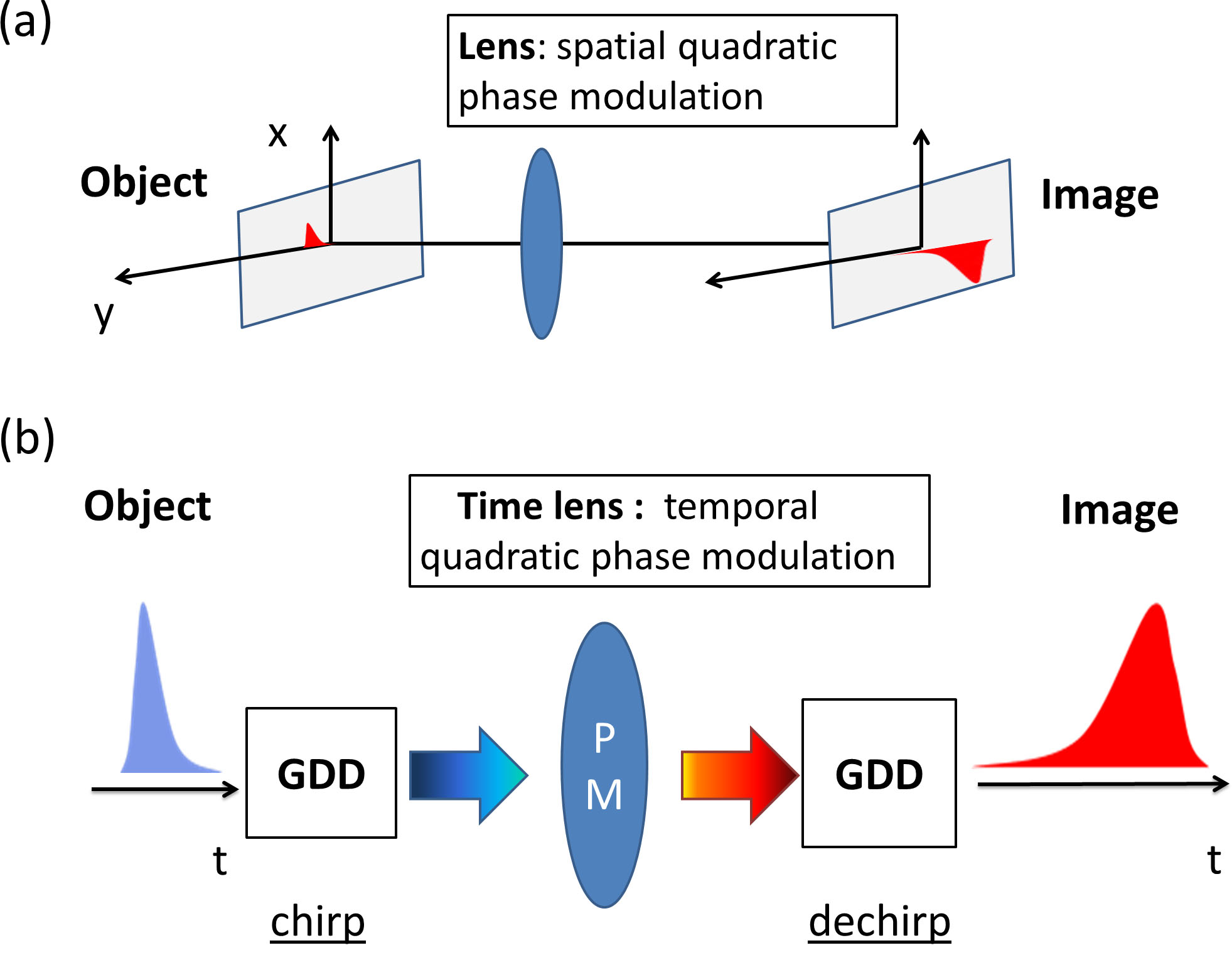
Figure 1: Analog of spatial (a) and temporal (b) imaging system. GDD: group delay dispersion, PM: phase modulation

In a spatial single-lens imaging system, it is well known that a residual quadratic phase is present at the image even if the intensity profile is aberration free. Similarly, a residual phase remains in a single-lens temporal imaging system. In most classical ultrafast laser applications where only the intensity of the waveform is detected, residual phase plays no significant role. However, the phase of the photonic wavepacket is an essential feature in most quantum applications, such as in conventional phase-encoded quantum key distribution systems, where the complete two-dimensional Hilbert space is used for information processing Gisin and Thew (2007). In these applications, it is highly desirable that this phase be compensated.

In this paper, we present a solution to the residual phase problem by adding a field lens to the imaging system. We describe the properties of this imaging system for the case of a time-bin entangled photonic wavepacket and compare the field-lens technique with other solutions that are based on temporal telescopes and far-field imaging. We find that the field-lens approach has better performance with less dispersion and a simpler setup. The field lens approach uses only four dispersive elements. The requirement for group delay dispersion (GDD) $D$ becomes $D>t/\Delta\nu$, where $t$ is the temporal width of the waveform associated with the dispersion $D$. Compared to the Fraunhofer condition $D\gg\pi t^{2}/8$ in the far field approach, the dispersion requirement is dramatically reduced. As a result, inherent loss in the dispersive elements is also reduced. This method thus paves the way toward the development of a highly efficient and flexible flying qubit interface.

II Quantum theory for temporal imaging systems

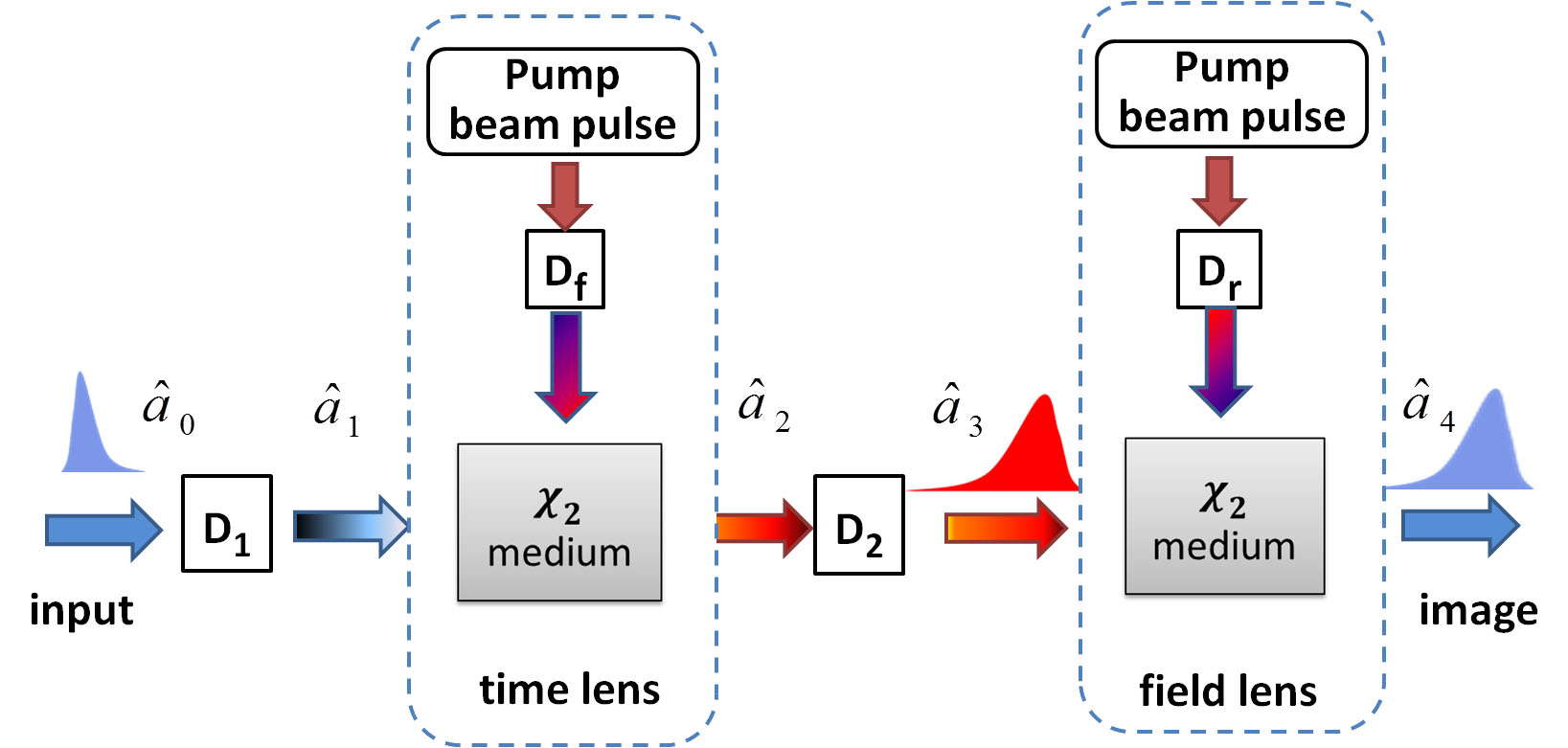
Figure 2: Abberation-corrected flying qubit interface consists of a single-lens imaging system and a field lens

II.1 System design overview

The flying qubit interface consists of a single-lens imaging system and a field lens placed in the image plane, as shown in Fig. 2. An input wavepacket (denoted by the annihilation operator $\hat{a}_{0}$) first propagates through a dispersive medium $D_{1}$. The dispersed wavepacket $\hat{a}_{1}$ then enters the time lens, which is constructed using a 3WM process in a crystal with a second-order nonlinear optical susceptibility $\chi_{2}$. The beam that pumps the 3WM process (field $E_{p}$) has a quadratic phase $\phi_{p}$ obtained upon propagating through another dispersive material $D_{f}$, which is encoded on the generated waveform $\hat{a}_{2}$ in the 3WM frequency down-conversion process. The phase-modulated wavepacket $\hat{a}_{2}$ then propagates through dispersive medium $D_{2}$ to dechirp (into $\hat{a}_{3}$). Finally, a field lens (with quadratic phase $\phi^{\prime}_{p}$ on the pump filed $E_{p}^{\prime}$ obtained from dispersion $D_{r}$) frequency up-converts the wavepacket and removes the residual phase $\theta_{r}$. We obtain a chirp free temporal image wavepacket $\hat{a}_{4}$. Here all $D$’s are the group delay dispersion $D=\beta_{2}L$, where $\beta_{2}$ and $L$ are the group velocity dispersion (GVD) parameter and length of the dispersive material, respectively.

II.2 Quantum description of light propagating in a dispersive material

To explore the evolution of the annihilation operator $\hat{a}$ for a photonic wavepacket propagating along the $+z$ direction in a dispersive material, we expand the operator in the temporal $t$ and frequency $\omega$ domains as Loudon (2000)

$$\hat{a}=\int dt\ \hat{a}(t)=\int d\omega\ {\hat{a}}(\omega),$$ (1)

where $\hat{a}(t)$ and ${\hat{a}}(\omega)$ are Fourier transform pairs and are the temporal and spectral profile annihilation operators of the mode, respectively. Dispersive propagation is best described in the frequency domain and is governed by Loudon (2000)

$$\frac{\partial\hat{a}(z,\omega)}{\partial z}=\imath\frac{\omega n(\omega)}{c}\hat{a}(z,\omega),$$ (2)

where $c$ is the speed of light in vacuum, and $n$ is the refractive index of the material. For the case of small dispersion, $\omega n(\omega)/c$ is expanded around the carrier frequency $\omega_{0}$ as

$$\omega n(\omega)/c\approx\beta_{0}+\beta_{1}(\omega-\omega_{0})+\frac{\beta_{2}}{2}(\omega-\omega_{0})^{2}+...,$$ (3)

where $\beta_{i}=\partial^{i}(\omega n(\omega)/c)/\partial\omega^{n}|_{\omega=\omega_{0}}$.

To second-order in the dispersion and ignoring absorption, the solution to the evolution equation Eq. (2) is given by

$$\hat{a}(z,\omega)=\hat{a}(0,\omega)e^{\imath(1/2){\beta_{2}}(\omega-\omega_{0})^{2}z},$$ (4)

when moving in a reference frame traveling at speed $1/\beta_{1}$.

We therefore obtain the results that

$$\hat{a}_{1}(\omega)=\hat{a}_{0}(\omega)e^{\imath(1/2){D_{1}}(\omega-\omega_{0})^{2}},$$ (5)

and

$$\hat{a}_{3}(\omega)=\hat{a}_{2}(\omega)e^{\imath(1/2){D_{2}}(\omega-\omega_{0})^{2}}.$$ (6)

II.3 Quantum theory of the time lens using the 3WM process

The time lens is constructed using a 3WM process in a $\chi_{2}$ crystal. When pumped by a strong (classical) beam $E_{p}(t)=A_{p}(t)e^{\imath\phi_{p}(t)}$ ($A_{p}$ and $\phi_{p}$ being the amplitude and phase of the pump beam, respectively), the mode occurrence probability oscillates back and forth between the two co-propagating signal ($\hat{a}_{s}$) and idler ($\hat{a}_{i}$) beams as a result of sum-frequency and difference-frequency generation (SFG and DFG). When the phase matching conditions of frequency $\omega$ and wavevector $k$

$$\omega_{i}=\omega_{s}+\omega_{p}$$

$$k_{i}=k_{s}+k_{p}$$

are fulfilled, the Hamiltonian for the process is expressed as Boyd (2003)

$$H=\int dt\ {\gamma E_{p}(t){a}_{s}^{\dagger}(t)\hat{a}_{i}(t)+c.c.},$$ (7)

where the nonlinear coefficient $\gamma$ is proportional to $\chi_{2}$. Note the pump is assumed to not be depleted and thus $E_{p}$ remains unchanged throughout the process.

Solving the evolution equations of the wavepacket operators, namely

$$\partial\hat{a}_{s}/\partial z=\imath[\hat{a}_{s},H],$$

$$\partial\hat{a}_{i}/\partial z=\imath[\hat{a}_{i},H],$$

we find that the mode occurrence probabilities oscillate with the pump amplitude. Particularly, when the $A_{p}$ reaches the critical value so that $\gamma A_{p}L_{c}=\pi/2$, where $L_{c}$ is the length of the crystal, the conversion efficiency becomes 100% and the optical field switches between two frequency modes, as expressed by

$$\hat{a}_{i}(z,t)=\imath\hat{a}_{s}(0,t)e^{\imath\phi_{p}(t)}$$

$$\hat{a}_{s}(z,t)=\imath\hat{a}_{i}(0,t)e^{-\imath\phi_{p}(t)}$$

By using such a non-amplifying process, the quantum state of the input signal waveform is transformed to the idler beam (or vice versa) and the phase (or conjugated phase) from the pump pulse is imposed onto the output beam as well McKinstrie et al. (2005b, a).

The result is applied to the time lens sections in the imaging systems. For the down-conversion time lens

$$\hat{a}_{2}(t)=\imath e^{-\imath\phi_{p}(t)}\hat{a}_{1}(0,t),$$ (9)

and for the up-conversion field lens

$$\hat{a}_{4}(t)=\imath e^{\imath\phi_{p}^{\prime}(t)}\hat{a}_{3}(0,t).$$ (10)

II.4 A single-lens temporal imaging system with residual phase

We now consider the single-lens temporal imaging system with two dispersive elements ($D_{1}$, $D_{2}$) and a time lens (characterized by $D_{f}$). The pump pulse $E_{p}(t)=A(t)e^{\phi_{p}(t)}$ has a quadratic phase $\phi_{p}(t)=t^{2}/2D_{f}$, generated via propagating a short pulse through a dispersive element with total dispersion $D_{f}$ Boyd (2003).

Combining Eq. (5-6) and Eq. (9), the output wavepacket $\hat{a}_{3}(\omega)$ at the image plane is expressed in terms of input wavepacket $\hat{a}_{0}(\omega)$ by

$$\hat{a}_{3}(\omega)= e {}^{\imath[D_{2}(\omega-\omega_{0})^{2}/2]}\int dte^{-\imath\omega t}e^{-\imath t^{2}/2D_{f}}$$ (11)

$$\int d\omega^{\prime}e^{\imath\omega^{\prime}t}\hat{a}_{0}(\omega^{\prime})e^{\imath[D_{1}(\omega^{\prime}-\omega_{0})^{2}/2]},$$

Carrying out the integration over $t$, we obtain

$$\hat{a}_{3}(\omega)= e {}^{\imath[D_{2}(\omega-\omega_{0})^{2}/2]}$$ (12)

$$\int d\omega^{\prime}\ e^{\imath[-D_{f}(\omega-\omega^{\prime})^{2}/2+D_{1}\omega^{\prime 2}/2]}\hat{a}_{0}(\omega^{\prime}).$$

When the imaging conditions

$$1/D_{1}+1/D_{2} = 1/D_{f}$$

$$-D_{2}/D_{1} = M$$ (13)

are fulfilled, taking a Fourier transform of $\hat{a}_{3}(\omega)$ and carrying out the integration over $\omega$, result in the simplified expression

$$\hat{a}_{3}(t)=\frac{\imath}{\sqrt{M}}\hat{a}_{0}(0,\frac{t}{M})e^{\imath\theta_{r}(t)},$$ (14)

where the output temporal profile is magnified by a factor $M$ and a quadratic phase $\theta_{r}=t^{2}/(2MD_{f})$ is left in the waveform.

III Residual phase correction schemes and comparison

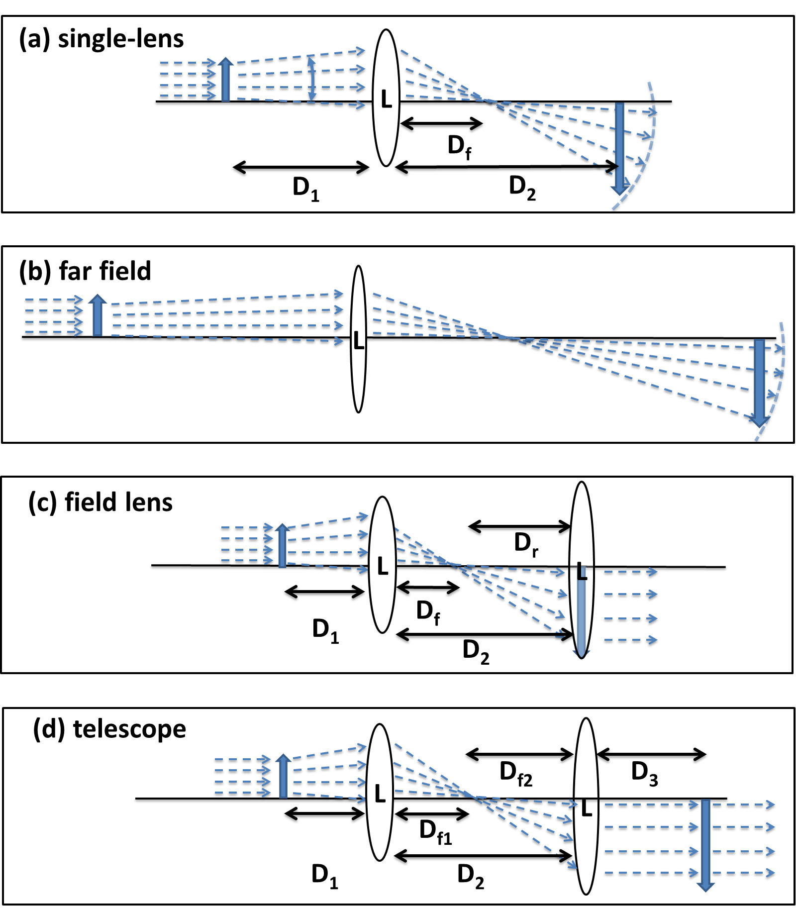
Figure 3: Residual phase in a spatial imaging system and three configurations to correct for it. Here, $D$ represents diffraction, which is proportional to the distance between each elements. Figure (a) shows the original single-lens system with image-plane curvature, (b) far-field imaging with reduced Petzval field curvature, (c) an imaging system with a field lens in the image plane and (d) a telescope imaging systems with no field curvature.

The quadratic residual phase $\theta_{r}$ results from the temporally curved wave front at the image plane, analogous to the spatial image aberration known as Petzval field curvature (shown in Fig. 3(a)). Petzval field curvature cannot be corrected in a single-lens imaging system, while other types of abberation such as spherical aberration can be corrected by a well-designed lens Born and Wolf (1999). Similarly, we have quadratic residual phase in a single-lens temporal imaging system. (Note that astigmatism and coma do not appear in a temporal imaging system due to its 1-D nature.) Since phase does not affect the intensity profile, it is not often considered in classical applications. Residual-phase free temporal imaging is discussed by using a telescope in Ref. Foster et al. (2009). In quantum information processing, it is important to faithfully preserve the phase profile of photonic wavepacket.

III.1 Three configurations to solve the residual phase problem

One method is to reduce the residual phase using larger dispersions, equivalent to “far-field imaging” in spatial imaging systems. In far-field imaging, the variation of $\theta_{r}$ is reduced across the output waveform duration time as a result of the reduced curvature of the wavefront at the image plane, shown for the analogous spatial imaging system in Fig. 3(b).

A possible method to fully correct for the residual phase is to include a second lens, known as a field lens, in the image plane as shown in Fig. 2 and Fig. 3(c). Note that we can set the field lens at the temporal image plane while still spatially separating the imaged waveform from the lens via non-dispersive propagation. If the pump pulse of the field-lens is dispersed by an amount of $D_{r}=MD_{f}$, a phase modulation $\phi_{p}^{\prime}(t)=-\theta_{r}(t)$ will be generated and imposed on the wavepacket. The resulting output image wavepacket is given by Eq. (14) and Eq. (10) as

$$\hat{a}_{4}(t)=e^{\imath\phi_{p}^{\prime}(t)}\hat{a}_{3}(t)=\frac{1}{\sqrt{M}}\hat{a}_{0}(0,\frac{t}{M}),$$ (15)

where a constant $\pi$ phase is ignored. We see that the residual phase is eliminated, the quantum state of the input field is transferred to the output field and the temporal profile is extended by the factor $M$. The wavelength of the single photon will be properly converted by choosing the appropriate crystal and pump-beam carrier wavelength.

A third approach is to use the temporal telescope system Foster et al. (2009), as shown in Fig. 3(d). This configuration consists of two time lenses (with focal dispersions $D_{f1}$ and $D_{f2}$ respectively) and three dispersive elements ($D_{1}$, $D_{2}$ and $D_{3}$). With similar derivation, we find that an image with magnification $M$ is formed when

$$D_{1}=-D_{f1},$$

$$D_{3}=-D_{f2}=-MD_{1},$$ (16)

$$D_{2}=D_{1}+D_{3}.$$

The output wavepacket is given by

$$\hat{a}_{4}(t)=\frac{1}{\sqrt{M}}\hat{a}_{0}(0,\frac{t}{M}),$$ (17)

where the residual phase is eliminated.

III.2 Comparison of three configurations with a single Gaussian pulse

We now analyze the imaging of a single Gaussian pulse using the three configurations and compare numerically the required dispersion and bandwidth. Consider an input single-photon wavepacket with a Gaussian profile

$$\hat{a}_{0}(t)=\hat{\alpha}(t)e^{-2ln{2}(t/t_{i})^{2}},$$ (18)

where $\hat{\alpha}(t)$ is the annihilation operator of the quantum mode, $t_{i}$ is the full width at half maximum (FWHM) of the input temporal profile. In the single-lens imaging system, according to Eq. (14), the output photonic wavepacket is

$$\hat{a}_{3}(t)=\hat{\alpha}(t)e^{-2ln{2}[t/(Mt_{i})]^{2}}e^{\imath t^{2}/(2MD_{f})}.$$ (19)

The width of the pulse is expanded to $t_{o}=Mt_{i}$. The residual phase $\theta_{r}=t^{2}/(2MD_{f})$ varies by an amount of

$$\Delta\Theta=Mt_{i}^{2}/(8D_{f})$$ (20)

over the temporal duration of the output waveform $t_{o}$. The quadratic phase can be neglected whenVictor Torres-Company and Weiner (2011)

$$|\Delta\Theta|\ll\pi.$$ (21)

Achieving this far-field criterion or Fraunhofer condition requires that $|D_{f}|\gg\pi Mt_{i}^{2}/8$. According to Eq. (II.4) we require that $|D_{1}|\gg\pi(M+1)t_{i}^{2}/8$ and $|D_{2}|\gg\pi t_{o}^{2}/8$. These dispersion values quickly become large with increasing output temporal width $t_{o}$. For example, if a 100-ps pulse is desired at the output, we require $|D_{2}|\gg 3,900$ ps². Note that $3,900$ ps² corresponds approximately to the total dispersion of a 200-km SMF-28 optical fiber at 1550 nm. The required dispersion needs to be much larger, which is difficult to realize despite various efforts to make large-dispersion devices for narrow band optical pulses. Popular approaches include virtually imaged phased arrays (VIPA) Lee et al. (2006), multimode dispersive fibers Diebold et al. (2011), chirped volume holographic gratings Loiseaux et al. (1996) and chirped fiber grating Littler et al. (2005). Nevertheless, it is challenging to obtaining a total dispersion exceeding $1,000$ ps², which is often accompanied by non-ideal characteristics, such as high loss, higher-order dispersion and group-delay ripple Shverdin et al. (2010); Littler et al. (2005). For example, a 200-km SMF-28 fiber at 1550 nm has a transmission of only $10^{-4}$. Such huge loss will have serious consequences for successful quantum state transfer. These challenges limit this aberration correction method to applications requiring pulse in the ps range or shorter.

On the other hand, according to Eq. (15) and Eq. (17), the output wavepacket $\hat{a}_{o}$ in both the field lens and the telescope configurations are given by

$$\hat{a}_{4}(t)=\hat{\alpha}(t)e^{-2ln{2}[t/(Mt_{i})]^{2}}.$$ (22)

eliminating the residual phase independent of the scale of the dispersions.

As a result, arbitrarily small dispersions can be used until bandwidth broadening induced by strong (heavily chirped) time lenses hits the bandwidth limit. In spatial imaging systems, we can move all components closer (less diffraction) and maintain good imaging with shorter focal-length lenses. Similarly, systems built with smaller dispersions require larger quadratic phase modulation. However, strong phase modulation will expand the spectral bandwidth of the optical pulses, which may eventually exceed the available bandwidth of the pump source and/or bandwidth of the 3WM process. The practical bandwidth $\Delta\nu$, therefore, determines the limit of the dispersions in these two temporal imaging configurations, which is much reduced compared to the far-field approach. The spectral bandwidth of the chirped pump pulse is estimated by taking the Fourier transform of the pump waveform. Assuming a Gaussian pump pulse with temporal width $t_{i}$ and a quadratic phase $\phi_{p}(t)$ described by

$$E_{p}(t)=e^{-2\ln(2)t^{2}/t_{i}^{2}}e^{\imath t^{2}/2D_{f}},$$ (23)

the spectral bandwidth (FWHM) of this pulse is $\Delta\nu=t_{i}/D_{f}$. (Small dispersion $|D_{1}|\ll t_{i}^{2}$ is assumed, so that the input signal pulse $\hat{a}_{1}$ is not significantly broadened and maintains the temporal width $t_{i}$.) The lower limit of dispersion is set by the available bandwidth $|D_{f}|>t_{i}/\Delta\nu$. Limits for the other dispersions are obtained via Eq. (II.4) and summarized in Table 1.

Table 1: List of dispersion and bandwidth requirements for the imaging of a single Gaussian pulse (temporal width FWHM=$t_{i}$) using three configurations.

far field			telescope			field lens
location	dispersion	bandwidth	location	dispersion	bandwidth	location	dispersion	bandwidth
$D_{1}$	$\gg\pi(M+1)t_{i}^{2}/8$	$>4\ln(2)/t_{i}$	$D_{1}$	$>t_{i}/\Delta\nu$	$>4\ln(2)/t_{i}$	$D_{1}$	$>\frac{(M+1)t_{i}}{M\Delta\nu}$	$>4\ln(2)/t_{i}$
$D_{f}$	$\gg\pi Mt_{i}^{2}/8$	$>4\ln(2)/t_{i}$	$D_{f1}$	$>t_{i}/\Delta\nu$	$\Delta\nu$	$D_{f}$	$>t_{i}/\Delta\nu$	$\Delta\nu$
$D_{2}$	$\gg\pi M^{2}t_{i}^{2}/8$	$>4\ln(2)/Mt_{i}$	$D_{2}$	$>\frac{(M+1)t_{i}}{\Delta\nu}$	$\Delta\nu$	$D_{2}$	$>(M+1)t_{i}/\Delta\nu$	$\Delta\nu$
			$D_{f2}$	$>Mt_{i}/\Delta\nu$	$\Delta\nu$	$D_{r}$	$>Mt_{i}/\Delta\nu$	$\Delta\nu$
			$D_{3}$	$>Mt_{i}/\Delta\nu$	$>4\ln(2)/Mt_{i}$

As an example, consider magnifying a 5-ps input waveform at 710 nm to 100 ps. Pump pulses of bandwidth $\Delta\nu=1\times 10^{12}$ rad/s (roughly twice the spectral width of the input pulse) at 1550 nm are used as temporal lenses. The input signal is first converted to 1310 nm, and after $D_{2}$, converted back to 710 nm via the field lens. In this configuration, the required dispersions are

• $D_{1}$@710 nm: 5.25 ps²,

• $D_{2}$@1310 nm: 105 ps²,

• $D_{f}$@1550 nm: 5 ps²

• $D_{r}$@1550 nm: -100 ps².

The largest dispersion is 105 ps², well within reach for typical dispersion devices. These parameters can be obtained using the following off-the-shelf fiber-based dispersive components:

• $D_{1}$, $73$ m of SM600 fiber,

• $D_{2}$, $6.2$ km of LEAF fiber,

• $D_{f}$, $0.13$ km of VascadeS1000 fiber,

• $D_{r}$, $5.5$ km of SMF28 fiber.

A input wavepacket will go through dispersion material $D_{1}$ (loss=0.7 dB) and $D_{2}$ (loss=2.1 dB), with total loss of 2.8 dB. We see that the system now has much less loss, which can be further reduced using special low-loss dispersion compensation fiber for 1310 nm and 710 nm.

A similar procedure is used to analyze the telescope configuration. The results of the dispersion and bandwidth bounds are listed in Table 1. We find that the telescope configuration uses similar dispersions as the field-lens configuration. In both cases, the largest dispersion is $|D_{2}|>(M+1)t_{i}/\Delta\nu$, substantially lower compared to the far-field criterion ($|D_{2}|\gg\pi t_{o}^{2}/8$). The telescope system requires one additional large dispersion element $D_{3}$ compared to the field lens approach which achieves complete residual phase correction with fewer components and less loss.

IV Application: quantum temporal imaging of a time-bin entangled state

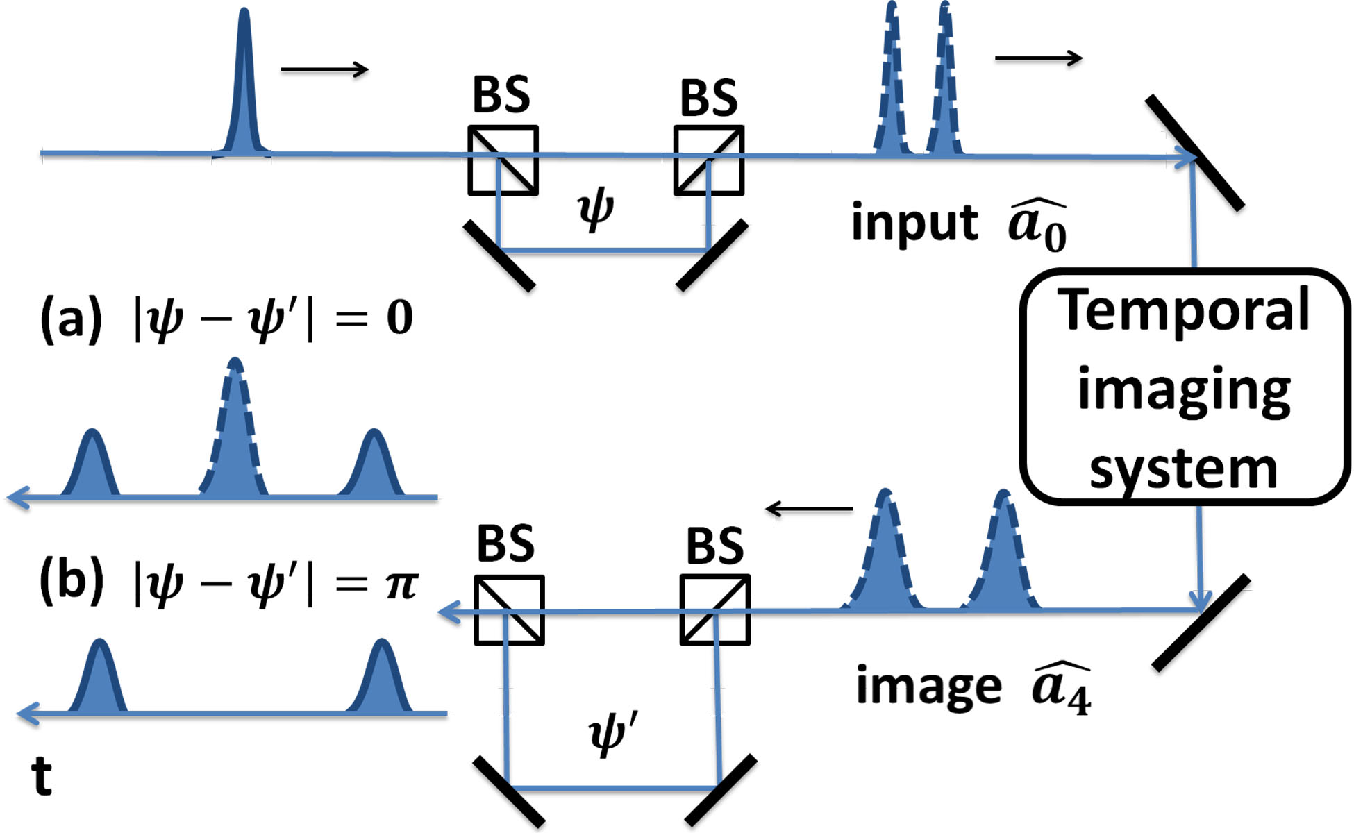
Figure 4: Setup for preparation, temporal imaging and detection of a time-bin entangled photonic wavepacket. Constructive interference (a) and destructive interference (b) in the central peak denote the time-bin entangled state. BS=50/50 beam splitter.

As an example application of a quantum temporal imaging system, we consider a time-bin entangled coherent photon wavepacket, prepared by splitting a coherent faint laser pulse using a Franson interferometer (shown in Fig. 4). The input wavepacket is a coherent state with a double-Gaussian profile given by

$$\hat{a}_{0}(t)=\frac{1}{2}A_{+}(t)\hat{\alpha}(t)+\frac{1}{2}e^{\imath\psi}A_{-}(t)\hat{\alpha}(t)$$ (24)

where

$$\begin{split}A_{\pm}(t)=e^{-2ln{2}((t/\tau\pm d)^{2}},\\ \hat{\alpha}(t)=\exp(\hat{a}^{\dagger}-\hat{a}),\end{split}$$ (25)

is the coherent state operator, $\tau$ is the width of the Gaussian profile (FWHM), $\Delta t=2d\tau$ is the propagation delay in the interferometer, and $\psi$ is the phase difference between the entangled time bins. The total temporal width of the pattern can be defined as $t_{i}=\Delta t+\tau$.

The image waveform of the time-bin entangled photonic wavepacket is given by Eq. (15)

$$\hat{a}_{4}=\frac{1}{2\sqrt{M}}A_{+}(t/M)\hat{\alpha}(t)+\frac{1}{2\sqrt{M}}e^{\imath\psi}A_{-}(t/M)\hat{\alpha}(t).$$ (26)

As shown in Fig. 4, we split and recombine the output image wavepacket through another unbalanced interferometer, where the time difference and phase between the two paths are adjusted to $M\Delta t$ and $\psi^{\prime}$. The output temporal waveform is expected to be a three-peak profile with interference in the central peak. Constructive interference happens when $|\psi-\psi^{\prime}|=0$, while destructive interference happens when $|\psi-\psi^{\prime}|=\pi$. Since interference pattern crucially depends on the phase, a complete true imaging of the phase information encoded in the original time-bin qubit requires that the residual phase is small throughout the image temporal profile.

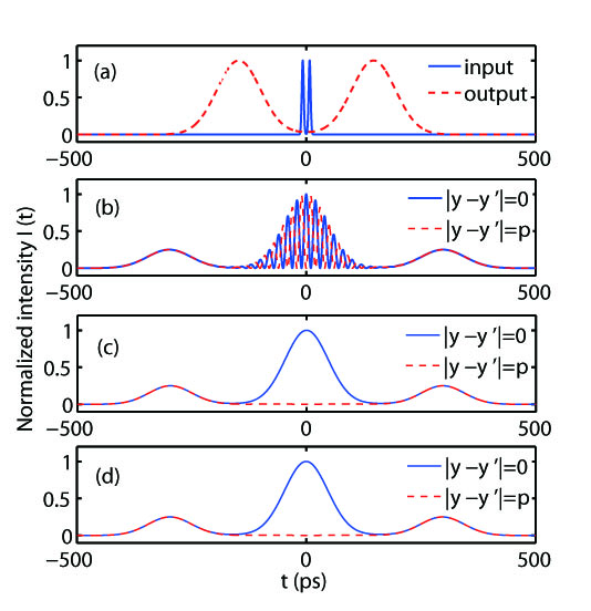
Figure 5: Interference pattern of a temporal imaged time-bin entangled photon wavepacket. (a) Input waveform and perfect image waveform. (b)-(d) Interference pattern after the second interferometer, simulated for the single-lens imaging system (b), telescope system (c) and field lens system (d). Blue solid line shows the constructive interference pattern when $|\psi-\psi^{\prime}|=0$, red dashed line shows the destructive interference pattern when $|\psi-\psi^{\prime}|=\pi$. The visibility $v$ is calculated for the central peak. We obtain $v=0.984$ for field lens and $v=0.986$ for the telescope system, while in the single lens system, fast varying residual phase washes out the visibility.

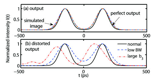
Figure 6: Intensity profile aberrations. (a) Simulated image waveforms using the single-lens imaging system (blue dot-dash), telescope system (green dot) and field lens system (red dash), which are almost identical to each other and closely match the expected perfect output waveform (black solid). (b) Output waveforms in two severe-distorted situations, insufficient bandwidth $\tau_{p}=\tau$ (red dash) and large third-order dispersion $\beta_{3}/\beta_{2}=1$ ps$\sim\tau$ (blue dot-dash), compared to the expected perfect output waveform (black solid).

We numerically simulate the evolution of the waveform using Eq. (11). In the simulation, we set $\tau=5$ ps, $t_{i}=20$ ps, pump pulse initial width $\tau_{p}=0.5\tau$ (pump spectrum is twice as large as the input signal spectrum), and $M=20$, We simulate the image waveform intensity profile $I(t)=\langle\hat{a}(t)a(t)^{\dagger}\rangle$ and the interference pattern for the single-lens system, telescope system, and the field lens system. The largest dispersion in each system is restricted to $Mt_{i}^{2}/8=1,000$ ps². The output intensity profiles are shown in Fig. 5(a) and Fig. 6(a). As shown in the figure, good image waveform profiles are formed regardless of the configuration. Residual phase aberration does not affect the intensity profile of the image waveform, as expected.

The interference results for the time-bin qubit are shown in Fig. 5(b-d). We see that the interference patterns are quite different due to the residual phase. In the single-lens system, the residual phase is large over the temporal profile and washes out the the interference in the central peak (Fig. 5(b), visibility $v=0$). The field lens (Fig. 5(c)) and telescope configuration (Fig. 5(d)) both have successfully removed the residual phase, resulting in a high interference visibility.

We also consider two non-ideal factors that causes possible distortions to the waveform in the simulation: pump-intensity variation and third-order dispersion. The Gaussian profile of the dispersed pump beam pulse has intensity variation, which reduces the conversion efficiency in the side wings of the input photonic wavepacket, hence causing distortion of the imaged waveform. A slight distortion of the waveform towards the center is shown in Fig. 6(a). Such distortion becomes serious when the pump pulse does not have sufficient bandwidth, as shown in Fig. 6(b) for $\tau_{p}=\tau$. The distortion is reduced by increasing the bandwidth of the pump pulse, which flattens the intensity variation.

The dotted-dash line in Fig. 6(b) shows how higher-order dispersion distorts the quadratic nature of the phase modulation and causes aberration in the temporal imaging system, similar to spherical aberration in spatial imaging system. It becomes serious when $\beta_{3}/\beta_{2}>\tau$, and introduces asymmetric distortion to the waveform. In the simulation, we use $\beta_{3}/\beta_{2}=1$ ps$\sim\tau$. This aberration is not apparent when we use a value for third-order dispersion $\beta_{3}/\beta_{2}\sim 0.1$ ps$<<\tau$ that is appropriate for a single-mode fiber SMF-28 at 1550 nm.

V Conclusion

We demonstrate a quantum temporal imaging system that allows us to simultaneously match the wavelengths of two quantum memories and match their characteristic time scales, enabling exchange of quantum information between different quantum platforms such as quantum dots and ions. A field lens in the image plane eliminates the residual phase in the temporal imaging system. When applied to a time-bin entangled photonic wavepacket, the image waveform has good interference visibility, which demonstrates that the field lens configuration is a good candidate for phase-sensitive quantum information applications.

We gratefully acknowledge the financial support of the U.S. Army Research Office MURI award W911NF0910406.

References

- Gisin et al. (2002) N. Gisin, G. Ribordy, W. Tittel, and H. Zbinden, Rev. Mod. Phys. 74, 145 (2002).
- Leibfried et al. (2003) D. Leibfried, R. Blatt, C. Monroe, and D. Wineland, Rev. Mod. Phys. 75, 281 (2003).
- Gisin and Thew (2007) N. Gisin and R. Thew, Nat. Photonics 1, 165 (2007).
- Kimble (2008) H. J. Kimble, Nature (London) 453, 1023 (2008).
- Raymer and Srinivasan (2012) M. G. Raymer and K. Srinivasan, Phys. Today 65, 32 (2012).
- Stute et al. (2013) A. Stute, B. Casabone, B. Brandstätter, K. Friebe, T. Northup, and R. Blatt, Nature Photonics (2013).
- Waks and Monroe (2009) E. Waks and C. Monroe, Phys. Rev. A 80, 062330 (2009).
- Kim et al. (2011) T. Kim, P. Maunz, and J. Kim, Phys. Rev. A 84, 063423 (2011).
- Cirac et al. (1997) J. I. Cirac, P. Zoller, H. J. Kimble, and H. Mabuchi, Phys. Rev. Lett. 78, 3221 (1997).
- Söller et al. (2010) C. Söller, B. Brecht, P. J. Mosley, L. Y. Zang, A. Podlipensky, N. Y. Joly, P. S. J. Russell, and C. Silberhorn, Phys. Rev. A 81, 031801 (2010).
- Kumar (1990) P. Kumar, Opt. Lett. 15, 1476 (1990).
- Huang and Kumar (1992) J. Huang and P. Kumar, Phys. Rev. Lett. 68, 2153 (1992).
- Albota and Wong (2004) M. A. Albota and F. N. C. Wong, Opt. Lett. 29, 1449 (2004).
- Langrock et al. (2005) C. Langrock, E. Diamanti, R. Roussev, Y. Yamamoto, M. Fejer, and H. Takesue, Opt. Lett. 30, 1725 (2005).
- VanDevender and Kwiat (2007) A. P. VanDevender and P. G. Kwiat, JOSA B 24, 295 (2007).
- Pelc et al. (2011) J. S. Pelc, L. Ma, C. R. Phillips, Q. Zhang, C. Langrock, O. Slattery, X. Tang, and M. M. Fejer, Opt. Express 19, 21445 (2011).
- Rakher et al. (2010) M. T. Rakher, L. Ma, O. Slattery, X. Tang, and K. Srinivasan, Nat. Photonics 4, 786 (2010).
- Shahriar et al. (2012) M. Shahriar, P. Kumar, and P. Hemmer, Journal of Physics B: Atomic, Molecular and Optical Physics 45, 124018 (2012).
- Mejling et al. (2012) L. Mejling, C. J. McKinstrie, M. G. Raymer, and K. Rottwitt, Opt. Express 20, 8367 (2012).
- McKinstrie et al. (2005a) C. J. McKinstrie, J. Harvey, S. Radic, and M. G. Raymer, Opt. Express 13, 9131 (2005a).
- McKinstrie et al. (2005b) C. J. McKinstrie, M. Yu, M. G. Raymer, and S. Radic, Opt. Express 13, 4986 (2005b).
- McGuinness et al. (2010) H. J. McGuinness, M. G. Raymer, C. J. McKinstrie, and S. Radic, Phys. Rev. Lett. 105, 93604 (2010).
- Clemmen et al. (2012) S. Clemmen, R. Van Laer, A. Farsi, J. Levy, M. Lipson, and A. Gaeta, in CLEO: QELS-Fundamental Science,OSA Technical Digest (Optical Society of America, 2012) p. QM2H.6.
- Pe’Er et al. (2005) A. Pe’Er, B. Dayan, A. A. Friesem, and Y. Silberberg, Phys. Rev. Lett. 94, 73601 (2005).
- Kielpinski et al. (2011) D. Kielpinski, J. F. Corney, and H. M. Wiseman, Phys. Rev. Lett. 106, 130501 (2011).
- Brecht et al. (2011) B. Brecht, A. Eckstein, A. Christ, H. Suche, and C. Silberhorn, New J. Phys. 13, 065029 (2011).
- McKinstrie et al. (2012) C. J. McKinstrie, L. Mejling, M. G. Raymer, and K. Rottwitt, Phys. Rev. A 85, 053829 (2012).
- Kolner and Nazarathy (1989) B. H. Kolner and M. Nazarathy, Opt. Lett. 14, 630 (1989).
- Tsang and Psaltis (2006) M. Tsang and D. Psaltis, Phys. Rev. A 73, 013822 (2006).
- Salem et al. (2008) R. Salem, M. A. Foster, A. C. Turner, D. F. Geraghty, M. Lipson, and A. L. Gaeta, Opt. Lett. 33, 1047 (2008).
- Foster et al. (2009) M. A. Foster, R. Salem, Y. Okawachi, A. C. Turner-Foster, M. Lipson, and A. L. Gaeta, Nat. Photonics 3, 581 (2009).
- Foster et al. (2008) M. A. Foster, R. Salem, D. F. Geraghty, A. C. Turner-Foster, M. Lipson, and A. L. Gaeta, Nature (Loudon) 456, 81 (2008).
- Loudon (2000) R. Loudon, The quantum theory of light (Third edition, Oxford University Press, 2000) , Chap.6.
- Boyd (2003) R. W. Boyd, Nonliner optics (Second Edition, Academic Pr, 2003) , Chap. 2.
- Born and Wolf (1999) M. Born and E. Wolf, Principle of Optics (Seventh Edition, Cambridge University Press, 1999) , Chap. 5.
- Victor Torres-Company and Weiner (2011) D. E. L. Victor Torres-Company and A. M. Weiner, Opt. Express 19, 24718 (2011).
- Lee et al. (2006) G. H. Lee, S. Xiao, and A. M. Weiner, IEEE Photonics Technol. Lett. 18, 1819 (2006).
- Diebold et al. (2011) E. D. Diebold, N. K. Hon, Z. Tan, J. Chou, T. Sienicki, C. Wang, and B. Jalali, Opt. Express 19, 23809 (2011).
- Loiseaux et al. (1996) B. Loiseaux, A. Delboulbé, J. P. Huignard, P. Tournois, G. Cheriaux, and F. Salin, Opt. Lett. 21, 806 (1996).
- Littler et al. (2005) I. Littler, L. Fu, and B. J. Eggleton, Appl. Opt. 44, 4702 (2005).
- Shverdin et al. (2010) M. Y. Shverdin, F. Albert, S. G. Anderson, S. M. Betts, D. J. Gibson, M. J. Messerly, F. V. Hartemann, C. W. Siders, and C. Barty, Opt. Lett. 35, 2478 (2010).