Mining Representative Unsubstituted Graph Patterns Using Prior Similarity Matrix

Abstract

One of the most powerful techniques to study protein structures is to look for recurrent fragments (also called substructures or spatial motifs), then use them as patterns to characterize the proteins under study. An emergent trend consists in parsing proteins three-dimensional (3D) structures into graphs of amino acids. Hence, the search of recurrent spatial motifs is formulated as a process of frequent subgraph discovery where each subgraph represents a spatial motif. In this scope, several efficient approaches for frequent subgraph discovery have been proposed in the literature. However, the set of discovered frequent subgraphs is too large to be efficiently analyzed and explored in any further process. In this paper, we propose a novel pattern selection approach that shrinks the large number of discovered frequent subgraphs by selecting the representative ones. Existing pattern selection approaches do not exploit the domain knowledge. Yet, in our approach we incorporate the evolutionary information of amino acids defined in the substitution matrices in order to select the representative subgraphs. We show the effectiveness of our approach on a number of real datasets. The results issued from our experiments show that our approach is able to considerably decrease the number of motifs while enhancing their interestingness.

Database Applications - Data Mining]

1 Introduction

Studying protein structures can reveal relevant structural and functional information which may not be derived from protein sequences alone. During recent years, various methods that study protein structures have been elaborated based on diverse types of descriptor such as profiles [25], spatial motifs [17, 21] and others. Yet, the exponential growth of online databases such as the Protein Data Bank (PDB) [4], CATH [7], SCOP [2] and others, arises an urgent need for more accurate methods that will help to better understand the studied phenomenons such as protein evolution, functions, etc.

In this scope, proteins have recently been interpreted as graphs of amino acids and studied based on graph theory concepts [14]. This representation enables the use of graph mining techniques to study protein structures in a graph perspective. In fact, in graph mining, any problem or object under consideration is represented in the form of nodes and edges and studied based on graph theory concepts [3, 12, 16, 6]. One of the powerful and current trends in graph mining is frequent subgraph discovery. It aims to discover subgraphs that frequently occur in a graph dataset and use them as patterns to describe the data. These patterns are lately analyzed by domain experts to reveal interesting information hidden in the original graphs, such as discovering pathways in metabolic networks [9], identifying residues that play the role of hubs in the protein and stabilize its structure [24], etc.

The graph isomorphism test is one of the main bottlenecks of frequent subgraph mining. Yet, many efficient and scalable algorithms have been proposed in the literature and made it feasible for instance FFSM [15], gSpan [29], GASTON [18], etc. Unfortunately, the exponential number of discovered frequent subgraphs is another serious issue that still needs more attention [27], since it may hinder or even make any further analysis unfeasible due to time, resources, and computational limitations. For example, in an AIDS antiviral screen dataset composed of 422 chemical compounds, there are more than 1 million frequent substructures when the minimum support is 5%. This problem becomes even more serious with graphs of higher density such as those representing protein structures. In fact, the issues raised from the huge number of frequent subgraphs are mainly due to two factors, namely redundancy and significance [22]. Redundancy in a frequent subgraph set is caused by structural and/or semantic similarity, since most discovered subgraphs differ slightly in structure and may infer similar or even the same meaning. Moreover, the significance of the discovered frequent subgraphs is only related to frequency. This yields an urgent need for efficient approaches allowing to select relevant patterns among the large set of frequent subgraphs.

In this paper, we propose a novel selection approach which selects a subset of representative patterns from a set of labeled subgraphs, we term them unsubstituted patterns. In order to select these unsubstituted patterns and to shrink the large size of the initial set of frequent subgraphs, we exploit a specific domain knowledge, which is the substitution between amino acids represented as nodes. Though, the main contribution of this work is to define a new approach for mining a representative summary of the set of frequent subgraphs by incorporating a specific background domain knowledge which is the ability of substitution between nodes labels in the graph. In this work, we apply the proposed approach on protein structures because of the availability of substitution matrices in the literature, however, it can be considered as general framework for other applications whenever it is possible to define a matrix quantifying the possible substitution between the labels. Our approach can also be used on any type of subgraph structure such as cliques, trees and paths (sequences). In addition, it can be easily coupled with other pattern selection methods such as discrimination or orthogonality based approaches. Moreover, this approach is unsupervised and can help in various mining tasks, unlike other approaches that are supervised and dedicated to a specific task such as classification.

The remainder of the paper is organized as follows. Section 2 discusses the recent related works in the area of pattern selection for subgraphs. In Section 3, we present the background of our work and we define the preliminary concepts as well as the main algorithm of our approach. Then, Section 4 describes the characteristics of the used data and the experimental settings. Section 5 presents the obtained experimental results and the discussion. It is worth noting that in the rest of the paper, we use the following terms interchangeably : spatial motifs, patterns, subgraphs.

2 Related Works

Recently, several approaches have been proposed for pattern selection in subgraph mining. In [5], authors proposed ORIGAMI, an approach for both subgraph discovery and selection. First they randomly mine a sample of maximal frequent subgraphs, then straightforwardly they select an $\alpha$-orthogonal (non-redundant), $\beta$-representative subgraphs from the mined set. The LEAP algorithm proposed in [28] tries to locate patterns that individually have high discrimination power, using an objective function score that measures each pattern’s significance. Another approach termed gPLS was proposed in [20]. It attempts to select a set of informative subgraphs in order to rapidly build a classifier. gPLS uses the mathematical concept of partial least squares regression to create latent variables allowing a better prediction. COM [16] is another subgraph selection approach which follows a process of pattern mining and classifier learning. It mines co-occurrence rules. Then, based on the co-occurrence information it assembles weak features in order to generate strong ones. In [22], authors proposed a feature selection approach termed CORK. To find frequent subgraphs, it uses the state-of-the-art approach gSpan. Then using a submodular quality function, it selects among them the subset of subgraphs that are most discriminative for classification. In [10], authors designed LPGBCMP, a general model which selects clustered features by considering the structure relationship between subgraph patterns in the functional space. The selected subgraphs are used as weak classifiers (base learners) to obtain high quality classification models. To the best of our knowledge, in all existing subgraph selection approaches [11], the selection is usually based on structural similarity [5] and/or statistical measures (e.g. frequency and coverage (closed [30], maximal [23]), discrimination [22], …). Yet, the prior information and knowledge about the domain are often ignored. However, these prior knowledge may help building dedicated approaches that best fit the studied data.

3 Mining Representative Unsubstituted Patterns

3.1 Background

Statistical pattern selection methods have been widely used to resolve the dimensionality problem when the number of discovered patterns is too large. However, these methods are too generic and do not consider the specificity of the domain and the used data. We believe that in many contexts, it would be important to incorporate the background knowledge about the domain in order to create approaches that best fit the considered data. In proteomics, a protein structure is composed by the folding of a set of amino acids. During evolution, amino acids can substitute each other. The scores of substitution between pairs of amino acids were quantified by biologists in the literature in the form of substitution matrices such as Blosum62 [8]. Our approach uses the substitution information given in the substitution matrices in order to select a subset of unsubstituted patterns that summarizes the whole set of frequent subgraphs. We consider the selected patterns as the representative ones.

The main idea of our approach is based on node substitution. Since the nodes of a protein graph represent amino acids, though, using a substitution matrix, it would be possible to quantify the substitution between two given subgraphs. Starting from this idea, we define a similarity function that measures the distance between a given pair of subgraphs. Then, we preserve only one subgraph from each pair having a similarity score greater or equal to a user specified threshold such that the preserved subgraphs represent the set of representative unsubstituted patterns. An overview of the proposed approach is illustrated in Figure 1 and a more detailed description is given in the following sections.

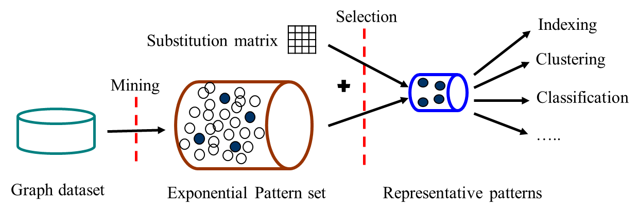
Figure 1: Unsubstituted pattern selection framework.

The substitution between amino acids was also used in the literature but for sequential feature extraction from protein sequences in [19], where the authors proposed a novel feature extraction approach termed DDSM for protein sequence classification. Their approach is restricted to protein sequences and generates every subsequence substituting another one. In other words, DDSM eliminates any pattern substituted by another one and which itself does not substitute any other one. We believe that their approach does not guarantee an optimal summarization since its output may still contain patterns that substitute each other. In addition, they do consider negative substitution scores as impossible substitutions which is biologically not true since negative scores are only expressing the less likely substitutions, which obviously does not mean that they are impossible. Moreover, DDSM is limited to protein sequences and does not handle more complex structures such as the protein tertiary structure. Our approach overcomes these shortcomings, since it can handle both protein sequences and structures (since a sequence can be seen as a line graph). In addition, it consider both the positive and negative scores of the matrix. Moreover, our approach generates a set of representative unsubstituted patterns ensuring an optimal summarization of the initial set. Besides, it is unsupervised and can be exploited in classification as well as other analysis and knowledge discovery contexts unlike DDSM which is dedicated to classification.

3.2 Preliminaries

In this section we present the fundamental definitions and the formal problem statement. Let $\mathcal{G}$ be a dataset of graphs. Each graph $G=(V,E,L)$ of $\mathcal{G}$ is given as a collection of nodes $V$ and a collection of edges $E$. The nodes of $V$ are labeled within an alphabet $L$. We denote by $|V|$ the number of nodes (also called the graph order) and by $|E|$ the number of edges (also called the graph size). Let also $\Omega$ be the set of frequent subgraphs extracted from $\mathcal{G}$, also referred here as $patterns$.

Definition 1.

(Substitution matrix) Given an alphabet $L$, a substitution matrix $\mathcal{M}$ over $L$ is the function defined as:

$$\begin{array}[]{l|rcl}\mathcal{M}:&L^{2}&\longrightarrow&[\bot,\top]\subset\mathds{R}\\ &(l,l^{\prime})&\longmapsto&x\end{array}$$ (1)

The higher the value of $x$ is, the likely is the substitution of $l^{\prime}$ by $l$. If $x=\bot$ then the substitution is impossible, and if $x=\top$ then the substitution is certain. The values $\bot$ and $\top$ are optional and user-specified. They may appear or not in $\mathcal{M}$. The scores in $\mathcal{M}$ should respect the following two properties:

1. $\forall$ l $\in$ L, $\exists$ l’ $\in$ L $\mid$ $\mathcal{M}(l,l^{\prime})$ $\neq$ $\bot$,

2. $\forall$ l $\in$ L, if $\exists$ l’ $\in$ L $\mid$ $\mathcal{M}(l,l^{\prime})$ = $\top$ then $\forall$ l" $\in$ L$\setminus${l, l’}, $\mathcal{M}(l,l")$ = $\bot$ and $\mathcal{M}(l^{\prime},l")$ = $\bot$.

In many real world applications, the substitution matrices may contain at the same time positive and negative scores. In the case of protein’s substitution matrices, both positive and negative values represents possible substitutions. However, positive scores are given to the more likely substitutions while negative scores are given to the less likely substitutions. Though, in order to give more magnitude to higher values of $x$, $\forall$ $l$ and $l^{\prime}$ $\in$ $L$:

$$\mathcal{M}(l,l^{\prime})=\mathrm{e}^{\mathcal{M}(l,l^{\prime})}$$ (2)

Definition 2.

(Structural isomorphism) Two patterns $P=(V_{P},E_{P},L)$ and $P^{\prime}=(V_{P^{\prime}},E_{P^{\prime}},L)$ are said to be structurally isomorphic (having the same shape), we note $shape(P,P^{\prime})$. $shape(P,P^{\prime})=true$ , iff:

1. $P$ and $P^{\prime}$ have the same order, $i.e.,|V_{P}|=|V_{P^{\prime}}|$,

2. $P$ and $P^{\prime}$ have the same size, $i.e.,|E_{P}|=|E_{P^{\prime}}|$,

3. $\exists$ a bijective function $f:V_{P}\rightarrow V_{P^{\prime}}\mid\forall u,v\in V_{P}$ if $(u,v)\in E_{P}$ then $(f(u),f(v))\in E_{P^{\prime}}$ and inversely.

It is worth mentioning that in the graph isomorphism problem we test whether two graphs are exactly the same by considering both structures and labels. But in this definition, we only test whether two given graphs are structurally the same, in terms of nodes and edges, without considering the labels.

Definition 3.

(Elementary mutation probability) Given a node $v$ of a label $l\in L$, the elementary mutation probability, $M_{el}(v)$, measures the possibility that $v$ stay itself and does not mutate to any other node depending on its label $l$.

$$M_{el}(v)=\begin{cases}0,\textit{ if }\mathcal{M}(l,l)=\mathrm{e}^{\bot}\\ 1,\textit{ if }\mathcal{M}(l,l)=\mathrm{e}^{\top}\\ \frac{\mathcal{M}(l,l)}{\sum_{i=1}^{|L|}\mathcal{M}(l,l_{i})},\textit{otherwise}\end{cases}$$ (3)

Obviously, if the substitution score in $\mathcal{M}$ between $l$ and itself is $\bot$ then it is certain that $l$ will mutate to another label $l^{\prime}$ and the probability value that $v$ does not mutate should be 0. Respectively, if this substitution score is $\top$ then it is certain that $v$ will stay itself and conserve its label $l$ so the probability value must be equal to 1. Otherwise, we divide the score that $l$ mutates to itself by the sum of all the possible mutations.

Definition 4.

(Pattern mutation probability) Given a pattern $P=(V_{P},E_{P},L)\in\Omega$, the pattern mutation probability, $M_{patt}(P)$, measures the possibility that $P$ mutates to any other pattern having the same order.

$$M_{patt}(P)=1-\prod_{i=1}^{\mid V_{P}\mid}M_{el}(P[i])$$ (4)

where $\prod_{i=1}^{|V_{P}|}M_{el}(P[i])$ represents the probability that the pattern $P$ does not mutate to any other pattern $i.e.$ $P$ stays itself.

Definition 5.

(Elementary substitution probability) Given two nodes $v$ and $v^{\prime}$ having correspondingly the labels $l,l^{\prime}\in L$, the elementary substitution probability, $S_{el}(v,v^{\prime})$, measures the possibility that $v$ substitutes $v^{\prime}$.

$$S_{el}(v,v^{\prime})=\frac{\mathcal{M}(l,l^{\prime})}{\mathcal{M}(l,l)}$$ (5)

It is worth noting that $S_{el}$ is not bijective $i.e.$ $S_{el}(v,v^{\prime})$ $\neq$ $S_{el}(v^{\prime},v)$.

Definition 6.

(Pattern substitution score) Given two patterns $P=(V_{P},E_{P},L)$ and $P^{\prime}=(V_{P^{\prime}},E_{P^{\prime}},L)$ having the same shape, we denote by $S_{patt}(P,P^{\prime})$ the substitution score of $P^{\prime}$ by $P$. In other words, it measures the possibility that $P$ mutates to $P^{\prime}$ by computing the sum of the elementary substitution probabilities then normalize it by the total number of nodes of $P$. Formally:

$$S_{patt}(P,P^{\prime})=\frac{\sum_{i=1}^{\mid V_{P}\mid}S_{el}(P[i],P^{\prime}[i])}{\mid V_{P}\mid}$$ (6)

Definition 7.

(Pattern substitution) A pattern $P$ substitutes a pattern $P^{\prime}$, we note $subst(P,P^{\prime},\tau)=true$, iff:

1. $P$ and $P^{\prime}$ are structurally isomorphic ($shape(P,P^{\prime})=true$),

2. $S_{patt}(P,P^{\prime})\geq\tau$, where $\tau$ is a user-specified threshold such that $0\%\leq\tau\leq 100\%$.

Definition 8.

(Unsubstituted pattern) Given a threshold $\tau$ and $\Omega^{*}$ $\in\Omega$, a pattern $P^{*}\in\Omega^{*}$ is said to be unsubstituted iff $\nexists P\in\Omega^{*}$ $\mid$ $M_{patt}(P)>M_{patt}(P^{*})$ and $subst(P,P^{*},\tau)=true$.

Proposition 1 (Null $M_{patt}$ case).

Given a pattern $P=(V_{p},E_{p},L)\in\Omega$, if $M_{patt}(P)=0$ then $P$ is an unsubstituted pattern.

Proof.

The proof can be simply deduced from Definitions 3 and 4. ∎

Definition 9.

(Merge support) Given two patterns $P$ and $P^{\prime}$, if $P$ substitutes $P^{\prime}$ then $P$ will represent $P^{\prime}$ in the list of graphs where $P^{\prime}$ occurs. Formally:

$$\forall(P,P^{\prime})\mid subst(P,P^{\prime},\tau)=true\textit{ }then\textit{ }D_{P}=D_{P}\cup D_{P^{\prime}}$$ (7)

where $D_{P}$ and $D_{P^{\prime}}$ are correspondingly the occurrence set of $P$ and that of $P^{\prime}$.

3.3 Algorithm

Given a set of patterns $\Omega$ and a substitution matrix $\mathcal{M}$, we propose UnSubPatt(see Algorithm 1), a pattern selection algorithm which enables detecting the set of unsubstituted patterns $\Omega^{*}$ within $\Omega$. Based on our similarity concept, all the patterns in $\Omega^{*}$ are dissimilar, since it does not contain any pair of patterns that are substitutable. This represents a reliable summarization of $\Omega$.

Data: $\Omega$, $\mathcal{M}$, $\tau$, ($\bot$,$\top$) [Optional]

Result: $\Omega^{*}$: {unsubstituted patterns}

begin

       $\Omega\leftarrow\{\Omega^{k}\leftarrow\{P\in\Omega\textit{ }\mid\textit{ }\forall(P^{\prime},P")\in\Omega^{k},|V_{P^{\prime}}|=|V_{P"}|$ and $|E_{P^{\prime}}|=|E_{P"}|\}\}$;

       foreach $\Omega^{k}\in\Omega$ do

             $\Omega^{k}\leftarrow sort(\Omega^{k}\textit{ }by\textit{ }M_{patt})$;

             foreach $P\in\Omega^{k}$ do

                   if $M_{patt}(P)>0$ then

                         foreach $P^{\prime}\in\Omega^{k}\backslash P$ $|$ $M_{patt}(P^{\prime})<M_{patt}(P)$ do

                               if $M_{patt}(P^{\prime})>0$ then

                                     if $shape(P,P^{\prime})$ and $subst(P,P^{\prime},\tau)$ then

                                           $merge\_support(P,P^{\prime})$;

                                           $remove(P^{\prime},\Omega^{k})$;

                                          

             $\Omega^{*}\leftarrow\Omega^{*}\cup\Omega^{k}$;

            

Algorithm 1 UnSubPatt

The general process of the algorithm is described as follows: first, $\Omega$ is divided into subsets of patterns having the same number of nodes and edges. Then, each subset is sorted in a descending order by the pattern mutation probability $M_{patt}$. Each subset is browsed starting from the pattern having the highest $M_{patt}$. For each pattern, we remove all the patterns it substitutes and we merge their supports such that the preserved pattern will represent all the removed ones wherever they occurs. The remaining patterns represent the unsubstituted pattern set. Though, $\Omega^{*}$ can not be summarized by a subset of it but itself. Our algorithm uses Proposition 1 to avoid unnecessary computation related to patterns with $M_{patt}=0$. They are directly considered as unsubstituted patterns, since they can not mutate to any other pattern.

Theorem 1

Let $\Omega$ be a set of patterns and $\Omega^{*}$ its subset of unsubstituted patterns based on a substitution matrix $\mathcal{M}$ and a threshold $\tau$, $i.e.$, UnSubPatt $(\Omega,\mathcal{M},\tau,(\bot,\top))=\Omega^{*}$. Then :

$$\textsc{UnSubPatt}(\Omega^{*},\mathcal{M},\tau,(\bot,\top))=\Omega^{*}$$ (8)

Proof.

The proof can be deduced simply from Definition 8. Given a threshold $\tau$, $\Omega^{*}$ can not be summarized by its subsets unless itself. Formally:

$$\forall P\in\Omega^{*},\nexists P^{\prime}\in\Omega^{*}|M_{patt}(P)>M_{patt}(P^{\prime})\textit{ }and\textit{ }subst(P,P^{\prime},\tau)$$ (9)

∎

3.4 Complexity

Suppose $\Omega$ contains $n$ patterns. $\Omega$ is divided into $g$ groups, each containing patterns of order $k$. This is done in $O(n)$. Each group $\Omega^{k}$ is sorted in $O(|\Omega^{k}|*log|\Omega^{k}|)$. Searching for unsubstituted patterns requires browsing $\Omega^{k}$ $(O(|\Omega^{k}|))$ and for each pattern, browsing in the worst case all remaining patterns $(O(|\Omega^{k}|))$ to check the shape $(O(k))$ and the substitution $(O(k))$. This means that searching for unsubstituted patterns in a group $\Omega^{k}$ can be done in $O(|\Omega^{k}|^{2}*k^{2})$. Hence, in the worst case, the complexity of our algorithm is $O(g*m_{max}^{2}*k_{max}^{2})$, where $k_{max}$ is the maximum pattern order and $m_{max}$ is the number of patterns of the largest group $\Omega^{k}$.

4 Experiments

4.1 Datasets

In order to experimentally evaluate our approach, we use four graph datasets of protein structures, which also have been used in [28] then [10]. Each dataset consists of two classes: positive and negative. Positive samples are proteins selected from a considered protein family whereas negative samples are proteins randomly gathered from the Protein Data Bank [4]. Each protein is parsed into a graph of amino acids. Each node represents an amino acid residue and is labeled with its amino acid type. Two nodes $u$ and $v$ are linked by an edge $e(u,v)=1$ if the euclidean distance between their two $C_{\alpha}$ atoms $\Delta(C_{\alpha}(u),C_{\alpha}(v))$ is below a threshold distance $\delta$. Formally:

$$e(u,v)=\begin{cases}1,\emph{ }if\emph{ }\Delta(C_{\alpha}(u),C_{\alpha}(v))\leq\delta\\ 0,\emph{ }otherwise\end{cases}$$ (10)

In the literature, many methods use this definition with usually $\delta\geq 7$Å on the argument that $C_{\alpha}$ atoms define the overall shape of the protein conformation [13]. In our experiments, we use $\delta=7$Å.

Table 1 summarizes the characteristics of each dataset. SCOP ID, Avg.$\mid$V$\mid$, Avg.$\mid$E$\mid$, Max.$\mid$V$\mid$ and Max.$\mid$E$\mid$ correspond respectively to the id of the protein family in SCOP database [2], the average number of nodes, the average number of edges, the maximal number of nodes and the maximal number of edges in each dataset.

Table 1: Experimental data

Dataset	SCOP ID	Family name	Pos.	Neg.	Avg.$\mid$V$\mid$	Avg.$\mid$E$\mid$	Max.$\mid$V$\mid$	Max.$\mid$E$\mid$
DS1	52592	G proteins	33	33	246	971	897	3 544
DS2	48942	C1 set domains	38	38	238	928	768	2 962
DS3	56437	C-type lectin domains	38	38	185	719	755	3 016
DS4	88854	Kinases, catalytic subunit	41	41	275	1077	775	3 016

4.2 Protocol and Settings

Generally, in a pattern selection approach two aspects are emphasized, namely the number of selected patterns and their interestingness. In order to evaluate our approach, we first use the state-of-the-art method of frequent subgraph discovery gSpan [29] to find the frequent subgraphs in each dataset with a minimum frequency threshold of 30%. Then, we use UnSubPatt to select the unsubstituted patterns among them with a minimum substitution threshold $\tau$=30%. For our approach, we use $Blosum62$ [8] as the substitution matrix since it turns out that it performs well on detecting the majority of weak protein similarities, and it is used as the default matrix by most biological applications such as BLAST [1]. It is worth mentioning that the choice of 30% as minimum frequency threshold for the frequent subgraph extraction is to make the experimental evaluation feasible due to time and computational limitations.

In order to evaluate the number of selected subgraphs, we define the selection rate as the rate of the number of unsubstituted subgraphs from the initial set of frequent subgraphs. Formally :

$$Selection\textit{ }rate=\frac{|\Omega^{*}|\ast 100}{|\Omega|}$$ (11)

To evaluate the interestingness of the set of selected patterns, we use them as features for classification. We perform a 5-fold cross-validation classification (5 runs) on each protein-structure dataset. We encode each protein into a binary vector, denoting by "1" or "0" the presence or the absence of the feature in the considered protein. To judge the interestingness of the selected subgraphs, we use one of the most known classifier, namely the naïve bayes (NB) classifier, due to its simplicity and fast prediction and that its classification technique is based on a global and conditional evaluation of the input features. NB is used with the default parameters from the workbench Weka [26].

5 Results and Discussion

In this section, we conduct experiments to examine the effectiveness and efficiency of UnSubPatt in finding the representative unsubstituted subgraphs. We test the effect of changing the substitution matrix and the substitution threshold on the results. Moreover, we study the size-based distribution of patterns and we compare the results of our approach with those of other subgraph selection methods from the literature.

5.1 Empirical Results

Here, we show the results of our experiments obtained in terms of number of motifs and classification results. As mentioned before, we use gSpan to extract the frequent subgraphs from each dataset with frequency $\geq$ 30%. Then, we use UnSubPatt to select the unsubstituted patterns among them with a substitution threshold $\tau$=30% and using Blosum62 as substitution matrix. At last, we perform a 5-fold cross-validation classification (5 runs) to evaluate the interestingness of each subset using the NB classifier. The obtained average results are reported in Table 3.

Table 2: Number of frequent subgraphs ($\Omega$), representative unsubstituted subgraphs ($\Omega^{*}$) and the selection rate

Dataset	$\mid\Omega\mid$	$\mid\Omega^{*}\mid$	Selection rate (%)
DS1	799094	7291	0.91
DS2	258371	15898	6.15
DS3	114792	14713	12.82
DS4	1073393	9958	0.93

The high number of discovered frequent subgraphs is due to their combinatorial nature (this was discussed in the introductory section). The results reported in Table 2 show that our approach decreases considerably the number of subgraphs. The selection rate shows that the number of unsubstituted patterns $\mid\Omega^{*}\mid$ does not exceed 13% of the initial set of frequent subgraphs $\mid\Omega\mid$ with DS3 and even reaches less than 1% with DS1 and DS4. This proves that exploiting the domain knowledge, which in this case consists in the substitution matrix, enables emphasizing information that can possibly be ignored when using exiting subgraph selection approaches.

Table 3: Accuracy, precision, recall (sensitivity), F-score and AUC of the classification of each dataset using NB coupled with frequent subgraphs (FSg) then representative unsubstituted subgraphs (UnSubPatt)

Dataset	Accuracy		Precision		Recall		F-score		AUC
	FSg	UnSubPatt	FSg	UnSubPatt	FSg	UnSubPatt	FSg	UnSubPatt	FSg	UnSubPatt
DS1	0.62	0.78	0.61	0.69	0.70	0.90	0.64	0.78	0.64	0.78
DS2	0.80	0.90	0.86	0.94	0.74	0.86	0.79	0.89	0.79	0.89
DS3	0.86	0.94	0.89	1.00	0.86	0.89	0.86	0.94	0.86	0.94
DS4	0.79	0.98	0.86	0.92	0.70	0.98	0.76	0.94	0.76	0.94

The classification results reported in Table 3 help to evaluate the interestingness of the selected patterns. Indeed, this will demonstrate if the unsubstituted patterns were arbitrarily selected or they are really representative. Table 3 shows that the classification accuracy significantly increases with all datasets. We notice a huge leap in accuracy especially with DS1 and DS4 with a gain of more than 17% and reaching almost full accuracy with DS4. To better understand the accuracy results, we also reports the average precision, recall, F-measure and AUC values for all cases. We notice an enhancement of performance with all the mentioned quality metrics. This supports the reliability of our selection approach.

5.2 Results Using Other Substitution Matrices

Besides Blosum62, biologists also defined other substitution matrices describing the likelihood that two amino acid types would mutate to each other in evolutionary time. We want to study the effect of using other substitution matrices on the experimental results. Though, we perform the same experiments following the same protocol and settings but using two other substitution matrices, namely $Blosum80$ and $Pam250$. We compare the obtained results in terms of number of subgraphs and classification accuracy with those obtained using the whole set of frequent subgraphs and those using subgraphs selected by UnSubPatt with Blosum62. The results are reported in Table 4. A high selection rate accompanied with a clear enhancement of the classification accuracy is noticed using UnSubPatt with all the substitution matrices compared to the results using the whole set of frequent subgraphs. It is clearly noticed that even using different substitution matrices, UnSubPatt shows relatively similar behavior and is able to select a small yet relevant subset of patterns. It is also worth mentioning that for all the datasets, the best classification accuracy is obtained using Blosum62 and the best selection rate is achieved using Pam250. This is simply due to how distant proteins within the same dataset are, since each substitution matrix was constructed to implicitly express a particular theory of evolution. Though, choosing the appropriate substitution matrix can influence the outcome of the analysis.

Table 4: Number of subgraphs (#SG) and accuracy (ACC) of the classification of each dataset using NB coupled with frequent subgraphs (FSg) then representative unsubstituted subgraphs using Blosum80 (UnSubPatt_Blosum80) and Pam250 (UnSubPatt_Pam250)

Dataset	FSg		UnSubPatt_Blosum62		UnSubPatt_Blosum80		UnSubPatt_Pam250
	#SG	Accuracy	#SG	Accuracy	#SG	Accuracy	#SG	Accuracy
DS1	799094	0.62	7291	0.78	7328	0.67	6137	0.68
DS2	258371	0.80	15898	0.90	15930	0.87	15293	0.87
DS3	114793	0.86	14713	0.94	14792	0.91	14363	0.93
DS4	1073393	0.79	9958	0.98	10417	0.90	9148	0.90

5.3 Impact of Substitution Threshold

In our experiments, we used a substitution threshold (of 30%) to select the unsubstituted patterns from the set of discovered frequent subgraphs. In this section, we study the impact of variation of the substitution threshold on both the number of selected subgraphs and the classification results. To do so, we perform the same experiments while varying the substitution threshold from 0% to 90% with a step-size of 10. In order to check if the enhancements of the obtained results are due to our selected features or to the classifier, we use two other well-known classifiers namely the support vector machine (SVM) and decision tree (C4.5) besides the naïve bayes (NB) classifier. We use the same protocol and settings of the previous experiments. Figure 2 presents the selection rate for different substitution thresholds and Figures 3, 4 and 5 illustrate the classification accuracy obtained respectively using NB, SVM and C4.5 with each dataset. The classification accuracy of the initial set of frequent subgraphs (gSpan, the line in red) is considered as a standard value for comparison. Thus, the accuracy values of UnSubPatt (in blue) that are above the line of the standard value are considered as gains, and those under the standard value are considered as losses.

In Figure 2, we notice that UnSubPatt reduces considerably the number of subgraphs especially with lower substitution thresholds. In fact, the number of unsubstituted patterns does not exceed 30% for all substitution thresholds below 70% and even reaches less then 1% in some cases. This important reduction in the number of patterns comes with a notable enhancement of the classification accuracies. This fact is illustrated in Figures 3, 4 and 5 which show that the unsubstituted patterns allow better classification performance compared to the original set of frequent subgraphs. UnSubPatt scores very well with the three used classifiers and even reaches full accuracy in some cases. This confirms our assumptions and shows that our selection is reliable and contributes to the enhancement of the accuracy. However, we believe that NB allows the most reliable evaluation because it performs a classification based on a global and conditional evaluation of features, unlike SVM which performs itself another attribute selection to select the support vectors and unlike C4.5 which performs an attribute by attribute evaluation.

In the case of proteins, a substitution threshold of 0% enables selecting subgraphs based only on their structure. Precisely, UnSubPatt will select only one pattern from each group of subgraphs that are structurally isomorphic. Based on the experimental results, we believe that using these patterns is enough for a structural classification task since it allows a fast selection, selects a very small number of subgraphs and performs very well on classification.

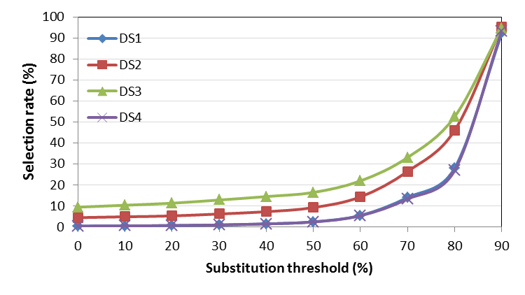
Figure 2: Rate of unsubstituted patterns from $\Omega$ depending on the substitution threshold ($\tau$).

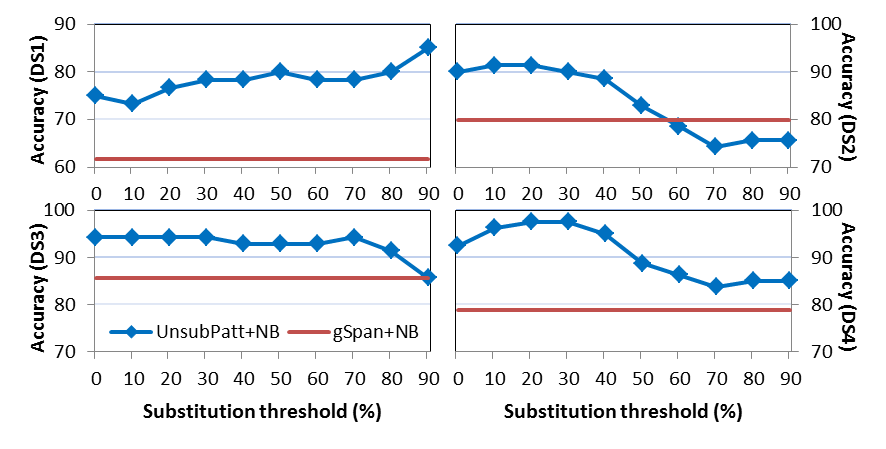
Figure 3: Classification accuracy by NB.

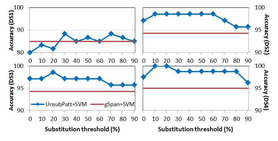
Figure 4: Classification accuracy by SVM.

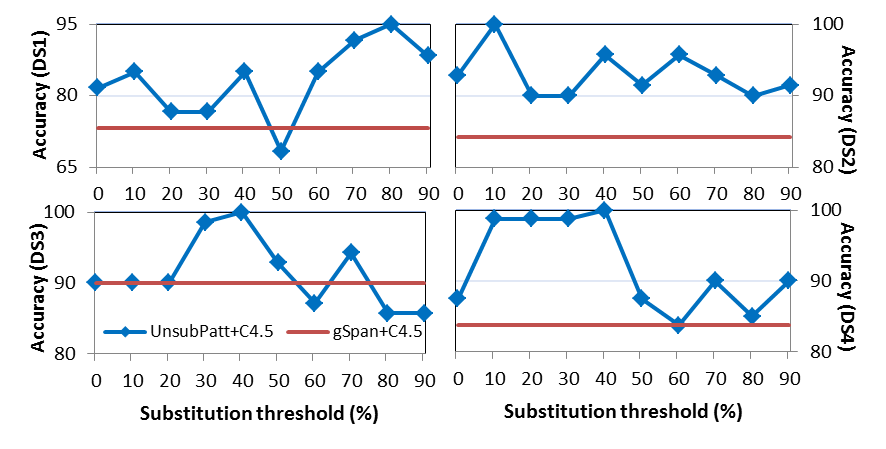
Figure 5: Classification accuracy by C4.5.

5.4 Size-based Distribution of Patterns

In this section, we study the distribution of patterns based on their size (number of edges). We try to check which sizes of patterns are more concerned by the selection. The Figures 6 and 7 draw the distribution of patterns for the original set of frequent subgraphs and for the final set of representative unsubstituted subgraphs with all the substitution thresholds using Blosum62. The downward tendency of UnSubPatt using lower substitution thresholds and with respect to the original set of frequent subgraph is very clear. In fact, UnSubPatt leans towards cutting off the peaks and flattening the curves with lower substitution thresholds. Another interesting observation is that the curves are flattened in the regions of small patterns as well as in those of big and dense patterns. This demonstrates the effectiveness of UnSubPatt with both small and big patterns.

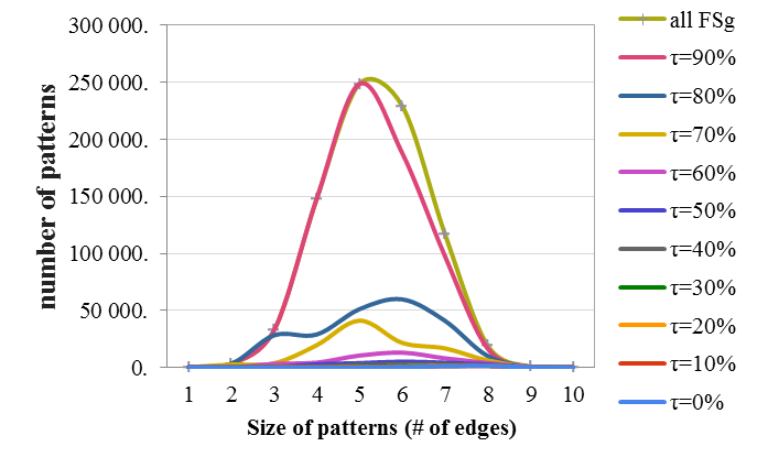
Figure 6: Distribution of patterns of DS1 for all the frequent subgraphs and for the representative unsubstituted ones with all the substitution thresholds

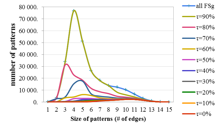
Figure 7: Distribution of patterns of DS2 for all the frequent subgraphs and for the representative unsubstituted ones with all the substitution thresholds

5.5 Comparison with other approaches

To objectively evaluate our approach, we compare it with current trends in subgraph selection. In Figure 8, we report the classification accuracy using the representative unsubstituted patterns of UnSubPatt besides those using patterns of other new subgraph selection approaches from the literature namely LEAP[28], gPLS[20], COM[16] and LPGBCMP[10] (reported and explained in the introductory section).

For UnSubPatt, we report the results obtained using the substitution matrix Blosum62, a minimum substitution threshold $\tau=30\%$ and SVM for classification. For LEAP+SVM, LEAP is used iteratively to discover a set of discriminative subgraphs with a leap length=0.1. The discovered subgraphs are consider as features to train SVM with a 5-fold cross validation. COM is used with $t_{p}=30\%$ and $t_{n}=0\%$. For gPLS, the frequency threshold is set to 30% and the best accuracies are reported for all the datasets among all the parameters combinations from m = 2, 4, 8, 16 and k = 2, 4, 8, 16, where m is the number of iterations and k is the number of patterns obtained per search. For LPGBCMP, threshold values of $max_{v}ar=1$ and $\delta=0.25$ were respectively used for feature consistency map building and for overlapping. The obtained results are reported in the Figure 8.

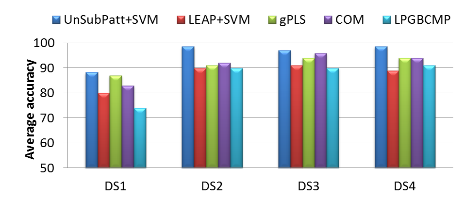
Figure 8: Classification accuracy comparison with other pattern selection approaches.

The classification results displayed in Figure 8 show that UnSubPatt allows a better classification than all the other pattern selection methods in the four cases. Considering only these results does not allow to confirm that UnSubPatt would always outperform the considered methods. However, this proves that UnSubPatt represents a very competitive and promising approach. It is also worth noting that these approaches are supervised and dedicated to classification unlike UnSubPatt which is an unsupervised approach. This allows it to be used in classification as well as in other mining tasks such as clustering and indexing.

5.6 Runtime Analysis

To study the variation of UnSubPatt’s runtime with larger amounts of data, we use different sets of frequent patterns from 10000 to 100000 with step-size of 10000. In Table 5, we report the runtime results for the pattern sets using three substitution thresholds.

Table 5: Runtime analysis of UnSubPatt with different substitution thresholds

Number of	Substitution thresholds
patterns	$\tau$ = 10%	$\tau$ = 30%	$\tau$ = 50%
10000	4s	4s	4s
20000	8s	8s	10s
30000	13s	13s	17s
40000	18s	18s	25s
50000	23s	23s	33s
60000	28s	28s	41s
70000	35s	35s	52s
80000	40s	42s	66s
90000	46s	49s	80s
100000	53s	57s	136s

Even though the complexity of the problem due to the combinatorial test of substitution between subgraphs, our algorithm is scalable with higher amounts of data. With increasing number of patterns, the runtime is still reasonable. The use of different substitution thresholds slightly affected the runtime of UnSubPatt, since the number of selected patterns is comparable for all thresholds.

A possible way to make UnSubPatt runs faster is parallelization. In fact, UnSubPatt can be easily parallelized, since it tests separately the substitution among each group of subgraphs having the same size and order. Hence, these groups can be distributed and treated separately in different processes.

6 Conclusion

In this paper, we proposed a novel selection approach for mining a representative summary of the set of frequent subgraphs. Unlike existent methods that are based on the relations between patterns in the transaction space, our approach considers the distance between patterns in the pattern space. The proposed approach exploits a specific domain knowledge, in the form of a substitution matrix, to select a subset of representative unsubstituted patterns from a given set of frequent subgraphs. It also allows to reduce considerably the size of the initial set of subgraphs to obtain an interesting and representative one enabling easier and more efficient further explorations. It is also worth mentioning that our approach can be used on graphs as well as on sequences and is not limited to classification tasks, but can help in other subgraph-based analysis such as indexing, clustering, visual inspection, etc.

Since the proposed approach is a filter approach, a promising future direction could be to find a way to integrate the selection within the extraction process in order to directly mine the representative patterns from data. Moreover, we intend to use our approach in other classification contexts and in other mining applications.

7 Acknowledgement

This work is supported by a PhD grant from the French Ministry of Higher Education to the first author.

References

- [1] S. Altschul, W. Gish, W. Miller, E. Myers, and D. Lipman. Basic local alignment search tool. Journal of Molecular Biology, 215:403–410, 1990.
- [2] A. Andreeva, D. Howorth, J.-M. Chandonia, S. E. Brenner, T. J. P. Hubbard, C. Chothia, and A. G. Murzin. Data growth and its impact on the scop database: new developments. Nucleic Acids Research, 36(1):D419–D425, 2008.
- [3] L. Bartoli, P. Fariselli, and R. Casadio. The effect of backbone on the small-world properties of protein contact maps. Physical Biology, 4(4):L1+, 2007.
- [4] H. M. Berman, J. D. Westbrook, Z. Feng, G. Gilliland, T. N. Bhat, H. Weissig, I. N. Shindyalov, and P. E. Bourne. The protein data bank. Nucleic Acids Research, 28(1):235–242, 2000.
- [5] V. Chaoji, M. A. Hasan, S. Salem, J. Besson, and M. J. Zaki. Origami: A novel and effective approach for mining representative orthogonal graph patterns. Statistical Analysis and Data Mining, 1(2):67–84, 2008.
- [6] H. Cheng, X. Yan, and J. Han. Mining graph patterns. In Managing and Mining Graph Data, pages 365–392. Springer, 2010.
- [7] A. L. Cuff, I. Sillitoe, T. Lewis, A. B. Clegg, R. Rentzsch, N. Furnham, M. Pellegrini-Calace, D. T. Jones, J. M. Thornton, and C. A. Orengo. Extending cath: increasing coverage of the protein structure universe and linking structure with function. Nucleic Acids Research, 39:420–426, 2011.
- [8] S. R. Eddy. Where did the blosum62 alignment score matrix come from? Nature Biotechnology, pages 1035–1036, 2004.
- [9] K. Faust, P. Dupont, J. Callut, and J. van Helden. Pathway discovery in metabolic networks by subgraph extraction. Bioinformatics, 26(9):1211–1218, 2010.
- [10] H. Fei and J. Huan. Boosting with structure information in the functional space: an application to graph classification. In ACM knowledge discovery and data mining conference (KDD), pages 643–652, 2010.
- [11] M. A. Hasan. Pattern summarization in pattern mining. Encyclopedia of Data Warehousing and Mining, (2nd Ed), 2008.
- [12] M. A. Hasan and M. J. Zaki. Output space sampling for graph patterns. PVLDB, 2(1):730–741, 2009.
- [13] J. Huan, D. Bandyopadhyay, W. Wang, J. Snoeyink, J. Prins, and A. Tropsha. Comparing graph representations of protein structure for mining family-specific residue-based packing motifs. Journal of Computational Biology, 12(6):657–671, 2005.
- [14] J. Huan, W. Wang, D. B, J. Snoeyink, J. Prins, and A. Tropsha. Mining spatial motifs from protein structure graphs. In International Conference on Research in Computational Molecular Biology (RECOMB), pages 308–315, 2004.
- [15] J. Huan, W. Wang, and J. Prins. Efficient mining of frequent subgraphs in the presence of isomorphism. In IEEE International Conference on Data Mining (ICDM), pages 549–552, 2003.
- [16] N. Jin, C. Young, and W. Wang. Graph classification based on pattern co-occurrence. In ACM International Conference on Information and Knowledge Management, pages 573–582, 2009.
- [17] G. J. Kleywegt. Recognition of spatial motifs in protein structures. Journal of molecular biology, 285(4):1887–1897, 1999.
- [18] S. Nijssen and J. N. Kok. A quickstart in frequent structure mining can make a difference. In ACM knowledge discovery and data mining conference (KDD), pages 647–652, 2004.
- [19] R. Saidi, M. Maddouri, and E. Mephu Nguifo. Protein sequences classification by means of feature extraction with substitution matrices. BMC Bioinformatics, 11(1):175+, 2010.
- [20] H. Saigo, N. Krämer, and K. Tsuda. Partial least squares regression for graph mining. In ACM knowledge discovery and data mining conference (KDD), pages 578–586, 2008.
- [21] H. Sun, A. Sacan, H. Ferhatosmanoglu, and Y. Wang. Smolign: A spatial motifs-based protein multiple structural alignment method. IEEE/ACM Transactions on Computational Biology and Bioinformatics, 9(1):249–261, 2012.
- [22] M. Thoma, H. Cheng, A. Gretton, J. Han, H.-P. Kriegel, A. Smola, L. Song, P. S. Yu, X. Yan, and K. M. Borgwardt. Discriminative frequent subgraph mining with optimality guarantees. Statistical Analysis and Data Mining, 3(5):302–318, 2010.
- [23] L. T. Thomas, S. R. Valluri, and K. Karlapalem. Margin: Maximal frequent subgraph mining. ACM Transactions on Knowledge Discovery from Data (TKDD), 4(3):10:1–10:42, 2010.
- [24] R. R. Vallabhajosyula, D. Chakravarti, S. Lutfeali, A. Ray, and A. Raval. Identifying hubs in protein interaction networks. PLoS ONE, 4(4):e5344, 2009.
- [25] N. von Öhsen, I. Sommer, R. Zimmer, and T. Lengauer. Arby: automatic protein structure prediction using profile-profile alignment and confidence measures. Bioinformatics, 20(14):2228–2235, 2004.
- [26] I. H. Witten and E. Frank. Data Mining: Practical Machine Learning Tools and Techniques. Morgan Kaufmann, 2005.
- [27] A. Woznica, P. Nguyen, and A. Kalousis. Model mining for robust feature selection. In ACM knowledge discovery and data mining conference (KDD), pages 913–921, 2012.
- [28] X. Yan, H. Cheng, J. Han, and P. S. Yu. Mining significant graph patterns by leap search. ACM SIGMOD international conference on Management of data, pages 433–444, 2008.
- [29] X. Yan and J. Han. gspan: Graph-based substructure pattern mining. Order A Journal On The Theory Of Ordered Sets And Its Applications, 02:721–724, 2002.
- [30] X. Yan and J. Han. Closegraph: mining closed frequent graph patterns. In ACM knowledge discovery and data mining conference (KDD), pages 286–295, 2003.