Star-forming regions of the Aquila rift cloud complex.

Abstract

Aims. The physics of star formation is an important issue of Galactic evolution. Most stars are formed in high density environments ($n>10^{4}$ cm^-3) emitting lines of diverse molecular transitions. In the present part of our survey we search for ammonia emitters in the Aquila rift complex which trace the densest regions of molecular clouds.

Methods. From a CO survey carried out with the Delingha 14-m telescope we selected $\sim 150$ targets for observations in other molecular lines. Here we describe the mapping observations in the NH₃(1,1) and (2,2) inversion lines of the first 49 sources performed with the Effelsberg 100-m telescope.

Results. The NH₃(1,1) and (2,2) emission lines are detected in 12 and 7 sources, respectively. Among the newly discovered NH₃ sources, our sample includes the following well-known clouds: the starless core L694-2, the Serpens cloud Cluster B, the Serpens dark cloud L572, the filamentary dark cloud L673, the isolated protostellar source B335, and the complex star-forming region Serpens South. Angular sizes between $40^{\prime\prime}$ and $80^{\prime\prime}$ ($\sim 0.04-0.08$ pc) are observed for compact starless cores but as large as $9^{\prime}$ ($\sim 0.5$ pc) for filamentary dark clouds. The measured kinetic temperatures of the clouds lie between 9 K and 18 K. From NH₃ excitation temperatures of $3-8$ K we determine H₂ densities with typical values of $\sim(0.4-4)\times 10^{4}$ cm^-3. The masses of the mapped cores range between $\sim 0.05$ and $\sim 0.5M_{\odot}$. The relative ammonia abundance, $X=$ [NH₃]/[H₂], varies from $1\times 10^{-7}$ to $5\times 10^{-7}$ with the mean $\langle X\rangle=(2.7\pm 0.6)\times 10^{-7}$ (estimated from spatially resolved cores assuming the filling factor $\eta=1$). In two clouds, we observe kinematically split NH₃ profiles separated by $\sim 1$ km s^-1. The splitting is most likely due to bipolar molecular outflows for one of which we determine an acceleration of $\dot{V}\;\raise 1.29167pt\hbox{$<$\kern-7.5pt\raise-4.73611pt\hbox{$\sim$}}\;0.03$ km s^-1 yr^-1. A starless core with significant rotational energy is found to have a higher kinetic temperature than the other ones which is probably caused by magnetic energy dissipation.

1 Introduction

One of the central questions of stellar evolution is about the processes defining the initial mass of a protostellar object. It is suggested that more than 70% of stars are formed in clusters embedded within giant molecular clouds (Lada & Lada 2003) and that the varying environment may affect the initial mass function (IMF).

In the present survey we search for the star-formation regions in the Aquila giant molecular cloud. Starting from Cygnus, in the direction of the Galactic center, the Milky Way appears to be split into two branches. The southern branch runs through Cygnus, Vulpecula, Sagitta, Aquila, and Scutum, entering the Galactic central bulge in Sagittarius. The northern branch crosses Vulpecula and Aquila and disappears in the northern part of the Serpens Cauda and Ophiuchus constellations. The separating dark band of obscuring dust is commonly called the Aquila rift, but absorbing clouds are found not only next to the Galactic plane: many dark clouds are located in areas extending up to latitudes of at least +10^∘ and down to $-20^{\circ}$ (e.g., Dame & Thaddeus 1985; Kawamura et al. 1999; Dobashi et al. 2005).

The distance to the Aquila rift was estimated from optical data and interstellar extinction, and from parallax measurements. A sudden appearance of reddened stars is observed at $D=225\pm 55$ pc and the cloud distribution may have a thickness of $\sim 80$ pc (Strai$\check{\rm z}$ys et al. 2003). This estimate is in line with the distance to the Serpens-Aquila region found from interstellar extinction by Knude (2011), $D=203\pm 7$ pc, but significantly smaller than the trigonometric parallax value $415\pm 25$ pc deduced by Dzib et al. (2010) from the Very Long Baseline Array observations of the young stellar object EC 95 in the Serpens cloud. Since the discrepancy in the distance estimations may be caused by a projection effect, we will use hereafter the weighted harmonic mean of the first two measurements, both based on large-size data sets, $D=203\pm 12$ pc, if not otherwise specified. Thus, comparing to other close molecular complexes, the distance to the Aquila rift is similar to that of the Perseus clouds ($\sim 250$ pc; Rosolowsky et al. 2008) and lies between those of the Taurus and the Pipe Nebula ($\sim 140$ pc; Rathborne et al. 2008) and the Auriga ($\sim 300$ pc) molecular clouds (Heiderman et al. 2010; Cieza et al. 2012).

Recently the Herschel Gould Belt Survey reveals in the Aquila rift cloud complex a large number ($\;\raise 1.29167pt\hbox{$>$\kern-7.5pt\raise-4.73611pt\hbox{$\sim$}}\;500$) of starless cores (e.g., Bontemps et al. 2010; Könyves et al. 2010; Men’shchikov et al. 2010). Starting our investigations of the Aquila clouds we have carried out in 2010 an extended survey of CO and extinction peaks using the Delingha 14-m telescope (Zuo et al. 2004). The targets were selected from the CO data of Kawamura et al. (1999, 2001) and from the optical data of Dobashi et al. (2005), limited in the latter case by the areas with $A_{v}>6^{\rm m}$. We observed and detected 23 Kawamura and 47 Dobashi clouds at $\lambda\sim 3$ mm. However, CO and ¹³CO trace not only the dense gas but also outflows and low density regions; in addition, CO may be saturation broadened. It is well known that the carbon-chain molecules disappear from the gas-phase in the central regions because of freeze-out onto dust grains (e.g., Tafalla et al. 2004), i.e., C-bearing molecules are usually distributed in the outer parts of the cores. That is why CO and ¹³CO are not good indicators for the dense molecular gas. Contrary to this, N-bearing molecules such as ammonia concentrate in the inner cores, where the gas density approaches $10^{5}$ cm^-3. Ammonia is still observable in the gas-phase since it is resistant to depletion onto dust grains (e.g., Bergin & Langer 1997).

Based on the CO survey we composed a list of $\sim 150$ targets where not only CO but also ¹³CO is quite strong, thus indicating large column densities and hence promising conditions to detect dense cores. The objective of the current work performed with the Effelsberg 100-m telescope is to observe these targets in other molecular lines, in the first place in NH₃, in order to confirm the target identifications as dense cores and to determine their physical properties.

In the present paper we describe the first 49 sources from our survey. Observations are described in Sect. 2. Individual molecular cores are considered in Sect. 3. The results obtained are summarized in Sect. 4, and computational methods are outlined in Appendix A. Appendix B contains NH₃(1,1) and (2,2) spectra detected toward the ammonia peaks, tables with derived physical parameters, and maps showing distributions of these parameters within the three most prominent cores.

2 Observations

The ammonia observations were carried out with the Effelsberg 100-m telescope in 4 observing sessions between March 26 and 30, 2011, and in 2 sessions on January 12 and 13, 2012. The NH₃ lines were measured with a K-band HEMT (high electron mobility transistor) dual channel receiver, yielding spectra with full width to half power (FWHP) resolution of $40^{\prime\prime}$ in two orthogonally oriented linear polarizations at the rest frequency of the $(J,K)=(1,1)$ and (2,2) lines (23694.496 MHz and 23722.631 MHz, respectively). Averaging the emission from both channels, the typical system temperature (receiver noise and atmosphere) is 100 K on a main beam brightness temperature scale.

In 2011, the measurements were obtained in frequency switching mode using a frequency throw of $\pm 2.5$ MHz. The backend was an FFTS (fast Fourier transform spectrometer), operated with a bandwidth of 100 MHz, providing simultaneously 16 384 channels for each polarization. For some offsets we also used the minimum bandwidth of 20 MHz for the NH₃(1,1) line. The resulting channel widths were 0.077 km s^-1 and 0.015 km s^-1, respectively. We note, however, that the true velocity resolution was about 1.6 times as large.

In 2012, the measurements were obtained with the backend XFFTS (eXtended bandwidth FFTS), operated with 100 MHz and 2 GHz bandwidths, providing 32 768 channels for each polarization. The resulting channel widths were 0.038 km s^-1 and 0.772 km s^-1, respectively, but the true velocity resolution is 1.16 times larger (Klein et al. 2012).

The pointing was checked every hour by continuum cross scans of nearby continuum sources. The pointing accuracy was better than $5^{\prime\prime}$. The spectral line data were calibrated by means of continuum sources with known flux density. We mainly used NGC7027 (Ott et al. 1994), 3C123 (Baars et al. 1977), and G29.96–0.02 (Churchwell et al. 1990). These calibration sources were used to establish a main beam brightness temperature scale, $T_{\scriptscriptstyle\rm MB}$. Since the main beam size ($40^{\prime\prime}$) is smaller than most core radii ($>50^{\prime\prime}$) of our Aquila objects, the ammonia emission couples well to the main beam and, thus, the $T_{\scriptscriptstyle\rm MB}$ scale is appropriate. Compensations for differences in elevation between the calibrator and the source were $\;\raise 1.29167pt\hbox{$<$\kern-7.5pt\raise-4.73611pt\hbox{$\sim$}}\;20$% and have not been taken into account. Similar uncertainties of the main beam brightness temperature were found from comparison of spectra toward the same position taken at different dates.

3 Results

The detected NH₃ spectra were treated in the way described in Appendix A. We note that the radial velocity, $V_{\scriptscriptstyle\rm LSR}$, the linewidth $\Delta v$ (FWHM), the optical depths, $\tau_{11}$ and $\tau_{22}$, the integrated ammonia emission, $\int$$T_{\scriptscriptstyle\rm MB}$$dv$, and the kinetic temperature, $T_{\rm kin}$, are well determined physical parameters, whereas the excitation temperature, $T_{\rm ex}$, the ammonia column density, $N$(NH₃), and the gas density, $n({\rm H}_{2})$ are less certain. The optical depth and kinetic temperature are parameters independent of calibration errors, since $T_{\rm kin}$ depends only on the intensity ratio of the simultaneously observed NH₃(1,1) and (2,2) lines, and $\tau$ depends on the relative intensities of the various hyperfine (hf) components. On the other hand, the excitation temperature $T_{\rm ex}$ depends on the ammonia line brightness and is sensitive to calibration errors (Lemme et al. 1996). Besides, Eq.(16) shows that $T_{\rm ex}$ depends on the filling factor $\eta$ which is not known for unresolved cores.

A typical error of the optical depth determined formally from the covariance matrix at the minimum of $\chi^{2}$ is 15%-20% (Appendix A). The error of the integrated ammonia emission depends on the noise level and for an rms $\sim 0.2$ K per 0.077 km s^-1 channel it is $\sim 0.3$ K km s^-1. The precision with which the Gaussian line center can be estimated is given by (e.g., Landman et al. 1982)

$$\sigma_{V}\approx\frac{1}{(2\pi\ln{2})^{1/4}}\frac{rms}{T_{\scriptscriptstyle\rm MB}}\sqrt{\Delta_{\rm ch}\Delta v}\,,$$ (1)

where $\Delta_{\rm ch}$ and $\Delta v$ are the channel and the line widths, respectively. At rms $\sim 0.2$ K and $T_{\scriptscriptstyle\rm MB}$$\sim 2$ K (see below) it gives $\sigma_{V}\sim 0.005$ km s^-1 for our high resolution settings. The same order of magnitude errors (i.e., from a few to ten m s^-1) of the line centers and linewidths are obtained from the covariance matrix.

The results of our analysis are presented in Tables 1-2 and 3-6. Table 1 lists the regions where NH₃ line emission was detected either in both (1,1) and (2,2) transitions or only in (1,1). In case of non-detections (Table 2), the rms $T_{\scriptscriptstyle\rm MB}$ values per channel width are given. In total, NH₃ lines are detected in 12 sources out of 49 dense cores. In Table 1, we list the radial velocities, $V_{\scriptscriptstyle\rm LSR}$, the observed linewidths $\Delta v$ (FWHM), and the main-beam-brightness temperature, $T_{\scriptscriptstyle\rm MB}$, at the maximum of the main group of hf components. In Col. 2, different peaks resolved in the sources are labeled by Greek letters ($\alpha$ for the most intense NH₃ emission) which are also indicated on color maps (Figs. 1-3, 5, and 7-10). The physical parameters calculated for each individual source are given in Table 1 and in the Appendix B, Tables 3–6. The results obtained for the three most prominent sources Do279P6, Do279P12, and SS3 are shown in addition as maps (Figs. 20-22). Below we describe the individual sources identified as dense molecular cores. Statistical analysis of the full sample of Aquila cores will be reported after the survey will be completed in 2013.

3.1 Kawamura~01 (Ka01)

The starless cloud Kawamura~01 (Ka01 herein) belongs to the dark cloud L694 classified as opacity class 6 by Lynds (1962). This is an isolated dense core located in the sky close ($\sim 4^{\circ}$) to the protostar B335 (Sect. 3.6). No embedded IRAS luminosity source has been found (Harvey et al. 2002; Harvey et al. 2003a). Lee et al. (1999) found three dark spots L694–1, L694–2, and L694–3 in the Digital Sky Survey image of L694. The second spot is associated with Ka01. Using Wolf diagrams, Kawamura et al. (2001) determined the distance to L694-2 as $D\approx 230$ pc.

We mapped Ka01 for the first time in the NH₃(1,1) and (2,2) lines with a spacing of $40^{\prime\prime}$ at 29 positions marked by crosses in Fig. 1a. It is seen that the NH₃ emission arises from a very compact region. The fourth contour level in Fig. 1a corresponds to the half-peak of the integrated emission, $\int$$T_{\scriptscriptstyle\rm MB}$$dv$. This allows us to calculate the apparent geometrical mean diameter (FWHP) $d=\sqrt{ab}$, where $a\approx 115^{\prime\prime}$ and $b\approx 65^{\prime\prime}$ (deconvolved) are the major and minor axis of this annulus, respectively, and a beam ammonia core size of approximately 0.08 pc — the typical value for dense molecular cores in the Taurus molecular cloud (e.g., Benson & Myers 1989).

At the core center, we obtained two spectra with low (FWHM = 0.123 km s^-1) and high (FWHM = 0.024 km s^-1) spectral resolutions. The high resolution spectra of the NH₃(1,1) and (2,2) lines are shown in Fig. 11 along with the synthetic spectra (red curves) calculated in the simultaneous fit of all hf components to the observed profiles (blue histograms). The residuals “observed data – model” are depicted beneath each NH₃ spectrum in Fig. 11.

The results of the fits to the low-resolution NH₃ spectra obtained at different positions and the corresponding physical parameters are given in Table 3. The estimate of the excitation temperature is made from the (1,1) transition assuming a beam filling factor $\eta=1$ since both the major and minor axes of the core exceed the angular resolution. At two offsets $(0^{\prime\prime},0^{\prime\prime})$ and $(0^{\prime\prime},-40^{\prime\prime})$, we calculated the rotational and kinetic temperatures from the two transitions (1,1) and (2,2), and from Eq.(27) we determine the gas densities $n_{{\rm H}_{2}}\sim 1.2\times 10^{4}$ and $2.5\times 10^{4}$ cm^-3, respectively, for a uniform cloud coverage (Col. 10 in Table 3).

Assuming spherical geometry, we find a core mass $M\sim 0.5M_{\odot}$ (the mean molecular weight is 2.8). On the other hand, the virial mass [Eq.(32)] calculated from the linewidth $\Delta v$ and the core radius $r$ is $M_{\rm vir}\sim 1.0M_{\odot}$. The observed difference in the masses could be due to deviations from a uniform gas density distribution and a core ellipticity.

The total ammonia column density of $N_{\rm tot}\sim 1.3\times 10^{15}$ cm^-2 gives the abundance ratio [NH₃]/[H₂] $\sim 2\times 10^{-7}$ at the core center ($d\sim 0.08$ pc) which is consistent with other sources (e.g., Dunham et al. 2011).

The high resolution NH₃ spectrum (Fig. 11) can be used to estimate the input of the turbulent motions to the line broadening. The measured linewidth $\Delta v$ = 0.27 km s^-1 and the thermal width $\Delta v_{\rm th}\sim 0.15$ km s^-1 at $T_{\rm kin}$ $\sim 9$ K (Table 3) give $\sigma_{\rm turb}\sim 0.09$ km s^-1.

Figure 1b shows the NH₃(1,1) intensity (grey contours) and the radial velocity $V_{\scriptscriptstyle\rm LSR}$ (color map) structure in L694-2. The radial velocities within the central $115^{\prime\prime}\times 65^{\prime\prime}$ region do not show significant variation in both magnitude and direction, suggesting a simple solid-body rotation. The velocity gradient along the major axis (P.A. = $127^{\circ}$) is ${\rm grad}_{a}V\equiv(V-\langle V_{\scriptscriptstyle\rm LSR}\rangle)/0.5a\sim\pm 1$ km s^-1 pc^-1, and along the minor axis ${\rm grad}_{b}V\equiv(V-\langle V_{\scriptscriptstyle\rm LSR}\rangle)/0.5b\sim 0$ and $+1$ km s^-1 pc^-1. Towards the edges N-W (redshift) and S-E (blueshift), $\sim 50^{\prime\prime}$ off the center, the radial velocity monotonically changes by $\pm 0.06$ km s^-1. Being attributed to cloud rotation, such systematic trends in $V_{\scriptscriptstyle\rm LSR}$ correspond to an angular velocity $\dot{\phi}\approx 4\times 10^{-14}$ s^-1.

For a self-gravitating rigidly rotating sphere of constant density $\rho$, mass $M$, and radius $r$, the ratio of rotational to gravitational potential energy is

$$\beta=\left|\frac{E_{\rm rot}}{U}\right|=\frac{3M{\dot{\phi}}^{2}}{16\pi^{2}G\rho^{2}r^{3}}=\frac{{\dot{\phi}}^{2}}{4\pi G\rho}\,,$$ (2)

or

$$\beta=2.55\times 10^{-3}\ {\dot{\phi}}^{2}_{-14}/n_{4}\,,$$ (3)

where ${\dot{\phi}}_{-14}$ is the angular velocity in units of $10^{-14}$ s^-1 and $n_{4}$ is the gas density in units of $10^{4}$ cm^-3 (Menten et al. 1984).

Equation (3) and the estimates of the angular velocity and the gas density obtained above show that $\beta\;\raise 1.29167pt\hbox{$<$\kern-7.5pt\raise-4.73611pt\hbox{$\sim$}}\;0.016$ and, hence, the rotation energy is a negligible fraction of the gravitational energy at this stage of evolution of the low mass starless molecular core Ka01.

There is a different measure of the influence of cloud rotation upon cloud stability through the ratio between the rotational and combined thermal and non-thermal (turbulent) virial terms (e.g., Phillips 1999):

$$\beta^{\prime}=7.04\times 10^{-2}\ r^{2}\ {\dot{\phi}}^{2}_{-14}\ {\Delta v}^{-2}\ ,$$ (4)

where $r$ is the cloud radius in pc, and $\Delta v$ the linewidth (FWHM) in km s^-1. The influence of rotation and turbulence are comparable when the stability parameter $\beta^{\prime}(r)\approx 1$. For the core Ka01, $\beta^{\prime}\approx 0.02$ which means that turbulence greatly exceeds the contribution due to rotation in determining cloud stability.

3.2 Dobashi~279~P6 (Do279~P6)

The source Dobashi~279~P6 (Do279P6, herein) shows a very complex structure in the NH₃ emission (Fig. 2a) with many small clumps located along the main axis (P.A.= $56^{\circ}$, $a\approx 9^{\prime}$, or $\sim 0.5$ pc at $D\sim 203$ pc). We list the coordinates of five bright NH₃ peaks, the peak temperatures $T_{\scriptscriptstyle\rm MB}$, their radial velocities $V_{\scriptscriptstyle\rm LSR}$, and the linewidths $\Delta v$ in Table 1. The peaks are labeled from $\alpha$ to $\varepsilon$ in Fig. 2b and in Table 1 in accord with decreasing main beam brightness temperature, $T_{\scriptscriptstyle\rm MB}$.

The location of Do279P6 coincides with a star formation region in the Serpens cloud, which is known under the name Cluster B (Harvey et al. 2006), or Ser G3-G6 (Cohen & Kuhi 1979), or Serpens NH$_3$ (Djupvik et al. 2006). The area around Ser G3-G6 was mapped in the NH₃(1,1) emission line by Clark (1991) who found two ammonia condensations on each side of the complex, Ser G3-G6NE and Ser G3-G6SW (the map is not published; observations obtained with the Effelsberg 100-m telescope). The coordinates of these condensations coincide, respectively, with the $\alpha$ and $\gamma$ ammonia peaks, whereas the close group of G3-G6 stars lies in the field of the $\delta$ peak.

The Do279P6 cloud with identified YSO candidates is shown in Fig. 2c in which open circles of different colors mark Class I (red), “flat” (yellow), and Class II (blue) candidates. Class II sources are more evolved and older than Class I and, thus, the NH₃ core might be already more dispersed. So, what we observe at the $S-W$ offset $\gamma=(-160^{\prime\prime},-80^{\prime\prime})$ is consistent with this expectation – only “flat” and Class II sources are located therein. On the other hand, all Class I sources (ID numbers B13 and B15–B18 in accord with Table 4 in Harvey et al. 2006) are detected in the vicinity of the core center $\alpha=(0^{\prime\prime},0^{\prime\prime})$ which has the highest gas density, $n_{{\rm H}_{2}}\sim 2.3\times 10^{4}$ cm^-3, and the maximum intensity of the ammonia emission $T_{\scriptscriptstyle\rm MB}$ = 2.9 K (Table 4). We note that the source B18 lies within $8^{\prime\prime}$ off the NH₃ peak, and B13 – the most distant – at $\sim 80^{\prime\prime}$ along the N–W direction. It is also noticeable that the angular size of the central condensation is two times smaller then that of the S–W clump, i.e., the region is probably less dispersed. The two other condensations with “flat” and Class II type sources are located at the offsets $\delta=(-120^{\prime\prime},-40^{\prime\prime})$ and $\beta=(40^{\prime\prime},40^{\prime\prime})$ with, respectively, five and one embedded YSO(s). The only starless NH₃ region detected at the $\varepsilon$ condensation $\varepsilon=(80^{\prime\prime},80^{\prime\prime})$ has the narrowest linewidth $\Delta V\simeq 0.4$ km s^-1 (Table 1) and the lowest kinetic temperature $T_{\rm kin}\simeq 10$ K (Table 4) which are comparable to Ka01 — the isolated dense core (Sect. 3.1).

Figure 12 shows the high-resolution ammonia spectra (channel spacing 0.015 km s^-1) obtained at three NH₃ peaks: $\alpha$, $\beta$, and $\gamma$. The corresponding linewidths are the following: $\Delta v\approx 0.75,0.63$, and 0.96 km s^-1. Given the derived kinetic temperatures (Table 4), we can calculate the thermal contribution to the linewidth and the non-thermal velocity component:

$$\Delta v^{2}_{\scriptscriptstyle\rm NT}=\Delta v^{2}-8\ln 2\frac{kT_{\rm kin}}{17m_{\rm H}},$$ (5)

where $(kT_{\rm kin}/17m_{\rm H})$ is the thermal broadening due to NH₃, and $m_{\rm H}$ is the mass of the hydrogen atom.

The calculated non-thermal velocity dispersion, $\sigma_{\scriptscriptstyle\rm NT}=\Delta v_{\scriptscriptstyle\rm NT}/(2\sqrt{2\ln 2})$, of about 0.3 km s^-1 is comparable to the large scale motions observed in the cloud. Namely, the $N-E$ part is moving towards us (with respect to the systemic velocity of the cloud, $\langle V_{\scriptscriptstyle\rm LSR}\rangle=7.986$ km s^-1) with a radial velocity $V_{\scriptscriptstyle\rm LSR}\approx-0.4$ km s^-1 and the $S-W$ part in the opposite direction with similar radial velocity (Fig. 2b). In the middle of the cloud there is a narrow zone along the cut $\Delta\alpha=-50^{\prime\prime}$ with positive $V_{\scriptscriptstyle\rm LSR}$ $\approx 0.3$ km s^-1, which is bracketed by two zones with negative $V_{\scriptscriptstyle\rm LSR}$ $\approx-0.3$ km s^-1. The whole structure may be due to the differential rotation of different clumps distributed along the main axis of the cloud.

The central ammonia condensation consists of two clumps $\alpha$ and $\beta$ separated by $\sim 60^{\prime\prime}$. The position angle of the major axis of the brighter $\alpha$ clump is P.A. $\sim 50^{\circ}$. The deconvolved diameters of the major and minor axes are $a\simeq 130^{\prime\prime}$ and $b\simeq 60^{\prime\prime}$ (FWHP). The angular sizes of the $\beta$ clump are less certain since it is not completely resolved. The physical parameters were estimated assuming a filling factor $\eta=1$ for both the $\alpha$ and $\beta$ clumps and thus $T_{\rm ex}$, $N$(NH₃), and $n({\rm H}_{2})$, listed in Table 4, correspond to their minimum values (for details, see Appendix A). With the mean diameter of $\sim 90^{\prime\prime}$ (or 0.09 pc at D = 203 pc) the mass of this double clump is $M_{\alpha,\beta}\;\raise 1.29167pt\hbox{$>$\kern-7.5pt\raise-4.73611pt\hbox{$\sim$}}\;0.5M_{\odot}$, and the ammonia abundance is [NH₃]/[H₂] $\sim 2\times 10^{-7}$. The estimate through virial masses is less certain in this case since YSOs are embedded within the clumps.

Another double peak is formed by the $\gamma$ and $\delta$ cores. The major axis of the brighter $\gamma$ condensation (P.A. = $0^{\circ}$) is $113^{\prime\prime}$ and the minor axis is $69^{\prime\prime}$ (deconvolved, FWHP). The $\delta$ clump is not completely resolved which gives, as for the previous pair, the lower bound on the mass $M_{\gamma,\delta}\;\raise 1.29167pt\hbox{$>$\kern-7.5pt\raise-4.73611pt\hbox{$\sim$}}\;0.4M_{\odot}$ and the abundance ratio [NH₃]/[H₂] $\sim 1\times 10^{-7}$.

The weakest peak, $\varepsilon$, separated by $\sim 60^{\prime\prime}$ from $\beta$, is a completely unresolved ammonia clump with an angular size $\theta<40^{\prime\prime}$. It shows the largest optical depth, $\tau_{11}\simeq 11$, and the lowest kinetic temperature, $T_{\rm kin}$$\simeq 10$ K (Table 4). Other physical parameters listed in Table 4 were calculated at $\eta=1$, i.e., they are the minimum values. The filling factor $\eta$ is restricted in this case between 0.2 and 1 (see Appendix A), which provides the following boundaries: $4\leq T_{\rm ex}<10$ K, $1.3\times 10^{15}\leq N({\rm NH}_{3})<3.2\times 10^{15}$ cm^-2, $0.8\times 10^{4}\leq n({\rm H}_{2})<4.9\times 10^{4}$ cm^-3. The mass of the $\varepsilon$ clump is less than $0.06M_{\odot}$ if $n({\rm H}_{2})\sim 3\times 10^{4}$ cm^-3 and its diameter $d<0.04$ pc.

Of course, the derivation of relative ammonia abundances and masses is not very accurate and based on a number of model assumptions like spherical geometry, homogeneous gas density, the distance to the target of 203 pc, etc. Nevertheless, the substellar mass of the $\varepsilon$ clump may lie in the range of the lowest possible masses with which a brown dwarf can form: $0.03-0.08M_{\odot}$ (e.g., Oliveira et al. 2009).

3.3 Dobashi~279~P8 (Do279~P8)

The molecular cloud Dobashi~279~P8 (Do279P8, herein) is an example of a starless core with no embedded IRAS point sources or a pre-main-sequence star. Our mapping reveals a slightly elongated structure of this core in the $N-S$ direction (Fig. 3) with an FWHP angular size of $\sim 45^{\prime\prime}\times 57^{\prime\prime}$ (deconvolved), or $\sim 0.04\times 0.06$ pc² linear size at $D=203$ pc. The coordinates of the NH₃ peak, the peak temperature $T_{\scriptscriptstyle\rm MB}$, its radial velocity $V_{\scriptscriptstyle\rm LSR}$, and the linewidth $\Delta v$ (FWHM) are listed in Table 1. The NH₃ spectrum is shown in Fig. 13. We did not detect any emission at the expected position in the (2,2) transition and, therefore, only an upper limit on the rotational temperature is given in Table 3. The $1\sigma$ upper limit on $T_{\rm rot}$ is very low, $<10$ K. A noticeable feature of the Do279P8 spectrum is a very narrow linewidth of the hfs transitions, $\Delta v\approx 0.26$ km s^-1. Another remarkable characteristic is slow rotation of the cloud illustrated in Fig. 3b: at a radius of $\sim 20^{\prime\prime}$ off the center ($\approx 0.02$ pc), the tangential velocity does not exceed $\pm 0.04$ km s^-1, which leads to an angular velocity $\dot{\phi}\sim 6\times 10^{-14}$ s^-1. The axis of the velocity centroid is slightly tilted with respect to the main $N-S$ axis of the NH₃(1,1) map.

The measured excitation temperatures at the offsets $(0^{\prime\prime},0^{\prime\prime})$ and $(0^{\prime\prime},-40^{\prime\prime})$ are close to the upper limits on the rotational temperatures (see Table 3). This may imply that the (1,1) transition is almost thermalized and ammonia emission arises from an extended structure which fills the telescope beam homogeneously, $\eta\approx 1$. At our angular resolution of $40^{\prime\prime}$, the NH₃(1,1) hfs components do not show any blueward or redward asymmetry indicating contracting or expanding motions, respectively. Most probably, the core Do279P8 is in an early stage of evolution. According to Lee & Meyers (2011), the starless cores evolve from the static to the expanding and/or oscillating stages, and finally to the contracting cores. The suggestion that the core is in an initial stage of evolution is also supported by low values of $\beta\;\raise 1.29167pt\hbox{$<$\kern-7.5pt\raise-4.73611pt\hbox{$\sim$}}\;0.1$ and $\beta^{\prime}\approx 0.01$. In this estimation, we use $n_{\rm gas}\;\raise 1.29167pt\hbox{$>$\kern-7.5pt\raise-4.73611pt\hbox{$\sim$}}\;1\times 10^{4}$ cm^-3 ([NH₃]/[H₂] $\sim 5\times 10^{-7}$) as a lower bound on the gas density. With the observed diameter $d\sim 50^{\prime\prime}$ (deconvolved) and assuming spherical geometry, the lower limit on the mass of Do279P8 is $M\sim 0.06M_{\odot}$.

3.4 Dobashi~279~P12 (Do279~P12)

The source Dobashi~279~P12 (Do279P12, herein) is a dark cloud with the opacity class 4-5 in accord with Lynds (1962). The cloud is known under the names L572 (Lynds 1962), BDN~31.57+5.37 (Bernes 1977), or the Serpens dark cloud which is a site of active star formation (Strom et al. 1974). A large number of articles has been devoted to studying this cloud in all spectral ranges from radio to X-ray (for a review, see, e.g., Eiroa et al. 2008).

Single-dish ammonia observations of the Serpens dark cloud were started by Little et al. (1980) and by Ho & Barrett (1980). Later on, Ungerechts & Güsten (1984) mapped an extended ammonia structure of this cloud with the Effelsberg 100-m telescope. Ammonia interferometric observations with the VLA by Torrelles et al. (1992) were directed to the study of the embedded high-density molecular gas around the triple radio source Serpens FIRS 1 — a typical Class 0 protostar (Snell & Bally 1986; Rodrígues et al. 1980). Further interferometric (VLA) and additional single dish (Haystack 37-m, Effelsberg 100-m) observations of FIRS 1 by Curiel et al. (1996) revealed high-velocity ammonia emission (up to $\sim 30-40$ km s^-1 from the line center) aligned with the radio continuum jet.

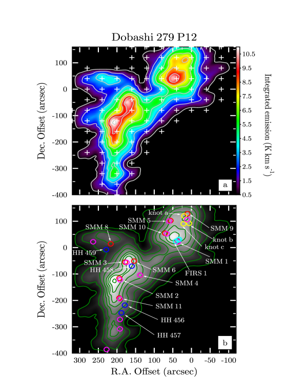
Figure 4: (a): Same as Fig. 1a but for the source Do279P12. The contour levels start at 0.5 K km s^-1 and increments are 1.5 K km s^-1. (b): NH₃(1,1) intensity map as in panel a and positions of IR sources. Open circles mark the Herbig-Haro objects (blue), far-infrared continuum sources (red and yellow) (Davis et al. 1999), submm-continuum sources (magenta) detected by SCUBA (Di Francesco et al. 2008), and the triple radio source FIRS 1 (cyan) (Snell & Bally 1986).

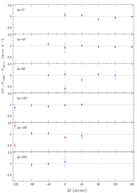
Figure 6: Dots with $3\sigma$ error bars mark the differences between the radial velocities measured with the Effelsberg 100-m telescope in 1977-1981 (Ungerechts & Güsten 1984) and in the present dataset toward the same positions in Do279P12. The red points indicate deviations from zero which are larger than $3\sigma$. At two offsets, $(\Delta\alpha,\Delta\delta)=(80^{\prime\prime},0^{\prime\prime})$ and $(160^{\prime\prime},-120^{\prime\prime})$, we detected double NH₃ profiles (see Fig. 14).

The results of our Effelsberg observations are shown in Figs. 4-6. The NH₃(1,1) map (Fig. 4) exhibits a complex structure with three bright peaks, $T_{\scriptscriptstyle\rm MB}\sim 3$ K, located NW–SE at the offsets $\alpha=(160^{\prime\prime},-40^{\prime\prime})$, $\beta=(200^{\prime\prime},-120^{\prime\prime})$, and $\gamma=(40^{\prime\prime},40^{\prime\prime})$ (see Table 1 and Fig. 5, panel B). The $\alpha$ peak lies very close to the maximum of the NH₃ emission detected by Little et al. (1980), whereas the $\beta$ and $\gamma$ peaks are spatially coincident with positions of the two peaks localized by Ho & Barrett (1980). The measured NH₃ profiles show in this case a double structure in both the (1,1) and (2,2) transitions at four positions (Fig. 14, Table 5) and a split (1,1) line at another three positions where the (2,2) line was not detected. This multicomponent structure has not been resolved previously in the ammonia observations cited above. Since the splitting is also seen in the optically thin ammonia lines, the observed asymmetry of the NH₃ profiles has clearly a kinematic origin.

We used a two-component model, Eq. (13), to fit the data. The result is illustrated in Fig. 14 by the red lines, the detected velocity subcomponents are labeled by letters $A$ and $B$. The seven offsets with the split NH₃ lines are marked by white crosses on the velocity maps shown in Fig. 5. The cluster of the white crosses at the SE part of Do279P12 outlines a small area of the bipolar outflow with an angular extent of $\sim 40^{\prime\prime}\times 80^{\prime\prime}$. Table 5 displays the physical parameters estimated at different offsets. The mean radial velocities of the components A and B averaged over the seven offsets are $\langle V_{\rm A}\rangle=7.27\pm 0.11$ km s^-1 and $\langle V_{\rm B}\rangle=8.54\pm 0.08$ km s^-1, and the velocity difference is $\Delta V_{\scriptscriptstyle\rm B-A}=1.3\pm 0.1$ km s^-1. Panel $A$ in Fig. 5 shows that the gas surrounding the SE double component region has predominantly a negative radial velocity with respect to $\langle V_{\scriptscriptstyle\rm LSR}\rangle$, whereas the gas shown in panel $B$ has a positive $V_{\scriptscriptstyle\rm LSR}$. The observed velocities converge to the mean $\langle V_{\scriptscriptstyle\rm LSR}\rangle$ at the cloud’s outskirts.

Figure 5 shows also a velocity gradient along the E–W direction around the isolated double component region at $(80^{\prime\prime},0^{\prime\prime})$ with $V_{\rm A}=7.89$ km s^-1 and $V_{\rm B}=8.92$ km s^-1. The adjoint regions at $(120^{\prime\prime},0^{\prime\prime})$ and $(40^{\prime\prime},0^{\prime\prime})$ have intermediate velocities of $V_{\scriptscriptstyle\rm LSR}=8.14$ and 8.42 km s^-1, respectively, which become closer to the mean radial velocity of the cloud $\langle V_{\scriptscriptstyle\rm LSR}\rangle=8.099$ km s^-1 at larger offsets: $V_{\scriptscriptstyle\rm LSR}=7.90$ and 8.04 km s^-1 at $(280^{\prime\prime},0^{\prime\prime})$ and $(-40^{\prime\prime},0^{\prime\prime})$, respectively.

The measurement of the excitation temperatures reveals $T_{\rm ex}$ essentially lower than $T_{\rm rot}$ at all 23 offsets listed in Table 5. As discussed above, this may indicate clumpiness of the ammonia distribution and $\eta<1$. In Fig. 4b, we also show the Herbig-Haro (HH) objects and far-infrared continuum sources taken from Davis et al. (1999), the submm-continuum sources detected by SCUBA (Di Francesco et al. 2008), and the position of the triple radio source FIRS 1 (Snell & Bally 1986) which coincides with the brightest infrared object SMM1. The closest position of the split NH₃ lines to the bipolar outflow in FIRS 1 is $(80^{\prime\prime},0^{\prime\prime})$ which corresponds to a projected angular distance of $\theta=45^{\prime\prime}$ from the SE knot of the radio source FIRS 1 (see also Fig. 13 in Snell & Bally 1986). All other splittings are located in the vicinity of the $\beta$ peak, around the SMM2 and SMM11 sources.

The observed linewidths $\Delta v$ of the split NH₃ components are in the range between 0.62 km s^-1 and 0.90 km s^-1. However, larger linewidths ($\Delta v\;\raise 1.29167pt\hbox{$>$\kern-7.5pt\raise-4.73611pt\hbox{$\sim$}}\;1.0$ km s^-1) measured at different offsets (Table 5) may imply unresolved subcomponents of the ammonia lines due to the moderate spectral resolution of our database. Gas flows and jets usually accompany the mass accretion processes in YSOs and protostars. From this point of view the split and/or widened line profiles of NH₃, — a tracer of the dense cores, — may indicate the first stages of the accretion processes in protostars, where jets of HH objects have not yet been formed.

It may be illustrative to compare our $V_{\scriptscriptstyle\rm LSR}$ values with those measured with the same telescope and beam size in 1977-1981 (Ungerechts & Güsten 1984). In total, we have 29 overlapping positions shown in Fig. 6. The calculated differences $\Delta V=V_{1981}-V_{2011}$ are marked by dots with $3\sigma$ error bars. The red points indicate deviations from zero which are larger than $3\sigma$. At two positions, $(\Delta\alpha,\Delta\delta)=(80^{\prime\prime},0^{\prime\prime})$ and $(160^{\prime\prime},-120^{\prime\prime})$, we detected double NH₃ profiles. Among these 29 positions, significant deviations from zero are revealed at 6 offsets, but other points show no variations over this time scale. The ammonia line splitting was not seen at $(80^{\prime\prime},0^{\prime\prime})$ in 1981, although the linewidth was $\Delta v_{1981}=0.85\pm 0.20$ km s^-1, which is comparable to that given in Table 5. However, at $(160^{\prime\prime},-120^{\prime\prime})$ the linewidth was $\Delta v_{1981}=1.68\pm 0.17$ km s^-1, i.e., two times larger than the value from Table 5. We note that the weighted mean of the linewidth at the overlapping positions is $\langle\Delta v\rangle_{1981}=0.93$ km s^-1, and the dispersion of the sample is $\sigma_{\Delta v}=0.18$ km s^-1. The enhanced $\Delta v$(NH₃) at $(160^{\prime\prime},-120^{\prime\prime})$ observed 30 years ago was probably caused by the unresolved structure of the ammonia lines. The maximum deviation $\Delta V_{\scriptscriptstyle\rm LSR}\sim 1$ km s^-1 (Fig. 6) constrains the gas acceleration in an outflow at the level of $\dot{V}\;\raise 1.29167pt\hbox{$<$\kern-7.5pt\raise-4.73611pt\hbox{$\sim$}}\;0.03$ km s^-1 yr^-1. This means that the high-velocity ammonia emission up to $\sim 30-40$ km s^-1 from the line center, observed, for example, in FIRS 1 (Curiel et al. 1996), could be reached in a period of $\sim 1000$ yr. This is comparable to the typical time scale of $10^{3}$ yr — a scale for the episodic ejection of material from protostars (e.g., Ioannidis & Froebrich 2012). The mass of the protostar should be $\;\raise 1.29167pt\hbox{$<$\kern-7.5pt\raise-4.73611pt\hbox{$\sim$}}\;0.3M_{\odot}$ in order to eject the gas clump at the 40 AU radius with the acceleration $\dot{V}\sim 0.03$ km s^-1 yr^-1.

3.5 Dobashi~321~P2 (Do321~P2)

The source Dobashi~321~P2 (Do321P2, herein) is a filamentary dark cloud with the opacity class 6 in accord with Lynds (1962). The cloud is known under the names L673 (Lynds 1962), BDN~46.22-1.34 (Bernes 1977), or P77 (Parker 1988). Do321P2 was observed in ammonia lines by Anglada et al. (1997) and Tobin et al. (2011).

Our NH₃ observations are shown in Fig. 7. The ammonia structure consists of five main subcondensations. Their reference positions are listed in Table 1. The brightest $\alpha$ and $\beta$ peaks with $T_{\scriptscriptstyle\rm MB}\sim 3$ K are located near the sources IRAS 19180+1114 (SMM2) and IRAS 19180+1116 (SMM1), respectively. The ammonia peak detected by Anglada et al. has an offset $(-123^{\prime\prime},83^{\prime\prime})$ and is resolved into two clumps $\alpha$ and $\beta$ in our observations (see Fig. 7). We also detected three weaker ammonia clumps $\gamma$, $\delta$, and $\varepsilon$ with $T_{\scriptscriptstyle\rm MB}\sim 1.7,1.6$, and 1.3 K, respectively. The $\gamma$ and $\varepsilon$ condensations, localized within the confines of the older map of Anglada et al. (1997), peak near the source IRAS 19181+1112, whereas the $\delta$ clump was not resolved by Anglada et al. (1977) because of a too coarse angular resolution.

Interferometric observations of a small region around SMM2 ($\sim 100^{\prime\prime}\times 100^{\prime\prime}$) in lines of N₂H⁺ and NH₃ (Tobin et al. 2011; see Fig. 14) show a substantial amount of extended ammonia emission which closely traces the spacial distribution of N₂H⁺. The measured NH₃ radial velocity $V_{\scriptscriptstyle\rm LSR}$ = 6.93 km s^-1, the linewidth $\Delta v=0.50$ km s^-1, and the column density $N$(NH₃) = $7.2\times 10^{14}$ cm^-2 (Table 8 in Tobin et al.) are in a good agreement with our values for the $\alpha$ peak (Table 1): $V_{\scriptscriptstyle\rm LSR}$ = 6.88 km s^-1, $\Delta v=0.49$ km s^-1, and $N$(NH₃) = $6\times 10^{14}$ cm^-2. However, the estimates of the excitation temperature at this position contradict sharply: $T_{\rm ex}$ = 33.3 K (Tobin et al.) and 6.8 K (our value from Table 3). We detected NH₃(1,1) and (2,2) at the $\alpha$ and $\beta$ peaks (Fig. 15). Their profiles are well described by a single-component model (red lines in Fig. 15, model parameters are given in Table 3). Both spectra show the same $T_{\rm ex}$, which is also consistent with the values measured in other dense molecular cores (see Tables 4-6).

The NH₃ velocity map (Fig. 7b) shows irregular structure with distinct pockets of redshifted and blueshifted ammonia emission around the clusters of YSOs at the positions of SMM1 and SMM2 (Fig. 7c). The observed kinematics are caused by large-scale motions in this star-forming region which cannot be interpreted unambiguously.

The apparent diameters (beam deconvolved) of the two NH₃ condensations $d_{\alpha}=60^{\prime\prime}$ and $d_{\beta}=40^{\prime\prime}$ and the gas densities listed in Table 3 allow us to estimate masses of these clumps assuming spherical geometry: $M_{\alpha}\sim 0.3M_{\odot}$, and $M_{\beta}\sim 0.1M_{\odot}$. The relative ammonia abundance in both clumps is [NH₃]/[H₂] $\sim 2\times 10^{-7}$. We note that the corresponding virial masses of these clumps are considerably larger ($M^{\alpha}_{\rm vir}\sim 2M_{\odot}$, and $M^{\beta}_{\rm vir}\sim 1M_{\odot}$) and probably affected by the masses of YSOs embedded in the cloud.

3.6 Kawamura~05 (Ka05)

The source Kawamura~05 (Ka05, herein) is a Bok globule of the opacity class 6 (Lynds 1962). The cloud is known under the names B335 (Barnard 1927), L663 (Lynds 1962), or CB199 (Clemens & Barvainis 1988). Being the prototype of an isolated, star-forming dark cloud, B335 has been studied at many wavelengths.

Single-pointing ammonia observations towards B335 were carried out by Ho et al. (1977, 1978), Myers & Benson (1983), Benson & Myers (1989), and Levshakov et al. (2010). The first mapping of this core in the NH₃(1,1) and (2,2) lines with the Effelsberg telescope revealed an elongated N-S structure (Menten et al. 1984, M84 herein). The kinetic temperature measured at four positions, where the NH₃(2,2) line was observed, is uniformly distributed over the core region, $T_{\rm kin}$ = 10-12 K.

We mapped the core Ka05 at nine offsets around the reference point $\alpha$(J2000) = 19:37:01.3, $\delta$(J2000) = +07:34:29.6 which is shifted off the center position in M84 at $(\Delta\alpha,\Delta\delta)=(-24.0^{\prime\prime},-42.8^{\prime\prime})$. The results of our observations are shown in Fig. 8. Two positions $(0^{\prime\prime},0^{\prime\prime})$ and $(0^{\prime\prime},-40^{\prime\prime})$ with $T_{\scriptscriptstyle\rm MB}$ = 2.5 K and 2.1 K (Table 1) coincide, respectively, with the offsets $(20^{\prime\prime},40^{\prime\prime})$ with $T_{\scriptscriptstyle\rm MB}$ = 3.4 K and $(20^{\prime\prime},0^{\prime\prime})$ with $T_{\scriptscriptstyle\rm MB}$ = 2.8 K in M84. In between these positions, at $(20^{\prime\prime},20^{\prime\prime})$, the brightness temperature was even higher, $T_{\scriptscriptstyle\rm MB}$ = 4.1 K (M84), but we did not observe this point with our larger step size of $40^{\prime\prime}$, as well as the point $(20^{\prime\prime},60^{\prime\prime})$ where $T_{\scriptscriptstyle\rm MB}$ = 3.1 K. However, we measured NH₃(1,1) at $(0^{\prime\prime},40^{\prime\prime})$ with $T_{\scriptscriptstyle\rm MB}$ = 0.6 K which corresponds to the point $(20^{\prime\prime},80^{\prime\prime})$ not listed in Table 1 in M84. The opposite marginal point $(20^{\prime\prime},-20^{\prime\prime})$ along the cut $\Delta\alpha=20^{\prime\prime}$ in M84 has $T_{\scriptscriptstyle\rm MB}$ = 0.8 K. This indicates sharp drops of the brightness temperature at the edges of the disk-like envelope surrounding the protostar.

The spectra with the measured (1,1) and (2,2) lines are shown in Fig. 16. The radial velocities at two offsets $(0^{\prime\prime},0^{\prime\prime})$ and $(0^{\prime\prime},-40^{\prime\prime})$ are the same as they were in 1982/83 (cf. Fig. 6, Sect. 3.4, where velocity shifts at some positions in the map of Do279P12 were detected for the same three decades). The linewidths (Table 3) are also consistent with M84. At these offsets, the measured kinetic temperatures, excitation temperatures, total optical depths, and column densities are in line with M84.

The NH₃(1,1) velocity map is shown in Fig. 8b. The velocity distribution resembles a rigid body rotation with the tangential velocity increasing from $\approx-0.040$ km s^-1 (NE) to $\approx+0.040$ km s^-1 (SW) at cloud flanks. The radius of the NH₃ disk-like envelope is about $40^{\prime\prime}$ in accord with our and the M84 maps. The distance to B335 was recently redetermined to be only $D=90-120$ pc (Olofsson & Olofsson 2009). This gives us a radius $r\sim 0.02$ pc, and an angular velocity $\dot{\phi}\sim(6-8)\times 10^{-15}$ s^-1 ($\beta\;\raise 1.29167pt\hbox{$<$\kern-7.5pt\raise-4.73611pt\hbox{$\sim$}}\;0.001$), which is close to the value of M84, $\dot{\phi}\sim 1.5\times 10^{-14}$ s^-1. The corresponding stability parameter $\beta^{\prime}\approx 2\times 10^{-4}$. With the apparent diameter $d\sim 0.04$ pc, the relative abundance ratio is [NH₃]/[H₂] $\sim 4\times 10^{-7}$.

To compare with previous estimates of the mass of the gas giving rise to ammonia emission, we assume spherical geometry and for the gas density $n_{{\rm H}_{2}}\sim 2\times 10^{4}$ cm^-3 (Table 3) to obtain $M\sim 0.05M_{\odot}$ — 40 times lower than the value reported by Benson & Myers (1989) who used a core radius $R=0.11$ pc ($D=250$ pc) and a gas density $n_{{\rm H}_{2}}\sim 6\times 10^{3}$ cm^-3.

If the centrifugal forces prevent the disk-like structure from collapse, then the mass of the center source is given, within a factor of 2, by (e.g., Frerking & Langer 1982):

$$M_{c}=V^{2}_{t}R/G,$$ (6)

where $R$ is the distance of the material from the source and $G$ is the gravitational constant. For $V_{t}=0.040$ km s^-1, it gives $M_{c}\sim 0.03M_{\odot}$. This estimate indicates that Ka05 is a low-mass protostellar source which agrees with the measurement of the central source mass $M_{c}\sim 0.04M_{\odot}$ from SMA observations of the C¹⁸O(2-1) emission (Yen et al. 2010).

3.7 Dobashi~279~P7 (Do279~P7)

The dense molecular cloud Dobashi~279~P7 (Do279P7, herein) is the next example of a starless core from our list. This is a newly discovered dense clump which is so far poorly studied. No embedded IRAS sources or pre-main-sequence stars are known within $80^{\prime\prime}$ off the core center. The NH₃(1,1) intensity distribution shown in Fig. 9 has approximately circular symmetry. The half-power dimension of the core is $80^{\prime\prime}\times 80^{\prime\prime}$, or, correcting for our beam, $70^{\prime\prime}\times 70^{\prime\prime}$, i.e., the source is resolved in both right ascension and declination. Assuming a distance to the source of $D\approx 203$ pc (see Sect. 1), its radius is about 0.03 pc. The parameters for the density peak at $(-80^{\prime\prime},40^{\prime\prime})$ are given in Table 1. The NH₃ spectra are shown in Fig. 17. We detected the (2,2) transition at four positions which allow us to estimate $T_{\rm rot}$ $=11.5-13.5$ K and $T_{\rm kin}$ = $12.4-14.9$ (Table 3). These values exceed slightly the temperatures measured in the starless core Ka01, but the linewidths in Do279P7, are significantly larger than the linewidths in Ka01 and Do279P8 – another starless core but without detected (2,2) transition (see Table 3). The wider lines in Do279P7 indicate a higher level of turbulence in this core with the ratio of turbulent to thermal velocity dispersion of $\Delta v_{\rm turb}/\Delta v_{\rm th}\approx 5$. The profiles of the NH₃(1,1) hfs components do not show any blueward or redward asymmetry indicating contracting or expanding motions. However, the NH₃ intensity map shows a filament-like structure in the S-E direction (P.A. $\approx 135^{\circ}$) with $V_{\scriptscriptstyle\rm LSR}$ $\sim 0.8$ km s^-1 (Fig. 9).

The core exhibits a linear velocity gradient from the southern ($V_{\scriptscriptstyle\rm LSR}$ $\sim 0.0$ km s^-1) to the northern edge ($V_{\scriptscriptstyle\rm LSR}$ $\sim-0.8$ km s^-1) that can be interpreted as rigid body rotation around the axis $\Delta\delta\approx 20^{\prime\prime}$, P.A. $\approx 90^{\circ}$ (Fig. 9b). The measured tangential velocity of $\pm 0.4$ km s^-1 at $r\approx 0.03$ pc leads to an angular velocity of $\dot{\phi}\approx 5\times 10^{-13}$ s^-1. With $n_{{\rm H}_{2}}\sim 1\times 10^{4}$ cm^-3 (Table 3) and assuming spherical geometry, one obtains a core mass of $M\sim 0.2M_{\odot}$. The estimates of the angular velocity and the gas density give $\beta\sim 6$ which shows that the rotation energy is larger or comparable to the gravitational energy of this starless core. The parameter $\beta^{\prime}\approx 0.3$ is also rather high as compared with other isolated cores Ka01, Do279P8, and Ka05 where $\beta^{\prime}\ll 1$. The measured column density $N\sim 6\times 10^{14}$ cm^-2 and the linear size $d\sim 0.06$ pc indicate a relative ammonia abundance of [NH₃]/[H₂] $\sim 3\times 10^{-7}$.

3.8 Serpens South 3 (SS3)

The source Serpens South 3 (SS3, herein) is a dense core located in an active star-forming region discovered by Gutermuth et al. (2008) in Spitzer IRAC mid-infrared imaging of the Serpens-Aquila rift. The central part of this region, near $\alpha$ = 18^h 30^m 03^s, $\delta$ = $-02^{\circ}$ 01^′ 58.2^′′ (J2000), which is called Serpens South, is composed of 37 Class I and 11 Class II sources at high mean surface density ($>430$ pc^-2) and short median nearest neighbor spacing (0.02 pc). The overall structure of the star-forming region exhibits a typical filamentary dense gas distribution elongated for about $14^{\prime}$ in the NW-SE direction.

For the first time, we mapped the core SS3 in the NH₃(1,1) and (2,2) lines around the reference point $\alpha$ = 18^h 29^m 57.1^s, $\delta$ = $-02^{\circ}$ 00^′ 10.0^′′ (J2000) in the area $\Delta\alpha\times\Delta\delta=160^{\prime\prime}\times 360^{\prime\prime}$ (Fig. 10). The nominal center of the NH₃ map is shifted by $2^{\prime}29^{\prime\prime}$ (P.A. $\approx-40^{\circ}$) with respect to the center of Box 1 in the CO map of Nakamura et al. (2011, herein N11) and coincides with the intensity peak of the CO outflow lobe marked by ${\it R2}$ in N11. The angular size of the CO lobe within the 15 K km s^-1 contour is about $70^{\prime\prime}\times 60^{\prime\prime}$ (Figs. 9 and 15 in N11), and the whole region lies in the lowest NH₃ intensity ‘valley’ running in E-W direction along the cut $\Delta\delta=0^{\prime\prime}$ in Fig. 10. To the south of this valley, at $\Delta\delta\approx-140^{\prime\prime}$, an intensity peak of NH₃ ($\alpha$ peak in Table 1 and Fig. 10b) occurs at the northern part of another CO outflow lobe marked ${\it R3}$ in N11. These two redshifted lobes ${\it R2}$ and ${\it R3}$ appear to have the blueshifted counterparts ${\it B1}$ and ${\it B4}$ originating from a compact 3 mm source — a deeply embedded, extremely young Class 0 protostar (N11). It is interesting to note that the configuration of the NH₃ valley just follows the lowest dust emission distribution on the 1.1 mm continuum image of this area shown in Fig. 15(b) in N11. To the north and to the south of the valley there are regions of relatively strong 1.1 mm emission which are correlated with strong NH₃ emission. The three NH₃ peaks $\alpha,\beta$, and $\gamma$ listed in Table 1 and labeled in Fig. 10b have very high brightness temperatures $T_{\scriptscriptstyle\rm MB}$ = 5.0, 3.1, and 3.0 K.

Examples of the observed NH₃(1,1) and (2,2) spectra are shown in Fig. 18. Here again, as was the case of the core Do279P12, we find split NH₃ profiles. The apparent asymmetry of the ammonia lines is observed in optically thin hf components and, thus, cannot be due to radiative transfer effects (self-absorption). The components $A$ and $B$, detected at two offsets (see Table 6), have the radial velocities $\langle V_{\rm A}\rangle=7.865\pm 0.005$ km s^-1 and $\langle V_{\rm B}\rangle=6.856\pm 0.010$ km s^-1. The map of the velocity field is shown in Fig. 10b where the positions of the split NH₃ profiles are labeled by the white crosses. The closest Class 0 protostar to these positions is the MAMBO mm source MM10 (Maury et al. 2011) marked by the yellow circle in Fig. 10c at the offset $(38^{\prime\prime},-53^{\prime\prime})$. However, since the whole region is very complex, it is not clear which source drives this presumably bipolar molecular outflow causing the observed splitting of the NH₃ profiles.

The measured linewidths listed in Table 6 show that the values $\Delta v\;\raise 1.29167pt\hbox{$>$\kern-7.5pt\raise-4.73611pt\hbox{$\sim$}}\;0.8$ km s^-1 are symmetrically distributed around the positions of the split NH₃ profiles in the E-W strip of about $120^{\prime\prime}$ width, cut by the vertical edges of our map. The strip of enhanced linewidths (see Fig. 22) may be associated with the E-W bipolar outflow, thus giving rise to the local redshifted and blueshifted patches of the velocity map shown in Fig. 10b.

It is seen from Table 6 that the values of the measured parameters fluctuate considerably from one position to another. Namely, the excitation temperature ranges from 3.3 K to 8.4 K, $T_{\rm rot}$ — from 8.6 K to 14.8 K, $T_{\rm kin}$ — from 8.9 K to 16.8 K, the gas density $n_{{\rm H}_{2}}$ — from $0.3\times 10^{4}$ cm^-3 to $4.2\times 10^{4}$ cm^-3, the total optical depth $\tau_{11}$ — from 1.5 to 20.0, and the column density $N$(NH₃) — from $0.2\times 10^{15}$ cm^-2 to $2.8\times 10^{15}$ cm^-2. We note that the highest gas density of $n_{{\rm H}_{2}}\sim 4.2\times 10^{4}$ cm^-3 was measured at two positions where we observed the split NH₃ lines profiles. The largest optical depths with $13.2\;\raise 1.29167pt\hbox{$<$\kern-7.5pt\raise-4.73611pt\hbox{$\sim$}}\;\tau_{11}\;\raise 1.29167pt\hbox{$<$\kern-7.5pt\raise-4.73611pt\hbox{$\sim$}}\;20.0$ are localized along the N–S cut $\Delta\alpha=0^{\prime\prime}$ between $\Delta\delta=80^{\prime\prime}$ and $200^{\prime\prime}$ which passes through the $\gamma$ and $\beta$ peaks in the region where three starless core candidates (red circles in Fig. 10c) were detected by Maury et al. (2011). The maximum (16.6 K and 16.8 K) and minimum (8.9 K) kinetic temperatures are observed along the N–S cut at $\Delta\alpha=80^{\prime\prime}$. The minimum of the kinetic temperature correlates with the minimum of the brightness temperature, $T_{\scriptscriptstyle\rm MB}$= 0.5 K, whereas $T_{\scriptscriptstyle\rm MB}$= 1.2 K at $T_{\rm kin}$= 16.8 K (the foot of the $\alpha$ peak) and $T_{\scriptscriptstyle\rm MB}$= 5.0 K at $T_{\rm kin}$= 16.6 K (the top of the $\alpha$ peak). This gradient of $T_{\rm kin}$ ($8.9-16.8$ K) is probably due to the presence of two YSOs localized at the top and foot of the $\alpha$ peak shown in Fig. 10b.

3.9 Dobashi 243 P2, 279 P18, 279 P13, and 321 P1

The sources Do243P2, Do279P18, Do243P13, and Do321P1 (Table 1) were observed at their central positions and at $40^{\prime\prime}$ offsets toward the four cardinal directions. Only a weak NH₃(1,1) emission ($T_{\scriptscriptstyle\rm MB}$ $\;\raise 1.29167pt\hbox{$<$\kern-7.5pt\raise-4.73611pt\hbox{$\sim$}}\;1$ K) is seen toward each of them. The corresponding spectra are depicted in Fig. 19. For Do321P1, two possible detections of the ammonia emission are shown at the bottom panels, but the noise is high and the identification of the NH₃(1,1) line is not certain. The measured radial velocity of $V_{\scriptscriptstyle\rm LSR}$ = 13.5 km s^-1 for Do321P1 is somewhat larger than that measured for the other sources from Table 1 for which $V_{\scriptscriptstyle\rm LSR}$ ranges between 6.0 km s^-1 and 9.6 km s^-1, however, the ¹²CO(1-0) 115.3 GHz, ¹³CO(1-0) 110.2 GHz, and C¹⁸O(1-0) 109.8 GHz emission lines were also detected at $V_{\scriptscriptstyle\rm LSR}$ $\sim 13$ km s^-1 with the Delingha 14-m telescope (Wang 2012).

No submillimeter-continuum sources have been found within $2^{\prime}$ off the core centers of Do279P18, Do243P13, and Do321P1, but a SCUBA point-like source J180447.8-043208 (Di Francesco et al. 2008) lies in the field of Do243P2 at the angular distance $\theta=41^{\prime\prime}$, P.A. = $-30^{\circ}$ from the nominal center $(0^{\prime\prime},0^{\prime\prime})$.

3.10 Sources without detected NH₃ emission

A list of 37 targets from our dataset with undetected NH₃ emission is presented in Table 2. Columns 3 and 7 give the noise level per channel width of 0.077 km s^-1 on a $T_{\scriptscriptstyle\rm MB}$ scale and the mapped area, respectively. In the fields of some targets there were found the following objects.

Do279P21: a point-like infrared source IRAS 18191-0310 (Cutri et al. 2003) at $\theta=80^{\prime\prime}$, P.A. = $-174^{\circ}$.

Do279P17: a point-like infrared source IRAS 18351+0010 (Cutri et al. 2003) at $\theta=17^{\prime\prime}$, P.A. = $74^{\circ}$.

Do296P3: a point-like submillimeter-continuum source J185121.1-041714 (Di Francesco et al. 2008) at $\theta=29^{\prime\prime}$, P.A. = $-173^{\circ}$.

Ka15: a galaxy gJ194852.5-103056 (Skrutskie et al. 2006) at $\theta=64^{\prime\prime}$, P.A. = $99^{\circ}$.

Ka17: a point-like infrared IRAS 19470-0630 (Porras et al. 2003) at $\theta=57^{\prime\prime}$, P.A. = $162^{\circ}$.

4 Summary

We have used the Effelsberg 100-m telescope to observe the NH₃(1,1) and (2,2) spectral lines in high density molecular cores. The targets were preliminarily selected from the CO and ¹³CO survey of the Aquila rift cloud complex carried out with the Delingha 14-m telescope. We measured a minimum grid of 5 positions with $40^{\prime\prime}$ spacing centered upon the $(0^{\prime\prime},0^{\prime\prime})$ position determined from the maximum intensity of the CO maps. We mapped a larger area for sources where ammonia emission was detected to delineate the spatial distribution of NH₃.

In total, we have mapped the first 49 CO sources (from $\sim 150$ targets) and detected 12 NH₃ emitters what gives an overall detection rate of $\sim 24$ per cent which is 3 times lower as compared to the Pipe Nebula which was observed with the GBT 100-m telescope (Rathborne et al. 2008) and which is not too far from the clouds studied here (see Sect. 1). The NH₃ sources in our sample represent diverse populations of molecular clouds from isolated and homogeneous starless cores with suppressed turbulence to star formation regions with complex intrinsic motion and gas density fluctuations.

The starless cores Ka01, Do279P8, Do279P7, Do279P18, Do243P13, and a candidate — the clump $\varepsilon$ Do279P6 — have radial velocities $V_{\scriptscriptstyle\rm LSR}$ ranging from 6.0 km s^-1 to 9.6 km s^-1 with the mean $\langle$$V_{\scriptscriptstyle\rm LSR}$$\rangle$ = 8.1 km s^-1, and dispersion $\sigma=1.2$ km s^-1. The only starless core with $V_{\scriptscriptstyle\rm LSR}$ beyond the $3\sigma$ interval around the mean is Do321P1 for which $V_{\scriptscriptstyle\rm LSR}$ = 13.5 km s^-1. Three cores — Ka01, Do279P8, and the clump $\varepsilon$ Do279P6 — demonstrate rather narrow linewidths, $\Delta v\;\raise 1.29167pt\hbox{$<$\kern-7.5pt\raise-4.73611pt\hbox{$\sim$}}\;0.4$ km s^-1, whereas the others have $\Delta v\sim 0.5-1$ km s^-1. The masses of the starless cores do not exceed a solar mass and are typically $(0.1-0.5)M_{\odot}$, except for the cores $\varepsilon$ Do279P6, Do279P8, and Ka05 for which $M<0.1M_{\odot}$. The measured ammonia abundance, $X=$ [NH₃]/[H₂], ranges between $1\times 10^{-7}$ and $5\times 10^{-7}$ with the mean $\langle X\rangle=(2.7\pm 0.6)\times 10^{-7}$.

For three cores — Ka01, Do279P8, and Ka05 — we measured low angular velocities (parameters $\beta$ and $\beta^{\prime}\ll 1$) and their rotation energies are less than the gravitational energy, but Do279P7 — a fast rotator — yields a rotational energy comparable to the gravitational energy ($\beta\approx 6$ and $\beta^{\prime}\approx 0.3$). It also has a high ratio of the turbulent to thermal velocity.

Two isolated star-forming cores, Ka05 and Do243P2, were observed. The cores’ radial velocities are $V_{\scriptscriptstyle\rm LSR}$ = 8.4 km s^-1 and 7.0 km s^-1, respectively, and, thus, both of them belong to the same group of cores with $V_{\scriptscriptstyle\rm LSR}$ $\sim 8$ km s^-1. For the former core, we estimate a sub-solar mass and thus confirm that Ka05 is a low-mass protostellar source. Both cores exhibit narrow linewidths, $\Delta v\sim 0.3$ km s^-1.

Most intense ammonia emission was observed towards four clouds with complex gas density and velocity structures which harbor numerous YSOs: Do279P6, Do279P12, Do321P2, and SS3. Each of them consists of a number of clumps with different angular sizes. The $\langle$$V_{\scriptscriptstyle\rm LSR}$$\rangle$ values show that the complex clouds have the same radial velocities as the starless cores and isolated star-forming clouds from our dataset. It is only one cloud —Do279P12 — where the dispersion of bulk motions is comparable to the ammonia linewidths. The internal bulk motions in the other three clouds are less pronounced and show lower dispersions as compared to the NH₃ linewidths.

Kinematically split NH₃ profiles were detected in Do279P12 and SS3. The velocity splitting is $\sim 1$ km s^-1. In the former object, the splitting is most probably caused by bipolar molecular outflows observed in other molecular lines. This object has been observed in ammonia lines with the Effelsberg telescope three decades ago. We compared these observations with the current spectra and found velocity shifts at some positions which correspond to an acceleration of the gas flow of $\dot{V}\;\raise 1.29167pt\hbox{$<$\kern-7.5pt\raise-4.73611pt\hbox{$\sim$}}\;0.03$ km s^-1 yr^-1.

The measured kinetic temperatures lie between 9 K and 12 K for the starless and isolated star-forming sources, except for the fast rotator Do279P7 where $T_{\rm kin}$ ranges between 12 K and 15 K. An increased value of $T_{\rm kin}$ in this case may be due to magnetic energy dissipation since magnetic and nonthermal energy densities may be nearly equal in Do279P7: for $n=1.1\times 10^{4}$ cm^-3, $v=0.4$ km s^-1, and assuming $B\sim 20\leavevmode\nobreak\ \mu$G we obtain $B^{2}/8\pi\approx\rho v^{2}/2\sim 2\times 10^{-11}$ dyn cm^-2. However, to what extent the magnetic energy dissipation contributes to the gas heating requires further investigations.

For the complex filamentary dark clouds, $T_{\rm kin}$ varies between 9 K and 18 K and strongly fluctuates from point to point. We found no simple relationship between gas density and kinetic temperature. High density condensations in the filamentary dark clouds have a large range of temperatures, most probably determined by radiation from embedded stars and dust.

For the beam filling factor $\eta=1$, we estimated the excitation temperature of an inversion doublet, the ammonia column densities, and H₂ densities for those clouds where both the (1,1) and (2,2) transitions were detected. The typical values of $T_{\rm ex}$ lie between 3 K and 8 K, the total NH₃ column densities between $0.3\times 10^{15}$ cm^-2 and $3\times 10^{15}$ cm^-2, and H₂ volume densities between $0.3\times 10^{4}$ cm^-3 and $4.2\times 10^{4}$ cm^-3.

The study of Aquila dense cores will be continued, with the remaining $\sim 100$ targets scheduled for observations at the Effelsberg 100-m telescope in 2013.

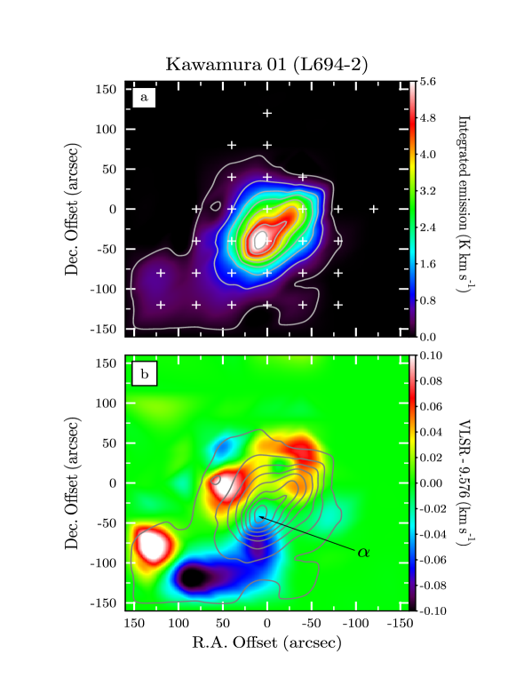
Figure 1: (a): NH₃(1,1) intensity map ($\int$$T_{\scriptscriptstyle\rm MB}$$dv$) of Ka01. The starting point for the contour levels is 0.1 K km s^-1, the increment is 0.7 K km s^-1 between the first two and 0.8 K km s^-1 between the other contour levels. The crosses mark measured positions. (b): NH₃(1,1) radial velocity (color map) structure. The velocity field is shown after subtraction of the mean radial velocity $\langle V_{\scriptscriptstyle\rm LSR}\rangle=9.576$ km s^-1. The intensity peak is labeled in accord with Table 1. The Effelsberg beam size (HPBW) at 23.7 GHz is $40^{\prime\prime}$.

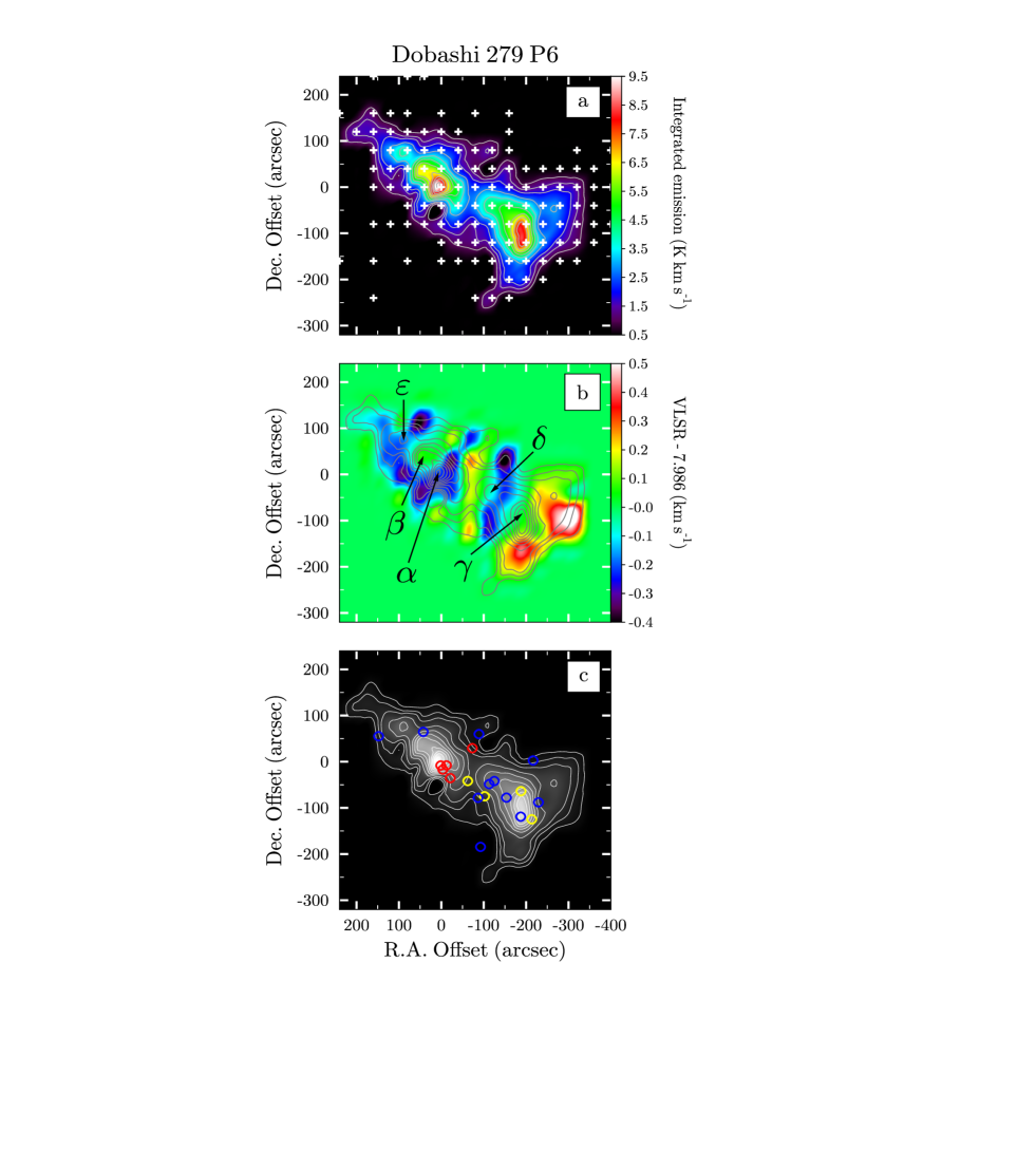
Figure 2: (a): Same as Fig. 1a but for the source Do279P6. The starting point for the contour levels is 0.5 K km s^-1, the increment is 0.5 K km s^-1 between the first two and 1.0 K km s^-1 between the other contour levels. (b): NH₃(1,1) radial velocity (color map) structure. The velocity field is shown after subtraction of the mean radial velocity $\langle V_{\scriptscriptstyle\rm LSR}\rangle=7.986$ km s^-1. The intensity peaks are labeled in accord with Table 1. (c): NH₃(1,1) intensity map as in panel a and positions of YSO candidates observed with the Spitzer/IRAC in a star formation region Serpens cluster B (Harvey et al. 2006). Open circles of different colors mark Class I (red), intermediate type (yellow), and Class II (blue) YSOs.

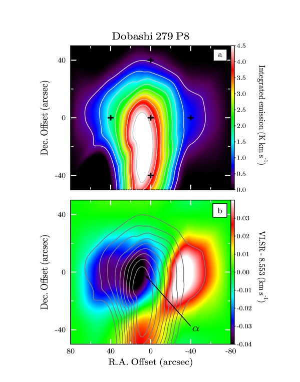
Figure 3: (a): Same as Fig. 1a but for the source Do279P8. The contour levels start at 0.5 K km s^-1 and increments are 0.5 K km s^-1. (b): NH₃(1,1) radial velocity (color map) structure. The velocity field is shown after subtraction of the mean radial velocity $\langle V_{\scriptscriptstyle\rm LSR}\rangle=8.553$ km s^-1. The intensity peak is labeled in accord with Table 1.

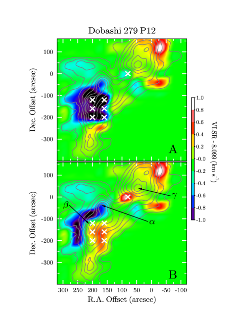
Figure 5: NH₃(1,1) intensity (grey contours) and radial velocity (color map) structure in the source Do279P12. The velocity field is shown after subtraction of the mean radial velocity $\langle V_{\scriptscriptstyle\rm LSR}\rangle=8.099$ km s^-1. The contour levels are the same as in Fig. 4a. Panels A and B represent the velocity maps for the components A and B in the NH₃ profile, respectively (see Fig. 14). The white crosses mark offsets where the splitting of the NH₃ profiles is detected. The mean radial velocities of the components A and B are $\langle V_{\rm A}\rangle=7.27\pm 0.11$ km s^-1 and $\langle V_{\rm B}\rangle=8.54\pm 0.08$ km s^-1. In panel B, the intensity peaks are labeled in accord with Table 1.

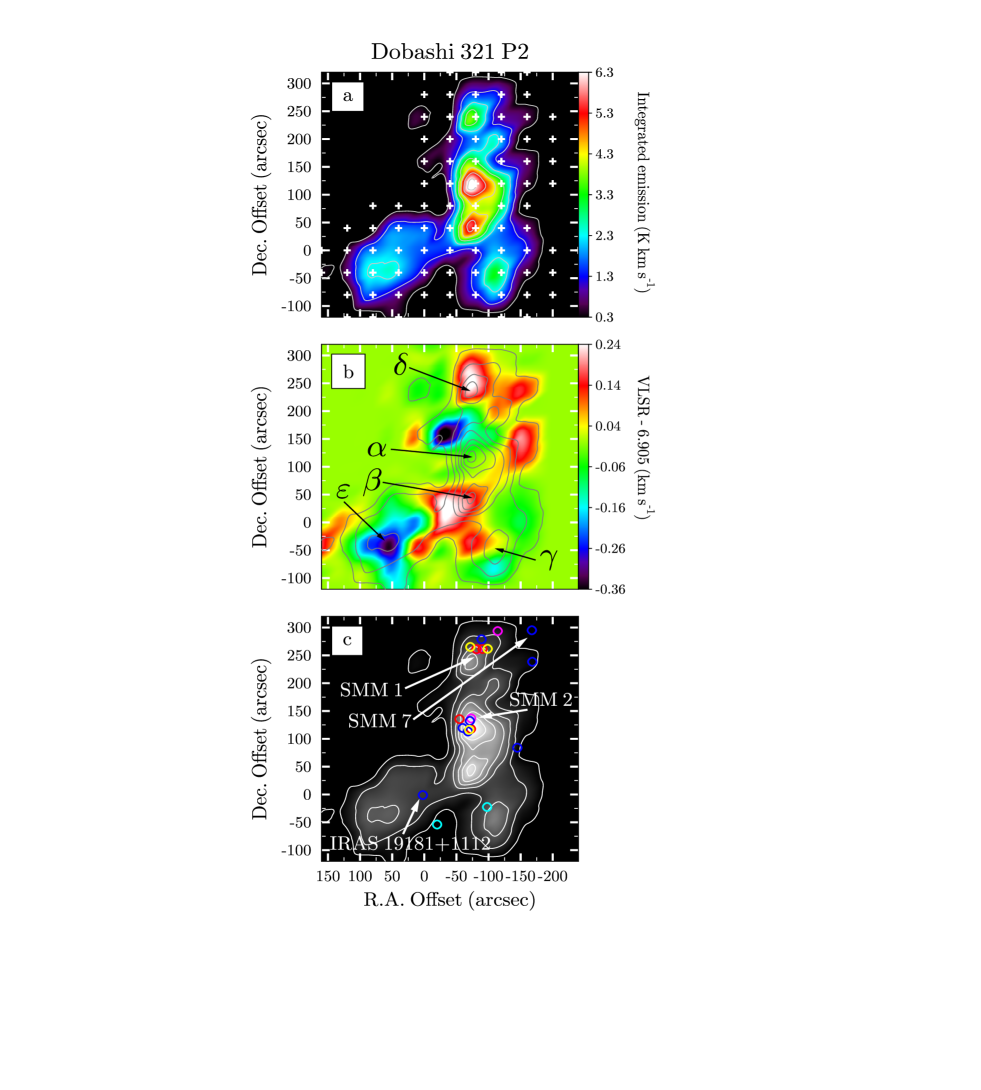
Figure 7: (a): Same as Fig. 1a but for the source Do321P2. The contour levels start at 0.3 K km s^-1 and increments are 1.0 K km s^-1. (b): NH₃(1,1) radial velocity (color map) structure. The velocity field is shown after subtraction of the mean radial velocity $\langle V_{\scriptscriptstyle\rm LSR}\rangle=6.905$ km s^-1. The intensity peaks are labeled in accord with Table 1. (c): NH₃(1,1) intensity map as in panel a. Open circles of different colors mark Class I (red), intermediate type (yellow), Class II (blue), and Class III (cyan) YSOs taken from Tsitali et al. (2010). The SCUBA sources from Visser et al. (2002) are marked by magenta: SMM7 is a starless core, whereas SMM1 and SMM2 are protostars which coincide with IRAS 19180+1116 and IRAS 19180+1114, respectively.

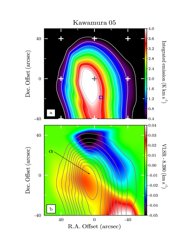
Figure 8: (a): Same as Fig. 1a but for the source Ka05. The contour levels start at 0.4 K km s^-1 and increments are 1.0 K km s^-1. The square indicates the position of the far-infrared source IRAS 19345+0727 coinciding with the 3.6 cm continuum source (Anglada et al. 1992). (b): NH₃(1,1) radial velocity (color map) structure. The velocity field is shown after subtraction of the mean radial velocity $\langle V_{\scriptscriptstyle\rm LSR}\rangle=8.390$ km s^-1. The intensity peak is labeled in accord with Table 1.

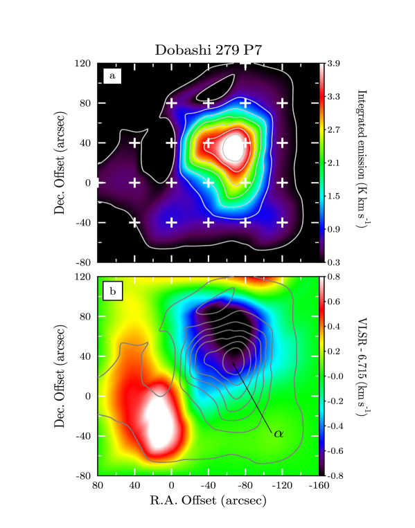
Figure 9: (a): Same as Fig. 1a but for the source Do279P7. The contour levels start at 0.3 K km s^-1 and increments are 0.6 K km s^-1. (b): NH₃(1,1) radial velocity (color map) structure. The velocity field is shown after subtraction of the mean radial velocity $\langle V_{\scriptscriptstyle\rm LSR}\rangle=6.715$ km s^-1. The intensity peak is labeled in accord with Table 1.

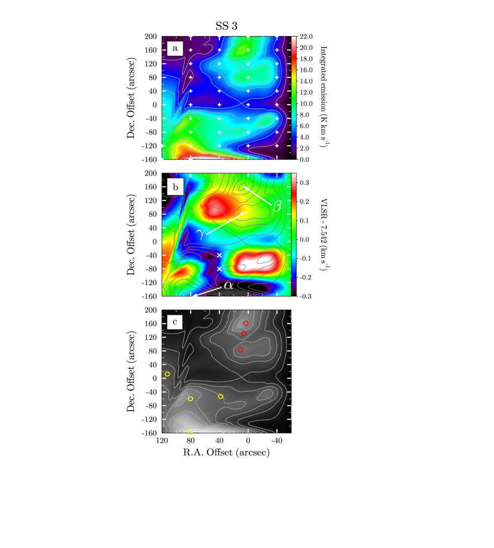
Figure 10: (a): Same as Fig. 1a but for the source SS3. The contour levels start at 0.0 K km s^-1 and increments are 2.0 K km s^-1. (b): NH₃(1,1) radial velocity (color map) structure. The velocity field is shown after subtraction of the mean radial velocity $\langle V_{\scriptscriptstyle\rm LSR}\rangle=7.542$ km s^-1. The white crosses mark offsets where the splitting of the NH₃ profiles is detected (see Fig. 18). The mean radial velocities of the components A and B are $\langle V_{\rm A}\rangle=7.865\pm 0.005$ km s^-1 and $\langle V_{\rm B}\rangle=6.856\pm 0.010$ km s^-1. The intensity peaks are labeled in accord with Table 1. (c): NH₃ intensity map as in panel a and positions of the MAMBO millimeter sources taken from Table 1 in Maury et al. (2011). Red and yellow open circles mark starless and YSO candidates, respectively.

Table 1: Peak intensities of NH₃(1,1) line emission toward Aquila targets

Source	Peak	Position		Offset		$T_{\scriptscriptstyle\rm MB}$b	$V_{\scriptscriptstyle\rm LSR}$	$\Delta v^{c}$		Date	Other name
	Id.a	$\alpha_{2000}$	$\delta_{2000}$	$\Delta\alpha$,	$\Delta\delta$	(K)	(km s-1)	(km s-1)		(d-m-y)
		(h: m: s)	(°: ′: ″)	(″),	(″)
Do243~P2	$\alpha$	18:04:49	$-$04:32:38	$40$,	$0$	0.30(6)	6.97(1)	0.	39(6)	30-03-11	J180447.8-0432081
Do279~P6	$\alpha$	18:29:07	+00:30:51	$0$,	$0$	2.9(6)	7.75(1)	0.	753(7)	26,29-03-11	Ser G3-G62
	$\beta$			$40$,	$40$	2.1(4)	8.04(1)	0.	63(1)	26,29-03-11
	$\gamma$			$-160$,	$-80$	1.8(4)	7.69(1)	0.	96(3)	26,29-03-11
	$\delta$			$-120$,	$-40$	1.7(3)	7.91(1)	0.	7(1)	26,29-03-11
	$\varepsilon$			$80$,	$80$	1.3(2)	7.81(1)	0.	4(1)	26,29-03-11
Do279~P12	$\alpha$	18:29:47	+01:14:53	$160$,	$-40$	3.2(6)	7.59(1)	0.	90(3)	28-03-11	BDN~31.57+5.373
	$\beta$			$200$,	$-120$	2.8(6)	7.09(1)	0.	84(3)	28-03-11
	$\gamma$			$40$,	$40$	2.9(6)	8.29(1)	0.	91(2)	28-03-11
SS3	$\alpha$	18:29:57	$-$02:00:10	$80$,	$-160$	5(1)	7.39(1)	1.	140(9)	13-01-12
	$\beta$			$0$,	$160$	3.1(6)	7.62(1)	0.	396(4)	13-01-12
	$\gamma$			$0$,	$80$	3.0(6)	7.67(1)	0.	488(6)	12-01-12
Do279~P8	$\alpha$	18:30:04	$-$02:48:14	$0$,	$0$	2.5(5)	8.52(1)	0.	26(2)	30-03-11
Do279~P7	$\alpha$	18:31:08	$-$02:10:22	$-80$,	$40$	1.5(3)	6.04(1)	0.	74(2)	12-01-12	BDN~28.65+3.663
Do279~P18	$\alpha$	18:36:48	$-$01:13:27	$0$,	$0$	0.20(4)	8.53(1)	1.	1(1)	28-03-11
Do279~P13	$\alpha$	18:39:15	+00:28:50	$-40$,	$0$	1.0(2)	8.26(1)	0.	51(3)	28-03-11
Do321~P1	$\alpha$	18:57:10	+00:52:58	$-40$,	$0$	0.15(3)	13.6(1)	0.	30(3)	29-03-11
	$\beta$			$0$,	$40$	0.10(2)	13.5(1)	1.	0(2)	29-03-11
Do321~P2	$\alpha$	19:20:31	+11:17:56	$-80$,	$120$	3.0(6)	6.88(1)	0.	49(1)	29-03-11	BDN~46.22–1.34,
	$\beta$			$-80$,	$40$	2.7(6)	7.06(1)	0.	43(1)	29-03-11	L673, P773
	$\gamma$			$-120$,	$-40$	1.7(3)	6.93(1)	0.	38(2)	29-03-11
	$\delta$			$-80$,	$240$	1.6(3)	7.12(1)	0.	47(2)	29-03-11
	$\varepsilon$			$80$,	$-40$	1.3(3)	6.66(1)	0.	73(5)	29-03-11
Ka05	$\alpha$	19:37:01	+07:34:30	$0$,	$0$	2.5(5)	8.40(1)	0.	365(8)	12-01-12	B3354, CB1995
Ka01	$\alpha$	19:41:04	+10:57:17	$0$,	$-40$	2.5(5)	9.55(1)	0.	311(8)	28-03-11	B1434, L694–26
Notes. aGreek letters mark peaks of ammonia emission indicated in Figs. 1-3, 5, 7-10.
bThe number in parentheses correspond to a $1\sigma$ statistical error at the last digital position. cLinewidth (FWHM).
References. (1) Di Francesco et al. 2008; (2) Cohen & Kuhi 1979; (3) Dobashi et al. 2005; (4) Barnard 1927;
(5) Clemens and Barvainis 1988; (6) Lee and Myers 1999.

Table 2: Molecular cores toward Aquila targets without detected NH₃ emission in the (1,1) and (2,2) inversion transitions

No.	Source	rmsa	Position		Date	Mapped area	Other name
		(K)	$\alpha_{2000}$	$\delta_{2000}$	(d-m-y)	$\Delta\alpha\times\Delta\delta$
			(h: m: s)	(°: ′: ″)		(″) (″)
1	Do243 P3	0.24	18:03:07	$-$04:52:30	30-03-11	$80\times 80$
2	Do243 P1	0.23	18:03:51	$-$04:29:33	29,30-03-11	$80\times 80$
3	Do243 P6	0.22	18:08:43	$-$03:25:03	30-03-11	$80\times 80$
4	Do243 P8	0.24	18:13:48	$-$03:15:20	30-03-11	$80\times 80$
5	Do243 P7	0.24	18:16:21	$-$03:24:49	30-03-11	$80\times 80$
6	Do279 P19	0.24	18:21:00	$-$03:01:10	30-03-11	$40\times 80$
7	Do279 P21	0.24	18:21:45	$-$03:07:36	30-03-11	$80\times 80$
8	Do279 P27	0.22	18:23:43	$-$03:14:34	28-03-11	$80\times 80$
9	Do279 P25	0.26	18:25:34	$-$02:54:04	30-03-11	$80\times 80$
10	Do279 P2	0.19	18:26:59	$-$03:43:44	28-03-11	$80\times 80$
11	Do279 P3	0.23	18:28:21	$-$03:29:20	30-03-11	$80\times 80$
12	Do279 P5	0.24	18:28:42	$-$03:44:58	30-03-11	$80\times 80$
13	Do279 P14	0.26	18:29:15	$-$03:19:38	30-03-11	$80\times 80$
14	Do279 P22	0.24	18:29:18	$-$01:25:33	30-03-11	$80\times 80$
15	Do279 P4	0.24	18:30:09	$-$03:42:28	30-03-11	$80\times 80$
16	Do279 P1	0.24	18:31:31	$-$02:30:29	30-03-11	$80\times 80$
17	Do279 P24	0.22	18:33:20	+00:42:42	30-03-11	$80\times 80$	LND5831
18	Do279 P17	0.24	18:37:41	+00:13:06	28-03-11	$80\times 80$
19	Do279 P20	0.24	18:38:29	$-$00:02:30	30-03-11	$80\times 80$
20	Do296 P3	0.18	18:51:21	$-$04:16:45	28-03-11	$80\times 80$
21	Do321 P8	0.22	18:55:36	+02:12:00	28-03-11	$80\times 80$
22	Do321 P5	0.22	19:01:38	+04:05:11	30-03-11	$80\times 80$
23	Do299 P1	0.19	19:07:31	$-$03:55:48	29-03-11	$80\times 80$	B1352
24	Do321 P7	0.23	19:10:48	+07:26:14	30-03-11	$80\times 80$
25	Ka09	0.20	19:35:11	+12:25:40	30-03-11	$80\times 80$
26	Ka03	0.21	19:40:36	+10:20:14	30-03-11	$80\times 80$	LDN6901
27	Ka16	0.15	19:43:08	$-$05:42:04	28,30-03-11	$320\times 320$
28	Ka19	0.26	19:43:15	$-$07:13:44	30-03-11	$80\times 80$
29	Ka02	0.23	19:44:10	+10:28:28	30-03-11	$80\times 80$
30	Ka21	0.19	19:45:11	$-$07:07:41	28-03-11	$80\times 80$
31	Ka06	0.17	19:47:50	+10:50:16	28-03-11	$80\times 80$
32	Ka07	0.15	19:48:48	+11:23:07	28-03-11	$80\times 80$	B3402
33	Ka15	0.27	19:48:48	$-$10:30:46	30-03-11	$80\times 80$
34	Ka17	0.23	19:49:44	$-$06:21:44	30-03-11	$80\times 80$
35	Ka14-15-A	0.30	19:51:49	$-$10:34:32	30-03-11	$120\times 80$
36	Ka14	0.32	19:51:58	$-$10:32:12	29,30-03-11	$80\times 80$
37	Ka23	0.27	19:58:36	$-$14:06:00	30-03-11	$80\times 80$	MBM1593
Notes. aMean noise level per channel width of 0.077 km s-1 on a $T_{\scriptscriptstyle\rm MB}$ scale.
References. (1) Lynds 1962; (2) Barnard 1927; (3) Magnani et al. 1985.

Appendix A The analysis of NH₃(1,1) and (2,2) spectra

In this Appendix we discuss the methods used for calculating physical parameters from observations of the ammonia NH₃ $(J,K)=(1,1)$ and (2,2) transitions. We give a consistent summary of the basic formulae relevant to the study of cold molecular cores.

The recorded NH₃ spectra were first converted into the $T_{\scriptscriptstyle\rm MB}$ scale and a baseline was removed from each of them. The baseline was typically linear in the range covered by the ammonia hyperfine (hf) structure lines but occasionally quadratic. After that the spectra of the same offset were co-added with weights inversely proportional to the mean variance of the noise per channel, rms^-2, estimated from the channels with no emission.

The NH₃ spectra were fitted to determine the total optical depth $\tau_{\rm tot}$ in the respective inversion transition, the LSR velocity of the line $V_{\scriptscriptstyle\rm LSR}$, the intrinsic full width to half power linewidth $\Delta v$ for an individual hf component, and the amplitude, $\cal{A}$ (e.g., Ungerechts et al. 1980):

$$T(v)={\cal A}\left[1-{\rm e}^{-\tau(v)}\right]\,.$$ (7)

The optical depth $\tau(v)$ at a given radial velocity $v$ is defined by

$$\tau(v)=\tau_{\rm tot}\sum^{n}_{i=1}r_{i}\exp\{-2.77[(v-V_{\scriptscriptstyle\rm LSR})+v_{i}]^{2}/(\Delta v)^{2}\}.$$ (8)

In this equation, the sum runs over the $n$ hf components of the inversion transition ($n=18$ and 21 for the NH₃(1,1) and (2,2) inversion transitions, respectively), $r_{i}$ is the theoretical relative intensity of the $i$th hf line and $v_{i}$ is its velocity separation from the fiducial frequency. The values of these parameters are given in, e.g., Kukolich (1967) and Rydbeck et al. (1977).

In Eq.(8), the total optical depth, $\tau_{\rm tot}$, is the maximum optical depth which an unsplit (1,1) or (2,2) line would have at the central frequency if the hf levels were populated at the same excitation temperature for both lines (1,1) and (2,2). Assuming that the line profile function has a Gaussian shape with the width $\Delta v$ (FWHM) and taking into account that the statistical weights of the upper and lower levels of an inversion transitions are equal, one obtains

$$\tau_{\rm tot}(J,K) = \frac{16\pi^{3}\mu^{2}}{3h\Delta v}\left(\frac{\ln 2}{\pi}\right)^{1/2}\frac{K^{2}}{J(J+1)}N(J,K)\cdot$$ (9)

$$\cdot\frac{1-\exp(-h\nu/k_{\scriptscriptstyle\rm B}T_{\rm ex})}{1+\exp(-h\nu/k_{\scriptscriptstyle\rm B}T_{\rm ex})}\,,$$

where $h$ and $k_{\scriptscriptstyle\rm B}$ are Planck’s and Boltzmann’s constants, respectively, $\mu$ is the dipole moment, $|\mu|=1.4719$ Debye (JPL catalog), $N(J,K)$ is the inversion state column density — the sum of the column densities of the upper and lower levels of an inversion doublet, $\nu$ is the rest frequency of the inversion transition, and $T_{\rm ex}$ is the excitation temperature which characterizes the NH₃ population across the $(J,K)$ inversion doublet.

In Eq.(7), the amplitude ${\cal A}$ can be expressed in terms of the beam filling factor, $\eta=\Omega_{\rm cloud}/\Omega_{\rm beam}$ (solid angle $\Omega=\pi\theta^{2}/(4\ln 2)$, where $\theta$ is the angular diameter at FWHP), and the excitation temperature, $T_{\rm ex}$, as

$${\cal A}=\eta\left[J_{\nu}(T_{\rm ex})-J_{\nu}(T_{\rm bg})\right]\,,$$ (10)

where $T_{\rm bg}=2.7$ K is the black body background radiation temperature, and $J_{\nu}(T)$ is defined by

$$J_{\nu}(T)=\frac{h\nu}{k_{\scriptscriptstyle\rm B}}\left({\rm e}^{h\nu/k_{\scriptscriptstyle\rm B}T}-1\right)^{-1}.$$ (11)

For optically thin lines (e.g., $\tau_{11}\ll 1$), Eq.(7) degenerates into

$$T(v) = {\cal A}\cdot\tau(v)$$ (12)

$$= ({\cal A}\tau_{11})\cdot\sum^{n}_{i=1}r_{i}\exp[-2.77(\Delta V_{i}/\Delta v)^{2}]\,,$$

and it is not possible to determine ${\cal A}$ and $\tau_{11}$ separately. Here $\Delta V_{i}=v-V_{\scriptscriptstyle\rm LSR}+v_{i}$.

For some molecular cores we observe two-component NH₃ profiles. The line parameters $\{{\cal A}_{j},\tau^{(j)}_{\rm 11},\tau^{(j)}_{\rm 22},V^{(j)}_{\scriptscriptstyle\rm LSR},\Delta v_{j}\}$ for both $j=1$ and $j=2$ components were determined in this case by fitting the function

$$T(v)=T_{1}(v)+T_{2}(v)\,.$$ (13)

This linear form assumes that two clouds in the beam have the same filling factor $\eta$ and the same $T_{\rm ex}$ for both lines (1,1) and (2,2).

At low spectral resolutions, when the channel spacing, $\Delta_{\rm ch}$, is comparable to the linewidth $\Delta v$, the derived line parameters are affected by the channel profile $\phi(v)$. In this case, the recorded spectrum, $T^{\prime}(v)$, was considered as a convolution of the true spectrum $T(v)$ and $\phi(v)$

$$T^{\prime}(v)=\int T(v)\cdot\phi(v-v^{\prime})\,dv^{\prime}\,.$$ (14)

We approximate $\phi(v)$ by a Gaussian function with the width FWHM defined by a particular backend setting.

The calculated synthetic spectrum which is defined as $T_{\rm syn}(v)\equiv T(v)$ if $\Delta_{\rm ch}\ll\Delta v$, or $T_{\rm syn}(v)\equiv T^{\prime}(v)$ if $\Delta_{\rm ch}\sim\Delta v$, was fitted to the observed spectrum $T_{\rm obs}(v)$ through minimization of the $\chi^{2}$ function

$$\chi^{2}=\sum\,\left[T_{\rm syn}(v)-T_{\rm obs}(v)\right]^{2}/{\rm rms}^{2}$$ (15)

in the 5-dimensional space of the following model parameters: ${\cal A},\tau_{\rm 11},\tau_{\rm 22},V_{\scriptscriptstyle\rm LSR},$ and $\Delta v$. Attempting to exclude at the $3\sigma$ level all noise-only channels in between the hf lines, the sum runs over the channels with observed NH₃ emission from all hf components. The minimum of $\chi^{2}$ was computed using the simplex method (e.g., Press et al. 1992).

Equation (15) was also used to estimate the formal errors of the model parameters through calculation of the covariance matrix at the minimum of $\chi^{2}$. Since the uncertainty in the amplitude scale calibration was $\sim$15-20% (Sect. 2), and there were no noticeable correlations between the sequential channels in our datasets, we did not correct the calculated errors by an additional factor as described, e.g., in Rosolowsky et al. (2008).

Given the estimate of the amplitude ${\cal A}$, the excitation temperature $T_{\rm ex}$ can be calculated from Eq.(10):

$$T_{\rm ex}=\frac{T_{0}}{\ln\left[1+T_{0}\eta/({\cal A}+\eta J_{\rm bg})\right]}\,,$$ (16)

where $T_{0}=h\nu/k{\scriptscriptstyle\rm B}$, and $J_{\rm bg}=J_{\nu}(T_{\rm bg})$. At $T_{\rm bg}=2.725$ K and NH₃-inversion frequencies, we have $J_{\rm bg}=2.20$ K and $T_{0}=1.14$ K.

In this equation the only unknown parameter is the filling factor, $\eta$. If the source is completely resolved, then $\eta=1$. Otherwise, Eq. (16) gives a lower bound on $T_{\rm ex}$ corresponding to $\eta=1$, whereas decreasing $\eta$ drives $T_{\rm ex}$ towards its upper bound at $T_{\rm ex}$ = $T_{\rm kin}$, which holds for LTE. In case of emission, the radiation temperature within the line is larger than the 2.7 K background and the excitation may be either radiative or collisional. At gas densities larger than the critical density and for optically thin lines the local density of line photons is negligible as compared to the background radiation field, and the lower metastable states in NH₃ are mainly populated via collisions with molecular hydrogen, i.e., the stimulated emission can be neglected. For low collisional excitation, $n_{\rm gas}<n_{\rm cr}$, the line radiation controls $T_{\rm ex}$ for both optically thin and thick regimes (Kegel 1976). NH₃(1,1) emission usually arises from regions with $n_{\rm gas}\;\raise 1.29167pt\hbox{$>$\kern-7.5pt\raise-4.73611pt\hbox{$\sim$}}\;10^{4}$ cm^-3 (e.g., Ho & Townes 1983). It means that the regime of low collisional excitation does not dominate. We also do not consider anomalous excitation (maser emission), leading to $T_{\rm ex}$ $\gg T_{\rm bg}$, since masing is not observed in our data sample. Thus, the use of $T_{\rm ex}$ = $T_{\rm kin}$ as a formal upper limit for the excitation temperature is legitimate. By this we can restrict the unknown filling factor for an unresolved source in the interval

$$\eta_{\rm min}\leq\eta\leq\eta_{\rm max}\ ,$$ (17)

and $T_{\rm ex}$ within the boundaries

$$\left.T^{\rm min}_{\rm ex}\right|_{\eta=1}\leq T_{\rm ex}\leq\left.T^{\rm max}_{\rm ex}\right|_{\eta=\eta_{\rm min}}\ .$$ (18)

From a separate analysis of the (1,1) and (2,2) lines with low noise level, we found that both amplitudes ${\cal A}_{11}$ and ${\cal A}_{22}$ are equal within the observational errors, which implies that $T_{\rm ex}(1,1)\approx T_{\rm ex}(2,2)$. Albeit radiative transfer calculations show that the excitation temperatures $T_{\rm ex}(1,1)$ and $T_{\rm ex}(2,2)$ may differ by about 20% (Stutzki & Winnewisser 1985), the assumption of their equivalence seems to be sufficiently good in our case.

The second temperature which describes the NH₃ population is the rotational temperature, $T_{\rm rot}$, characterizing the population of energy levels with different $(J,K)$. As mentioned above, the population of the lower metastable inversion doublets is determined by collisions with H₂ and, thus, is regulated by the kinetic temperature, $T_{\rm kin}$. The population ratio between the (1,1) and (2,2) states is defined as

$$\frac{N_{22}}{N_{11}}=\frac{g_{22}}{g_{11}}\cdot\exp\left(-\frac{\Delta E_{12}}{k_{\scriptscriptstyle\rm B}T_{\rm rot}}\right)=\frac{5}{3}\cdot\exp\left(-\frac{41.5{\rm K}}{T_{\rm rot}}\right).$$ (19)

Assuming that both transitions trace the same volume of gas and their linewidths $\Delta v$ are equal, one finds from Eqs.(9) and (19) that

$$T_{\rm rot}=-41.5/\ln\left(\frac{9}{20}\cdot\frac{\tau_{22}}{\tau_{11}}\right)\,.$$ (20)

We note that since radiative transitions between the different $K$-ladders of the $(J,K)$ levels are forbidden and that the unknown filling factor $\eta$ is canceled in the line intensity ratio of the NH₃ (1,1) and (2,2) transitions, the estimate of the rotational temperature is more reliable than the excitation temperature.

For a two-level system with the kinetic temperature less than the energy gap between the (1,1) and (2,2) states ($\Delta E_{12}=41.5$ K), the rotational temperature can be related to the kinetic temperature through detailed balance arguments (e.g., Ragan et al. 2011):

$$T_{\rm kin}=T_{\rm rot}/[1-\frac{T_{\rm rot}}{\Delta E_{12}}\cdot\ln(1+1.1\ {\rm e}^{-15.7/T_{\rm rot}})]\ .$$ (21)

The beam-averaged column density $N_{\scriptscriptstyle JK}$ (in cm^-2) can be calculated from Eqs.(9) and (10) using the estimated values of the amplitude ${\cal A}$, the total optical depth $\tau_{\scriptscriptstyle JK}$, and the linewidth $\Delta v$:

$$N_{\scriptscriptstyle JK}=\zeta_{\scriptscriptstyle JK}\cdot\Delta v\cdot\tau_{\scriptscriptstyle JK}\cdot\frac{{\cal A}+\eta(J_{\rm bg}+0.5T_{0})}{\eta}\ ,$$ (22)

where $\zeta_{\scriptscriptstyle 11}=1.3850\times 10^{13}$, $\zeta_{\scriptscriptstyle 22}=1.0375\times 10^{13}$, and $\Delta v$ is in km s^-1 (for detail, see Ungerechts et al. 1980). As mentioned above, ${\cal A}_{11}\approx{\cal A}_{22}$, and for both transitions $T_{0}=1.14$ K, and $J_{\rm bg}=2.20$ K. Substituting these numerical values in Eq.(22), one obtains

$$N_{11}=3.84\times 10^{13}\cdot\Delta v\cdot\tau_{\scriptscriptstyle 11}\cdot(1+{\cal A}/2.77\eta)\ .$$ (23)

This gives us lower and upper boundaries of $N_{11}$ if $\eta\in[\eta_{\rm min},1]$ :

$$\left.N^{\rm min}_{11}\right|_{\eta=1}\leq N_{11}\leq\left.N^{\rm max}_{11}\right|_{\eta=\eta_{\rm min}}.$$ (24)

The uncertainty interval $\Delta N_{11}=N^{\rm max}_{11}-N^{\rm min}_{11}$ transforms directly into the estimate of the total NH₃ column density:

$$N({\rm NH}_{3}) = N_{11}\cdot[(1/3)\exp(23.2/T_{\rm rot})+1+$$ (25)

$$+(5/3)\exp(-41.5/T_{\rm rot})+$$

$$+(14/3)\exp(-105.2/T_{\rm rot})+\ldots]\ ,$$

which assumes that the relative population of all metastable levels of both ortho-NH₃ ($K=3$), which is not observable, and para-NH₃  ($K=1,2$) is governed by the rotational temperature of the system at thermal equilibrium (Winnewisser et al. 1979). Substituting $N^{\rm min}_{11}$ and $N^{\rm max}_{11}$ from (24) into (25), one finds:

$$\left.N({\rm NH}_{3})_{\rm min}\right|_{\eta=1}\leq N({\rm NH}_{3})\leq\left.N({\rm NH}_{3})_{\rm max}\right|_{\eta=\eta_{\rm min}}.$$ (26)

The detailed balance calculations also provide a relation between the gas density, gas kinetic temperature, and the excitation temperature (e.g., Ho & Townes 1983):

$$n({\rm H}_{2})=\frac{A}{C}\left[\frac{J_{\nu}(T_{\rm ex})-J_{\nu}(T_{\rm bg})}{J_{\nu}(T_{\rm kin})-J_{\nu}(T_{\rm ex})}\right]\left[1+\frac{J_{\nu}(T_{\rm kin})}{h\nu/k_{\scriptscriptstyle\rm B}}\right],$$ (27)

where $A$ is the Einstein A-coefficient, and $C$ is the rate coefficient for collisional de-excitation. For a typical kinetic temperature in the dense molecular cores of $\sim 10-20$ K, the collision coefficient is $\sim 4\times 10^{-7}{\rm s}^{-1}\ [n({\rm H}_{2})/10^{4}{\rm cm}^{-3}]$. The value of $A$ for the inversion transition (1,1) is $1.67\times 10^{-7}$ s^-1. However, the gas density calculated using Eq.(27) may be significantly underestimated if the beam is not filled uniformly. Moreover, in case of $T_{\rm ex}$ = $T_{\rm kin}$, Eq.(27) is invalid and, hence, $n({\rm H}_{2})$ is to be calculated by different methods (see, e.g., Hildebrand 1983; Pandian et al. 2012). We use (27) just to set a lower bound on the gas density, $n({\rm H}_{2})_{\rm min}$, at $\eta=1$.

Given a fractional NH₃ abundance, an upper bound on the gas density may be estimated from the deduced $N$(NH${}_{3})_{\rm max}$ assuming that the ammonia emission traces the real distribution of the gas density. If the source is unresolved, its diameter, $d$, and the beam filling factor are related as

$$d=\theta_{\rm m}D\sqrt{\eta}\ ,$$ (28)

where $\theta_{\rm m}$ is the beam angular diameters (FWHP), and $D$ the distance of the source. The highest gas density is obtained at the smallest diameter, $d_{\rm min}=\theta_{\rm m}D\sqrt{\eta_{\rm min}}$ :

$$n({\rm H}_{2})_{\rm max}=\left.\frac{N({\rm NH}_{3})_{\rm max}}{X\cdot d_{\rm min}}\right|_{\eta=\eta_{\rm min}},$$ (29)

where $X=[{\rm NH}_{3}]/[{\rm H}_{2}]$ is a given abundance ratio. In this equation the unknown distance $D$ can be found from the requirement that both values of the lowest gas densities calculated at $\eta=1$ from Eq.(27) and from $N({\rm NH}_{3})_{\rm min}$ at $d_{\rm max}=\theta_{\rm m}D$ be equal. This gives

$$n({\rm H}_{2})_{\rm max}=\frac{n({\rm H}_{2})}{\sqrt{\eta_{\rm min}}}\frac{N({\rm NH}_{3})_{\rm max}}{N({\rm NH}_{3})_{\rm min}}\ .$$ (30)

For the unresolved source its axis — major, $\theta_{\rm a}$, or minor, $\theta_{\rm b}$ — is less than $\theta_{\rm m}$, $\eta<1$, and only limiting values can be obtained for $T_{\rm ex}$, $N_{JK}$, $N({\rm NH}_{3})$, and $n({\rm H}_{2})$. If the source is resolved, i.e., $\theta_{\rm b}>\theta_{\rm m}$, then $\eta=1$ and these physical parameters are directly defined. In the latter case we calculate the deconvolved values of $\theta_{\rm a}$ and $\theta_{\rm b}$ and their geometrical mean

$$\theta=\sqrt{\theta_{\rm a}\cdot\theta_{\rm b}}\ ,$$ (31)

which is used as a formal estimate of the source angular diameter.

A similar procedure is applied to calculate the virial mass of the ammonia core through the linewidth, $\Delta v$. If the observed value $\Delta v$ is of order of the spectral resolution $\Delta_{\rm sp}$ (FWHM), then only an upper limit on $M_{\rm vir}$ is defined. Otherwise, if $\Delta v$ $>\Delta_{\rm sp}$, then the deconvolved value of the linewidth, $\Delta\tilde{v}$, and the core radius $r$ give the virial mass (e.g., Lemme et al. 1996)

$$M_{\rm vir}=250\cdot\Delta\tilde{v}^{2}\cdot r\ ,$$ (32)

where $\Delta\tilde{v}$ is in km s^-1, $r$ in pc, and $M_{\rm vir}$ in solar masses $M_{\odot}$.

To conclude, we note that in some cases, when $T_{\rm kin}$ varies slowly within an ammonia clump, the NH₃ column density can be deduced from the (1,1) line alone assuming the same average $T_{\rm kin}$ in the core as in the outskirts of a cloud. This allows us to extend the radial gas distribution to zones with unobservable (2,2) emission (Morgan et al. 2013).

Appendix B Ammonia spectra toward the Aquila rift cloud complex and derived physical parameters

The observed spectra of the NH₃(1,1) and (2,2) transitions detected at the peak positions of ammonia emission toward each core are shown in Figs. 11-19. The measured physical parameters are listed in Tables 3-6. The distributions of the physical parameters for three most abundant cores are presented in Figs. 20-22. They demonstrate variations of the kinetic temperature, $T_{\rm kin}$, the excitation temperature, $T_{\rm ex}$, the linewidth, $\Delta v$ (FWHM), the total optical depth, $\tau_{11}$, the gas density, $n_{{\rm H}_{2}}$, and the total ammonia column density, $N$(H₂), across the mapped area of the core.

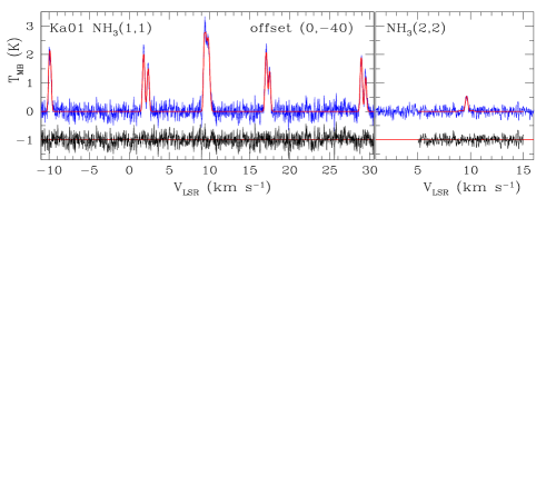
Figure 11: Ammonia (1,1) and (2,2) spectra (blue) toward the source Ka01. The channel spacing is 0.015 km s^-1, the spectral resolution FWHM = 0.024 km s^-1. The red curves show the fit of a single-component Gaussian model to the original data. The residuals between the observed and model spectra are shown by black color.

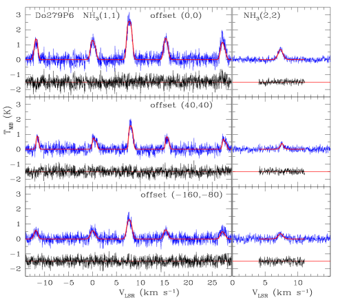
Figure 12: Same as Fig. 11 but for the source Do279P6.

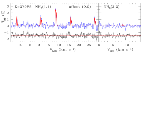
Figure 13: Same as Fig. 11 but for the source Do279P8 and the channel spacing 0.077 km s^-1 (FWHM = 0.123 km s^-1). The red curves show the fit of a single-component Gaussian model to the NH₃(1,1) original data and the upper limit on NH₃(2,2).

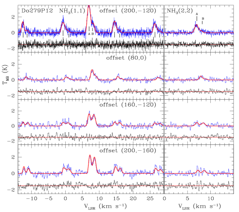
Figure 14: Same as Fig. 11 but for the source Do279P12. The ammonia spectra have double structure. The upper panels show the high-resolution spectra (channel spacing 0.015 km s^-1), and the other panels — low-resolution spectra (channel spacing 0.077 km s^-1). Two NH₃ components are marked by ticks and labeled by letters A and B in the upper panels.

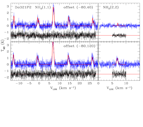
Figure 15: Same as Fig. 11 but for the source Do321P2.

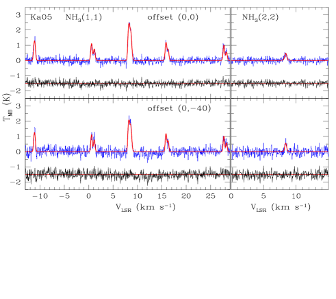
Figure 16: Same as Fig. 11 but for the source Ka05 and the channel spacing 0.038 km s^-1 (FWHM = 0.044 km s^-1).

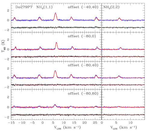
Figure 17: Same as Fig. 16 but for the source Do279P7.

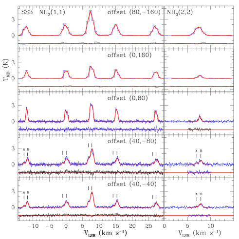
Figure 18: Same as Fig. 11 but for the source SS3. The channel spacing is 0.77 km s^-1 and 0.038 km s^-1 at two upper and three lower panels, respectively. The corresponding spectral resolutions are 0.895 km s^-1 and 0.044 km s^-1 (FWHM). The red curves show the fit of a single-component (two upper panels) and a double-component (three lower panels) Gaussian model to the original NH₃ data. Two components of the NH₃ emission are marked by ticks and labeled by letters A and B.

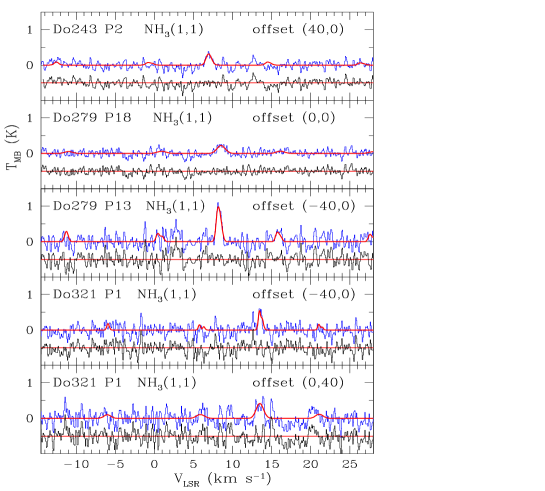
Figure 19: Same as Fig. 13 but for the sources Do243P2, Do279P18, Do279P13, and Do321P1.

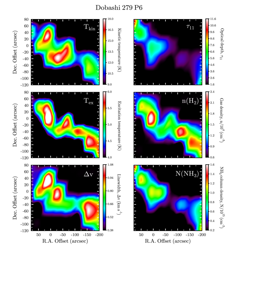
Figure 20: The spatial distributions of the physical parameters measured in Do279P6 from the ammonia inversion lines NH₃(1,1) and (2,2). The corresponding numerical values are listed in Table 4.

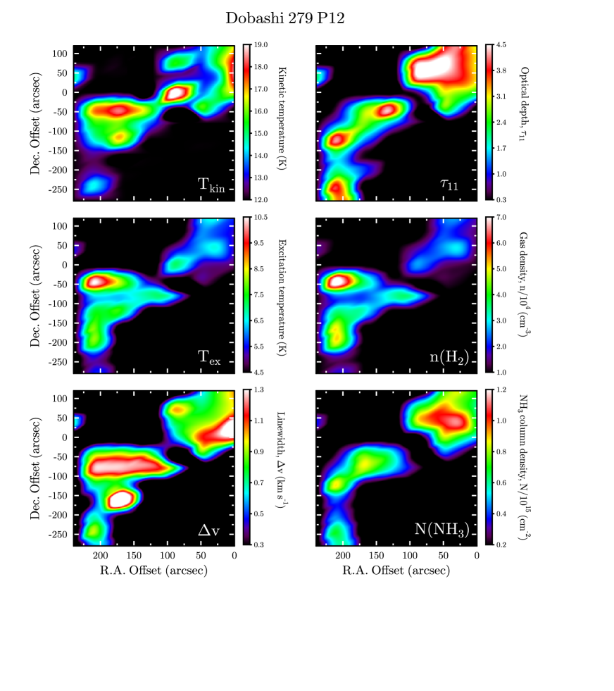
Figure 21: The spatial distributions of the physical parameters measured in Do279P12 from the ammonia inversion lines NH₃(1,1) and (2,2). The corresponding numerical values are listed in Table 5.

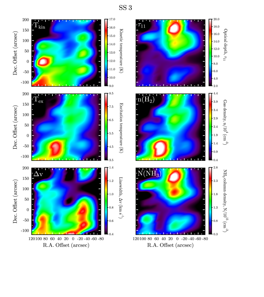
Figure 22: The spatial distributions of the physical parameters measured in SS3 from the ammonia inversion lines NH₃(1,1) and (2,2). The corresponding numerical values are listed in Table 6.

Table 3: Observed parameters of the NH₃(1,1) and (2,2) lines and calculated model parameters for Kawamura~01 and 05, Dobashi 279 P7 and P8, and Dobashi 321 P2

Peak	$\Delta\alpha$	$\Delta\delta$	$V_{\scriptscriptstyle\rm LSR}$	$\Delta v$	$T_{\scriptscriptstyle\rm MB}$	$T_{\rm ex}$	$T_{\rm rot}$	$T_{\rm kin}$	$n_{{\rm H}_{2}}/10^{4}$	$\tau_{11}$	$\tau_{22}$	$N_{\rm tot}/10^{15}$
Id.	$(^{\prime\prime})$	$(^{\prime\prime})$	(km s-1)	(km s-1)	(K)	(K)	(K)	(K)	(cm-3)			(cm-2)
Ka01
	0,	0	9.60	0.32	1.5	4.3	8.7	9.1	1.2	10.9	0.2	1.2
$\alpha$	0,	$-40$	9.55	0.32	2.5	5.5	9.2	9.6	2.5	10.5	0.3	1.3
	+40,	$-40$	9.60	0.30	1.4	4.8	$<8.5$	$\ldots$	$\ldots$	4.1	$<0.1$	$\geq 0.5$
	+40,	$-80$	9.54	0.30	0.8	4.1	$<9.6$	$\ldots$	$\ldots$	3.2	$<0.1$	$\geq 0.3$
	$-40$,	0	9.62	0.23	1.7	4.7	$<8.9$	$\ldots$	$\ldots$	8.2	$<0.2$	$\geq 1.0$
	$-40$,	$-40$	9.60	0.27	1.3	4.3	$<9.7$	$\ldots$	$\ldots$	6.6	$<0.2$	$\geq 0.5$
Ka05
$\alpha$	$0$,	$0$	8.40	0.37	2.5	5.6	10.2	10.7	2.3	5.6	0.3	0.8
	$0$,	$-40$	8.40	0.33	2.1	5.1	10.8	11.5	1.6	8.0	0.4	0.7
Do279P7
$\alpha$	$-80$,	40	6.04	0.75	1.5	6.4	12.6	13.7	1.1	4.3	0.4	0.6
	$-40$,	$40$	6.14	0.72	1.4	4.5	13.3	14.7	1.0	3.8	0.4	0.5
	$-80$,	$0$	6.59	0.55	1.4	5.1	13.5	14.9	1.4	2.4	0.3	0.3
	$-80$,	$80$	5.91	0.73	0.5	3.3	11.5	12.4	0.3	4.4	0.3	0.5
Do279P8
$\alpha$	0,	0	8.52	0.27	2.5	5.7	$<8.0$	$\ldots$	$\ldots$	8.0	$<0.1$	$\geq 1.1$
	0,	$-40$	8.57	0.30	2.4	5.7	$<7.7$	$\ldots$	$\ldots$	6.9	$<0.1$	$\geq 1.2$
Do321P2
$\alpha$	$-80$,	$120$	6.88	0.48	3.0	6.8	11.9	12.9	3.3	4.0	0.3	0.6
$\beta$	$-80$,	$40$	7.05	0.43	2.7	6.7	11.4	12.2	3.4	3.5	0.2	0.5
$\gamma$	$-120$,	$-40$	6.93	0.38	1.7	5.5	$<9.1$	$\ldots$	$\ldots$	3.0	$<0.1$	$\geq 0.5$
$\delta$	$-80$,	$240$	7.12	0.48	1.6	4.7	$<9.7$	$\ldots$	$\ldots$	4.8	$<0.1$	$\geq 0.7$
$\varepsilon$	$80$,	$-40$	6.66	0.73	1.3	$<5.7$	$\ldots$	$\ldots$	$\ldots$	$\ldots$	$\ldots$	$\ldots$
Notes. $\Delta v$ is the linewidth (FWHM); $\tau_{11}$, $\tau_{22}$ are defined in Eqs. (8) and (9), and $N_{\rm tot}$ — in Eq. (25).

Table 4: Observed parameters of the NH₃(1,1) and (2,2) lines and calculated model parameters for Do279P6

Peak	$\Delta\alpha$	$\Delta\delta$	$V_{\scriptscriptstyle\rm LSR}$	$\Delta v$	$T_{\scriptscriptstyle\rm MB}$	$T_{\rm ex}$	$T_{\rm rot}$	$T_{\rm kin}$	$n_{{\rm H}_{2}}/10^{4}$	$\tau_{11}$	$\tau_{22}$	$N_{\rm tot}/10^{15}$
Id.	$(^{\prime\prime})$	$(^{\prime\prime})$	(km s-1)	(km s-1)	(K)	(K)	(K)	(K)	(cm-3)			(cm-2)
$\alpha$	0,	0	7.75	0.75	2.9	5.7	12.8	14.1	1.9	5.7	0.5	1.1
$\beta$	40,	40	8.04	0.63	2.1	5.3	10.8	11.5	1.8	6.0	0.3	1.1
$\gamma$	$-160$,	$-80$	7.69	0.96	1.8	5.8	12.9	14.2	2.0	2.2	0.2	0.5
$\delta$	$-120$,	$-40$	7.89	0.68	1.7	5.6	10.6	11.3	2.2	2.7	0.1	0.6
$\varepsilon$	$80$,	$80$	7.81	0.43	1.3	4.1	9.5	9.9	0.8	10.9	0.3	1.3
	$40$,	$0$	7.82	0.90	1.2	4.5	13.6	15.1	1.0	2.7	0.3	0.5
	$0$,	$40$	7.97	1.08	1.5	5.2	14.2	16.0	1.4	2.4	0.3	0.5
	$0$,	$-40$	7.81	0.73	1.6	4.7	14.2	15.5	1.1	4.4	0.5	0.6
	$-40$,	$-40$	7.95	0.77	1.4	5.4	15.3	17.5	1.5	2.0	0.3	0.3
	$-40$,	$0$	7.81	0.95	1.2	4.2	11.6	12.5	0.9	4.5	0.3	0.9
	$-80$,	$0$	8.08	0.38	1.2	5.2	13.2	14.5	1.4	2.4	0.2	0.2
	$80$,	$40$	7.78	0.40	0.9	3.9	12.2	13.2	0.6	6.0	0.4	0.4
	$-80$,	$-40$	8.15	0.73	1.1	5.1	12.8	14.0	1.4	1.6	0.1	0.3
	$-160$,	$-40$	7.78	1.00	1.5	5.1	12.2	13.2	1.5	2.3	0.2	0.5
	$-200$,	$-80$	7.96	0.83	2.2	5.5	11.9	12.9	1.9	4.2	0.3	0.9
	$-200$,	$-40$	7.98	0.85	1.2	4.5	10.1	10.6	1.1	3.3	0.1	0.8
	$-200$,	$-120$	8.19	0.68	2.2	5.3	11.3	12.1	1.7	6.7	0.4	1.2
Notes. $\Delta v$ is the linewidth (FWHM); $\tau_{11}$, $\tau_{22}$ are defined in Eqs. (8) and (9), and $N_{\rm tot}$ — in Eq. (25).

Table 5: Observed parameters of the NH₃(1,1) and (2,2) lines and calculated model parameters for Do279P12

Peak	$\Delta\alpha$	$\Delta\delta$	$V_{\scriptscriptstyle\rm LSR}$	$\Delta v$	$T_{\scriptscriptstyle\rm MB}$	$T_{\rm ex}$	$T_{\rm rot}$	$T_{\rm kin}$	$n_{{\rm H}_{2}}/10^{4}$	$\tau_{11}$	$\tau_{22}$	$N_{\rm tot}/10^{15}$
Id.	$(^{\prime\prime})$	$(^{\prime\prime})$	(km s-1)	(km s-1)	(K)	(K)	(K)	(K)	(cm-3)			(cm-2)
$\alpha$	$160$,	$-40$	7.59	0.90	3.2	7.6	15.6	17.8	3.2	2.8	0.4	0.7
$\beta$	$200$,	$-120^{a}$	A 6.94	0.75	3.1	7.4	13.5	14.9	3.5	3.9	0.4	0.8
			B 8.21	0.73	1.2	5.3	14.1	15.8	1.5	1.7	0.2	0.3
	$200$,	$-200^{a}$	A 7.26	0.62	2.3	7.5	11.7	12.6	4.5	1.9	0.1	0.4
			B 8.58	0.77	2.0	5.8	12.6	13.7	2.1	2.8	0.2	0.6
$\gamma$	40,	40	8.29	0.90	2.9	6.4	12.2	13.2	2.8	4.1	0.3	1.1
	0,	0	8.23	1.22	1.3	4.9	14.6	16.5	1.1	2.3	0.3	0.5
	40,	0	8.42	1.15	1.7	5.1	12.8	14.0	1.4	3.0	0.3	0.8
	80,	0a	A 7.89	0.68	1.3	6.9	16.4	19.0	2.5	1.0	0.2	0.2
			B 8.92	0.83	0.6	5.1	14.1	15.8	1.3	0.7	0.1	0.1
	0,	80	8.44	0.98	1.8	5.3	15.8	18.2	1.4	3.1	0.5	0.6
	40,	80	8.35	0.77	2.6	6.0	12.9	14.1	2.2	4.5	0.4	0.9
	40,	120	8.42	0.68	2.8	6.5	12.8	14.0	2.6	4.0	0.4	0.8
	40,	$-40$	7.91	0.77	1.3	4.9	13.8	15.4	1.2	2.4	0.3	0.4
	0,	$120$	8.56	1.03	2.0	5.6	14.7	16.6	1.7	3.0	0.4	0.7
	80,	$80$	8.19	0.97	1.3	4.3	13.9	15.4	0.8	4.3	0.5	0.7
	80,	$40$	8.51	0.80	2.2	5.5	11.8	12.8	1.9	4.5	0.3	0.9
	120,	$-40$	8.16	0.73	1.6	5.0	13.8	15.4	1.2	3.6	0.4	0.5
	120,	$-80$	8.15	1.17	1.8	7.0	12.3	13.4	3.4	1.3	0.1	0.5
	160,	$-80$	7.67	1.25	2.4	6.4	14.0	15.6	2.4	2.6	0.3	0.8
	160,	$-120^{a}$	A 7.02	0.68	1.6	7.0	14.5	16.2	2.9	1.3	0.2	0.2
			B 8.39	0.90	1.5	5.6	14.8	16.8	1.6	1.9	0.3	0.4
	160,	$-160^{a}$	A 7.40	1.5	1.0	$\ldots$	$\ldots$	$\ldots$	$\ldots$	0.3	$\ldots$	$\ldots$
			B 8.64	0.7	1.3	$\ldots$	$\ldots$	$\ldots$	$\ldots$	1.3	$\ldots$	$\ldots$
	160,	$-200^{a}$	A 7.18	0.3	1.1	$\ldots$	$\ldots$	$\ldots$	$\ldots$	1.0	$\ldots$	$\ldots$
			B 8.59	1.0	1.0	$\ldots$	$\ldots$	$\ldots$	$\ldots$	1.4	$\ldots$	$\ldots$
	240,	$40$	7.80	0.73	1.6	5.6	13.6	15.1	1.7	2.3	0.2	0.4
	200,	$-40$	7.88	0.87	2.1	10.2	15.2	17.3	7.0	0.8	0.1	0.3
	200,	$-80$	7.06	1.28	1.9	6.5	14.1	15.7	2.5	1.5	0.2	0.5
	200,	$-160^{a}$	A 7.26	0.62	2.3	7.5	11.7	12.6	4.5	1.8	0.1	0.4
			B 8.58	0.77	2.0	5.8	12.6	13.7	2.1	2.8	0.2	0.6
	200,	$-240$	8.29	0.83	1.8	5.2	12.8	14.1	1.5	3.4	0.3	0.6
	200,	$-280$	8.42	0.60	1.9	5.6	11.3	12.1	1.9	3.5	0.2	0.6
Notes. aPartly resolved velocity components marked by letters A and B are shown in Fig. 14.
$\Delta v$ is the linewidth (FWHM); $\tau_{11}$, $\tau_{22}$ are defined in Eqs. (8) and (9), and $N_{\rm tot}$ — in Eq. (25).

Table 6: Observed parameters of the NH₃(1,1) and (2,2) lines and calculated model parameters for SS3

Peak	$\Delta\alpha$	$\Delta\delta$	$V_{\scriptscriptstyle\rm LSR}$	$\Delta v$	$T_{\scriptscriptstyle\rm MB}$	$T_{\rm ex}$	$T_{\rm rot}$	$T_{\rm kin}$	$n_{{\rm H}_{2}}/10^{4}$	$\tau_{11}$	$\tau_{22}$	$N_{\rm tot}/10^{15}$
Id.	$(^{\prime\prime})$	$(^{\prime\prime})$	(km s-1)	(km s-1)	(K)	(K)	(K)	(K)	(cm-3)			(cm-2)
	$0$,	$0$	7.46	0.83	1.6	5.3	11.4	12.2	1.5	2.8	0.2	0.6
	$0$,	$40$	7.60	0.47	2.5	5.4	10.7	11.3	2.0	8.3	0.4	1.1
$\gamma$	$0$,	$80$	7.67	0.48	3.1	5.9	10.2	10.7	2.7	13.2	0.5	2.2
	$0$,	$120$	7.66	0.48	2.7	5.5	10.5	11.2	2.1	13.8	0.6	2.0
$\beta$	$0$,	$160$	7.62	0.40	3.1	5.9	10.1	10.7	2.7	20.0	0.7	2.8
	$0$,	$200$	7.52	0.40	3.2	6.0	10.5	11.1	2.8	14.5	0.6	2.0
	$0$,	$-40$	7.80	1.00	1.9	5.0	12.0	13.0	1.4	4.3	0.3	1.0
	$0$,	$-80$	7.89	0.90	1.9	4.8	11.6	12.4	1.3	6.0	0.4	1.3
	$0$,	$-120$	7.27	1.37	0.8	5.9	11.4	12.2	0.9	1.7	0.1	0.5
	$120$,	$-120$	7.67	1.00	2.8	6.5	14.1	15.7	2.4	3.1	0.4	0.8
	$40$,	$0$	7.45	0.70	1.5	5.1	11.2	12.0	1.6	2.6	0.1	0.5
	$40$,	$40$	7.54	0.64	1.7	4.9	10.9	11.6	1.4	4.1	0.2	0.7
	$40$,	$80$	7.81	0.70	1.8	4.7	10.9	11.6	1.2	7.2	0.4	1.2
	$40$,	$120$	7.80	0.58	2.2	5.1	9.6	10.0	1.9	7.5	0.2	1.5
	$40$,	$160$	7.66	0.60	1.2	4.0	10.3	10.9	0.8	7.7	0.3	1.1
	$40$,	$200$	7.62	0.62	1.0	3.8	9.9	10.4	0.6	7.2	0.2	1.1
	$40$,	$-40^{a}$	A 7.85	0.67	2.9	7.6	12.5	13.6	4.2	2.4	0.2	0.5
			B 6.86	0.57	1.1	5.3	11.3	12.1	1.8	1.5	0.1	0.2
	$40$,	$-80^{a}$	A 7.88	0.75	2.9	7.5	12.1	13.1	4.2	2.4	0.2	0.6
			B 6.85	0.57	1.2	5.4	12.4	13.5	1.7	1.7	0.1	0.2
	$40$,	$-120$	7.28	1.03	2.2	5.9	12.6	13.8	2.1	2.6	0.2	0.7
	$80$,	$0$	7.34	0.85	1.2	4.5	14.8	16.8	0.9	2.9	0.4	0.4
	$80$,	$40$	7.37	0.78	1.4	4.9	11.6	12.4	1.4	2.6	0.2	0.5
	$80$,	$80$	7.56	0.75	0.7	3.9	12.1	13.1	0.7	2.2	0.2	0.3
	$80$,	$120$	7.53	0.93	0.5	3.3	8.6	8.9	0.3	7.2	0.1	1.8
	$80$,	$-40$	7.36	1.13	2.6	5.8	12.2	13.2	2.1	4.3	0.3	1.3
	$80$,	$-80$	7.68	1.12	2.7	6.1	13.5	14.9	2.2	3.6	0.4	1.0
	$80$,	$-120$	7.57	1.10	3.6	7.1	13.9	15.4	3.1	4.0	0.4	1.2
$\alpha$	$80$,	$-160$	7.39	1.13	5.0	8.4	14.7	16.6	4.4	4.7	0.6	1.7
	$-40$,	$0$	7.46	1.12	0.7	4.1	10.5	11.1	0.8	1.6	0.1	0.4
	$-40$,	$40$	7.51	0.92	1.2	4.5	12.2	13.2	1.0	2.7	0.2	0.5
	$-40$,	$80$	7.57	0.45	2.1	5.0	10.7	11.4	1.5	8.6	0.4	1.1
	$-40$,	$120$	7.55	0.40	2.2	5.1	11.5	12.4	1.6	8.2	0.5	0.8
	$-40$,	$160$	7.56	0.73	1.2	4.4	9.8	10.3	1.1	3.4	0.1	0.7
	$-40$,	$200$	7.31	1.00	1.3	4.7	11.3	12.1	1.2	2.5	0.1	0.6
	$-40$,	$-40$	7.76	1.05	1.7	4.8	12.2	13.2	1.2	3.8	0.3	0.9
	$-40$,	$-80$	7.76	1.13	1.0	4.3	9.8	10.3	1.0	2.2	0.1	0.7
Notes. aPartly resolved velocity components marked by letters A and B are shown in Fig. 18.
$\Delta v$ is the linewidth (FWHM); $\tau_{11}$, $\tau_{22}$ are defined in Eqs. (8) and (9), and $N_{\rm tot}$ — in Eq. (25).