Constraining Palatini cosmological models using GRB data.

Abstract

New constraints on previously investigated Palatini cosmological models Borowiec et al. (2011) have been obtained by adding Gamma Ray Burst (GRB) data Tsutsui et al. (2012).

1 Cosmology from the generalized Einstein equations

Recently, we have investigated cosmological applications and confronted them against astrophysical data the following class of gravitational Lagrangians:

$$L=\sqrt{g}\left(f(R)+F(R)L_{d}\right)+L_{mat}\equiv$$ (1)

$$\equiv\sqrt{g}\left(R+\alpha R^{2}+\beta R^{1+\delta}+R^{1+\sigma}L_{d}\right)+L_{mat}$$ (2)

within the first-order Palatini formalism Borowiec et al. (2011). Here $L_{d}=-\frac{1}{2}g^{\mu\nu}\partial_{\mu}\phi\partial_{\nu}\phi$ is a scalar (dilaton-like) field Lagrangian non-minimally coupled to the curvature and $L_{mat}$ represents perfect fluid Lagrangian for a dust (non-relativistic) matter. The numerical parameters $\alpha,\beta,\delta,\sigma$ are to be determined by astrophysical data.

Applying (Palatini) variational principle compiled with flat FLRW metric one arrives to general Friedmann equation:

$$H^{2}=\frac{2(f^{\prime}+F^{\prime}L_{d})\left[3f-f^{\prime}R+(3F-F^{\prime}R)L_{d}\right]}{3\left[2f^{\prime}-4F^{\prime}L_{d}+\frac{3[2f-f^{\prime}R+(F^{\prime}R-F)L_{d}][f^{\prime\prime}+(F^{\prime\prime}-2F^{-1}(F^{\prime})^{2})L_{d}]}{f^{\prime\prime}R-f^{\prime}+[F^{\prime\prime}R+2F^{\prime}-2F^{-1}(F^{\prime})^{2}R]L_{d}}\right]^{2}}$$ (3)

where $H=\frac{\dot{a}}{a}$ denotes the Hubble parameter related to the FLWR cosmic scale factor. This reconstructs the $\Lambda$CDM model under the choice $f=R-2\Lambda$, $F=0$, which is the limit $\alpha=0$, $\delta=-1$, $\beta=2\Lambda$. Setting further $\Lambda=0$ leads to Einstein-de Sitter (decelerating) universe.

We want to recall that the generalized Friedmann equation under the form:

$$H^{2}=G(a)$$ (4)

(which is always the case for the Palatini formalism) leads to one-dimensional particle like Newton-type dynamics which is fully described by the effective potential $V(a)=-\frac{1}{2}a^{2}G(a)$. This relevant property allows us to compare various cosmological models on the level at the effective potential functions and the corresponding phase-space diagrams. Particularly, the dynamics of $\Lambda$CDM model is described by $V_{\Lambda CDM}=-\frac{1}{2}(\Lambda a^{2}+\eta a^{-1})$ where $\eta$ is a density parameter for the dust matter.

As it was shown in Borowiec et al. (2011) the equation (3) leads to two classes of cosmological models implemented by different solutions of generalized Einstein equations.

1.1 Model I

Solving equations of motion by

$$R=\rho=\eta a^{-3},\qquad\sigma=-\delta$$ (5)

one obtains generalized Friedmann equation under the form

$$\left(\frac{H}{H_{0}}\right)^{2}=\frac{2+4\Omega_{0,\alpha}(1+z)^{3}-2\frac{1-3\delta}{\delta}\Omega_{0,\beta}(1+z)^{3\delta}}{\left[2-2\Omega_{0,\alpha}(1+z)^{3}-\frac{(1-3\delta)(2-3\delta)}{\delta}\Omega_{0,\beta}(1+z)^{3\delta}\right]^{2}}\times$$ (6)

$$\times\left[2\Omega_{0,m}(1+z)^{3}+\Omega_{0,\alpha}\Omega_{0,m}(1+z)^{6}-\frac{2-3\delta}{\delta}\Omega_{0,\beta}\Omega_{0,m}(1+z)^{3(\delta+1)}\right]$$

where

$$\Omega_{0,m}=\frac{\eta}{3H_{0}^{2}},\qquad\Omega_{0,\beta}=\beta\eta^{\delta},\qquad\Omega_{0,\alpha}=\alpha\eta$$ (7)

are dimensionless (density like) parameters.

1.2 Model II

Another cosmological model can be determined by

$$R=\left[\frac{\eta}{(1-\delta)\beta}\right]^{\frac{1}{1+\delta}}a^{-\frac{3}{1+\delta}},\qquad\sigma=2\delta$$ (8)

which leads to

$$\left(\frac{H}{H_{0}}\right)^{2}\!=\!\frac{\frac{1+4\delta}{\delta}+12\Omega_{0,\alpha}(1+z)^{\frac{3}{1+\delta}}+2\frac{1+\delta}{1-\delta}\Omega_{0,m}\Omega_{0,\beta}^{-1}(1+z)^{\frac{3\delta}{1+\delta}}}{\left[\frac{1+4\delta}{\delta}+6\frac{2\delta-1}{1+\delta}\Omega_{0,\alpha}(1+z)^{\frac{3}{1+\delta}}+\frac{2-\delta}{1-\delta}\Omega_{0,m}\Omega_{0,\beta}^{-1}(1+z)^{\frac{3\delta}{1+\delta}}\right]^{2}}$$ (9)

$$\times\left[\frac{1+\delta}{\delta}\Omega_{0,\beta}(1+z)^{\frac{3}{1+\delta}}+3\Omega_{0,\alpha}\Omega_{0,\beta}(1+z)^{\frac{6}{1+\delta}}+\frac{2-\delta}{1-\delta}\Omega_{0,m}(1+z)^{3}\right]$$

where now

$$\Omega_{0,m}=\frac{\eta}{3H_{0}^{2}},\ \Omega_{0,\beta}=\frac{1}{3H_{0}^{2}}\left[\frac{\eta}{(1-\delta)\beta}\right]^{\frac{1}{1+\delta}},\ \Omega_{0,\alpha}=\alpha H_{0}^{2}\Omega_{0,\beta}$$ (10)

Both models have $\Omega_{0,m},\Omega_{0,\alpha},\Omega_{0,\beta},\delta$ as free parameters. By the normalization condition $H(0)=H_{0}$, only three of them are independent ($H_{0}$ denotes the Hubble constant).

2 Fitting parameters of the models

In order to estimate the parameters of our models we use a sample of $N=557$ supernovae (SNIa) data Amanullah et al. (2010), the observational $H(z)$ data Simon et al. (2004), the measurements of the baryon acoustic oscillations (BAO) from the SDSS luminous red galaxies Eisenstein et al. (2005), information from CMB Komatsu et al. (2010) and, as an adition to Borowiec et al. (2011), information coming from observations of GRB Tsutsui et al. (2012).

The entire likelihood function $L_{TOT}$ is characterized by:

$$L_{TOT}=L_{SN}L_{H_{z}}L_{BAO}L_{CMB}L_{GRB}.$$ (11)

We have assumed flat prior probabilities for all model’s parameters. We also assumed that $H_{0}=74.2\ [kms^{-1}Mpc^{-1}]$ Riess et al. (2009).

The likelihood function is defined in the following way:

$$L_{SN}\propto\exp\left[-\sum_{i}\frac{(\mu_{i}^{\mathrm{theor}}-\mu_{i}^{\mathrm{obs}})^{2}}{2\sigma_{i}^{2}}\right],$$ (12)

where: $\sigma_{i}$ is the total measurement error, $\mu_{i}^{obs}=m_{i}-M$ is the measured value ($m_{i}$–apparent magnitude, $M$–absolute magnitude of SNIa), $\mu_{i}^{theor}=5\log_{10}D_{Li}+\mathcal{M}=5\log_{10}d_{Li}+25$, $\mathcal{M}=-5\log_{10}H_{0}+25$ and $D_{Li}=H_{0}d_{Li}$, where $d_{Li}$ is the luminosity distance given by $d_{Li}=(1+z_{i})c\int_{0}^{z_{i}}\frac{dz^{\prime}}{H(z^{\prime})}$ (with the assumption $k=0$). In this paper the likelihood as a function independent of $H_{0}$ has been used (which is obtained after analytical marginalization of formula (12) over $H_{0}$).

For the $H(z)$ data the likelihood function is given by:

$$L_{H_{z}}\propto\exp\left[-\sum_{i}\frac{\left(H(z_{i})-H_{i}\right)^{2}}{2\sigma_{i}^{2}}\right],$$ (13)

where $H(z_{i})$ is the Hubble function, $H_{i}$ denotes observational data.

For BAO A parameter data the likelihood function is characterized by:

$$L_{BAO}\propto\exp\left[-\frac{(A^{theor}-A^{obs})^{2}}{2\sigma_{A}^{2}}\right],$$ (14)

where $A^{theor}=\sqrt{\Omega_{m,0}}\left(\frac{H(z_{A})}{H_{0}}\right)^{-\frac{1}{3}}\left[\frac{1}{z_{A}}\int_{0}^{z_{A}}\frac{H_{0}}{H(z)}dz\right]^{\frac{2}{3}}$and $A^{obs}=0.469\pm 0.017$ for $z_{A}=0.35$.

We also use constraints coming from CMB temperature power spectrum, ie. CMB $R$ shift parameter Bond et al. (1997), which is related to the angular diameter distance ($D_{A}(z_{*})$) to the last scattering surface:

$$R=\frac{\sqrt{\Omega_{m}H_{0}}}{c}(1+z_{*})D_{A}(z_{*}).$$ (15)

The likelihood function has the following form:

$$L_{CMB}\propto\exp\left[-\frac{1}{2}\frac{(R-R_{obs})^{2}}{\sigma_{A}^{2}}\right],$$ (16)

where $R_{obs}=1.725$ and $\sigma_{A}^{-2}=6825.27$ for $z_{*}=1091.3$ Komatsu et al. (2010).

The likelihood function for GRB data is defined as:

$$L_{GRB}\propto\exp\left[-\sum_{i}\left[\frac{\mu_{i}-\mu^{\rm th}(z_{i},\Omega_{m},\Omega_{\Lambda},)}{\sigma_{\mu_{i}}}\right]^{2}\right]$$ (17)

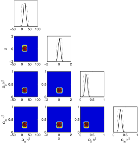
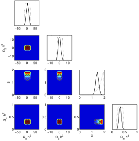
The mode of joined posterior pdf as well as mean (together with $68\%$ credible interval) of marginalized posterior pdf were calculated, by means of Markov Chains Monte Carlo analysis, using free accessible CosmoNest code Mukherjee et al. (2006) which has been modified for our purpose. The results are presented on fig. 2,3.

The numerical values of best fitted parameters for two our models as well as for $\Lambda$CDM are collected in table 1: the previous estimations without the GRB data (i.e. SNIa, H(z) and BAO and CMB) are shown in top part of the table. The new estimations including the GRB data occupy bottom part of the table.

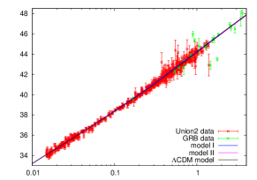
Quality of the estimation can be visualized on the Hubble’s diagram (fig. 1). Both of our models are in good agreement in the observational data.

Figure 1: Comparison of Hubble’s diagrams for models: I (blue), II (magenta) and $\Lambda$CDM (black).

Figure 2: Constraints of the parameters of model $I$. In 2D plots solid lines are the 68% and 95% confidence intervals from the marginalized probabilities. The colors describe the mean likelihood of the sample. In 1D plots solid lines denote marginalized probabilities of the sample, dotted lines are mean likelihood. For numerical results see Table 1.

Figure 3: Constraints of the parameters of model $II$. The meaning of the colors and the lines this same as in the picture 2. For numerical results see Table 1.

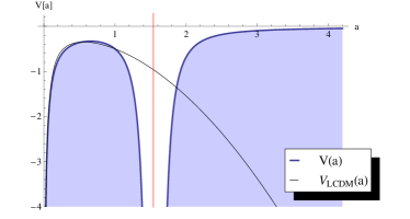
Figure 4: The diagram of the effective potential in particle–like representation of cosmic dynamics for model I versus $\Lambda$CDM model. Note that till the present epoch two potential plots almost coincide. Particulary, one can observe decelerating BB era. Maximum of the potential function corresponds to Einstein’s unstable static solution. Discrepancies become important in the future time: e.g. discontinuities of the potential functions (vertical, red line) denote that $V\rightarrow-\infty$, i.e. $\dot{a}\rightarrow\infty$ for $a\rightarrow a^{final}$. It turns out to be finite–time (sudden) singularity. In any case the shadowed region below the graph is forbidden for the motion.

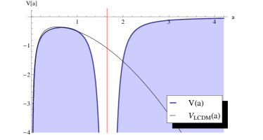
Figure 5: The diagram of the effective potential in particle like representation of cosmic dynamics for the model $II_{\alpha=0}$ versus $\Lambda$CDM model. Maximum of the potential function corresponds to unstable static solution. Again, until the present epoch there is no striking differences between plots. One can observe finite–size sudden singularity in the near future (vertical, red line). In any case the shadowed region below the potential is forbidden for the motion.

3 Conclusions

In this paper we continued and completed analysis of new cosmological models which were previously described and investigated in our paper Borowiec et al. (2011). Adding GRB data Tsutsui et al. (2012) allowed us to obtain better constraints of parameter $\Omega_{\alpha}$ which wasn’t present previously.

As it can be seen on the potential plots (fig. 4,5, both models dynamically mimics $\Lambda$CDM model from the Big Bang singularity until the present time. Discrepancies will appear in the near future. Both of our models predict the final finite size and finite time singularities (at $a=1.673$ for the model I, and at $a=1.559$ for the model II). However, comparing with our previous simulations, adding new GRB data has changed properties of the model II (Big Bounce is now replaced by Big Bang).

models I - the parameters estimated without GRB data
$\Omega_{0,\alpha}$	$\Omega_{0,\beta}$	$\delta$	$\Omega_{0,m}$
$-18.031^{+3.911}_{-11.969}(-6.210)$	$5.678^{+4.322}_{-1.489}(2.190)$	$0.238^{+0.075}_{-0.010}(0.229)$	$0.25\pm 0.03(0.23)$
models II - the parameters estimated without GRB data
$\Omega_{0,\alpha}$	$\Omega_{0,c}$	$\delta$	$\Omega_{0,\beta}$	$\Omega_{0,m}$
$-44.686^{+5.016}_{-15.314}(-57.870)$	$0.715^{+0.196}_{-0.393}(0.232)$	$0.598^{+0.008}_{-0.011}(0.560)$	$0.009\pm 0.005(0.003)$	$0.05^{+0.05}_{-0.04}(0.001)$
model $\Lambda$CDM - the parameter estimated without GRB data
$0.262^{+0.011}_{-0.012}(0.262)$
models I - the parameters estimated using GRB data
$\Omega_{0,\alpha}$	$\Omega_{0,\beta}$	$\delta$	$\Omega_{0,m}$
$3.809^{+0.133}_{-0.150}(3.776)$	$0.0002^{+0.023}_{-0.0002}(0.011)$	$1.605^{+0.083}_{-0.275}(1.413)$	$0.315^{+0.013}_{-0.014}(0.316)$
models II - the parameters estimated using GRB data
$\Omega_{0,\alpha}$	$\Omega_{0,c}$	$\delta$	$\Omega_{0,\beta}$	$\Omega_{0,m}$
$17.754^{+1.041}_{-0.840}(17.829)$	$1.157^{+0.044}_{-0.020}(1.163)$	$0.069^{+0.015}_{-0.012}(0.071)$	$0.254^{+0.008}_{-0.011}(0.253)$	$0.293^{+0.015}_{-0.012}(0.295)$
model $\Lambda$CDM - the parameter estimated using GRB data
$0.260^{+0.004}_{-0.003}(0.260)$

Table 1: The values of estimated parameters (mean of the marginalized posterior probabilities and $68\%$ credible intervals or sample square roots of variance, together with mode of the joined posterior probabilities, shown in brackets) for two investigated models. We compare estimations without GRB data (top part of the table) with the one employing GRB data (bottom part).

References

• Borowiec et al. (2011) A. Borowiec, M. Kamionka, A. Kurek and M. Szydlowski, “Cosmic acceleration from modified gravity with Palatini formalism,” JCAP 1202, 027 (2012), arXiv:1109.3420.
• Tsutsui et al. (2012) R. Tsutsui, T. Nakamura, D. Yonetoku, K. Takahashi and Y. Morihara, “Gamma-Ray Bursts are precise distance indicators similar to Type Ia Supernovae?”,(2012), arXiv:1205.2954.
• Amanullah et al. (2010) R. Amanullah et al., “Spectra and Light Curves of Six Type Ia Supernovae at 0.511 ¡ z ¡ 1.12 and the Union2 Compilation”, Astrophys. J.  716, 712 (2010), arXiv:1004.1711.
• Simon et al. (2004) J. Simon, L. Verde, R. Jimenez, “Constraints on the redshift dependence of the dark energy potential”, Phys. Rev.  D71, 123001 (2005), astro-ph/0412269.
• Eisenstein et al. (2005) D. J. Eisenstein et al., “Detection of the baryon acoustic peak in the large-scale correlation function of SDSS luminous red galaxies”, Astrophys. J.  633, 560-574 (2005), astro-ph/0501171;
W. J. Percival, S. Cole, D. J. Eisenstein, R. C. Nichol, J. A. Peacock, A. C. Pope, A. S. Szalay, “Measuring the Baryon Acoustic Oscillation scale using the SDSS and 2dFGRS”, Mon. Not. Roy. Astron. Soc.  381, 1053-1066 (2007), arXiv:0705.3323;
B. A. Reid et al., “Baryon Acoustic Oscillations in the Sloan Digital Sky Survey Data Release 7 Galaxy Sample”, Mon. Not. Roy. Astron. Soc.  401, 2148-2168 (2010), arXiv:0907.1660.
• Komatsu et al. (2010) E. Komatsu et al., “Seven-Year Wilkinson Microwave Anisotropy Probe (WMAP) Observations: Cosmological Interpretation”, Astrophys. J. Suppl.  192, 18 (2011), arXiv:1001.4538.
• Bond et al. (1997) J. R. Bond, G. Efstathiou, M. Tegmark, “Forecasting cosmic parameter errors from microwave background anisotropy experiments”, Mon. Not. Roy. Astron. Soc.  291, L33-L41 (1997), astro-ph/9702100.
• Riess et al. (2009) A. G. Riess et al., “A Redetermination of the Hubble Constant with the Hubble Space Telescope from a Differential Distance Ladder”, Astrophys. J.  699, 539 (2009), arXiv:0905.0695.
• Mukherjee et al. (2006) P. Mukherjee, D. Parkinson, A. R. Liddle, “A nested sampling algorithm for cosmological model selection”, Astrophys. J.  638, L51-L54 (2006), astro-ph/0508461;
P. Mukherjee, D. Parkinson, P. S. Corasaniti, A. R. Liddle, M. Kunz, “Model selection as a science driver for dark energy surveys”, Mon. Not. Roy. Astron. Soc.  369, 1725-1734 (2006), astro-ph/0512484;
D. Parkinson, P. Mukherjee, A.R. Liddle, “A Bayesian model selection analysis of WMAP3”, Phys. Rev.  D73, 123523 (2006), astro-ph/0605003;
http://cosmonest.org/