DESY 13-038                                                                                                                                            HU-EP-13/08                                                                                                                                         SFB-CPP-13-17 Chiral condensate from the twisted mass Dirac operator spectrum

Abstract

We present the results of our computation of the dimensionless chiral condensate $r_{0}\Sigma^{1/3}$ with $N_{f}=2$ and $N_{f}=2+1+1$ flavours of maximally twisted mass fermions. The condensate is determined from the Dirac operator spectrum, applying the spectral projector method proposed by Giusti and Lüscher. We use 3 lattice spacings and several quark masses at each lattice spacing to perform the chiral and continuum extrapolations. We study the effect of the dynamical strange and charm quarks by comparing our results for $N_{f}=2$ and $N_{f}=2+1+1$ dynamical flavours.

1 Introduction

One of the most important phenomena of QCD is the spontaneous breaking of chiral symmetry. This purely non-perturbative phenomenon was subject to many analyses in Lattice QCD, using different fermion discretizations and methods. In particular, the chiral condensate – the order parameter of spontaneous chiral symmetry breaking – can be extracted from chiral perturbation theory fits of the quark-mass dependence of light pseudoscalar meson observables Aoki:2008sm ; Allton:2008pn ; Aoki:2010dy ; Bazavov:2009bb ; Bazavov:2010yq ; Baron:2009wt ; Fukaya:2010na ; Bernard:2012fw ; Borsanyi:2012zv , the topological susceptibility Durr:2001ty ; Chiu:2008jq ; Chiu:2011dz ; Bernardoni:2010nf ; Bernard:2012fw or the pion electromagnetic form factor Frezzotti:2008dr . Other methods include using the $\epsilon$-regime expansion and/or chiral random matrix theory Hernandez:1999cu ; Damgaard:2000qt ; DeGrand:2005vb ; Lang:2006ab ; Fukaya:2007fb ; Fukaya:2007yv ; Fukaya:2010na ; Hasenfratz:2008ce ; Jansen:2009tt ; Bernardoni:2010nf ; Splittorff:2012gp , Wilson chiral perturbation theory fits of the integrated spectral density Necco:2011vx ; Necco:2011jz ; Necco:2013sxa and a calculation directly from the quark propagator Burger:2012ti ; McNeile:2012xh . A summary of recent results is provided in Ref. Colangelo:2010et .

The chiral condensate is related to the spectral density of the Dirac operator via the Banks-Casher relation Banks:1979yr :

$$\lim_{\lambda\rightarrow 0}\lim_{m\rightarrow 0}\lim_{V\rightarrow\infty}\rho(\lambda,m)=\frac{\Sigma}{\pi},$$ (1)

where $\lambda$ is the modulus of the eigenvalue, $m$ the quark mass, $\rho(\lambda,m)$ the spectral density, $V$ the volume and $\Sigma$ is the chiral condensate in the infinite-volume and in the chiral limit. Clearly, the triple limit on the left-hand side of the above equation makes it impractical to evaluate the chiral condensate on the lattice.

However, recently a method has been proposed Giusti:2008vb to effectively make use of the Banks-Casher relation and explore the chiral properties of QCD on the lattice, in particular to compute the chiral condensate. The method has also other applications, e.g. it allows to compute the topological susceptibility or renormalization constants. Briefly, the method consists in stochastically evaluating the mode number, i.e. the number of eigenmodes of the Dirac operator below some spectral threshold value and using the dependence of this number of eigenmodes on the threshold value to calculate the observable of interest. In the following, we will refer to this method as spectral projectors. One of its essential advantages for computing the mode number is the fact that it is very effective in terms of computational cost – the required computational effort grows linearly with the lattice volume instead of quadratically, as is the case for a direct computation of eigenmodes and counting their number below the spectral threshold.

In this paper, we report our results for the chiral condensate with $N_{f}=2$ and $N_{f}=2+1+1$ Wilson twisted mass fermions at maximal twist. Preliminary results of our computations for the $N_{f}=2+1+1$ case were presented in Ref. Cichy:2011an . The paper is organized as follows. In the second section we provide a short description of the spectral projector method. In section 3, we describe our lattice setup. Section 4 presents our results for the chiral condensate both in the $N_{f}=2$ and the $N_{f}=2+1+1$ case. In section 5, we summarize and compare with other determinations of the chiral condensate found in literature. An appendix presents our tests of the method.

2 Spectral projectors and chiral condensate

Many interesting properties of the chiral regime of QCD can be understood from the behaviour of quantities related to the low-lying spectrum of the Dirac operator. One of such spectral quantities, essential in the determination of the chiral condensate, is the mode number, i.e. the number of eigenvectors of the massive Hermitian Dirac operator $D^{\dagger}D$ with eigenvalue magnitude smaller than some threshold value $M^{2}$. We will denote this mode number by $\nu(M,\mu)$, where $\mu$ is the quark mass.

Here we provide a short description of the spectral projector method for the computation of $\nu(M,\mu)$. For a more complete exposition, we refer to the original work of Ref. Giusti:2008vb . In this section we assume that we work on an Euclidean lattice, but we will not specify the particular form of the lattice Dirac operator.

If $\mathbbm{P}_{M}$ is the orthogonal projector to the subspace of fermion fields spanned by the lowest lying eigenmodes of the massive Hermitian Dirac operator $D^{\dagger}D$ with eigenvalues below some threshold value $M^{2}$, the mode number $\nu(M,\mu)$ can be represented stochastically by:

$$\nu(M,\mu)=\langle\textrm{Tr}\,\mathbbm{P}_{M}\rangle=\left\langle\frac{1}{N}\sum_{j=1}^{N}(\eta_{j},\mathbbm{P}_{M}\eta_{j})\right\rangle,$$ (2)

where $\eta_{1}$, $\ldots$, $\eta_{N}$ are pseudo-fermion fields added to the theory.

The orthogonal projector $\mathbbm{P}_{M}$ can be approximated by a rational function of $D^{\dagger}D$:

$$\mathbbm{P}_{M}\approx h(\mathbbm{X})^{4},\qquad\mathbbm{X}=1-\frac{2M_{*}^{2}}{D^{\dagger}D+M_{*}^{2}},$$ (3)

where $M_{*}$ is a mass parameter related to the spectral threshold value $M$. The function:

$$h(x)=\frac{1}{2}\left(1-xP(x^{2})\right)$$ (4)

is an approximation to the step function $\theta(-x)$ in the range $-1\leq x\leq 1$, where $P(y)$ is in our case the Chebyshev polynomial (of some adjustable degree $n$) that minimizes the deviation:

$$\delta=\max_{\epsilon\leq y\leq 1}|1-\sqrt{y}P(y)|$$ (5)

for some $\epsilon>0$. Computing the approximation to the spectral projector $\mathbbm{P}_{M}$ requires solving the following equation an appropriate number of times:

$$(D^{\dagger}D+M_{*}^{2})\psi=\eta$$ (6)

for a given source field $\eta$. Solving this equation is the main computational cost in the calculation of the mode number. In particular, the computational cost scales linearly $V$ with the volume.

One can show Giusti:2008vb that the mode number is a renormalization group invariant, i.e.:

$$\nu_{R}(M_{R},\mu_{R})=\nu(M,\mu),$$ (7)

where the subscript $R$ denotes renormalized quantities. Note that the spectral threshold parameter $M$ renormalizes in the same way as the light quark mass (i.e. $M_{R}=Z_{P}^{-1}M$ for Wilson twisted mass fermions).

Finally, we give here the relation between the mode number and the mass-dependent renormalized chiral condensate: Giusti:2008vb

$$\Sigma_{R}=\frac{\pi}{2V}\sqrt{1-\left(\frac{\mu_{R}}{M_{R}}\right)^{2}}\frac{\partial}{\partial M_{R}}\nu_{R}(M_{R},\mu_{R}),$$ (8)

which is defined to match the chiral condensate to leading order of chiral perturbation theory.

3 Lattice setup

In this section, we will specify the lattice Dirac operator that is used for our work, i.e. the Wilson twisted mass Dirac operator. For our computations of the chiral condensate, we have used gauge field configurations generated by the European Twisted Mass Collaboration (ETMC) with $N_{f}=2$ Boucaud:2007uk ; Boucaud:2008xu ; Baron:2009wt and $N_{f}=2+1+1$ Baron:2010bv ; Baron:2010th ; Baron:2011sf dynamical quarks.

The gauge action is:

$$S_{G}[U]=\frac{\beta}{3}\sum_{x}\Big{(}b_{0}\sum_{\mu,\nu=1}\textrm{Re\,Tr}\big{(}1-P^{1\times 1}_{x;\mu,\nu}\big{)}+b_{1}\sum_{\mu\neq\nu}\textrm{Re\,Tr}\big{(}1-P^{1\times 2}_{x;\mu,\nu}\big{)}\Big{)},$$ (9)

with $\beta=6/g_{0}^{2}$, $g_{0}$ the bare coupling and $P^{1\times 1}$, $P^{1\times 2}$ are the plaquette and rectangular Wilson loops, respectively. For the $N_{f}=2$ case, we use the tree-level Symanzik improved action Weisz:1982zw , i.e. we set $b_{1}=-\frac{1}{12}$, with the normalization condition $b_{0}=1-8b_{1}$. In the case of $N_{f}=2+1+1$, we use the Iwasaki action Iwasaki:1985we ; Iwasaki:1996sn , i.e. $b_{1}=-0.331$.

The Wilson twisted mass fermion action for the light, up and down quarks for both the $N_{f}=2$ and $N_{f}=2+1+1$ cases, is given in the so-called twisted basis by: Frezzotti:2000nk ; Frezzotti:2003ni ; Frezzotti:2004wz ; Shindler:2007vp

$$S_{l}[\psi,\bar{\psi},U]=a^{4}\sum_{x}\bar{\chi}_{l}(x)\big{(}D_{W}+m_{0,l}+i\mu_{l}\gamma_{5}\tau_{3}\big{)}\chi_{l}(x),$$ (10)

where $m_{0,l}$ and $\mu_{l}$ denote, respectively, the bare untwisted and twisted light quark masses (for shortness, whenever there is no risk of confusion, from now on we will use the symbol $\mu$ to denote $\mu_{l}$). The renormalized light quark mass is given by $\mu_{R}=Z_{P}^{-1}\mu$. The matrix $\tau^{3}$ acts in flavour space and $\chi_{l}=(\chi_{u},\,\chi_{d})$ is a two-component vector in flavour space, related to the one in the physical basis by a chiral rotation. The standard massless Wilson-Dirac operator $D_{W}$ reads:

$$D_{W}=\frac{1}{2}\big{(}\gamma_{\mu}(\nabla_{\mu}+\nabla^{*}_{\mu})-a\nabla^{*}_{\mu}\nabla_{\mu}\big{)},$$ (11)

where $\nabla_{\mu}$ and $\nabla^{*}_{\mu}$ are the forward and backward covariant derivatives.

The twisted mass action for the heavy doublet is given by: Frezzotti:2004wz ; Frezzotti:2003xj

$$S_{h}[\psi,\bar{\psi},U]=a^{4}\sum_{x}\bar{\chi}_{h}(x)\big{(}D_{W}+m_{0,h}+i\mu_{\sigma}\gamma_{5}\tau_{1}+\mu_{\delta}\tau_{3}\big{)}\chi_{h}(x),$$ (12)

where $m_{0,h}$ denotes the bare untwisted heavy quark mass, $\mu_{\sigma}$ the bare twisted mass with the twist along the $\tau_{1}$ direction and $\mu_{\delta}$ the mass splitting along the $\tau_{3}$ direction, introduced to make the strange and charm quark masses non-degenerate. The mass parameters $\mu_{\sigma}$ and $\mu_{\delta}$ are related to the physical renormalized strange $m^{s}_{R}$ and charm $m^{c}_{R}$ quark masses by $m^{s,c}_{R}=Z_{P}^{-1}\left(\mu_{\sigma}\mp(Z_{P}/Z_{S})\mu_{\delta}\right)$. The heavy quark doublet in the twisted basis $\chi_{h}=(\chi_{c},\,\chi_{s})$ is again related to the one in the physical basis by a chiral rotation.

Ensemble	$\beta$	lattice	$a\mu$	$\mu_{R}$ [MeV]	$\kappa_{c}$	$L$ [fm]
b$30.32$	3.90	$32^{3}\times 64$	0.003	16	0.160856	2.7
b$40.16$	3.90	$16^{3}\times 32$	0.004	21	0.160856	1.4
b$40.20$	3.90	$20^{3}\times 40$	0.004	21	0.160856	1.7
b$40.24$	3.90	$24^{3}\times 48$	0.004	21	0.160856	2.0
b$40.32$	3.90	$32^{3}\times 64$	0.004	21	0.160856	2.7
b$64.24$	3.90	$24^{3}\times 48$	0.0064	34	0.160856	2.0
b$85.24$	3.90	$24^{3}\times 48$	0.0085	45	0.160856	2.0
c$30.32$	4.05	$32^{3}\times 64$	0.003	19	0.157010	2.1
c$60.32$	4.05	$32^{3}\times 64$	0.006	37	0.157010	2.1
c$80.32$	4.05	$32^{3}\times 64$	0.008	49	0.157010	2.1
d$20.48$	4.20	$48^{3}\times 96$	0.002	15	0.154073	2.6
d$65.32$	4.20	$32^{3}\times 64$	0.0065	47	0.154073	1.7

Table 1: Parameters of the $N_{f}=2$ gauge ensembles Boucaud:2007uk ; Boucaud:2008xu ; Baron:2009wt . We show the inverse bare coupling $\beta$, lattice size $(L/a)^{3}\times(T/a)$, bare twisted light quark mass $a\mu$, renormalized quark mass $\mu_{R}$ in MeV, critical value of the hopping parameter at which the PCAC mass vanishes and physical extent of the lattice $L$ in fm.

The twisted mass formulation allows for an automatic $\mathcal{O}(a)$ improvement of physical observables, provided the hopping parameter $\kappa=(8+2am_{0})^{-1}$, where $m_{0}\equiv m_{0,l}=m_{0,h}$ can be chosen, is tuned to maximal twist by setting it to its critical value, at which the PCAC quark mass vanishes Frezzotti:2003ni ; Chiarappa:2006ae ; Farchioni:2004ma ; Farchioni:2004fs ; Frezzotti:2005gi ; Jansen:2005kk .

Ensemble	$\beta$	lattice	$a\mu_{l}$	$\mu_{l,R}$ [MeV]	$\kappa_{c}$	L [fm]
A30.32	1.90	$32^{3}\times 64$	0.0030	13	0.163272	2.8
A40.20	1.90	$20^{3}\times 40$	0.0040	17	0.163270	1.7
A40.24	1.90	$24^{3}\times 48$	0.0040	17	0.163270	2.1
A40.32	1.90	$32^{3}\times 64$	0.0040	17	0.163270	2.8
A50.32	1.90	$32^{3}\times 64$	0.0050	22	0.163267	2.8
A60.24	1.90	$24^{3}\times 48$	0.0060	26	0.163265	2.1
A80.24	1.90	$24^{3}\times 48$	0.0080	35	0.163260	2.1
B25.32	1.95	$32^{3}\times 64$	0.0025	13	0.161240	2.5
B35.32	1.95	$32^{3}\times 64$	0.0035	18	0.161240	2.5
B55.32	1.95	$32^{3}\times 64$	0.0055	28	0.161236	2.5
B75.32	1.95	$32^{3}\times 64$	0.0075	38	0.161232	2.5
B85.24	1.95	$24^{3}\times 48$	0.0085	45	0.161231	1.9
D15.48	2.10	$48^{3}\times 96$	0.0015	9	0.156361	2.9
D20.48	2.10	$48^{3}\times 96$	0.0020	12	0.156357	2.9
D30.48	2.10	$48^{3}\times 96$	0.0030	19	0.156355	2.9

Table 2: Parameters of the $N_{f}=2+1+1$ gauge ensembles Baron:2010bv ; Baron:2010th ; Baron:2011sf . We show the inverse bare coupling $\beta$, lattice size $(L/a)^{3}\times(T/a)$, bare twisted light quark mass $\mu_{l}$, renormalized quark mass $\mu_{l,R}$ in MeV, critical value of the hopping parameter at which the PCAC mass vanishes and physical extent of the lattice $L$ in fm.

$N_{f}$	$\beta$	$a$ [fm]	$Z_{P}(\overline{\textrm{MS}},\,2\,{\rm GeV})$	$r_{0}/a$
2	3.90	0.085	0.437(7)	5.35(4)
2	4.05	0.067	0.477(6)	6.71(4)
2	4.20	0.054	0.501(13)	8.36(6)
2+1+1	1.90	0.0863	0.529(9)	5.231(38)
2+1+1	1.95	0.0779	0.504(5)	5.710(41)
2+1+1	2.10	0.0607	0.514(3)	7.538(58)

Table 3: The values of the lattice spacing $a$ Blossier:2010cr ; Baron:2011sf , $r_{0}/a$ Blossier:2010cr ; Baron:2010bv ; Ottnad:2012fv and the renormalization constant $Z_{P}$ in the $\overline{\textrm{MS}}$ scheme at the scale of 2 GeV Constantinou:2010gr ; Alexandrou:2012mt ; Palao:priv , for different values of $\beta$ and $N_{f}=2$ and $N_{f}=2+1+1$.

The details of the ensembles considered for this work are presented in Tab. 1 for $N_{f}=2$ and Tab. 2 for $N_{f}=2+1+1$. For both cases, they include 3 lattice spacings (from $a\approx 0.05$ to $a\approx 0.085$ fm) and up to 5 quark masses at a given lattice spacing. The renormalized light quark masses $\mu_{R}$ are in the range from around 15 to 50 MeV. The values of the renormalization constant $Z_{P}$ for different ensembles Constantinou:2010gr ; Alexandrou:2012mt ; Palao:priv , used to convert bare light quark masses $\mu$ and bare spectral threshold parameters $M$ to their renormalized values in the $\overline{\textrm{MS}}$ scheme (at the scale of 2 GeV), are given in Tab. 3, where we also show the values of $r_{0}/a$ (in the chiral limit), used to express our results for the condensate as a dimensionless product $r_{0}\Sigma^{1/3}$. Our physical lattice extents $L$ for extracting physical results range from 2 to 3 fm (in the temporal direction, we always have $T=2L$). To check for the size of finite volume effects, we included different lattice sizes for $\beta=3.9$, $a\mu=0.004$ ($N_{f}=2$) and $\beta=1.9$, $a\mu=0.004$ ($N_{f}=2+1+1$).

4 Results

In this section, we show our results of the calculation of the chiral condensate. First, we illustrate the procedure of extraction of the chiral condensate and discuss the influence of the various errors that enter the computation. Then, we analyze finite volume effects in our simulations. Finally, we move on to our chiral and continuum extrapolations.

4.1 Procedure and errors

We show here how to extract the mass-dependent chiral condensate according to Eq. (8), illustrating the procedure for ensemble B40.32. Using the spectral projector method, we computed the dependence of the mode number on the renormalized spectral threshold parameter $M_{R}$ for 5 values of $M_{R}$, from around 2.5 times the renormalized quark mass to around 120 MeV. Shortly above the latter value one starts to see deviations from the linear regime of $\nu_{R}(M_{R},\mu_{R})$ vs. $M_{R}$ (see Appendix A).

Fig. 1 shows the dependence of the mode number on the renormalized spectral threshold parameter $M_{R}$. The solid line is a linear fit to all 5 points. The slope of this line $\partial\nu_{R}(M_{R},\mu_{R})/\partial M_{R}$ determines the value of the mass-dependent chiral condensate according to Eq. (8). The error of this slope includes two sources: the error of the slope of the bare mode number as function of the bare threshold parameter $M$, $\partial\nu(M,\mu)/\partial M$ and the error of $Z_{P}$ needed to convert from bare to renormalized quantities. Although $\partial\nu_{R}(M_{R},\mu_{R})/\partial M_{R}$ appears to be constant as a function of $M_{R}$ within errors, we will take its value to be the middle point of the chosen fitting interval, see below for details of the fitting intervals considered. Finally, Eq. (8) yields, after taking the cubic root:

$$a\Sigma^{1/3}=0.13372(34)(72),$$

where the first error is the one of the slope $\partial\nu(M,\mu)/\partial M$ and the other one comes from $Z_{P}=0.437(7)$ and is dominated by systematic effects – hence, we take it as a systematic error of our computation.

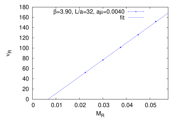
Figure 1: Dependence of the mode number on the renormalized spectral threshold parameter $M_{R}$ for ensemble B40.32. The solid line is a linear fit to all 5 points.

fit range	lowest $aM_{R}$	highest $aM_{R}$	$\chi^{2}/{\rm dof}$	$r_{0}\Sigma^{1/3}$
1 – 3	0.0225	0.0375	0.004	0.7085(43)
1 – 4	0.0225	0.0450	0.018	0.7116(24)
1 – 5	0.0225	0.0525	0.588	0.7154(18)
2 – 4	0.0300	0.0450	0.006	0.7141(46)
2 – 5	0.0300	0.0525	0.567	0.7189(33)
3 – 5	0.0375	0.0525	0.549	0.7235(57)

Table 4: Values of $r_{0}\Sigma^{1/3}$ extracted from different fitting ranges. Every fit includes at least 3 values of $M_{R}$. The fit labeled “1 – 5” is the full fit. We estimate the error from the choice of the fitting range by comparing the value from the full fit with the ones from fits “1 – 4” and “2 – 5”. The error given is statistical only.

The value of $a\Sigma^{1/3}$ can be further converted to a dimensionless product $r_{0}\Sigma^{1/3}$ (which will be the final result of this paper, after taking the chiral and continuum limits) or to a physical value in MeV. For the former, we use the value in the chiral limit $r_{0}/a=5.35(4)$. Since the error of this value is again mostly systematic, we quote it as another systematic error of $r_{0}\Sigma^{1/3}$:

$$r_{0}\Sigma^{1/3}=0.7154(18)(39)(53),$$

where the two errors are as above and the third one comes from $r_{0}/a$. For a conversion to MeV, one needs to choose a value of the lattice spacing in physical units. There are several such estimates for ETMC 2-flavour ensembles, giving for $\beta=3.9$ values including 0.079 fm Baron:2009wt , 0.085 fm Blossier:2010cr and 0.089 fm Alexandrou:2008tn . Taking this spread into account, the relative error on the lattice spacing is around 7%, which leads to a similar relative uncertainty in the value of the chiral condensate $\Sigma^{1/3}$ in physical units, which amounts to about 20 MeV. This is roughly an order of magnitude more than other errors entering our computation. Even being less conservative and using for the error the value quoted in Ref. Blossier:2010cr – 0.085(2)_stat(1)_syst fm – the error that it yields is still of the order of 10 MeV. Therefore, we decided to give our final results as the dimensionless product $r_{0}\Sigma^{1/3}$ and we chose not to quote any value in MeV for it until a significantly improved determination of the lattice spacing is available.

Another source of the error is the choice of the fitting range and hence the value of $M_{R}$ that enters the square root in Eq. (8). Of course, physical results should not depend on this choice, provided that the whole fitting interval lies in the linear regime of the mode number vs. $M_{R}$ dependence. Hence, varying the fitting range serves two purposes: establishing whether non-linear effects are already present and checking that the choice of $M_{R}$ in Eq. (8) does not influence the final result. The values of $r_{0}\Sigma^{1/3}$ resulting from different fitting ranges in $M_{R}$ are shown in Tab. 4. For all fits, $\chi^{2}/{\rm d.o.f.}$ is below 1. The compatibility of all results and the good values of $\chi^{2}/{\rm d.o.f.}$ imply that for this ensemble the choice of the fitting range and $M_{R}$ does not affect the results in a substantial way. To quantify this error, we considered the 4-point fits with the lowest or highest value of $M_{R}$ excluded. Excluding the first or last point leads to a similar change of the result and hence we took the larger of the two as our conservative error from the choice of the fitting range. Note, however, that Tab. 4 implies a systematic tendency towards increasing of $\Sigma$ when the fitting range moves towards higher values of $M_{R}$. This indicates an onset of non-linear behaviour for values of $M_{R}$ only slightly above the ones we considered.

Finally, our estimate of $r_{0}\Sigma^{1/3}$ for ensemble B40.32, including all sources of error, is:

$$r_{0}\Sigma^{1/3}=0.7154(18)_{\rm stat}(38)_{\rm fit}\,{}_{\rm range}(39)_{Z_{P}}(53)_{r_{0}/a}.$$

We note that the total error is dominated by systematic errors. This means that increasing statistics would not essentially change our total error. It should be considered an important advantage of the method of spectral projectors that rather moderate statistics (in our case around 230 independent gauge field configurations for this ensemble) leads to a practically negligible statistical error. Let us also mention that the quoted statistical error takes autocorrelations fully into account. We performed an analysis of autocorrelations using two methods and found that in general the autocorrelations are small, even at our smallest lattice spacings. For the details of our autocorrelation analysis, we refer to Appendix B.

4.2 Finite volume effects

One of the main sources of systematic effects in Lattice QCD simulations are finite volume effects (FVE). In Ref. Giusti:2008vb , theoretical arguments were provided that FVE should be small for the chiral condensate computed from the mode number – with exponentially small difference between the finite volume and infinite volume results of $\mathcal{O}(\exp(-M_{\Lambda}L/2))$, where $M_{\Lambda}^{2}=2\Lambda\Sigma/F^{2}$, $\Lambda=\sqrt{M^{2}-\mu^{2}}$ and $F$ is the pion decay constant in the chiral limit. Since in practice the mass-dependent chiral condensate is extracted at $\Lambda\gg\mu$, the mass $M_{\Lambda}$ is much higher than the pion mass, which typically governs FVE. Hence, one expects that for the computation of the chiral condensate from the mode number, FVE will be rather small. FVE for the mode number itself were computed in SU(2) chiral perturbation theory Necco:2011vx . The resulting formula leads to a prediction that FVE from lattices with $L\geq 2$ fm should be small, $\mathcal{O}(\lesssim 1\%)$ for $M_{R}\approx\mathcal{O}(60-120)$ MeV and renormalized quark masses of $\mathcal{O}(10-20)$ MeV (with larger FVE at smaller $M_{R}$). Indeed, in practice, it was shown in Ref. Giusti:2008vb that for $L\geq 2$ fm the results deviate from their infinite volume values by less than 1%.

To show that it is also the case in our setup, we performed the computation of the mode number and the chiral condensate for:

• $N_{f}=2:\;$ 4 different volumes at fixed $\beta=3.9$, $a\mu=0.004$, lattice extents: $L/a=16$, 20, 24 and 32, with corresponding physical values of 1.4, 1.7, 2.0 and 2.7 fm, respectively,

• $N_{f}=2+1+1:\;$ 3 different volumes at fixed $\beta=1.9$, $a\mu=0.004$, lattice extents: $L/a=20$, 24 and 32, with corresponding physical values of 1.7, 2.1 and 2.8 fm, respectively.

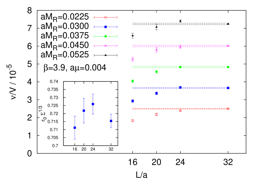
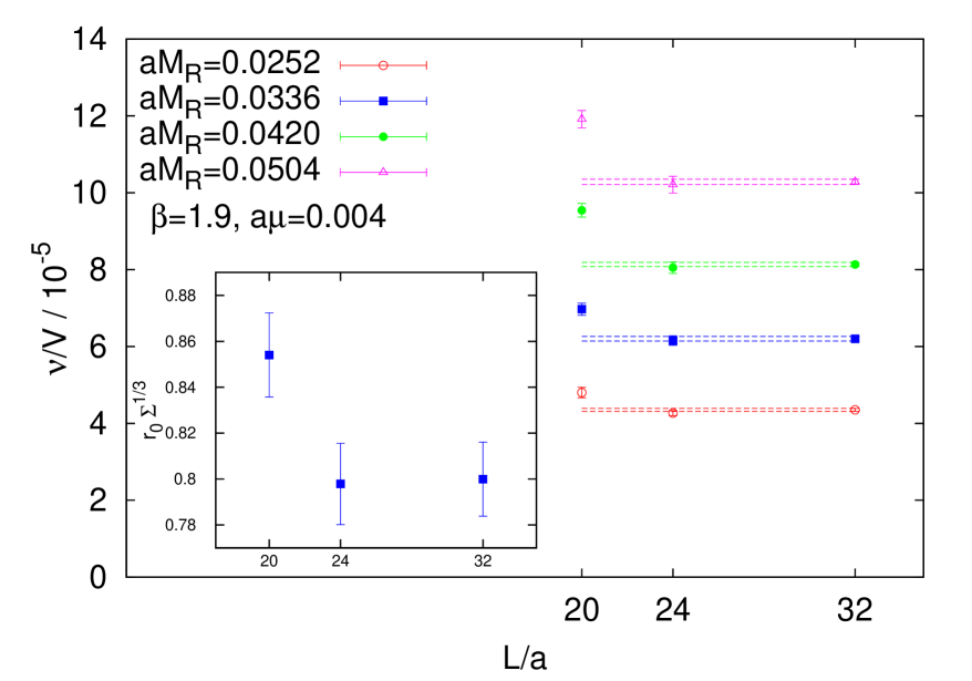
Figure 2: The main plots show the volume dependence of the mode number density $\nu/V$ for different values of the renormalized spectral threshold $M_{R}$. The horizontal bands show the result at the largest volume. The insets show the volume dependence of the chiral condensate $r_{0}\Sigma^{1/3}$ (the error of each point includes the statistical error and the systematic one originating from the choice of the fitting interval). (Left) $N_{f}=2$, $\beta=3.9$, $a\mu=0.004$, (right) $N_{f}=2+1+1$, $\beta=1.9$, $a\mu=0.004$.

In Fig. 2, we show the volume dependence of the mode number density $\nu/V$ for 4-5 different values of the renormalized spectral threshold $M_{R}$. The mode number density can be computed very precisely. It hence provides a strong test of finite size effects.

The left plot shows our data for $N_{f}=2$. The results for $L/a=20$ and especially $L/a=16$ are systematically lower than $L/a=32$, signaling large FVE. However, the mode number density for $L/a=24$ is compatible with the one for $L/a=32$ for 3 intermediate values of $M_{R}$, while it differs by 2-3$\sigma$ for the lowest and highest $M_{R}$, thus changing the slope of the mode number vs. $M_{R}$ dependence and the extracted chiral condensate (see the inset of Fig. 2 (left)). This change of slope is statistically significant, but it is still a relatively small, 1-1.5% effect. Taking into account the uncertainty from the choice of the fitting range, the final results for the chiral condensate are compatible for all cases – including the ones for small volumes, indicating that even if the mode number density goes systematically down, the slope of the whole $\nu(M_{R},\mu_{R})$ dependence is less affected. We have also tried a description of FVE in the framework of the formula derived in Ref. Necco:2011vx . We conclude that it provides a reasonable agreement with actual lattice data for $L/a\gtrsim 24$, while FVE for smaller volumes are somewhat underestimated (by a factor of $\mathcal{O}(2)$ at $L/a=16$, compared to the actually observed FVE).

In the right plot, we show analogous data for $N_{f}=2+1+1$. Similarly, we observe significant finite size effects in the mode number density (and also in the chiral condensate) for $L/a=20$, while $L/a=24$ and $L/a=32$ are always compatible.

This allows us to conclude that finite size effects are indeed very small when one reaches a linear lattice extent of around 2 fm ($L/a=24$ at both $\beta=3.9$ ($N_{f}=2$) and $\beta=1.9$ ($N_{f}=2+1+1$)). Therefore, we used in our analysis all available ETMC ensembles with a linear lattice extent of at least 2 fm.

4.3 Chiral and Continuum Limit – $N_{f}=2$

We now show our results for the 2-flavour case. For each value of $\beta$, we have 2-4 sea quark masses, according to Tab. 1. For each ensemble, we perform computations of the mode number at 5 values of the renormalized spectral threshold $M_{R}$, from around 50 to 120 MeV. We follow the procedure outlined in Sec. 4.1, i.e. we extract the mass-dependent condensate from the slope $\nu_{R}(M_{R},\mu_{R})$ as function of $M_{R}$ for each ensemble.

Ensemble	$a\mu$	$r_{0}\Sigma^{1/3}$
b$30.32$	0.0030	0.7118(29)(38)(53)
b$40.32$	0.0040	0.7154(18)(39)(53)
b$64.24$	0.0064	0.7246(26)(39)(54)
b$85.24$	0.0085	0.7377(23)(40)(55)
chiral		0.6957(35)(37)(52)(186)
c$30.32$	0.0030	0.7188(50)(30)(43)
c$60.32$	0.0060	0.7345(35)(30)(44)
c$80.32$	0.0080	0.7425(29)(31)(44)
chiral		0.7046(78)(30)(42)(206)
d$20.48$	0.0020	0.7036(45)(61)(51)
d$65.32$	0.0065	0.7415(40)(64)(53)
chiral		0.6853(73)(59)(49)(265)

Table 5: Results for $r_{0}\Sigma^{1/3}$ for all considered $N_{f}=2$ ensembles. The given errors are: statistical, resulting from $Z_{P}$, resulting from $r_{0}/a$, respectively. We also show results in the chiral limit, where we also give the systematic error from the choice of the fitting interval (4th error). See text for more details.

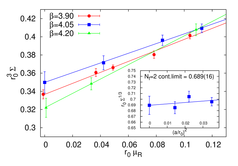
Figure 3: Main plot: chiral extrapolations of the chiral condensate $r_{0}^{3}\Sigma$ for $N_{f}=2$ ensembles and $\beta=3.9$, 4.05, 4.2. The lines are extrapolations to the chiral limit, linear in the quark mass. The values in the chiral limit for $\beta=3.9$ and 4.2 are slightly shifted for better presentation. The errors are statistical only. Inset: continuum extrapolation of the chirally extrapolated chiral condensate $r_{0}\Sigma^{1/3}$ vs. $(a/r_{0})^{2}$. The errors include: statistical errors, errors from $Z_{P}$ and errors from $r_{0}/a$.

The results for $r_{0}\Sigma^{1/3}$ for all considered ensembles are gathered in Tab. 5. These results are then used to extrapolate to the chiral limit for each value of $\beta$. The chiral corrections to the mass-dependent condensate were calculated at the next-to-leading order of chiral perturbation theory in Ref. Giusti:2008vb . The obtained formula suggests that the mass-dependent condensate is equal to the chiral condensate in the chiral limit up to terms linear in $\mu_{R}$ and higher order effects. In particular, there are no corrections proportional to $\mu_{R}\,\ln\mu_{R}$. Moreover, the size of these chiral corrections is small, as illustrated explicitly in Ref. Giusti:2008vb – inserting the values of low energy constants, it was shown that regardless of the value of $M_{R}$ at which the condensate is extracted, the curvature is very mild. Hence, in practice a linear extrapolation of the mass-dependent condensate to the chiral limit is fully justified and we follow this conclusion in our chiral extrapolations. As a check, we tried fits of the NLO formula (inserting values of the low energy constants used in Ref. Giusti:2008vb ) and we found that the differences with respect to the linear extrapolation are negligible compared to our errors.

Our extrapolations for all three values of $\beta$ are shown in the main plot of Fig. 3 (we plot $r_{0}^{3}\Sigma$ vs. $r_{0}\mu_{R}$ to allow comparisons between different values of $\beta$). The plotted errors are only statistical, since in extrapolations at fixed $\beta$, the relative errors from $Z_{P}$ and $r_{0}/a$ are the same for all quark mass values (we use chirally extrapolated values of $Z_{P}$ and $r_{0}/a$) – we give them in Tab. 5. To estimate the systematic error originating from the choice of the fitting range in $\nu_{R}(M_{R},\mu_{R})$ vs. $M_{R}$ fits, we repeated all chiral extrapolations for two tailored fitting ranges – excluding the first value of $M_{R}$ (to account for effects of coming too close to the renormalized quark mass) or the last value thereof (to account for possible deviations from the linear behaviour for too high values of $M_{R}$).

The chiral limit values, with all sources of error, are also shown in Tab. 5. In general, the total error originates in practice only from the choice of the fitting range and the latter increases when approaching the continuum limit. The reasons for this behaviour include the fact that the number of quark masses that we use decreases for smaller lattice spacings and at $\beta=4.2$ the slope of the quark mass dependence of the chiral condensate is apparently larger than at coarser lattice spacings, making the final chiral limit value more susceptible to changes in the fitting interval.

Finally, we can use the chirally extrapolated values of the condensate to perform an extrapolation to the continuum limit. We start by discussing the $\mathcal{O}(a)$-improvement of the chiral condensate. For on-shell quantities, $\mathcal{O}(a)$-improvement amounts to the quantity being even under the $\mathcal{R}_{5}$ parity transformation: $\psi\rightarrow i\gamma_{5}\tau^{1}\psi$, $\bar{\psi}\rightarrow i\bar{\psi}\gamma_{5}\tau^{1}$ Frezzotti:2003ni . Let us consider the spectral sums Giusti:2008vb : $\sigma_{k}(\mu,m_{q})=\langle\mathrm{Tr}\left\{(D_{m}^{\dagger}D_{m}+\mu^{2})^{-k}\right\}\rangle$, where $k\geq 3$ for reasons explained in the given reference. The spectral sums are related to the mode number Giusti:2008vb and the improvement (or lack thereof) of the spectral sums implies the improvement of the chiral condensate. Representing the spectral sums as a density chain correlation function (for $k=3$):

$$\sigma_{3}(\mu,m)=-a^{24}\sum_{x_{1}...x_{6}}\langle P_{12}^{+}(x_{1})P_{23}^{-}(x_{2})P^{+}_{34}(x_{3})P^{-}_{45}(x_{4})P^{+}_{56}(x_{5})P^{-}_{61}(x_{6})\rangle,$$ (13)

it is straightforward to show that the object on the right-hand side is even under $\mathcal{R}_{5}$ transformation, since the number of densities is even. However, one also needs to consider contact terms arising from Eq. (13), i.e. terms in the sum with $x_{i}=x_{j}$ for some $i\neq j$. It can be demonstrated Oa-impr that such terms give rise only to $\mathcal{O}(am_{0})$ terms in the mode number – hence they vanish at maximal twist. In this way, the contact terms do not spoil automatic $\mathcal{O}(a)$-improvement of the chiral condensate.

Hence, our continuum limit extrapolation is performed linearly in $a^{2}$, using results at three lattice spacings, with fixed fitting range of the mode number vs. spectral threshold dependence, corresponding to $M_{R}\approx 90$ MeV (entering the square root in Eq. (8)) for all values of $\beta$. As an error, we use the statistical error, combined in quadrature with the error of $Z_{P}$ and $r_{0}/a$. We do not observe significant cut-off effects. The final value in the continuum limit is 0.689(16). To account for the fitting range error, we perform the full analysis for tailored fitting ranges, excluding the first or last value of $M_{R}$ for each ensemble. This corresponds to a shift in $M_{R}$ to approx. 80 or 100 MeV, respectively. While the extracted value of the condensate in the chiral limit should not depend on the fitting range, in practice the results for different fitting ranges differ, which is due to using only 4-5 values in the fits to extract the slope of $\nu_{R}(M_{R},\mu_{R})$. The fits from tailored fitting ranges yield 0.678(18) and 0.718(20), respectively. To be conservative, as our systematic error from the fitting range we choose the larger difference of the two with respect to the central value 0.689(16). This finally gives:

$$r_{0}\Sigma^{1/3}_{N_{f}=2}=0.689(16)(29),$$

where the first error is the combined statistical error, the error of $Z_{P}$ and of $r_{0}/a$, while the second error originates from the choice of the fitting range.

4.4 Chiral and Continuum Limit – $N_{f}=2+1+1$

In this subsection, we present results for the $N_{f}=2+1+1$ case. By comparing to the results of the 2-flavour case, we can investigate the role of the dynamical strange and charm quarks.

We proceed as in the previous section. For each value of $\beta$, we have 3-5 sea quark masses, according to Tab. 2. We compute the mode number at 4 values of the renormalized spectral threshold $M_{R}$, from around 50 to 110 MeV, and extract the mass-dependent condensate from the slope of the $\nu_{R}(M_{R},\mu_{R})$ vs. $M_{R}$ dependence for each ensemble. We have also computed the mode number for a fifth value of $M_{R}\approx 130$ MeV. However, given the very good statistical precision of the spectral projectors method of evaluating the mode number, we observe significant deviations from the linear dependence of $\nu_{R}(M_{R},\mu_{R})$ on $M_{R}$ when this fifth value of $M_{R}$ is included. Because of this, we decided not to include the results at $M_{R}\approx 130$ MeV.

Ensemble	$a\mu$	$r_{0}\Sigma^{1/3}$
A$30.32$	0.0030	0.7914(53)(45)(57)
A$40.32$	0.0040	0.7994(33)(45)(58)
A$50.32$	0.0050	0.8120(25)(46)(59)
A$60.24$	0.0060	0.8097(62)(46)(59)
A$80.24$	0.0080	0.8229(38)(46)(60)
chiral		0.7772(61)(44)(56)(157)
B$25.32$	0.0025	0.7552(53)(25)(54)
B$35.32$	0.0035	0.7559(35)(25)(54)
B$55.32$	0.0055	0.7606(25)(26)(55)
B$75.32$	0.0075	0.7730(26)(26)(56)
chiral		0.7408(55)(25)(53)(112)
D$15.48$	0.0015	0.7294(44)(14)(56)
D$20.48$	0.0020	0.7417(30)(14)(57)
D$30.48$	0.0030	0.7425(24)(14)(57)
chiral		0.7262(72)(14)(56)(75)

Table 6: Results for $r_{0}\Sigma^{1/3}$ for all considered $N_{f}=2+1+1$ ensembles. The given errors are: statistical, resulting from $Z_{P}$, resulting from $r_{0}/a$, respectively. We also show results in the chiral limit, where we also give the systematic error from the choice of the fitting interval (4th error). See text for more details.

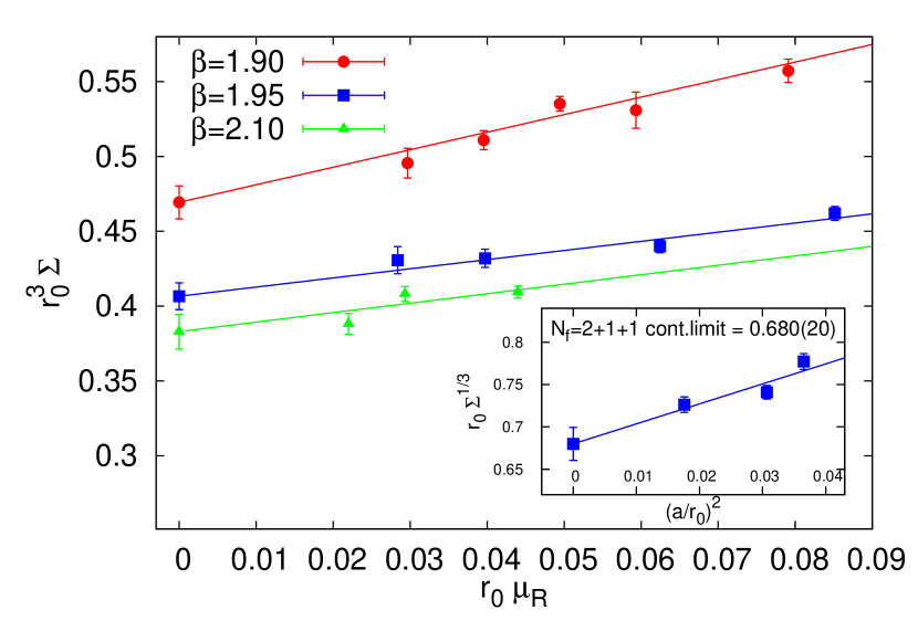
Figure 4: Main plot: chiral extrapolations of the chiral condensate $r_{0}^{3}\Sigma$ for $N_{f}=2+1+1$ ensembles and $\beta=1.9$, 1.95, 2.1. The lines are extrapolations to the chiral limit, linear in the quark mass. The errors are statistical only. Inset: continuum extrapolation of the chirally extrapolated chiral condensate $r_{0}\Sigma^{1/3}$ vs. $(a/r_{0})^{2}$. The errors include: statistical errors, errors from $Z_{P}$ and errors from $r_{0}/a$.

In Tab. 6, we show all our results for $r_{0}\Sigma^{1/3}$ in the 2+1+1-flavour case. We also include the results of a linear extrapolation to the chiral limit for each value of $\beta$, shown in the main plot of Fig. 4. As before, we plot only statistical errors, since all extrapolations are performed at fixed $\beta$ and the errors from $Z_{P}$ and $r_{0}/a$ are the same for all quark masses (we use chirally extrapolated values of $Z_{P}$ and $r_{0}/a$) – given in Tab. 6. Contrary to the $N_{f}=2$ case, the slope of the dependence of the mass-dependent condensate on the light quark mass slightly decreases for increasing $\beta$ (the change of slope is statistically significant when going from $\beta=1.9$ to $\beta=2.1$). This has the effect of lowering the systematic error related to the choice of the fitting range for decreasing lattice spacing, which is for all $\beta$ the dominating source of error (although for $\beta=2.1$ other errors become comparable).

The chirally extrapolated values at three lattice spacings are then used to perform an extrapolation to the continuum limit, which is again compatible with $\mathcal{O}(a^{2})$ cut-off effects. To estimate the fitting range uncertainty, we again perform 3 separate continuum limit extrapolations, using different fitting ranges and different values of $M_{R}$, corresponding to approx. 80, 90 and 100 MeV. The values of $r_{0}\Sigma^{1/3}$ in the continuum limit are, respectively, 0.668(24), 0.680(20) and 0.659(27). As our central value we take the result from the full fitting range:

$$r_{0}\Sigma^{1/3}_{N_{f}=2+1+1}=0.680(20)(21),$$

with the larger of the differences with respect to values from tailored fitting intervals as the fitting range systematic error. This can be compared to the 2-flavour result which amounts to $r_{0}\Sigma^{1/3}_{N_{f}=2}=0.689(16)(29)$ and both results are compatible within errors.

5 Conclusions

In this paper, we presented our results on the chiral condensate in QCD with $N_{f}=2$ and $N_{f}=2+1+1$ flavours of dynamical Wilson twisted mass quarks at maximal twist.

Our final results are:

$$r_{0}\Sigma^{1/3}_{N_{f}=2}=0.689(16)(29),$$

$$r_{0}\Sigma^{1/3}_{N_{f}=2+1+1}=0.680(20)(21),$$

which indicates that at the current level of precision, we cannot discriminate the influence of the dynamical strange and charm quarks on the value of the light quark chiral condensate.

The main source of the error of our results is the systematic error related to the choice of the fitting range in the dependence of the renormalized mode number on the renormalized spectral threshold. The second most important source of the error is either the statistical error or the error related to the uncertainty in the values of $r_{0}/a$ (which are inputs of our analysis). The error from $Z_{P}$ (also an input of our analysis), used to renormalize the quark masses and the spectral threshold parameter, is usually the smallest. However, we want to emphasize that in all cases the fitting range error is the largest one and in most cases it is larger by a factor of 2-4 than any other error. The rather small statistical errors that we obtain indicate that increasing statistics would not make our total error significantly smaller. This implies that a way to improve the total error would be to increase the number of values of the spectral threshold $M_{R}$ at which one computes the mode number. This would allow to identify more precisely the linear region of the mode number vs. $M_{R}$ dependence (see discussion in the Appendix) – on the one hand sufficiently far away from the renormalized quark mass, on the other hand low enough such that there are no deviations from the linear behaviour at the upper end of the fitting range (observed already at $M_{R}\approx 130$ MeV in the $N_{f}=2+1+1$ case).

Result	method	$N_{f}$	fermions	$r_{0}\Sigma^{1/3}$
this work	spectral proj.	2	twisted mass	0.689(16)(29)
this work	spectral proj.	2+1+1	twisted mass	0.680(20)(21)
RBC-UKQCD Aoki:2010dy	chiral fits	2+1	domain wall	0.632(15)(12)
MILC Bazavov:2009bb	chiral fits	2+1	staggered	0.654(14)(18)
MILC Bazavov:2010yq	chiral fits	2+1	staggered	0.653(18)(11)
S. Borsanyi et al. Borsanyi:2012zv	chiral fits	2+1	staggered	0.662(5)(20)
ETMC Baron:2009wt	chiral fits	2	twisted mass	0.575(14)(52)
ETMC Burger:2012ti	quark propagator	2	twisted mass	0.676(89)(14)
HPQCD McNeile:2012xh	quark propagator	2+1+1	staggered	0.673(5)(11)

Table 7: Comparison of our results for $r_{0}\Sigma^{1/3}$ with large-volume continuum limit results found in literature. In the given references, the values of $\Sigma$ are given in MeV. To convert to the dimensionless product $r_{0}\Sigma^{1/3}$, we combine them with results for $r_{0}$. The first error given is always from the computation of the value in MeV (when there are several errors given, we combine them in quadrature) and the second one from conversion using physical value of $r_{0}$. For RBC-UKQCD, $\Sigma^{1/3}=256(6)$ MeV, $r_{0}=0.487(9)$ fm Aoki:2010dy . For MILC Bazavov:2009bb , $\Sigma^{1/3}=278(6)$ MeV, $r_{1}=0.318(7)$ fm Bazavov:2009bb , $r_{0}/r_{1}$=1.46(1)(2) Bernard:2007ps . For MILC Bazavov:2010yq , $\Sigma^{1/3}=281.5(7.9)$ MeV, $r_{1}=0.3133(23)$ fm Bazavov:2010yq , $r_{0}/r_{1}$=1.46(1)(2) Bernard:2007ps . For S. Borsanyi et al. Borsanyi:2012zv , $\Sigma^{1/3}=272.3(1.2)(1.4)$ MeV, $r_{0}=0.48(1)(1)$ fm Aoki:2009sc . For ETMC Baron:2009wt , $\Sigma^{1/3}=269.9(6.5)$ MeV, $r_{0}=0.420(14)$ fm. However, newer analyses indicate a higher value of $r_{0}\approx 0.45$ fm Blossier:2010cr . To take this into account, we added the spread of the new and old value as a systematic error and used $r_{0}=0.420(38)$ fm to calculate $r_{0}\Sigma^{1/3}$ from $\Sigma^{1/3}$ in MeV. For ETMC Burger:2012ti , $\Sigma^{1/3}=299(26)(29)$ MeV, $r_{0}=0.446(9)$ fm Baron:2009wt . For HPQCD McNeile:2012xh , $\Sigma^{1/3}=283(2)$ MeV, $r_{1}=0.3209(26)$ fm Dowdall:2011wh , $r_{0}/r_{1}$=1.46(1)(2) Bernard:2007ps .

In order to place our values of the chiral condensate in context of results of other collaborations, we attempt in Tab. 7 a comparison. Given the large amount of approaches to compute the chiral condensate, as mentioned in the introduction, we make a selection by only considering results that are given in the literature as continuum limit values from large volume simulations. Note that the other available results that are listed in Tab. 7 are obtained in a different way than the spectral projector method. They mostly use chiral perturbation theory fits to the quark mass dependence of light pseudoscalar meson observables or determine the chiral condensate from the quark propagator. Not discussing the advantages or disadvantages of the various fermion discretizations used, we see in Tab. 7 an overall agreement for the dimensionless quantity $r_{0}\Sigma^{1/3}$, which is reassuring and establishes, in our opinion, the spectral projector method as a valuable alternative to determine the chiral condensate. On the other hand, when looking at the chiral condensate in physical units, see the caption of Tab. 7, a spread of results is obtained. Thus, it seems that the scale setting from the different lattice calculations introduces a systematic effect and it would be desirable to clarify this uncertainty in future more precise calculations.

Acknowledgments We thank the European Twisted Mass Collaboration for generating gauge field configurations ensembles used for this work. We are grateful to A. Shindler for discussions and in particular suggestions concerning $\mathcal{O}(a)$ improvement of the mode number. We thank G. Herdoiza for discussions at various stages of this work and for his careful reading of the manuscript. We acknowledge useful discussions with P. Damgaard, V. Drach, M. Lüscher, K. Ottnad, G.C. Rossi, S. Sharpe, C. Urbach, F. Zimmermann. K.C. was supported by Foundation for Polish Science fellowship “Kolumb”. This work was supported in part by the DFG Sonderforschungsbereich/Transregio SFB/TR9. K.J. was supported in part by the Cyprus Research Promotion Foundation under contract $\Pi$PO$\Sigma$E$\Lambda$KY$\Sigma$H/EM$\Pi$EIPO$\Sigma$/0311/16. The computer time for this project was made available to us by the Jülich Supercomputing Center, LRZ in Munich, the PC cluster in Zeuthen, Poznan Supercomputing and Networking Center (PCSS). We thank these computer centers and their staff for all technical advice and help.

Appendix A Testing the method

To test our implementation of the method in the tmLQCD package Jansen:2009xp , we compared the spectral projectors results for the mode number with ones from explicit computation of 150 lowest eigenvalues of $D^{\dagger}D$ for each gauge field configuration, using ensemble B85.24. The results of this comparison are shown in the right plot of Fig. 5, where the 4 points correspond to the stochastically evaluated mode number using spectral projectors, while the continuous line (which has an error roughly of the order of the width of the line) is the result from explicitly computing the eigenvalues. We observe very good agreement between the two methods.

Moreover, we used the results of explicit computation of eigenvalues to estimate the region of renormalized spectral threshold of $M_{R}$ where we observe linear dependence between the renormalized mode number and the threshold value (left plot of Fig. 5). The onset of non-linear behaviour corresponds to approx. 130-150 MeV. On the other end of the spectrum, one clearly observes effects of $M_{R}$ close to the renormalized quark mass up to around 10-20 MeV above the latter. This allows us to identify the linear region to extend between around 60 and 120 MeV, to allow for some safety margin. Therefore, we decided to choose our values of $M_{R}$ for the computation of the chiral condensate roughly in this interval. We remark that values in this range were used in Ref. Giusti:2008vb .

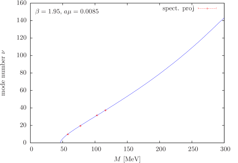
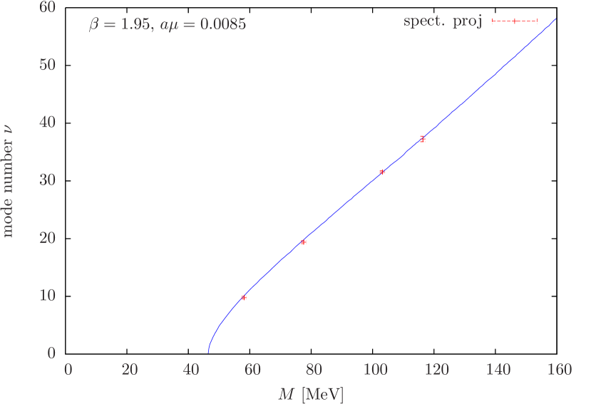
Figure 5: The mode number as a function of $M_{R}$ for the ensemble B85.24. The solid line in both plots is the result of explicit computation of 150 eigenvalues for each gauge field configuration, while data points represent results of spectral projectors calculation of the mode number for 4 values of $M_{R}$. The right plot is the zoom of the left part.

Some parameters employed in the method of spectral projectors need to be tuned to obtain a compromise between the accuracy of results and computational cost.

First of all, as mentioned in Ref. Giusti:2008vb , the precision of the inverter can be chosen to be relatively sloppy without reducing the accuracy. In order to identify the optimal precision, which does not affect the correctness of the result, but still decreases the computational time, we computed the mode number for several values of the relative precision of the inverter. The results (for ensemble b40.16) are shown in Fig. 6, which shows that even precision of $10^{-2}$ gives reasonable result. However, we decided to be conservative and we chose a value of $10^{-6}$ for the relative precision of the inverter.

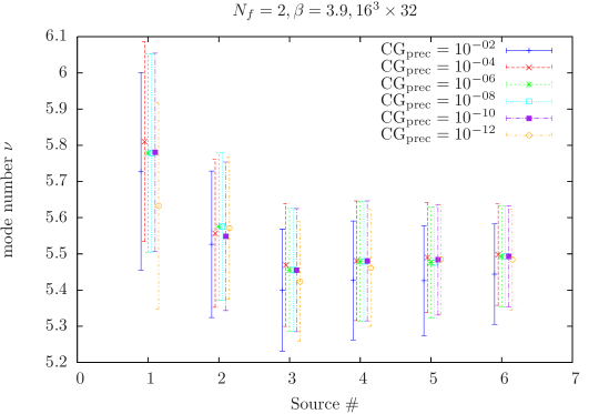
Figure 6: The mode number vs. the number of averaged stochastic sources using different values of the inverter relative precision for a $16^{3}\times 32$ lattice at $\beta=3.9$, $a\mu=0.004$ (ensemble b40.16).

We also checked the dependence of the mode number on the number of stochastic sources used for each gauge field configuration, shown again in Fig. 6. We observe that all results are compatible within error, which matches the suggestion of Ref. Giusti:2008vb that one stochastic source should be enough. However, we observe that adding a second source might help to considerably reduce the statistical error, which may be important for shorter Monte Carlo runs, when the available number of independent gauge field configurations is rather small. Adding further sources does not change the error considerably, because of correlations between results obtained from the same gauge field configuration.

Appendix B Autocorrelations

Ensemble	number	step	$\tau_{\rm int}$ (boot)	$\tau_{\rm int}$ (UW)	$\tau_{\rm int}$ (boot)	$\tau_{\rm int}$ (UW)
	of confs	HMC traj.	smallest $M$		largest $M$
A30.32	116	20	0.7	0.6(2)	1.7	1.9(8)
A40.20	197	16	0.8	0.9(3)	0.8	0.9(3)
A40.24	185	20	0.6	0.7(2)	1.5	2.2(8)
A40.32	201	8	0.8	0.7(2)	0.8	0.7(2)
A50.32	201	20	0.5	0.7(2)	0.5	0.8(2)
A60.24	161	8	0.7	0.5(1)	1.3	1.6(6)
A80.24	200	8	0.6	0.7(2)	0.7	0.9(2)
B25.32	200	20	1.0	0.7(2)	1.0	1.2(4)
B35.32	199	20	0.4	0.5(1)	1.0	1.7(6)
B55.32	201	20	0.4	0.4(1)	0.6	0.7(2)
B75.32	199	8	0.7	0.6(1)	0.5	0.5(1)
B85.24	196	20	0.4	0.4(1)	0.5	0.5(1)
D15.48	119	20	0.5	0.5(1)	0.6	0.8(2)
D20.48	193	20	0.6	0.5(1)	0.7	0.7(2)
D30.48	203	20	0.4	0.4(1)	0.5	0.4(1)

Table 8: Autocorrelations in the mode number, $N_{f}=2+1+1$ ensembles. We give the number of gauge field configurations used for each ensemble, the step in units of HMC trajectories and the calculated values of $\tau_{\rm int}$ using two methods: bootstrap with blocking (boot) and the method proposed by U. Wolff Wolff:2003sm (UW).

Ensemble	number	step	$\tau_{\rm int}$ (boot)	$\tau_{\rm int}$ (UW)	$\tau_{\rm int}$ (boot)	$\tau_{\rm int}$ (UW)
	of confs	HMC traj.	smallest $M$		largest $M$
b$30.32$	134	8	0.3	0.4(1)	0.9	0.9(3)
b$40.16$	544	10	0.5	0.5(1)	1.6	1.8(4)
b$40.20$	265	20	0.6	0.5(1)	1.2	1.3(3)
b$40.24$	465	20	0.5	0.7(2)	0.8	1.3(3)
b$40.32$	232	16	0.4	0.4(1)	0.5	0.5(1)
b$64.24$	272	20	0.4	0.4(1)	0.6	0.8(2)
b$85.24$	187	20	0.3	0.4(1)	0.5	0.5(1)
c$30.32$	183	8	0.7	0.5(1)	1.2	1.6(5)
c$60.32$	123	20	0.5	0.5(1)	0.4	0.5(1)
c$80.32$	201	10	0.4	0.5(1)	1.1	0.8(2)
d$20.48$	77	10	0.7	0.5(1)	0.5	0.6(2)
d$65.32$	199	20	0.6	0.5(1)	0.7	1.0(3)

Table 9: Autocorrelations in the mode number, $N_{f}=2$ ensembles. We give the number of gauge field configurations used for each ensemble, the step in units of HMC trajectories and the calculated values of $\tau_{\rm int}$ using two methods: bootstrap with blocking (boot) and the method proposed by U. Wolff Wolff:2003sm (UW).

In this appendix, we show the results of our autocorrelation analysis of the mode number (for the smallest and largest value of $M$ that we used for chiral condensate extraction). We applied two methods: bootstrap with blocking (with block size of 10 measurements) and the method proposed by U. Wolff in Ref. Wolff:2003sm . Our results are shown in Tabs. 8 ($N_{f}=2+1+1$) and 9 ($N_{f}=2$). In general, both methods yield compatible results for the integrated autocorrelation time $\tau_{\rm int}$ (in the case of the method of Ref. Wolff:2003sm , we quote also the error of $\tau_{\rm int}$ and the two values of $\tau_{\rm int}$ that we obtain agree within this error).

Our conclusions about the dependence of $\tau_{\rm int}$ on simulation parameters are the following:

• at the smallest value of $M$, no autocorrelations are observed ($\tau_{\rm int}$ compatible with 0.5),

• at the largest value of $M$, in some cases the autocorrelations become visible, with $\tau_{\rm int}$ between 1 and 2,

• there is a tendency towards larger autocorrelations for smaller quark masses (e.g. B25 compared to B85) and for smaller volumes (e.g. b40 ensembles at 4 volumes),

• we don’t observe a tendency towards increased $\tau_{\rm int}$ for decreasing lattice spacing.

References

- (1) PACS-CS Collaboration, S. Aoki et al., 2+1 Flavor Lattice QCD toward the Physical Point, Phys.Rev. D79 (2009) 034503, [arXiv:0807.1661].
- (2) RBC-UKQCD Collaboration, C. Allton et al., Physical Results from 2+1 Flavor Domain Wall QCD and SU(2) Chiral Perturbation Theory, Phys.Rev. D78 (2008) 114509, [arXiv:0804.0473].
- (3) RBC-UKQCD Collaboration, Y. Aoki et al., Continuum Limit Physics from 2+1 Flavor Domain Wall QCD, Phys.Rev. D83 (2011) 074508, [arXiv:1011.0892].
- (4) A. Bazavov, D. Toussaint, C. Bernard, J. Laiho, C. DeTar, et al., Nonperturbative QCD simulations with 2+1 flavors of improved staggered quarks, Rev.Mod.Phys. 82 (2010) 1349–1417, [arXiv:0903.3598].
- (5) A. Bazavov, C. Bernard, C. DeTar, X. Du, W. Freeman, et al., Staggered chiral perturbation theory in the two-flavor case and SU(2) analysis of the MILC data, PoS LATTICE2010 (2010) 083, [arXiv:1011.1792].
- (6) ETMC Collaboration, R. Baron et al., Light Meson Physics from Maximally Twisted Mass Lattice QCD, JHEP 1008 (2010) 097, [arXiv:0911.5061].
- (7) JLQCD, TWQCD Collaboration, H. Fukaya et al., Determination of the chiral condensate from QCD Dirac spectrum on the lattice, Phys.Rev. D83 (2011) 074501, [arXiv:1012.4052].
- (8) V. Bernard, S. Descotes-Genon, and G. Toucas, Topological susceptibility on the lattice and the three-flavour quark condensate, JHEP 1206 (2012) 051, [arXiv:1203.0508].
- (9) S. Borsanyi, S. Durr, Z. Fodor, S. Krieg, A. Schafer, et al., SU(2) chiral perturbation theory low-energy constants from 2+1 flavor staggered lattice simulations, arXiv:1205.0788.
- (10) S. Durr, Topological susceptibility in full QCD: Lattice results versus the prediction from the QCD partition function with granularity, Nucl.Phys. B611 (2001) 281–310, [hep-lat/0103011].
- (11) TWQCD Collaboration, T.-W. Chiu, T.-H. Hsieh, and P.-K. Tseng, Topological susceptibility in 2+1 flavors lattice QCD with domain-wall fermions, Phys.Lett. B671 (2009) 135–138, [arXiv:0810.3406].
- (12) T. W. Chiu, T. H. Hsieh, and Y. Y. Mao, Topological Susceptibility in Two Flavors Lattice QCD with the Optimal Domain-Wall Fermion, Phys.Lett. B702 (2011) 131–134, [arXiv:1105.4414].
- (13) F. Bernardoni, P. Hernandez, N. Garron, S. Necco, and C. Pena, Probing the chiral regime of = 2 QCD with mixed actions, Phys.Rev. D83 (2011) 054503, [arXiv:1008.1870].
- (14) ETMC Collaboration, R. Frezzotti, V. Lubicz, and S. Simula, Electromagnetic form factor of the pion from twisted-mass lattice QCD at N(f) = 2, Phys.Rev. D79 (2009) 074506, [arXiv:0812.4042].
- (15) P. Hernandez, K. Jansen, and L. Lellouch, Finite size scaling of the quark condensate in quenched lattice QCD, Phys.Lett. B469 (1999) 198–204, [hep-lat/9907022].
- (16) P. Damgaard, U. M. Heller, R. Niclasen, and K. Rummukainen, Eigenvalue distributions of the QCD Dirac operator, Phys.Lett. B495 (2000) 263–270, [hep-lat/0007041].
- (17) T. A. DeGrand and S. Schaefer, Chiral properties of two-flavor QCD in small volume and at large lattice spacing, Phys.Rev. D72 (2005) 054503, [hep-lat/0506021].
- (18) C. Lang, P. Majumdar, and W. Ortner, The Condensate for two dynamical chirally improved quarks in QCD, Phys.Lett. B649 (2007) 225–229, [hep-lat/0611010].
- (19) JLQCD Collaboration, H. Fukaya et al., Two-flavor lattice QCD simulation in the epsilon-regime with exact chiral symmetry, Phys.Rev.Lett. 98 (2007) 172001, [hep-lat/0702003].
- (20) TWQCD Collaboration, H. Fukaya et al., Two-flavor lattice QCD in the epsilon-regime and chiral Random Matrix Theory, Phys.Rev. D76 (2007) 054503, [arXiv:0705.3322].
- (21) A. Hasenfratz, R. Hoffmann, and S. Schaefer, Low energy chiral constants from epsilon-regime simulations with improved Wilson fermions, Phys.Rev. D78 (2008) 054511, [arXiv:0806.4586].
- (22) K. Jansen and A. Shindler, The Epsilon regime of chiral perturbation theory with Wilson-type fermions, PoS LAT2009 (2009) 070, [arXiv:0911.1931].
- (23) K. Splittorff and J. Verbaarschot, The Microscopic Twisted Mass Dirac Spectrum, Phys.Rev. D85 (2012) 105008, [arXiv:1201.1361].
- (24) S. Necco and A. Shindler, Spectral density of the Hermitean Wilson Dirac operator: a NLO computation in chiral perturbation theory, JHEP 1104 (2011) 031, [arXiv:1101.1778].
- (25) S. Necco and A. Shindler, On the spectral density of the Wilson operator, PoS LATTICE2011 (2011) 250, [arXiv:1108.1950].
- (26) S. Necco and A. Shindler, Corrections to the Banks-Casher relation with Wilson quarks, arXiv:1302.5595.
- (27) F. Burger, V. Lubicz, M. Muller-Preussker, S. Simula, and C. Urbach, Quark mass and chiral condensate from the Wilson twisted mass lattice quark propagator, arXiv:1210.0838.
- (28) C. McNeile, A. Bazavov, C. Davies, R. Dowdall, K. Hornbostel, et al., Direct determination of the strange and light quark condensates from full lattice QCD, arXiv:1211.6577.
- (29) G. Colangelo, S. Durr, A. Juttner, L. Lellouch, H. Leutwyler, et al., Review of lattice results concerning low energy particle physics, Eur.Phys.J. C71 (2011) 1695, [arXiv:1011.4408].
- (30) T. Banks and A. Casher, Chiral Symmetry Breaking in Confining Theories, Nucl.Phys. B169 (1980) 103.
- (31) L. Giusti and M. Luscher, Chiral symmetry breaking and the Banks-Casher relation in lattice QCD with Wilson quarks, JHEP 0903 (2009) 013, [arXiv:0812.3638].
- (32) K. Cichy, V. Drach, E. Garcia-Ramos, and K. Jansen, Topological susceptibility and chiral condensate with dynamical flavors of maximally twisted mass fermions, PoS LATTICE2011 (2011) 102, [arXiv:1111.3322].
- (33) ETMC Collaboration, P. Boucaud et al., Dynamical twisted mass fermions with light quarks, Phys.Lett. B650 (2007) 304–311, [hep-lat/0701012].
- (34) ETMC Collaboration, P. Boucaud et al., Dynamical Twisted Mass Fermions with Light Quarks: Simulation and Analysis Details, Comput.Phys.Commun. 179 (2008) 695–715, [arXiv:0803.0224].
- (35) ETMC Collaboration, R. Baron, P. Boucaud, J. Carbonell, A. Deuzeman, V. Drach, et al., Light hadrons from lattice QCD with light (u,d), strange and charm dynamical quarks, JHEP 1006 (2010) 111, [arXiv:1004.5284].
- (36) ETMC Collaboration, R. Baron et al., Computing K and D meson masses with = 2+1+1 twisted mass lattice QCD, Comput.Phys.Commun. 182 (2011) 299–316, [arXiv:1005.2042].
- (37) ETMC Collaboration, R. Baron et al., Light hadrons from Nf=2+1+1 dynamical twisted mass fermions, PoS LATTICE2010 (2010) 123, [arXiv:1101.0518].
- (38) P. Weisz, Continuum Limit Improved Lattice Action for Pure Yang-Mills Theory. 1., Nucl.Phys. B212 (1983) 1.
- (39) Y. Iwasaki, Renormalization Group Analysis of Lattice Theories and Improved Lattice Action: Two-Dimensional Nonlinear O(N) Sigma Model, Nucl.Phys. B258 (1985) 141–156.
- (40) Y. Iwasaki, K. Kanaya, T. Kaneko, and T. Yoshie, Scaling in SU(3) pure gauge theory with a renormalization group improved action, Phys.Rev. D56 (1997) 151–160, [hep-lat/9610023].
- (41) Alpha Collaboration, R. Frezzotti, P. A. Grassi, S. Sint, and P. Weisz, Lattice QCD with a chirally twisted mass term, JHEP 0108 (2001) 058, [hep-lat/0101001].
- (42) R. Frezzotti and G. Rossi, Chirally improving Wilson fermions. 1. O(a) improvement, JHEP 0408 (2004) 007, [hep-lat/0306014].
- (43) R. Frezzotti and G. Rossi, Chirally improving Wilson fermions. II. Four-quark operators, JHEP 0410 (2004) 070, [hep-lat/0407002].
- (44) A. Shindler, Twisted mass lattice QCD, Phys.Rept. 461 (2008) 37–110, [arXiv:0707.4093].
- (45) R. Frezzotti and G. Rossi, Twisted mass lattice QCD with mass nondegenerate quarks, Nucl.Phys.Proc.Suppl. 128 (2004) 193–202, [hep-lat/0311008].
- (46) T. Chiarappa, F. Farchioni, K. Jansen, I. Montvay, E. Scholz, et al., Numerical simulation of QCD with u, d, s and c quarks in the twisted-mass Wilson formulation, Eur.Phys.J. C50 (2007) 373–383, [hep-lat/0606011].
- (47) F. Farchioni, C. Urbach, R. Frezzotti, K. Jansen, I. Montvay, et al., Exploring the phase structure of lattice QCD with twisted mass quarks, Nucl.Phys.Proc.Suppl. 140 (2005) 240–245, [hep-lat/0409098].
- (48) F. Farchioni, K. Jansen, I. Montvay, E. Scholz, L. Scorzato, et al., The Phase structure of lattice QCD with Wilson quarks and renormalization group improved gluons, Eur.Phys.J. C42 (2005) 73–87, [hep-lat/0410031].
- (49) R. Frezzotti, G. Martinelli, M. Papinutto, and G. Rossi, Reducing cutoff effects in maximally twisted lattice QCD close to the chiral limit, JHEP 0604 (2006) 038, [hep-lat/0503034].
- (50) XLF Collaboration, K. Jansen, M. Papinutto, A. Shindler, C. Urbach, and I. Wetzorke, Quenched scaling of Wilson twisted mass fermions, JHEP 0509 (2005) 071, [hep-lat/0507010].
- (51) ETMC Collaboration, B. Blossier et al., Average up/down, strange and charm quark masses with Nf=2 twisted mass lattice QCD, Phys.Rev. D82 (2010) 114513, [arXiv:1010.3659].
- (52) ETMC Collaboration, K. Ottnad et al., and mesons from Nf=2+1+1 twisted mass lattice QCD, JHEP 1211 (2012) 048, [arXiv:1206.6719].
- (53) ETMC Collaboration, M. Constantinou et al., Non-perturbative renormalization of quark bilinear operators with Nf = 2 (tmQCD) Wilson fermions and the tree-level improved gauge action, JHEP 1008 (2010) 068, [arXiv:1004.1115].
- (54) C. Alexandrou, M. Constantinou, T. Korzec, H. Panagopoulos, and F. Stylianou, Renormalization constants of local operators for Wilson type improved fermions, Phys.Rev. D86 (2012) 014505, [arXiv:1201.5025].
- (55) ETMC preliminary result for renormalization constants, private communication from D. Palao.
- (56) ETMC Collaboration, P. Dimopoulos et al., Renormalization constants for Wilson fermion lattice QCD with four dynamical flavours, PoS LATTICE2010 (2010) 235, [arXiv:1101.1877].
- (57) ETMC Collaboration, B. Blossier et al., Renormalisation constants of quark bilinears in lattice QCD with four dynamical Wilson quarks, PoS LATTICE2011 (2011) 233, [arXiv:1112.1540].
- (58) ETMC Collaboration, C. Alexandrou et al., Light baryon masses with dynamical twisted mass fermions, Phys.Rev. D78 (2008) 014509, [arXiv:0803.3190].
- (59) K. Cichy, E. Garcia-Ramos, K. Jansen, and A. Shindler in preparation.
- (60) C. Bernard, C. E. DeTar, L. Levkova, S. Gottlieb, U. Heller, et al., Status of the MILC light pseudoscalar meson project, PoS LAT2007 (2007) 090, [arXiv:0710.1118].
- (61) Y. Aoki, S. Borsanyi, S. Durr, Z. Fodor, S. D. Katz, et al., The QCD transition temperature: results with physical masses in the continuum limit II., JHEP 0906 (2009) 088, [arXiv:0903.4155].
- (62) HPQCD Collaboration, R. Dowdall et al., The Upsilon spectrum and the determination of the lattice spacing from lattice QCD including charm quarks in the sea, Phys.Rev. D85 (2012) 054509, [arXiv:1110.6887].
- (63) K. Jansen and C. Urbach, tmLQCD: A Program suite to simulate Wilson Twisted mass Lattice QCD, Comput.Phys.Commun. 180 (2009) 2717–2738, [arXiv:0905.3331].
- (64) ALPHA Collaboration, U. Wolff, Monte Carlo errors with less errors, Comput.Phys.Commun. 156 (2004) 143–153, [hep-lat/0306017].