The large-scale Quasar-Lyman $\alpha$ Forest Cross-Correlation from BOSS

Abstract

We measure the large-scale cross-correlation of quasars with the Ly$\alpha$ forest absorption in redshift space, using $\sim 60000$ quasar spectra from Data Release 9 (DR9) of the Baryon Oscillation Spectroscopic Survey (BOSS). The cross-correlation is detected over a wide range of scales, up to comoving separations $r$ of $80$ $\,h^{-1}\,{\rm Mpc}$. For $r>15\,h^{-1}\,{\rm Mpc}$, we show that the cross-correlation is well fitted by the linear theory prediction for the mean overdensity around a quasar host halo in the standard $\,\rm\Lambda$CDM model, with the redshift distortions indicative of gravitational evolution detected at high confidence. Using previous determinations of the Ly$\alpha$ forest bias factor obtained from the Ly$\alpha$ autocorrelation, we infer the quasar bias factor to be $b_{q}=3.64^{+0.13}_{-0.15}$ at a mean redshift $z=2.38$, in agreement with previous measurements from the quasar auto-correlation. We also obtain a new estimate of the Ly$\alpha$ forest redshift distortion factor, $\beta_{F}=1.1\pm 0.15$, slightly larger than but consistent with the previous measurement from the Ly$\alpha$ forest autocorrelation. The simple linear model we use fails at separations $r<15\,h^{-1}\,{\rm Mpc}$, and we show that this may reasonably be due to the enhanced ionization due to radiation from the quasars. We also provide the expected correction that the mass overdensity around the quasar implies for measurements of the ionizing radiation background from the line-of-sight proximity effect.

1 Introduction

As the most optically luminous objects known in the universe, quasars are used as lampposts at high redshift to obtain absorption spectra of the intervening intergalactic medium, as well as tracers of large-scale structure. Their absorption spectra blueward of the Ly$\alpha$ emission line reveal the Ly$\alpha$ forest, reflecting the structure in the hydrogen gas density in the intergalactic medium as it evolves through gravitational collapse around dark matter halos in which galaxies form (e.g., [1],[2], [3], [4]).

The large-scale clustering of quasars was measured in the 2dF survey (e.g. [5], [6], [7]) and in the Sloan Digital Sky Survey (SDSS, [8], [9], [10]). Both the Ly$\alpha$ forest and the quasar clustering can be used as tracers of the underlying large-scale mass fluctuations, which are thought to have an origin in the initial conditions of the universe. In the linear regime, the observed quasar correlation function should be equal to the mass autocorrelation times the square of the mean bias factor of the quasar host halos. Recent results from the analyses of data from large-scale surveys have indicated a bias factor that increases with redshift and has a value $b_{q}=3.8\pm 0.3$ at $z=2.4$, and is nearly independent of quasar luminosity (see [11], [12]).

Quasar clustering can also be probed by means of the cross-correlation with other tracers. The quasar cross-correlation with galaxies was measured by [13], [14] and [15]. These studies found that the quasar bias factor has a value near unity, comparable to typical star-forming galaxies, at redshift $z\lesssim 1$, but the small samples at higher redshift already indicated a larger clustering amplitude. Quasars can also be cross-correlated with absorption systems found in the spectra of other quasars. This can be done with the hydrogen Ly$\alpha$ forest, with a high abundance of absorption features, and also with more sparse metal line systems such as the CIV lines, which was recently accomplished by [16].

The cross-correlation of quasars with the Ly$\alpha$ forest absorption was first searched for along the same line of sight of each individual quasar, looking for the impact of the quasar ionizing radiation reducing the Ly$\alpha$ absorption, which has been designated as “proximity effect” or “inverse effect” ([17], [18], [19]). The ionizing radiation emitted by a quasar is added to the intensity of the cosmic ionizing background, and the higher than average intensity in the quasar vicinity implies an increased degree of ionization of the intergalactic medium, and therefore a decreased absorption by the Ly$\alpha$ forest. Studies of the proximity effect have therefore expected a lower than average absorption of the Ly$\alpha$ forest near the quasar Ly$\alpha$ emission line compared to the absorption at the same redshift seen in quasars at higher redshift, using this to infer the intensity of the cosmic ionizing background (see [20] for a more recent study). These investigations have generally not included in the analysis the fact that the intergalactic gas should have higher density near a quasar, because of the positive correlation of the quasar host halo with the mass density. In reality, the observations of the quasar-Ly$\alpha$ absorption cross-correlation should reveal the combined effect of the mean overdensity and the additional ionizing intensity around quasars, which substantially complicates the theoretical interpretation.

In general, the quasar-Ly$\alpha$ cross-correlation can be measured in redshift space from Ly$\alpha$ forest lines of sight near another quasar, as a function of the perpendicular and parallel components of the separation, $\sigma$ and $\pi$, respectively. The effect of a quasar on the Ly$\alpha$ forest in the spectrum of another nearby quasar was investigated in several papers that examined individual quasar pairs, generally separated by a few arc minutes ([21], [22], [23], [24]). These observations generally found no evidence for any decrease of Ly$\alpha$ absorption near quasars due to the excess ionizing radiation. In fact, both in the case of quasar pairs at small separation, and in the case of using a larger number of pairs at wider separations, it has been found that the Ly$\alpha$ absorption is stronger near quasars, rather than weaker ([25], [26], [27], [28],[29]), [30]. This result has been attributed to the mean overdensity near a quasar, combined with the reduction of the ionizing intensity from the quasar due to both anisotropic emission and time variability of the quasars, as discussed by [23], [26] and [27]. These works obtained upper limits to the luminosity of the quasars emitted in the perpendicular direction with a time delay, although no detailed analysis was done to attempt to model the effect of the overdensity and provide a robust interpretation of the data.

This question can now be investigated with the large sample of quasar spectra provided by the Baryon Oscillation Spectroscopic Survey (BOSS) of the SDSS-III Collaboration ([31], [32]). The DR9 Catalogue of quasars ([33]) already contains 87822 quasars, with more than 60000 of them at $z>2$, distributed over 3275 square degrees of the sky. The extensive area covered and the large number of quasars makes this sample particularly useful to study the quasar-Ly$\alpha$ cross-correlation at large scales (i.e., the typical nearest neighbor projected separation of $\sim 10\,h^{-1}\,{\rm Mpc}$ and larger).

At these separations, the cross-correlation function induced by the mass overdensity around quasars can be predicted from linear theory, and should be proportional to the product of the bias factors of the quasars and the Ly$\alpha$ forest and show the expected redshift distortions ([34], [35]). These bias factors can be independently determined by observations of the autocorrelations of the Ly$\alpha$ forest and the quasars ([4], [12]), and should agree with the measured amplitude of the cross-correlation.

This paper presents the quasar-Ly$\alpha$ cross correlation measured from the quasars in the DR9 catalogue of BOSS. The data sample is presented in section 2, and the method of analysis in section 3. Linear theory is used to model the mean cross-correlation, and the fits to the observational results are presented in section 4, showing that the overdensity effect alone adequately matches the results at comoving separations $r>15\,h^{-1}\,{\rm Mpc}$ for reasonable values of the bias factors. Section 5 discusses the expected effect of the ionizing radiation of the quasars on the cross-correlation for the quasar luminosities in our sample, and the manner that this may impact the results in section 4. Our conclusions are summarized in section 6.

Throughout this paper we use the flat $\,\rm\Lambda$CDM cosmology, with $\Omega_{m}=0.281$, $\Omega_{b}=0.0462$, $h=0.71$, $n_{s}=0.963$ and $\sigma_{8}=0.8$, consistent with the cosmological parameters from the WMAP mission [36].

2 Data Set

The data used in this paper is from the publicly available 9th Data Release (DR9, [37]) of the SDSS-III Collaboration ([31], [38], [39], [40], [41], [42], [43]), comprising the first two years of observations of the Baryon Oscillation Spectroscopic Survey (BOSS, [32]). The quasar sample is a subsample of the catalogue described in [33], while the Ly$\alpha$ absorption sightlines make use of the products described in [44].

We first describe the cuts we apply to the catalogue to select our quasar sample, and then the set of quasar lines of sight that we use for the Ly$\alpha$ absorption field to be cross-correlated with the quasars.

2.1 Quasar sample

A total of 87822 quasars are present in the DR9 quasar catalogue ([33]). These quasars were targeted for spectroscopy using a complex target selection procedure presented in [45] that combines a series of methods described in [46], [47], and [48]. The French Participation Group (FPG) of the SDSS-III Collaboration verified each of these objects by visually inspecting the spectra. A number of estimates of the quasar redshift based on different methods are provided in this catalogue. We generally use the redshift obtained using the Principal Component Analysis method (Z_PCA in DR9Q), but in Section 4.6 we examine our results for the quasar-Ly$\alpha$ cross-correlation when using other estimates for the quasar redshifts.

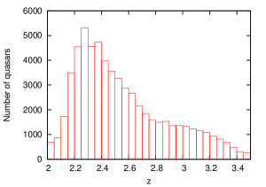
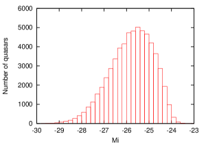
In order to have a well defined redshift interval in our sample, we use only the 61366 quasars with a redshift in the range $2<z_{q}<3.5$. Most of the 26456 quasars discarded by this criteria are at a redshift that is too low to be cross-correlated with the observed Ly$\alpha$ absorption spectra, and the few at $z_{q}>3.5$ have too few high-redshift nearby lines of sight to yield useful results. Finally, we apply a cut in $i$-band absolute magnitude, $-30<M_{i}<-23$, which reduces the final sample to 61342 quasars. The magnitudes are provided in the quasar catalog ([33]), and were computed using a similar cosmological model than the one used in this study. The redshift and $i$-band absolute magnitude distributions of our quasar sample are shown in figure 1.

Figure 1: Left panel: Distribution of the 61342 quasar redshifts in our sample. Right panel: $i$-band absolute magnitude distribution.

2.2 Ly$\alpha$ sample

Not all quasars present in the catalogue are useful and free of systematic effects for using the Ly$\alpha$ forest spectrum: they may be affected by broad absorption lines, they may have too low a redshift so that their Ly$\alpha$ forest pixels lie in the noisy blue end of the BOSS spectrograph, or their continuum may be too difficult to model. For these reasons, we select the same quasars as in [49], a previous study of the cross-correlation of the Ly$\alpha$ forest with Damped Ly$\alpha$ Systems (DLAs) using the DLA catalogue of [50]. This reduces the number of available lines of sight to $52449$. The selection criteria are that the quasar redshift lies in the range $2.15<z<3.5$, that the BAL_FLAG_VI flag is not set in the catalogue of [33], and that the median signal-to-noise ratio per pixel (of width $\sim 69\,{\rm km\,s}^{-1}$) in the quasar rest-frame wavelength range $1220{\,\rm\AA}\leq\lambda_{r}\leq 1600{\,\rm\AA}$ is $S/N>0.5$.

We define the Ly$\alpha$ forest region as the rest-frame wavelength range $1041{\,\rm\AA}\leq\lambda_{r}\leq 1185{\,\rm\AA}$, and use the ‘value-added’ co-added spectra made publicly available with DR9 ([44]), removing any pixels with the bit mask or the sky mask set, as defined in [44]. We also correct the pipeline estimate of the noise variance using the recipe described in [44].

Lines of sight that include no more than one detected DLA from the “DLA concordance catalogue” in [51] are included in the analysis, after masking the central region of the DLA absorption line and correcting for the damped wings outside this central region, as explained in [44]. Since the catalogue of [51] is not complete (especially in low S/N spectra), some residual contamination of DLAs is expected.

3 Method

The method we use to measure the quasar-Ly$\alpha$ cross-correlation is the same one as for the cross-correlation of Damped Lyman Alpha systems (DLAs) with the Ly$\alpha$ absorption, described in [49]. Here, a brief summary of the method is presented, discussing in detail only the issues that are special for our analysis of the quasar cross-correlation and any differences with respect to the method used for DLAs.

The observed flux in each pixel of the quasar spectra is $f_{i}=C_{i}\,\bar{F}(z_{i})\left[1+\delta_{Fi}\right]+N_{i}$, where $C_{i}$ is the quasar continuum (equal to the flux that would be observed in the absence of absorption), $\bar{F}(z_{i})$ is the mean transmitted fraction, $\delta_{Fi}$ is the Ly$\alpha$ transmission fluctuation, and $N_{i}$ is the observational noise, which is assumed to be uncorrelated in all pixel pairs. To estimate $\delta_{Fi}$ and its cross-correlation we must first model the continua of the quasars. This is done using the PCA technique described in [52], but without applying the Mean Flux Regulation described in this paper, which can suppress the large-scale power in the Ly$\alpha$ forest in ways that are difficult to model. In the same way as in [49], we generally apply instead the Mean Transmission Correction (hereafter MTC), which enforces the mean transmission in each quasar spectrum to be equal to the value measured in independent observations by [53], using equations (3.5) and (3.6) in [49]. This correction is useful to remove the broadband noise caused by spectrophotometric errors, but we will also show results when no correction to the quasar continua is applied. We will see in section 4 that including the MTC increases the accuracy of the measured quasar bias in our parameterized model by $\sim 30\%$. However, this correction distorts the cross-correlation function and the fitted theoretical model must be corrected to take this effect into account (see Appendix A in [49]).

The mean transmitted fraction $\bar{F}_{i}$ is measured here in 150 bins of $\Delta z=0.01$ over the range $1.9<z<3.4$ (no Ly$\alpha$ forest data is used outside this range). These redshift bins are three times smaller than the ones used in [49] for the same purpose. The measured $\bar{F}(z_{i})$ has fluctuations when using small redshift bins owing to systematic errors in the calibrating reference stars ([54], [44]), and we found that the fine redshift bins are necessary to correctly eliminate the effect of these fluctuations. In general, the larger number of available quasars compared to DLAs allows for a more accurate measurement of the cross-correlation for the quasars, and therefore greater care needs to be taken in the analysis for quasars.

The cross-correlation is computed with the simple estimator (see Appendix B of [49] for a discussion of the approximations involved and the differences with an optimal estimator):

$$\hat{\xi}_{A}=\frac{\sum_{i\in A}w_{i}\,\delta_{Fi}}{\sum_{i\in A}w_{i}}~{},$$ (3.1)

where the summation is done over all quasars and over all Ly$\alpha$ pixels that are within a bin ($A$) of the separation from each quasar in the perpendicular ($\sigma$) and parallel ($\pi$) directions, $\delta_{Fi}$ is the estimated value of the transmission fluctuation from the observed flux and the continuum model, and the weights $w_{i}$ are computed independently at each pixel from the noise $N_{i}$ provided for the DR9 data [38], assuming a model for the intrinsic Ly$\alpha$ absorption variance that is added in quadrature to the noise (equation 3.10 in [49]).

A set of 9 bins in $\sigma$ and 18 bins in $\pi$ are used to measure the cross-correlation, which are the same ones as in [49] except that we add the extra bin at large separations $60\,h^{-1}\,{\rm Mpc}<\sigma<80\,h^{-1}\,{\rm Mpc}$, and the same for both signs of $\pi$ (the cross-correlation is measured without assuming symmetry with respect to a sign change of the parallel separation $\pi$). This procedure yields a total of 162 bins. The weighted average values of $(\pi,\sigma$) of all the contributing pixel pairs to every bin $A$ are computed together with the cross-correlation from equation (3.1), using the same weights. These averages are generally close but not exactly equal to the central values of each bin. The models to be fitted are evaluated at these weighted averages of $(\sigma,\pi)$. A single redshift bin is generally used for the mean redshift $z$ of the Ly$\alpha$ forest pixel and the quasar, which is required to be in the range $2.0<z<3.5$, although some results are also presented in the next section using three redshift bins for the purpose of testing redshift evolution.

The errors of the cross-correlation are computed in two different ways: 1) The covariance matrix is estimated assuming Gaussianity and a model power spectrum for the Ly$\alpha$ forest intrinsic autocorrelation. 2) Our quasar sample is divided into twelve subsamples in adjacent areas of the sky, and the cross-correlation is computed separately in each subsample to infer bootstrap errors. The method used and the subsample areas are the same as in [49]. The covariance matrix is computed including only pixel pairs up to a transverse separation $\sigma<5\,h^{-1}\,{\rm Mpc}$ in order to make the computer time required for the calculation more manageable. Most of the contributions to the covariance comes from pixel pairs in the same line of sight ($\sigma=0$).

We use the same linear theory model described in Section 3.6 of [49] (their equation 3.16), with bias parameters $b_{q}$ and $b_{F}$, and redshift distortion parameters $\beta_{q}$ and $\beta_{F}$, for the quasars and the Ly$\alpha$ forest, respectively. The quasar redshift distortion parameter obeys the relation $\beta_{q}=f(\Omega)/b_{q}$, and for the Ly$\alpha$ forest we impose the condition $b_{F}(1+\beta_{F})=-0.336$ from the observational result of [4] obtained from the measured Ly$\alpha$ autocorrelation at $z=2.25$. We also impose that $\beta_{F}$ and $b_{q}$ are constant with redshift and $b_{F}\propto(1+z)^{2.9}$, as discussed in [4]. However, whereas the effect of redshift errors for DLAs could be neglected, this is not the case for quasars. We therefore add two extra free parameters to the model: a dispersion $\epsilon_{z}$ and a mean offset $\Delta_{z}$ of the quasar redshift error, assuming these errors to be Gaussian. The theoretical model for the linear cross-correlation is smoothed with a Gaussian in the parallel direction with this dispersion and offset.

Fits to this model are generally done using only separation bins at $r=(\sigma^{2}+\pi^{2})^{1/2}>15\,h^{-1}\,{\rm Mpc}$ in order to avoid the near region that is possibly affected by radiation and non-linear effects, although some fits will also be shown using all bins at $r>7\,h^{-1}\,{\rm Mpc}$. The theoretical prediction is corrected for the MTC using the equations explained in Appendix A of [49].

4 Results

4.1 Fiducial model

Figure 2: Measured cross-correlation in the indicated bins of perpendicular separation $\sigma$, as a function of the parallel separation $\pi$. The data points in green have a total separation $r=(\sigma^{2}+\pi^{2})^{1/2}<15\,h^{-1}\,{\rm Mpc}$, and are not used in most of our fits. Solid (dashed) dark (blue) lines show the best fit model for the fiducial analysis, when using bins with separations down to $r=15\,h^{-1}\,{\rm Mpc}$ ($r=7\,h^{-1}\,{\rm Mpc}$).

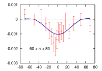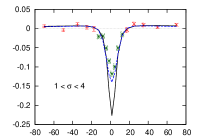
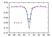
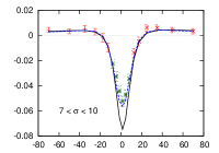
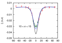
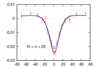
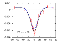
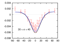
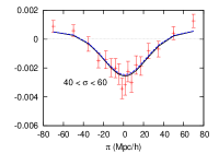
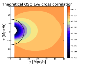
The results of the cross-correlation of the Ly$\alpha$ transmission with quasars, with the method presented in section 3, are shown in figure 2 for each bin in the transverse separation $\sigma$. The error bars are the diagonal elements of the computed covariance matrix, which we have found to be consistent with the bootstrap errors from the scatter of the cross-correlation function measured in subsamples. Two model fits to the data are also plotted in figure 2: the solid (black) line uses only bins with separation $r=(\sigma^{2}+\pi^{2})^{1/2}>15\,h^{-1}\,{\rm Mpc}$, and the dashed (blue) line uses all the bins with $r>7\,h^{-1}\,{\rm Mpc}$. The data points in green have a separation $r<15\,h^{-1}\,{\rm Mpc}$ and are not used in our main analysis. The same results are shown as contour plots in the left panel of figure 3, with our best fit fiducial model, the one using only the $r>15\,h^{-1}\,{\rm Mpc}$ bins, shown in the right panel.

Figure 3: Two dimensional contours of the measured cross-correlation (left panel), compared to the best fit theoretical models for $r>15\,h^{-1}\,{\rm Mpc}$ (right panel). The black circle corresponds to $r=15\,h^{-1}\,{\rm Mpc}$.

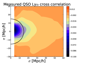
Our fiducial model fit applies the MTC to the data and includes the corresponding correction to the theory, and uses the whole sample of 61342 quasars described in section 2 with the PCA quasar redshifts. The model has four free parameters, as described at the end of section 3: $\beta_{F}$ (the Ly$\alpha$ redshift space distortion parameter), $b_{q}$ (the quasar bias factor), $\epsilon_{z}$ (the rms of the quasar redshift error distribution), and $\Delta_{z}$ (the mean offset of the quasar redshift), while the Ly$\alpha$ forest bias parameter $b_{F}$ is computed for each value of $\beta_{F}$ using the well-constrained quantity $b_{F}(1+\beta_{F})=-0.336$ at $z=2.25$ from the Ly$\alpha$ autocorrelation result of [4]. The first row in table 1 gives the parameters for the best fit result (in the sense of minimum value of $\chi^{2}$) using the covariance matrix as described earlier, with the value of $\chi^{2}$ and the number of degrees of freedom given in the last column. Errors correspond to the contours of $\Delta\chi^{2}=1$, after marginalizing over all other parameters. In the case of $\epsilon_{z}$, only an upper limit is provided when $\epsilon_{z}=0$ is within the $\Delta\chi^{2}=1$ contour. The parameters for other models that will be described below are given in the additional rows of the table. The variables related to quasar redshift errors, $\epsilon_{z}$ and $\Delta_{z}$, are expressed in units of $\,{\rm km\,s}^{-1}$, reflecting the directly-measured separation along the line of sight.

	$\beta_{F}$	$b_{q}$	$\epsilon_{z}(\,{\rm km\,s}^{-1})$	$\Delta_{z}(\,{\rm km\,s}^{-1})$	$\chi^{2}$ (d.o.f)
FIDUCIAL	$1.1^{+0.17}_{-0.15}$	$3.64^{+0.13}_{-0.15}$	$<370$	$-157^{+38}_{-36}$	116 (130)
$r>7\,h^{-1}\,{\rm Mpc}$	$1.67^{+0.23}_{-0.18}$	$3.34^{+0.12}_{-0.16}$	$433^{+44}_{-60}$	$-136^{+20}_{-19}$	164 (152)
NOCOR	$3.38^{+0.68}_{-0.77}$	$4^{+0.15}_{-0.18}$	$591^{64}_{-120}$	$-147^{+33}_{-32}$	142 (130)
NOMTC	$0.67^{+0.18}_{-0.11}$	$3.58^{+0.18}_{-0.15}$	$<280$	$-152^{+34}_{-37}$	112 (130)
LOW-Z	$1.81^{+0.56}_{-0.44}$	$3.79^{+0.31}_{-0.33}$	$660^{+137}_{-167}$	$-134^{+70}_{-54}$	124 (130)
MID-Z	$1.14^{+0.26}_{-0.26}$	$3.34^{+0.21}_{-0.24}$	$<450$	$-115^{+63}_{-50}$	131 (130)
HIGH-Z	$1.19^{+0.35}_{-0.25}$	$3.88^{+0.29}_{-0.3}$	$<428$	$-226^{+70}_{-62}$	134 (130)
LOW-L	$1.09^{+0.29}_{-0.18}$	$3.65^{+0.25}_{-0.2}$	$<340$	$-151^{+58}_{-56}$	128 (130)
MID-L	$1.03^{+0.36}_{-0.32}$	$3.29^{+0.27}_{-0.24}$	$<630$	$-113^{+56}_{-61}$	113 (130)
HIGH-L	$1.41^{+0.51}_{-0.24}$	$4.21^{+0.26}_{-0.26}$	$394^{+170}_{-220}$	$-189^{+46}_{-69}$	118 (130)
Z_VISUAL	$1.2^{+0.23}_{-0.16}$	$3.65^{+0.14}_{-0.16}$	$399^{+110}_{-99}$	$-231^{+28}_{-38}$	142 (130)
Z_PIPELINE	$1.13^{+0.21}_{-0.21}$	$3.4^{+0.15}_{-0.16}$	$546^{+86}_{-100}$	$-154^{+43}_{-24}$	114 (130)
Z_CIV	$1.34^{+0.19}_{-0.17}$	$3.66^{+0.13}_{-0.15}$	$503^{+72}_{-79}$	$-412^{+28}_{-36}$	137 (130)
Z_CIII	$1.44^{+0.26}_{-0.21}$	$3.5^{+0.2}_{-0.17}$	$648^{+87}_{-67}$	$-436^{+48}_{-34}$	137 (130)
Z_MgII	$1.73^{+0.44}_{-0.39}$	$3.55^{+0.26}_{-0.19}$	$636^{+110}_{-150}$	$-79^{+38}_{-56}$	126 (130)

Table 1: Best fit parameters and $\chi^{2}$ for the different analyses: FIDUCIAL (with the MTC and the corrected theory, using $r>15\,h^{-1}\,{\rm Mpc}$), $r>7\,h^{-1}\,{\rm Mpc}$ (extending to smaller scales), NOCOR (MTC, uncorrected theory), NOMTC (PCA-only continuum fitting, uncorrected theory), data split in redshift bins (LOW-Z for $2<z<2.25$, MID-Z for $2.25<z<2.5$, HIGH-Z for $2.5<z<3.5$), data split in quasar absolute magnitude (LOW-L for $-25.2<M_{i}<-23$, MID-L for $-26.1<M_{i}<-25.2$, and HIGH-L for $-30<M_{i}<-26.1$) and finally different quasar redshift estimates (Z_VISUAL,Z_PIPELINE,Z_CIV, Z_CIII,Z_MgII). Uncertainties correspond to values with $\Delta\chi^{2}=1$, with upper limits for $\epsilon_{z}$ when $\Delta\chi^{2}<1$ at $\epsilon_{z}=0$.

Our basic result, seen in the figures and table 1, is that the simple linear theory model for the cross-correlation of quasars as tracers of the mass distribution and the Ly$\alpha$ forest provides an excellent fit to all the data at large scales. Moreover, the predicted redshift distortions are an excellent match to the observed cross-correlation, as seen in figure 3, confirming the large-scale mass inflow toward the quasar host halos expected from the gravitational evolution of density perturbations. The quasar bias factor required to match the cross-correlation is $b_{q}=3.64^{+0.13}_{-0.15}$, in excellent agreement with the independently-determined bias factor from the quasar auto-correlation, $b_{q}=3.8\pm 0.3$, from [12]. The redshift distortion parameter of the Ly$\alpha$ forest is found to be $\beta_{F}=1.1^{+0.17}_{-0.15}$, also in good agreement with the measurement of [4]. Finally, we find that the best match of the quasar redshift error distribution requires a significant mean offset of $\Delta_{z}=-160\,{\rm km\,s}^{-1}$, with the negative sign indicating that the PCA quasar redshifts are on average too small (so the cross-correlation seen in figure 3 is shifted to a redshift higher than that of the quasar), and a surprisingly small error dispersion of $\epsilon_{z}<(370,490)\,{\rm km\,s}^{-1}$ at the $\chi^{2}=(1,4)$ confidence levels. Note that $\epsilon_{z}$ is the combination of the observational error of the quasar redshift and the intrinsic velocity dispersion of quasars with respect to their host halo. We need to keep in mind, however, that this upper limit is obtained using only the pixels at $r>15\,h^{-1}\,{\rm Mpc}$, and that the value of $\epsilon_{z}$ has degeneracies with slight modifications of our simple four-parameter fiducial model.

Figure 4: Contours of $\chi^{2}$ in the two-parameter plane of the Ly$\alpha$ forest redshift distortion parameter versus: quasar bias (left), and quasar redshift error dispersion (right). The number of degrees of freedom is 130.

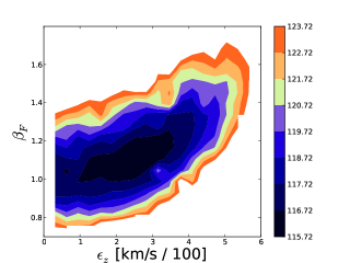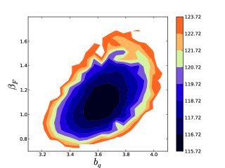
This degeneracy is well illustrated in our model by the $\chi^{2}$ contours for the parameters $\beta_{F}$ and $\epsilon_{z}$, shown in figure 4 (right panel). The quadrupole moment of the cross-correlation is determined mostly by these two parameters. The quadrupole moment increases with $\beta_{F}$ and decreases with $\epsilon_{z}$, but the effect of $\epsilon_{z}$ is obviously important only at small radius (the dependence of the quadrupole moment on the quasar bias factor is relatively small because of the requirement $\beta_{q}=f(\Omega)/b_{q}$, which implies a small value for $\beta_{q}$). A modification of our model at small radius owing to the radiation effects of the quasars or non-linearities may modify the best fit values of $\epsilon_{z}$ and $\Delta_{z}$. The left panel of figure 4 also demonstrates that the quasar bias $b_{q}$ tends to slightly increase with increasing $\beta_{F}$ for a given analysis.

The value of $\chi^{2}=116$ for our fiducial model fit for 130 degrees of freedom, and the agreement of the fitted parameters with other independent determinations, shows that the observed cross-correlation is sufficiently well reproduced without the need to include the effect of the quasar ionizing radiation. Clearly, the linear overdensity around the quasar host halo is the dominant effect when measuring the quasar-Ly$\alpha$ cross-correlation away from the line of sight, on large scales and for the luminosities of the BOSS quasars.

The second row of table 1 gives the best fit parameters when all the bins at separations down to $r>7\,h^{-1}\,{\rm Mpc}$ are used. The best fit shifts to a larger redshift distortion parameter of the Ly$\alpha$ forest, a lower quasar bias factor, and a larger quasar redshift error dispersion. The $\chi^{2}$ worsens significantly, with an increase of 48 when adding only 22 degrees of freedom. This result suggests that our 4-parameter model does not include all the important physical effects when analyzing the entire range of separations in figure 2. Non-linearities and radiation effects are likely to play a role at small separations, and a more complex analysis will be required to discern this.

4.2 Bootstrap errors

In general, we have tested that the bootstrap errors computed as described in section 3 are in agreement with the errors derived from the covariance matrix. We mention here as an example this error comparison for the quasar bias factor, when keeping the other parameters fixed to their best fit value of our fiducial analysis. The covariance matrix yields errors from the $\Delta\chi^{2}=1$ contour of $b_{q}=3.634^{+0.138}_{-0.138}$, and the result of 100 bootstrap realizations from the 12 subsamples of our data set (see [49]) is $b_{q}=3.657\pm 0.135$, in perfect agreement with the standard analysis. In the rest of the paper we use the uncertainties set by the contours of $\Delta\chi^{2}=1$.

4.3 Scale dependence of the quasar bias factor

Figure 5: Fitted QSO bias $b_{q}$ in several bins of the separation $r$, when fixing the other parameters to their best fit value in the fiducial model, $\beta_{F}=1.1$, $\epsilon_{z}=2.42\,h^{-1}\,{\rm Mpc}$, $\Delta_{z}=-1.57\,h^{-1}\,{\rm Mpc}$. The horizontal lines show the best fit and uncertainties when using all separations larger than $r>15\,h^{-1}\,{\rm Mpc}$, the scale that is marked with a vertical dotted line in the figure.

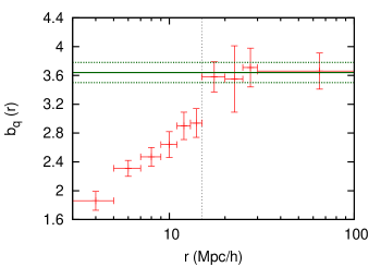
In figure 5 we present the value of the quasar bias that is obtained when using only bins within narrow rings of the separation $r$. For this analysis, we fix the other parameters to their best fit value when using the range $15\,h^{-1}\,{\rm Mpc}<r<100\,h^{-1}\,{\rm Mpc}$, which are $\beta_{F}=1.1$, $\epsilon_{z}=2.42\,h^{-1}\,{\rm Mpc}$, $\Delta_{z}=-1.57\,h^{-1}\,{\rm Mpc}$. The horizontal lines in the figure show the best fit and uncertainties when using all separations above $r>15\,h^{-1}\,{\rm Mpc}$, i.e., all the points lying to the right of the dotted vertical line.

The constancy of the bias factor for $r>15\,h^{-1}\,{\rm Mpc}$ is again a success of the simple linear theory model for large scales, meaning that the radial dependence of the cross-correlation agrees with the prediction of the standard $\Lambda$CDM model of structure formation. The smaller value of $b_{q}$ at smaller separation confirms our previous conclusion that other effects are likely to be important at $r<15\,h^{-1}\,{\rm Mpc}$.

The amplitude of the cross-correlation is proportional to $b_{F}b_{q}\sigma_{8}^{2}$, this is the actual quantity we are measuring, and the value for $b_{q}$ plotted in figure 5 assumes that $b_{F}(1+\beta_{F})=-0.336$ at $z=2.25$ (corrected to the mean quasar redshift $\bar{z}_{q}=2.38$, where $b_{F}(1+\beta_{F})=-0.376$), and $\sigma_{8}=0.8$.

4.4 Impact of the Mean Transmission Correction (MTC)

Our fiducial model uses the Mean Transmission Correction (MTC) as part of the continuum fitting, and corrects the theoretical model accordingly by using the analytical expression derived in appendix A of [49]. As a test of the importance of this correction, table 1 gives the results for two additional models: the NOCOR case (fourth row) treats the observations in the same way as the fiducial model (applying the MTC to the data), but does not correct the theoretical model. The result is a considerably worse fit ($\Delta\chi^{2}=26$), confirming the validity and the need for the theoretical correction. In the NOMTC case, the data for the transmission fluctuation is obtained with the direct use of the PCA continua, without applying the MTC. The uncorrected theory then fits the data properly, but the errors of the best fit parameters are considerably worse, supporting our reasons to use the MTC. An even smaller upper limit for $\epsilon_{z}$ is obtained for the NOMTC case, indicating that this upper limit is questionable because of its degeneracy with other model variations.

Figure 6: Measured cross-correlation in the sixth bin in $\sigma$ ($20\,h^{-1}\,{\rm Mpc}<\sigma<30\,h^{-1}\,{\rm Mpc}$). Red (green) data points correspond to the analysis with (without) the MTC step in the continuum fitting. The black solid (blue dashed) line shows the best fit model for the fiducial analysis with (without) the MTC correction.

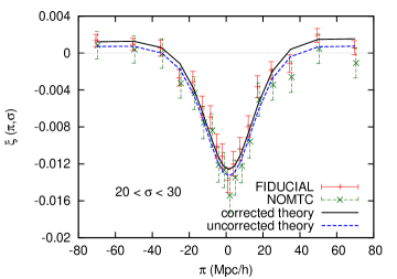
Figure 6 shows the effect of the MTC on the measured cross-correlation, for the sixth bin of $\sigma$ ($20\,h^{-1}\,{\rm Mpc}<\sigma<30\,h^{-1}\,{\rm Mpc}$), as well as the correction we apply to the theoretical model. As seen in the plot, the theoretical correction clearly captures the difference in the analyses. The errorbars in the NOMTC analysis are considerably larger, due to the large spectro-photometric errors present in BOSS quasars. Since these errors have a coherent effect on all pixels of a given spectrum, the errorbars in the NOMTC analysis are strongly correlated.

4.5 Evolution with redshift and variation with quasar luminosity

We test here for the dependence of our measured quasar bias on the redshift and quasar luminosity. In table 1 we show the results obtained when splitting the quasar sample in three redshift bins: LOW-Z (2.00 $<$ z $<$ 2.25), MID-Z (2.25 $<$ z $<$ 2.50) and HIGH-Z (2.50 $<$ z $<$ 3.50). There is no clear evidence of evolution in the quasar bias parameter $b_{q}$, although our errors are large and the redshift range that is probed is limited.

In the same table we show the results obtained when splitting the sample in three luminosity bins: LOW-L for $-25.2<M_{i}<-23.0$, MID-L for $-26.1<M_{i}<-25.2$, and HIGH-L for $-30.0<M_{i}<-26.1$. Again, the changes are not significant, and unfortunately the quasar redshift error distribution may vary with the quasar luminosity, making it difficult to search for any physical dependence of the cross-correlation with quasar luminosity because of the parameter degeneracies.

4.6 Variation with the quasar redshift estimator

There are six different quasar redshift estimators specified in the DR9 quasar catalog ([33]). In the main part of this study we use the PCA redshift estimator (Z_PCA in DR9Q), but we also show in table 1 the results obtained when using the other ones: the visual inspection redshift (Z_VI), the estimator from the BOSS pipeline (Z_PIPELINE), and three estimators that use a single metal absorption line (Z_CII,Z_CIV,Z_MgII).

Table 1 shows the best fit parameters for each of the quasar redshift estimators, and the quasar bias obtained is consistent among them. However, the redshift error distribution varies considerably for the different estimators. Our fits suggest that all the estimators systematically underestimate the quasar redshift by several hundreds of $\,{\rm km\,s}^{-1}$, except for the one based on the MgII line which is basically consistent with $\Delta_{z}=0$, but has a larger dispersion $\epsilon_{z}$.

The presence of a mean redshift displacement can also be tested using narrow emission lines of the quasar host galaxies, namely OII and OIII. The mean redshifts of the MgII and OII lines were compared by [55] in a large sample of low redshift SDSS quasars, who found that the difference had to be smaller than $30\,{\rm km\,s}^{-1}$. This comparison, however, would be difficult to carry out for the higher redshift quasars of our sample, where the OII line is shifted to the infrared.

We caution, however, that these values of $\Delta_{z}$ and $\epsilon_{z}$ are likely to change once our simple four-parameter model is improved with more parameters to include the quasar ionizing radiation effects. The systematic negative value of $\Delta_{z}$ might be adjusting a real asymmetry of the cross-correlation introduced by the reduction of the effective quasar luminosity with the time delay. The effect of the time-delayed quasar ionizing radiation on the cross-correlation should obviously have a different radial dependence than a simple shift of the quasar redshifts, but some degree of degeneracy can be expected. At the same time, it seems difficult to believe that the true dispersion $\epsilon_{z}$, arising from both observational errors and the intrinsic velocity dispersion of quasars within halos, is smaller than $\sim 500\,{\rm km\,s}^{-1}$, and its value will also probably be modified in a more complex model that better reflects the underlying physical effects.

5 Effects of the Quasar Radiation

As we have seen in the previous section, the large-scale form of the quasar-Ly$\alpha$ cross-correlation is consistent with the linear overdensity expected around the quasar host halos. This result may be surprising because of the previous detection of the proximity effect when measuring this cross-correlation along the line of sight, caused by the increased ionization of the intergalactic medium induced by the quasar ionizing radiation, although the BOSS quasars are of lower luminosity than most of the quasars on which the proximity effect was measured and therefore the expected additional ionization is much weaker in our case compared to previous studies. In this section we present a simple estimate of the expected radiation effect on the full three-dimensional cross-correlation with our quasar sample. A more detailed analysis involving fitting of a more complex model that includes both the radiation and overdensity effects is left for a future study.

The radiation of a quasar of luminosity $L_{\nu}$ increases the photoionization rate of gas at a proper distance $d$ by the amount

$$\Gamma_{q}={1\over 4\pi d^{2}h}\int_{\nu_{HI}}^{\infty}d\nu\,{L_{\nu}\sigma_{HI}(\nu)\over\nu}~{},$$ (5.1)

where $\nu_{HI}$ is the hydrogen Lyman limit frequency, $\sigma_{HI}$ is the photoionization cross section, and $h$ is the Planck constant. We neglect here the absorption by Lyman limit systems and the redshifting of the radiation, which reduces the quasar intensity when $d$ is comparable to the absorption mean free path or the local horizon. Let the relative fluctuation of the photoionization rate relative to its average value $\Gamma_{0}$ be $\delta_{\Gamma}$. In general, $\delta_{\Gamma}$ can be affected by many sources. Neglecting the effects of ionizing source clustering (which increases the mean ionizing flux near a quasar beyond that emitted by the quasar itself), assuming a quasar spectrum $L_{\nu}\propto\nu^{-\alpha}$, and approximating $\sigma_{HI}(\nu)\propto\nu^{-3}$ at $\nu>\nu_{HI}$, the average value of $\delta_{\Gamma}$ near the quasar is

$$\delta_{\Gamma}={\Gamma_{q}\over\Gamma_{0}}\simeq{L_{\nu_{HI}}\sigma_{HI}(\nu_{HI})\over 4\pi d^{2}h\Gamma_{0}(3+\alpha)}~{}.$$ (5.2)

The impact of the perturbation $\delta_{\Gamma}$ on the Ly$\alpha$ forest can be calculated using the approximation that the gas is purely photoionized (neglecting any contribution from collisional ionization) and that the neutral fraction is everywhere much smaller than unity. In this case, the optical depth at any point in the spectrum of the Ly$\alpha$ forest is inversely proportional to the photoionization rate, so the fractional perturbation in the optical depth is $\delta_{\tau}=1/(1+\delta_{\Gamma})-1\simeq-\delta_{\Gamma}$, where the last approximate equality assumes $\delta_{\Gamma}\ll 1$. Now, let $F_{0}=e^{-\tau_{0}}$ be the Ly$\alpha$ transmission fraction when the photoionization rate has the uniform value $\Gamma_{0}$, with a distribution $P(F_{0})$. The transmission in the presence of radiation fluctuations is $F=e^{-\tau_{0}(1-\delta_{\Gamma})}$, and the mean transmission is

$$\bar{F} =\int_{0}^{1}dF_{0}\,P(F_{0})\,e^{-\tau_{0}(1-\delta_{\Gamma})}$$ (5.3)

$$\simeq\int_{0}^{1}dF_{0}\,P(F_{0})\,F_{0}(1+\tau_{0}\delta_{\Gamma})$$

$$\simeq\bar{F}_{0}-\delta_{\Gamma}\int_{0}^{1}dF_{0}\,P(F_{0})\,F_{0}\,\log(F_{0})~{}.$$

We can now define the radiation bias factor of the Ly$\alpha$ forest, $b_{\Gamma}$, as the linear variation of the mean transmission fluctuation $\delta_{F}$ in response to a fractional variation $\delta_{\Gamma}$ in the radiation intensity, analogously to the density and peculiar velocity gradient bias factors. Hence, near a quasar the mean transmission fluctuation will vary by $\delta_{F}=b_{\Gamma}\delta_{\Gamma}$ owing to the fractional radiation perturbation $\delta_{\Gamma}$, where

$$b_{\Gamma}=-\frac{1}{\bar{F}}\int_{0}^{1}dF_{0}\,P(F_{0})\,F_{0}\,\ln(F_{0})~{}.$$ (5.4)

If we use as the transmission distribution a log-normal function in the optical depth, with mean $\bar{F}_{0}=0.8$ and dispersion $\sigma_{F}=0.124$, which is close to the observed distribution at $z=2.3$, we find $b_{\Gamma}=0.13$.

We now estimate the average intensity produced by the quasars in our sample. The mean flux per unit frequency of a quasar of magnitude $g$ is $f_{\nu}=10^{-0.4(48.6+g)}$, expressed in cgs units ([40]). The mean value of $f_{\nu}$ we obtain for our quasar sample is $f_{\nu}=2.4\times 10^{-28}\,{\rm erg}\,{\rm s}^{-1}{\rm cm}^{-2}\,{\rm Hz}^{-1}$ at the center of the $g$-band (at $4800\,{\rm\AA}$; this corresponds to a $g$ magnitude of 20.5) At the mean redshift $\bar{z}_{q}=2.38$ of our quasar sample, the implied mean luminosity at the shifted $g$-band center $\lambda=1420\,{\rm\AA}$ is $L_{\nu}=4\pi D_{L}^{2}f_{\nu}/(1+\bar{z}_{q})=3.1\times 10^{30}\,{\rm erg}\,{\rm s}^{-1}\,{\rm Hz}^{-1}$. We assume a mean spectral slope from this wavelength to the Lyman limit wavelength $L_{\nu}\propto\nu^{-1}$ ([56], [57]) , which results in $L_{\nu_{HI}}=2.0\times 10^{30}\,{\rm erg}\,{\rm s}^{-1}\,{\rm Hz}^{-1}$. The corresponding quasar flux at a characteristic comoving distance of interest of $d(1+\bar{z}_{q})=20\,h^{-1}\,{\rm Mpc}$, or proper distance $d=8.33\,{\rm Mpc}$, is then $f_{\nu_{HI}}=2.4\times 10^{-22}\,{\rm erg}\,{\rm s}^{-1}{\rm cm}^{-2}\,{\rm Hz}^{-1}$. Finally, using equation (5.2) with the spectral index $\alpha=1.5$ for $\nu>\nu_{HI}$, the derived photoionization rate is $\Gamma_{q}=5.1\times 10^{-14}\,{\rm s}^{-1}$.

If we assume a mean photoionization rate from the average of all sources $\Gamma_{0}=10^{-12}\,{\rm s}^{-1}$, then at this comoving distance of $20\,h^{-1}\,{\rm Mpc}$, we have $\delta_{\Gamma}\simeq 0.05$, and the mean perturbation on the transmission should be $\delta_{F}\simeq b_{\Gamma}\delta_{\Gamma}\simeq 0.0065$. In the absence of any absorption effects, this perturbation should vary in proportion to $d^{-2}$.

Comparing to figure 3, we see that this radiation effect should displace the value of the cross-correlation by one contour at $r=(\sigma^{2}+\pi^{2})^{1/2}=20\,h^{-1}\,{\rm Mpc}$. In the third panel of figure 2 (for the range $7\,h^{-1}\,{\rm Mpc}<\sigma<10\,h^{-1}\,{\rm Mpc}$), the increase of the cross-correlation would be $\sim 0.03$ at small $\pi$, which is larger than the difference between the data points and our fiducial model fit, and in the fifth panel (for the range $15\,h^{-1}\,{\rm Mpc}<\sigma<20\,h^{-1}\,{\rm Mpc}$), the increase would be $\sim 0.008$. These changes would significantly affect our fiducial fit, implying a substantial increase of $b_{q}$ in order to compensate for the radiation effect to a value $b_{q}\simeq 5$, which would disagree with the autocorrelation measurement of [12]. We therefore suspect that the quasar radiation effect is reduced relative to this simple estimate.

The effect of the ionizing radiation is not expected to be isotropic around the quasar in redshift space. Quasars are likely to emit their light anisotropically, with lower intensity near the plane of the accretion disk around the black hole. A flux limited sample of quasars preferentially selects sources with their axis (the direction of brightest emission) near our line of sight, so on average the flux from quasars in the perpendicular direction should be lower than in the parallel direction. Time variability of the quasars also implies that the mean quasar ionizing flux affecting the Ly$\alpha$ forest depends on the time delay, $ct_{d}=r+\pi$: the Ly$\alpha$ forest is illuminated by the luminosity of the quasar at a time $t_{d}$ before the epoch when we are observing. The selection effect again causes the average quasar in a flux-limited sample to have lower luminosity in the past compared to the present, and this should introduce an asymmetry depending on the sign of $\pi$. A hint of this signature of the radiation effect is seen in figure 2, in the region $\pi\simeq-20\,h^{-1}\,{\rm Mpc}$ and $\sigma<|\pi|$, which is consistent with the increase of $\delta_{F}\simeq 0.007$ we have estimated at $r=20\,h^{-1}\,{\rm Mpc}$ from the radiation effect. If this hint is correct, quasars might shine at close to the expected luminosities within $\sim 45^{\circ}$ of the line of sight and for time delays $t_{d}<10^{7}$ years, and have effective lower luminosities at larger angles from the line of sight and for longer time delays.

In any case, obtaining solid conclusions on the contribution of the radiation effect to the cross-correlation and the statistical significance of any detection requires a more detailed modeling with more fitting parameters, additional data and a more careful inclusion of all the important effects. We plan to perform this study in the future when the BOSS survey is completed. We mention here, however, that the radiation effects we have discussed may be altering the value of the linear model parameters we have fitted. In particular, the redshift offset $\Delta_{z}$ may in part be the result of the attempt to adjust the radiation and time-delay effect which introduces the asymmetry depending on the sign of $\pi$.

Non-linear effects in the clustering of both quasars and Ly$\alpha$ absorption, as well as the non-linearity in the relation between optical depth and transmitted flux fraction, may also have an impact on the cross-correlation at small scales. However, we compared the linear theory predictions to the results of numerical simulations of [30] for the cross-correlation, and we found that non-linearities become important only at scales smaller than a few $\,h^{-1}\,{\rm Mpc}$, whereas the radiation effects are a more important correction at intermediate scales of $\sim 10\,h^{-1}\,{\rm Mpc}$.

Finally, we note that HeII reionization may alter the IGM temperature near quasars because of the additional heating involved ([58], [59]), which may result in an additional effect on the cross-correlation. The effect would likely also vary as the inverse squared distance from the quasar. However, the duration of the HeII reionization is probably much longer than the typical lifetime of a quasar, implying that most of the temperature fluctuations originated from the HeII reionization would be caused by quasars that have long been dead.

5.1 Predictions for the proximity effect

Our fitted linear theory model for the mean overdensity around a quasar can be used to make a prediction on the impact of this overdensity on any measurements of the proximity effect of quasars on the line of sight due to their ionizing radiation. In figure 7, we show the prediction for the line of sight cross-correlation, as $\pi\xi(\sigma=0,\pi)$, for our two first models in table 1: 1) the fiducial model fit using pixels at $r>15\,h^{-1}\,{\rm Mpc}$ (solid, black line), and 2) the same model using all pixels at $r>7\,h^{-1}\,{\rm Mpc}$ (dashed, blue line; in this subsection we choose the convention that $\pi$ is positive even though for the three-dimensional discussion $\pi$ is negative in front of the quasar). Also shown as the red, dotted line is the expected radiation effect in our sample of quasars, which we have plotted according to our simple estimate above as $\xi=0.0065(20\,h^{-1}\,{\rm Mpc}/\pi)^{2}$. Note that this curve is proportional to the mean quasar luminosity, so the proximity effect due to the radiation dominates over the overdensity effect for quasars of much greater luminosity than the ones in the BOSS sample.

Figure 7: Cross-correlation function along the line of sight, i.e., using pixels and their background quasar. The black solid (blue dashed) line shows our best fit theory for $r>15\,h^{-1}\,{\rm Mpc}$ ($r>7\,h^{-1}\,{\rm Mpc}$). The dotted red line shows the expected radiation effect.

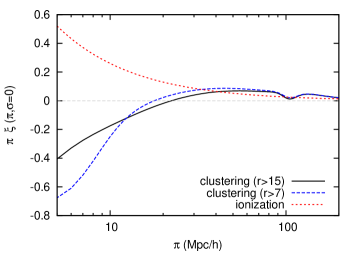
As shown in this figure, the overdensity effect should roughly cancel the radiation effect at $\pi\sim 10\,h^{-1}\,{\rm Mpc}$ for the luminosities of typical BOSS quasars. Most studies of the proximity effect have used brighter quasars to obtain higher signal-to-noise spectra, but figure 7 provides a correction that should be applied to any future measurements of the proximity effect due to radiation under the assumption that the quasar bias factor does not depend on quasar luminosity. For $\pi>20\,h^{-1}\,{\rm Mpc}$, the overdensity effect causes an increased $\delta_{F}$ (decreased absorption) that is therefore added to any radiation effect, because the peculiar velocity gradient due to the infall of matter toward the quasar halo is a more important effect than the overdensity.

6 Conclusions

We have measured the cross-correlation of quasars and the Ly$\alpha$ forest transmission in redshift space using more than 60000 quasars from BOSS. This unprecedentedly large number of quasar spectra for such a study has allowed a statistically significant detection of this cross-correlation out to separations of $\sim 80\,h^{-1}\,{\rm Mpc}$, and a detailed determination of its radial and angular dependence. The cross-correlation is consistent with the linear theory prediction of the standard $\,\rm\Lambda$CDM model, with the expected redshift distortions, on scales $r>15\,h^{-1}\,{\rm Mpc}$. Fitting these large-scale measurements to a linear model with four parameters, we find that the BOSS quasars at $\bar{z}_{q}=2.38$ have a mean bias factor $b_{q}=3.64^{+0.13}_{-0.15}$. This result is consistent with the quasar bias measured from the auto-correlation of a sub-sample of the same quasars, $b_{q}=3.8\pm 0.3$, as presented in [12]. The halo mass having this bias factor is $M_{h}\simeq 3\times 10^{12}\ h^{-1}M_{\odot}$. This measurement can be compared to the halo mass corresponding to the mean bias factor inferred for DLAs, the other population of objects for which the bias factor was measured from the same approach measuring the cross-correlation with the Ly$\alpha$ forest in BOSS, which was $M_{h}\simeq 4\times 10^{11}\ h^{-1}M_{\odot}$, although a large scatter in halo masses is expected for both populations of objects and only the mean bias factor is measured. We do not detect any dependence of quasar bias on luminosity or redshift, also consistent with the results from [12].

The large-scale fit to the cross-correlation also provides a measurement of the Ly$\alpha$ forest redshift distortion parameter, $\beta_{F}=1.1^{+0.17}_{-0.15}$. This value is $\sim 1.5\sigma$ higher than the one measured in [4], reducing the tension with previous numerical simulations ([60]). The value of $\beta_{F}$ measured from this cross-correlation has the advantage of being less sensitive to systematic errors in the spectrophotometric calibration, although it should be equally affected by the presence of DLAs, Lyman limit systems and metal lines in the spectra which tend to decrease $\beta_{F}$ ([61]).

The cross-correlation at scales $r<15\,h^{-1}\,{\rm Mpc}$ is not well fitted by the simple linear theory model we have used, because its amplitude is lower than expected in the model fitted to large scales, as seen in figure 5. We have argued that a likely explanation is the effects of the ionizing radiation of the quasars, which are of the right order of magnitude to explain this discrepancy for the luminosity of the BOSS quasars. If all the BOSS quasars emitted their light isotropically and with constant luminosities, the enhanced ionization of the surrounding medium would also affect the cross-correlation we have fitted at $r>15\,h^{-1}\,{\rm Mpc}$, implying a higher quasar bias factor to compensate for this ionization effect. However, the quasar radiation effect is likely to be decreased owing to anisotropic emission and finite quasar lifetimes.

The impact of the quasar ionization can also be studied by means of the line of sight proximity effect, and using the cross-correlation measured from especially targeted quasar pairs at smaller angular separations than in the BOSS sample. In the future, these studies will need to model the superposed effects of the mean overdensity around the quasar host halos and the ionization effects. Here, we have presented predictions from our fitted models for the correction that needs to be applied to the line of sight proximity effect for the mean overdensity around quasars, before attempting to infer anything about the ionization effect of the quasar. This correction has been neglected in the past ([17], [18],[19], [20]), and is in fact small for the most luminous quasars that have been used to study the proximity effect, but becomes important for quasars of luminosities typical of the BOSS sample.

The expected redshift distortions also imply that the effect of the overdensity is smaller on the line of sight compared to the perpendicular direction, and changes sign at separations $|\pi|\gtrsim 20\,h^{-1}\,{\rm Mpc}$ owing to the induced peculiar velocity gradient. We note that this predicted correction assumes linear theory, so it can be altered at small scales.

The quasar-Ly$\alpha$ cross-correlation can also be useful to constrain the redshift errors of the quasars. Our results for the mean redshift offset $\Delta z$ indicate that the quasar estimators that have been used are systematically too low, except for the one based on MgII which is closest to zero. We have warned, however, that the result for this redshift offset may be affected by the quasar radiation effect with finite quasar lifetimes, which can introduce an asymmetry depending on the sign of $\pi$.

Future studies of the quasar-Ly$\alpha$ cross-correlation have a promising potential for probing both the large-scale distribution of matter around quasars and the characteristics of the ionizing emission. The Baryon Acoustic Oscillation peak, detected recently in the Ly$\alpha$ autocorrelation ([54],[62]), can also be detected in the quasar-Ly$\alpha$ cross-correlation. The ratio of the BAO peak amplitudes in the monopole, $\xi^{BAO}_{q\alpha}/\xi^{BAO}_{\alpha\alpha}$, should be equal to ([35])

$${\xi^{BAO}_{q\alpha}\over\xi^{BAO}_{\alpha\alpha}}={b_{q}\over b_{F}}\,{1+(\beta_{F}+\beta_{q})/3+\beta_{F}\beta_{q}/5\over 1+2\beta_{F}/3+\beta_{F}^{2}/5}~{}.$$ (6.1)

Using the values $b_{q}=3.7$, $\beta_{F}=1.1$, and $b_{F}=0.16$, we find $\xi^{BAO}_{q\alpha}/\xi^{BAO}_{\alpha\alpha}\simeq 18$, and using $\xi^{BAO}_{\alpha\alpha}\simeq 2\times 10^{-5}$ ([54]), we expect $\xi^{BAO}_{q\alpha}\simeq 4\times 10^{-4}$. This BAO peak should be detectable in the cross-correlation before the end of the BOSS survey (see figure 2). At the same time, detailed modeling of the cross-correlation on a broad range of scales will hopefully allow for the separation of the overdensity and radiation effects, allowing for a measurement of the characteristic anisotropy of quasar emission and of the lifetimes of quasars.

References

- [1] R. Lynds, Astrophys. J. Let. 164, L73+ (Mar. 1971).
- [2] M. Rauch, ARAA 36, 267 (1998), arXiv:astro-ph/9806286.
- [3] P. McDonald, U. Seljak, S. Burles, D. J. Schlegel, D. H. Weinberg, R. Cen, D. Shih, J. Schaye, D. P. Schneider, N. A. Bahcall, et al., Astrophys. J. Sup. 163, 80 (Mar. 2006), arXiv:astro-ph/0405013.
- [4] A. Slosar, A. Font-Ribera, M. M. Pieri, J. Rich, J.-M. Le Goff, É. Aubourg, J. Brinkmann, N. Busca, B. Carithers, R. Charlassier, et al., JCAP 9, 1 (Sep. 2011), 1104.5244.
- [5] C. Porciani, M. Magliocchetti, and P. Norberg, Mon. Not. Roy. Astron. Soc. 355, 1010 (Dec. 2004), astro-ph/0406036.
- [6] S. M. Croom, B. J. Boyle, T. Shanks, R. J. Smith, L. Miller, P. J. Outram, N. S. Loaring, F. Hoyle, and J. da Ângela, Mon. Not. Roy. Astron. Soc. 356, 415 (Jan. 2005), arXiv:astro-ph/0409314.
- [7] J. da Ângela, P. J. Outram, T. Shanks, B. J. Boyle, S. M. Croom, N. S. Loaring, L. Miller, and R. J. Smith, Mon. Not. Roy. Astron. Soc. 360, 1040 (Jul. 2005), arXiv:astro-ph/0504438.
- [8] A. D. Myers, R. J. Brunner, G. T. Richards, R. C. Nichol, D. P. Schneider, D. E. Vanden Berk, R. Scranton, A. G. Gray, and J. Brinkmann, Astrophys. J. 638, 622 (Feb. 2006), arXiv:astro-ph/0510371.
- [9] Y. Shen, M. A. Strauss, M. Oguri, J. F. Hennawi, X. Fan, G. T. Richards, P. B. Hall, J. E. Gunn, D. P. Schneider, A. S. Szalay, et al., AJ 133, 2222 (May 2007), arXiv:astro-ph/0702214.
- [10] N. P. Ross, Y. Shen, M. A. Strauss, D. E. Vanden Berk, A. J. Connolly, G. T. Richards, D. P. Schneider, D. H. Weinberg, P. B. Hall, N. A. Bahcall, et al., Astrophys. J. 697, 1634 (Jun. 2009), 0903.3230.
- [11] Y. Shen, M. A. Strauss, N. P. Ross, P. B. Hall, Y.-T. Lin, G. T. Richards, D. P. Schneider, D. H. Weinberg, A. J. Connolly, X. Fan, et al., Astrophys. J. 697, 1656 (Jun. 2009), 0810.4144.
- [12] M. White, A. D. Myers, N. P. Ross, D. J. Schlegel, J. F. Hennawi, Y. Shen, I. McGreer, M. A. Strauss, A. S. Bolton, J. Bovy, et al., Mon. Not. Roy. Astron. Soc. 424, 933 (Aug. 2012), 1203.5306.
- [13] K. L. Adelberger and C. C. Steidel, Astrophys. J. Let. 627, L1 (Jul. 2005), arXiv:astro-ph/0505546.
- [14] A. L. Coil, J. F. Hennawi, J. A. Newman, M. C. Cooper, and M. Davis, Astrophys. J. 654, 115 (Jan. 2007).
- [15] N. Padmanabhan, M. White, P. Norberg, and C. Porciani, Mon. Not. Roy. Astron. Soc. 397, 1862 (Aug. 2009), 0802.2105.
- [16] Vikas++, QSO - CIV cross-correlation (should be done in a couple of weeks, update), , in preparation (2013).
- [17] R. F. Carswell, J. A. J. Whelan, M. G. Smith, A. Boksenberg, and D. Tytler, Mon. Not. Roy. Astron. Soc. 198, 91 (Jan. 1982).
- [18] H. S. Murdoch, R. W. Hunstead, M. Pettini, and J. C. Blades, Astrophys. J. 309, 19 (Oct. 1986).
- [19] S. Bajtlik, R. C. Duncan, and J. P. Ostriker, Astrophys. J. 327, 570 (Apr. 1988).
- [20] J. Scott, J. Bechtold, A. Dobrzycki, and V. P. Kulkarni, Astrophys. J. Sup. 130, 67 (Sep. 2000), arXiv:astro-ph/0004155.
- [21] P. Jakobsen, M. A. C. Perryman, S. di Serego Alighieri, M. H. Ulrich, and F. Macchetto, Astrophys. J. Let. 303, L27 (Apr. 1986).
- [22] A. P. S. Crotts, Astrophys. J. 336, 550 (Jan. 1989).
- [23] P. Moller and P. Kjaergaard, A&A 258, 234 (May 1992).
- [24] J. Liske and G. M. Williger, Mon. Not. Roy. Astron. Soc. 328, 653 (Dec. 2001), arXiv:astro-ph/0108239.
- [25] D. J. Schlegel, D. P. Finkbeiner, and M. Davis, Astrophys. J. 500, 525 (Jun. 1998).
- [26] M. Schirber, J. Miralda-Escudé, and P. McDonald, Astrophys. J. 610, 105 (Jul. 2004), arXiv:astro-ph/0307563.
- [27] R. A. C. Croft, Astrophys. J. 610, 642 (Aug. 2004), arXiv:astro-ph/0310890.
- [28] E. Rollinde, R. Srianand, T. Theuns, P. Petitjean, and H. Chand, Mon. Not. Roy. Astron. Soc. 361, 1015 (Aug. 2005), arXiv:astro-ph/0502284.
- [29] R. Guimarães, P. Petitjean, E. Rollinde, R. R. de Carvalho, S. G. Djorgovski, R. Srianand, A. Aghaee, and S. Castro, Mon. Not. Roy. Astron. Soc. 377, 657 (May 2007), arXiv:astro-ph/0702369.
- [30] Y.-R. Kim and R. A. C. Croft, Mon. Not. Roy. Astron. Soc. 387, 377 (Jun. 2008).
- [31] D. J. Eisenstein, D. H. Weinberg, E. Agol, H. Aihara, C. Allende Prieto, S. F. Anderson, J. A. Arns, É. Aubourg, S. Bailey, E. Balbinot, et al., AJ 142, 72 (Sep. 2011), 1101.1529.
- [32] K. S. Dawson, D. J. Schlegel, C. P. Ahn, S. F. Anderson, É. Aubourg, S. Bailey, R. H. Barkhouser, J. E. Bautista, A. Beifiori, A. A. Berlind, et al., AJ 145, 10, 10 (Jan. 2013), 1208.0022.
- [33] I. Pâris, P. Petitjean, É. Aubourg, S. Bailey, N. P. Ross, A. D. Myers, M. A. Strauss, S. F. Anderson, E. Arnau, J. Bautista, et al., A&A 548, A66, A66 (Dec. 2012), 1210.5166.
- [34] N. Kaiser, Mon. Not. Roy. Astron. Soc. 227, 1 (Jul. 1987).
- [35] A. J. S. Hamilton, Astrophys. J. Let. 385, L5 (Jan. 1992).
- [36] E. Komatsu, K. M. Smith, J. Dunkley, C. L. Bennett, B. Gold, G. Hinshaw, N. Jarosik, D. Larson, M. R. Nolta, L. Page, et al., Astrophys. J. Sup. 192, 18, 18 (Feb. 2011), 1001.4538.
- [37] C. P. Ahn, R. Alexandroff, C. Allende Prieto, S. F. Anderson, T. Anderton, B. H. Andrews, É. Aubourg, S. Bailey, E. Balbinot, R. Barnes, et al., Astrophys. J. Sup. 203, 21, 21 (Dec. 2012), 1207.7137.
- [38] A. S. Bolton, D. J. Schlegel, É. Aubourg, S. Bailey, V. Bhardwaj, J. R. Brownstein, S. Burles, Y.-M. Chen, K. Dawson, D. J. Eisenstein, et al., AJ 144, 144, 144 (Nov. 2012), 1207.7326.
- [39] J. E. Gunn, M. Carr, C. Rockosi, M. Sekiguchi, K. Berry, B. Elms, E. de Haas, Ž. Ivezić, G. Knapp, R. Lupton, et al., AJ 116, 3040 (Dec. 1998).
- [40] M. Fukugita, T. Ichikawa, J. E. Gunn, M. Doi, K. Shimasaku, and D. P. Schneider, AJ 111, 1748 (Apr. 1996).
- [41] J. E. Gunn, W. A. Siegmund, E. J. Mannery, R. E. Owen, C. L. Hull, R. F. Leger, L. N. Carey, G. R. Knapp, D. G. York, W. N. Boroski, et al., AJ 131, 2332 (Apr. 2006), arXiv:astro-ph/0602326.
- [42] S. Smee, J. E. Gunn, A. Uomoto, N. Roe, D. Schlegel, C. M. Rockosi, M. A. Carr, F. Leger, K. S. Dawson, M. D. Olmstead, et al., ArXiv e-prints (Aug. 2012), 1208.2233.
- [43] D. G. York, J. Adelman, J. E. Anderson, S. F. Anderson, J. Annis, N. A. Bahcall, J. A. Bakken, R. Barkhouser, S. Bastian, E. Berman, et al., AJ 120, 1579 (Sep. 2000).
- [44] K.-G. Lee, S. Bailey, L. E. Bartsch, W. Carithers, K. S. Dawson, D. Kirkby, B. Lundgren, D. Margala, N. Palanque-Delabrouille, M. M. Pieri, et al., AJ 145, 69, 69 (Mar. 2013), 1211.5146.
- [45] N. P. Ross, A. D. Myers, E. S. Sheldon, C. Yèche, M. A. Strauss, J. Bovy, J. A. Kirkpatrick, G. T. Richards, É. Aubourg, M. R. Blanton, et al., Astrophys. J. Sup. 199, 3, 3 (Mar. 2012), 1105.0606.
- [46] C. Yèche, P. Petitjean, J. Rich, E. Aubourg, N. Busca, J.-C. Hamilton, J.-M. Le Goff, I. Paris, S. Peirani, C. Pichon, et al., A&A 523, A14, A14 (Nov. 2010).
- [47] J. A. Kirkpatrick, D. J. Schlegel, N. P. Ross, A. D. Myers, J. F. Hennawi, E. S. Sheldon, D. P. Schneider, and B. A. Weaver, Astrophys. J. 743, 125, 125 (Dec. 2011), 1104.4995.
- [48] J. Bovy, J. F. Hennawi, D. W. Hogg, A. D. Myers, J. A. Kirkpatrick, D. J. Schlegel, N. P. Ross, E. S. Sheldon, I. D. McGreer, D. P. Schneider, et al., Astrophys. J. 729, 141, 141 (Mar. 2011), 1011.6392.
- [49] A. Font-Ribera, J. Miralda-Escudé, E. Arnau, B. Carithers, K.-G. Lee, P. Noterdaeme, I. Pâris, P. Petitjean, J. Rich, E. Rollinde, et al., JCAP 11, 59, 059 (Nov. 2012), 1209.4596.
- [50] P. Noterdaeme, P. Petitjean, W. C. Carithers, I. Pâris, A. Font-Ribera, S. Bailey, E. Aubourg, D. Bizyaev, G. Ebelke, H. Finley, et al., A&A 547, L1, L1 (Nov. 2012), 1210.1213.
- [51] Carithers++, Concordance DLA Catalogue, , in preparation (2013).
- [52] K.-G. Lee, N. Suzuki, and D. N. Spergel, AJ 143, 51, 51 (Feb. 2012).
- [53] C.-A. Faucher-Giguère, J. X. Prochaska, A. Lidz, L. Hernquist, and M. Zaldarriaga, Astrophys. J. 681, 831 (Jul. 2008), 0709.2382.
- [54] N. G. Busca, T. Delubac, J. Rich, S. Bailey, A. Font-Ribera, D. Kirkby, J.-M. Le Goff, M. M. Pieri, A. Slosar, É. Aubourg, et al., A&A 552, A96, A96 (Apr. 2013), 1211.2616.
- [55] P. C. Hewett and V. Wild, Mon. Not. Roy. Astron. Soc. 405, 2302 (Jul. 2010), 1003.3017.
- [56] D. E. Vanden Berk, G. T. Richards, A. Bauer, M. A. Strauss, D. P. Schneider, T. M. Heckman, D. G. York, P. B. Hall, X. Fan, G. R. Knapp, et al., AJ 122, 549 (Aug. 2001), arXiv:astro-ph/0105231.
- [57] J. M. Shull, M. Stevans, and C. W. Danforth, Astrophys. J. 752, 162, 162 (Jun. 2012), 1204.3908.
- [58] J. Miralda-Escudé and M. J. Rees, Mon. Not. Roy. Astron. Soc. 266, 343 (Jan. 1994).
- [59] M. McQuinn, A. Lidz, M. Zaldarriaga, L. Hernquist, P. F. Hopkins, S. Dutta, and C.-A. Faucher-Giguère, Astrophys. J. 694, 842 (Apr. 2009), 0807.2799.
- [60] P. McDonald, Astrophys. J. 585, 34 (Mar. 2003), arXiv:astro-ph/0108064.
- [61] A. Font-Ribera and J. Miralda-Escudé, JCAP 7, 28 (Jul. 2012), 1205.2018.
- [62] A. Slosar, V. Iršič, D. Kirkby, S. Bailey, N. G. Busca, T. Delubac, J. Rich, É. Aubourg, J. E. Bautista, V. Bhardwaj, et al., JCAP 4, 26, 026 (Apr. 2013), 1301.3459.